Marine Voyage Optimization and Weather Routing with Deep Reinforcement Learning

Abstract

Marine voyage optimization determines the optimal route and speed to ensure timely arrival. The problem becomes particularly complex when incorporating a dynamic environment, such as future expected weather conditions along the route and unexpected disruptions. This study explores two model-free Deep Reinforcement Learning (DRL) algorithms: (i) a Double Deep Q Network (DDQN) and (ii) a Deep Deterministic Policy Gradient (DDPG). These algorithms are computationally costly, so we split optimization into an offline phase (costly pre-training for a route) and an online phase where the algorithms are fine-tuned as updated weather data become available. Fine tuning is quick enough for en-route adjustments and for updating the offline planning for different dates where the weather might be very different. The models are compared to classical and heuristic methods: the DDPG achieved a 4% lower fuel consumption than the DDQN and was only outperformed by Tabu Search by 1%. Both DRL models demonstrate high adaptability to dynamic weather updates, achieving up to 12% improvement in fuel consumption compared to the distance-based baseline model. Additionally, they are non-graph-based and self-learning, making them more straightforward to extend and integrate into future digital twin-driven autonomous solutions, compared to traditional approaches.

1. Introduction

International trade has expanded significantly with the rapid economic globalization of the past decades. In this, maritime transport has been pivotal, carrying around 80% of goods by value [1]. Ships have played a crucial role in supporting trade due to their energy efficiency, large cargo capacity, and, therefore, high-cost effectiveness [1,2]. However, the rising demand for maritime transport brings new challenges in operational efficiency, cost management, and environmental impact.

Today it is clear that human activity is accelerating climate change [3] and several global economy sectors, including maritime shipping, face mounting pressure to reduce their carbon footprint [4]. The International Maritime Organization (IMO) adopted its initial decarbonization strategy in 2018, later revising it in 2023 with the ambition of achieving net-zero greenhouse gas (GHG) emissions by mid-century and partially adopting near zero GHG technologies by 2030 [5,6]. In parallel, the European Union has integrated shipping emission into its Emissions Trading System (EU-ETS) from 2024 onward, marking a significant regulatory shift to curb emissions from the sector [7].

In response to these challenges, voyage optimization has emerged as a promising solution to enhance route planning by integrating real-time information, vessel performance models, and data-driven decision making. Fuel costs are a major component of a carrier’s operational expenses; thus, even minor route improvements yield substantial financial and environmental benefits [8]. Voyage optimization involves selecting the optimal route while considering several factors such as weather conditions (e.g., wind, waves, currents, and sea state), fuel consumption, departure and arrival windows, as well as safety and regulatory compliance. Studies on the European fleet indicate that reducing sailing speed alone could yield emission reductions of 4–27%, while combining technical and operational measures might achieve an additional 3–28% reduction [9]. The impact of speed optimization on emissions varies, with potential savings ranging from a median of 20% to as high as 80%, depending on route characteristics, vessel type, and meteorological conditions [10].

Traditional weather routing primarily focuses on avoiding adverse weather to ensure safety and minimize travel time, often leading to estimated emissions savings of 10% or less. However, these savings can be improved when weather routing is integrated with other operational measures, such as environmental routing, which explicitly incorporates emission reduction into decision making [11]. Risk assessment is also vital, as operators must evaluate the probability of encountering extreme weather events, the financial risks associated with Just-in-Time (JIT) arrivals and the potential penalties for delays or increased fuel consumption [12].

The research gap arises from the limitations of current weather routing models, which often fail to integrate real-time data effectively. Our work leverages cutting-edge optimization techniques and real-time data integration to propose a novel approach for minimizing fuel consumption for a typical container ship traveling from port A to port B. The proposed adaptive routing methodology responds dynamically to evolving environmental conditions, offering a level of flexibility and responsiveness that is often absent in current methodologies. The strategy aims to maintain a specified estimated time of arrival (ETA) window while minimizing total fuel consumption, directly correlating to reduced CO₂ emissions. The work has been carried out within the activities of the HEU DT4GS project, which builds digital twins for shipping, ensuring integration with digital twin systems through the necessary data streams.

We contribute to the literature by presenting two distinct model-free Deep Reinforcement Learning (DRL) techniques, the Deep Double Q-Network (DDQN) and Deep Deterministic Policy Gradient (DDPG). Our contribution lies in analyzing these two DRL approaches and evaluating how their distinct action space characteristics influence performance in optimizing fuel consumption. The DDQN operates in a discrete action space suitable for problems with a predefined set of actions, while the DDPG enables fine-grained control through its continuous action space, making it particularly well suited for real-world maritime navigation scenarios.

A novel aspect of this work is the consideration of complex routes with obstacles and confined waterways. To address this challenge, we implement the ‘teleportation’ concept, allowing the optimization to pause and restart and the vessel to navigate through tight, congested areas by seamlessly transitioning between entry and exit points. This method introduces a new layer of route flexibility, improving upon previous approaches that tend to optimize less complex, oceanic tracks.

We also benchmark the performance of the DRL models against classical and heuristic algorithms, proving a comprehensive assessment of their relative performance, strengths, and limitations. We find that both DRL techniques perform well in terms of fuel consumption reduction, with the DDPG only slightly outperformed by Tabu Search. At the same time, the DRL solutions demonstrate strong adaptability in dynamic environments, require no pre-defined graph, and are highly suitable for integration into autonomous, digital twin-driven maritime solutions.

The remainder of this paper is organized as follows: Section 2 reviews the literature on weather routing. Section 3 introduces the theoretical background, presenting the two DRL models. Section 4 details the methodology, covering the development of the simulation environment, problem formulation, phased optimization approach, weather data integration and fuel consumption modeling. Section 5 presents the results, with an in-depth analysis of DRL performance and comparison with traditional search heuristics. Finally, Section 6 offers a discussion of key findings, implications for maritime voyage optimization, and directions for future research.

2. Literature Review

Weather routing and voyage optimization have been extensively studied, leading to the development of a wide range of methodologies. These can be broadly categorized into traditional algorithms, heuristic and metaheuristic techniques, and modern AI-driven solutions.

Traditional routing methods primarily relied on deterministic pathfinding with Dijkstra’s algorithm [13,14,15], A* search [16,17], and Rapidly Exploring Random Tree (RTT) [18]. Improvements to classical algorithms, such as modified Dijkstra [13] and improved A* [16], demonstrated performance gains, e.g., a 40% improvement in path efficiency with enhanced Dijkstra and an 11–14% improvement in path length using improved A* over the standard version. These techniques, while adapted in maritime settings, struggle with real-time adjustment due to their discrete nature, requiring complete knowledge of the task environment.

To overcome these limitations, further heuristic and metaheuristic approaches have emerged. Isochrone methods [19] segment voyages into equal time intervals and evaluate feasible ship positions, while Genetic Algorithms explore complex solution spaces optimizing multiple objectives, such as fuel consumption and safety [20,21]. Other techniques include Particle Swarm Optimization [22] and Ant Colony Optimization [23], which leverage swarm intelligence to iteratively refine paths. Dynamic Programming (DP) decomposes the optimization problem into smaller subproblems [24], though these methods suffer from slow convergence rates, making them impractical for large-scale, real-time routing applications. Recent advances in trajectory mining integrate historical vessel routes, using AIS data to improve route selection [17,25].

Machine learning approaches, especially Reinforcement Learning (RL), have gained attention for overcoming the limitations of deterministic methods. RL facilitates real-time decision making by dynamically adjusting course and speed based on environmental conditions. Unlike traditional DP, RL allows agents to learn optimal policies without pre-existing maps improving computational time [26]. Q-learning has been applied in maritime path planning, showing better self-learning capabilities than traditional methods [27], although its reliance on discrete Q-tables limits its use in continuous state and action spaces [28].

To overcome this limitation, advanced DRL techniques, including Deep Q-Network (DQN), DDPG, and Proximal Policy Optimization (PPO) leverage neural networks to approximate optimal policies. For instance, Moradi et al. [28] utilized the DDPG and PPO, for ship route optimization, achieving up to 6.64% fuel savings.

DRL has proven successful in handling complex environmental dynamics in obstacle avoidance [29,30,31,32,33,34,35]. Hybrid solutions combining DRL with differential evolution [31] or artificial potential fields (APFs) [32] have improved convergence, route feasibility, and computational efficiency.

However, DRL approaches still face challenges. One key limitation is their limited ability to model temporal dependencies, often resulting in erratic trajectories or suboptimal decisions. Recent studies addressed this by integrating Long Short-Term Memory (LSTM) networks into DRL frameworks, improving decision stability in evolving environments [34,36]. Additionally, post-processing techniques like the Douglas–Peucker algorithm have been used to smooth trajectory polylines, aligning them with maritime operational norms [37].

Overall, different types of hybrid DRL models have shown significant promise: the LSTM-DDPG model [36] reduced travel time by 21,48% compared to simpler DRL baselines; differential evolution enhanced DRL (DEDRL) [31] outperformed six traditional and RL-based algorithms in minimizing global path length; the APF-DDPG framework [32] reduced collision rates by 14% compared to the DDPG alone while improving navigation rule compliance. Finally, recent advancements like the Adaptive Temporal Reinforcement Learning (ATRL) model [34] demonstrated a 20% higher success rate in collision avoidance and trajectory optimization under dynamically changing maritime conditions compared to PPO, DDPG and Asynchronous Advantage Actor-Critic (A3C).

To provide a structured overview of the main contributions in the field,

Table 1. Summary of the key literature on weather routing and voyage optimization.

Category	Model	Key Characteristics	Year
Classical Pathfinding Algorithms	Dijkstra [13,14,15]	Guarantees shortest path; computationally intensive; discrete	[2021, 2024, 2015]
	A* Search [16,17]	Faster than Dijkstra; heuristic guidance; risk of local optima	[2020, 2024]
	Rapidly Exploring Random Tree (RTT) [18]	High-dimensional space exploration; discrete	2020
Metaheuristics and Mathematical Optimization	Isochrone Method [19]	Time-based segments; multiple feasible paths	1957
	Genetic Algorithms [20,21]	Flexible objective functions; evolutionary search	[2020, 2015]
	Particle Swarm Optimization [22]	Swarm-based optimization; iterative improvement	2018
	Ant Colony Optimization [23]	Probabilistic; path refinement via pheromone trails	2015
	Dynamic Programming [24]	Subproblem solving; high computational cost	2018
	3D Graph Search [39]	Time as third dimension; dynamic environment	2019
Machine Learning and Reinforcement Learning Models	Q-learning [27]	Self-learning; discrete state–action mapping	2019
	Deep RL (DQN, DDPG, PPO) [28,29,30,33,35,37]	Model-free learning; real-time adaptation	[2021, 2024, 2024, 2020, 2019, 2021]
	Hybrid DRL [31,32]	Combines DRL with other optimization methods	[2025, 2021]
	DRL with LSTM [34,36]	Combines DRL with other neural network approaches	[2025, 2022]

summarizes and classifies the studies presented above. It is important to note that classifications slightly vary across studies. For a more exhaustive and elaborate review of maritime weather routing, readers are referred, for example, to the comprehensive surveys by Zis et al. [11] and Walther et al. [38], which provide an in-depth analysis of optimization methodologies

Building upon these advancements, the work presented here adopts two state-of-the-art DRL algorithms, the DDQN and DDPG, to better address the challenges of complex environments as well as continuous state and action spaces. These algorithms were selected because their application in the context of weather routing remains limited, yet they offer several advantages over traditional approaches.

3. Theoretical Background

3.1. Double Deep Q-Network (DDQN)

The Deep Q-Network (DQN) is an off-policy, model-free RL algorithm that combines Q-learning with a deep neural network to approximate action values Q (s, a; θ) for given states. Fundamentally, the decision-making process still follows the principles of Q-learning: in each state $s$, the policy π selects an action $a$ based on the estimated values $Q^{\pi }(s,a)$, guiding the agent towards maximizing cumulative rewards. It addresses the instability challenges inherent in using neural networks for Q-function approximation by introducing two key techniques: a target network and experience replay.

In traditional Q-learning and DQN, the same value function is used to both select and evaluate actions, often leading to overly optimistic value estimates and instability during training. A major source of instability is the “moving target” problem, where the target values used to update the network continuously shift as the model learns, making convergence difficult. To mitigate this, the DDQN algorithm [40] employs a separate target network, whose parameters ${\theta }^{\prime }$ are copied from the online network every τ steps. This decoupling between the training (online) network and the target network significantly stabilizes learning by providing more consistent target values.

Another crucial innovation is the experience replay buffer, which increases data efficiency and reduces overfitting by storing past transitions and sampling them randomly during training. This prevents the network from overfitting recent experiences and breaks long sequences of correlated transitions, thereby improving convergence. The algorithm that we followed for the DDQN example is illustrated below (Algorithm 1).

Algorithm 1: Double Deep Q-Learning

1: Initialize replay buffer R with memory size N

2: Initialize action-value function Q with random weights θ

3: Initialize target action-value function $\widehat{\mathit{Q}}$ with weights ${\mathit{\theta }}^{-}=\mathit{\theta }$

4: For episode = 1 to M do

5:            Initialize vessel’s starting state (position, course, speed, current and forecasted weather conditions) ${\mathit{s}}_{\mathbf{1}}$

6:            For timestep = 1 to T do

7:                      With probability ε select a random action (STW and bearing) ${\mathit{a}}_{\mathit{t}}$

8:                      Otherwise select ${\mathit{a}}_{\mathit{t}}={\mathit{a}\mathit{r}\mathit{g}\mathit{m}\mathit{a}\mathit{x}}_{\mathit{a}}\mathit{Q}({\mathit{s}}_{\mathit{t}},\mathit{a}; \mathit{\theta })$

9:                      Execute action ${\mathit{a}}_{\mathit{t}}$ in the simulation environment, observe reward ${\mathit{r}}_{\mathit{t}}$ (based on fuel consumption, ETA deviation, constraint violations) and new state ${\mathit{s}}_{\mathit{t}+\mathbf{1}}$ 10:                    Store transition $({\mathit{s}}_{\mathit{t}}{\mathit{a}}_{\mathit{t}}{\mathit{r}}_{\mathit{t}},{\mathit{s}}_{\mathit{t}+\mathbf{1}})$ in R 11:                    Sample random minibatch of transitions $({\mathit{s}}_{\mathit{t}}{\mathit{a}}_{\mathit{t}}{\mathit{r}}_{\mathit{t}},{\mathit{s}}_{\mathit{t}+\mathbf{1}})$ from R 12:                    Use the online network to select the action ${\mathit{a}}^{*}=\mathit{a}\mathit{r}\mathit{g}\underset{\mathit{a}}{\mathbf{max}}\mathit{Q}({\mathit{s}}_{\mathit{t}+\mathbf{1},}\mathit{a};\mathit{\theta })$ 13:                    Set ${\mathit{y}}_{\mathit{t}}=\left\{\begin{array}{c}{\mathit{r}}_{\mathit{t}}\mathit{i}\mathit{f} \mathit{e}\mathit{p}\mathit{i}\mathit{s}\mathit{o}\mathit{d}\mathit{e} \mathit{t}\mathit{e}\mathit{r}\mathit{m}\mathit{i}\mathit{n}\mathit{a}\mathit{t}\mathit{e}\mathit{s} \mathit{a}\mathit{t} \mathit{s}\mathit{t}\mathit{e}\mathit{p} \mathit{t}\mathbf{+}\mathbf{1}\\ {\mathit{r}}_{\mathit{t}}+\gamma \underset{{\mathit{\alpha }}^{\mathit{\prime }}}{\mathbf{max}}\widehat{\mathit{Q}}\left({\mathit{s}}_{\mathit{t}+\mathbf{1}},{\mathit{a}}^{*};{\mathit{\theta }}^{-}\right)\mathit{o}\mathit{t}\mathit{h}\mathit{e}\mathit{r}\mathit{w}\mathit{i}\mathit{s}\mathit{e} \mathit{u}\mathit{s}\mathit{e} \mathit{t}\mathit{h}\mathit{e} \mathit{t}\mathit{a}\mathit{r}\mathit{g}\mathit{e}\mathit{t} \mathit{n}\mathit{e}\mathit{t}\mathit{w}\mathit{o}\mathit{r}\mathit{k}\end{array}\right.$ 14:                    Perform a gradient descent step on ${{(\mathit{y}}_{\mathit{t}}-\mathit{Q}({\mathit{s}}_{\mathit{t}},{\mathit{a}}_{\mathit{t};}\mathit{\theta }))}^{\mathbf{2}}$ with respect to the network parameters θ 15:                    Every C steps reset $\widehat{\mathit{Q}}=\mathit{Q}$ 16:          End For 17: End For

3.2. Deep Deterministic Policy Gradient (DDPG)

The DDQN discussed in Section 3.1 is effective for discrete action spaces, but weather routing involves continuous decision variables, such as course adjustments and speed changes. To address this, the DDPG algorithm was employed [41]. The DDPG is an off-policy model-free actor-critic method that combines the benefits of the DDQN with the Deterministic Policy Gradient (DPG) framework, enabling efficient learning in continuous space.

In the DDPG, two neural networks operate in tandem: the actor and the critic. The actor generates actions based on the current state, while the critic evaluates the quality of these actions by estimating the Q-value. Unlike classical policy gradient methods, which typically rely on on-policy learning due to the coupling of the critic with the strategy, the DDPG leverages off-policy techniques by incorporating experience replay. This involves storing past transitions in a replay buffer and sampling mini-batches for training, thereby improving data efficiency and stabilizing the learning process by breaking the correlation between consecutive experiences. The algorithm we have used in the DDPG example is illustrated below (Algorithm 2).

Algorithm 2: Deep Deterministic Policy Gradient (DDPG)

1: $\mathrm{Randomly} \mathrm{initialize} \mathrm{critic} \mathrm{network} \mathit{Q}(\mathit{s},\mathit{a}|{\mathit{\theta }}^{\mathit{Q}})$ $\mathrm{and} \mathrm{actor} \mathit{\mu }\left(\mathit{s}|{\mathit{\theta }}^{\mathit{\mu }}\right)$ $\mathrm{with} \mathrm{weights} {\mathit{\theta }}^{\mathit{Q}}$ $\mathrm{and} {\mathit{\theta }}^{\mathit{\mu }}$

2: Initialize target networks: ${\mathit{Q}}^{\mathit{\prime }}\mathit{a}\mathit{n}\mathit{d} {\mathit{\mu }}^{\mathit{\prime }}$ $\mathrm{with} \mathrm{weights} {\mathit{\theta }}^{{\mathit{Q}}^{\mathit{\prime }}}\leftarrow {\mathit{\theta }}^{\mathit{Q}},{\mathit{\theta }}^{{\mathit{\mu }}^{\mathit{\prime }}}\leftarrow {\mathit{\theta }}^{\mathit{\mu }}$

3: Initialize replay buffer R

4: For episode = 1 to M do

5:          $\mathrm{Initialize} \mathrm{a} \mathrm{noise} \mathrm{process} \mathit{N}$ for action exploration (Ornstein–Uhlenbeck) 6:          $\mathrm{Receive} \mathrm{initial} \mathrm{environment} \mathrm{state} {\mathit{s}}_{\mathbf{1}}$ (vessel position, course, speed, current and forecasted weather conditions)

7:            For timestep = 1 to T do

8:                   Select continuous action: ${\mathit{a}}_{\mathit{t}}=\mathit{\mu }\left({\mathit{s}}_{\mathit{t}}|{\mathit{\theta }}^{\mathit{\mu }}\right)+{\mathit{{\rm N}}}_{\mathit{t}}$ (vector of vessel STW and bearing)

9:                   Execute action ${\mathit{a}}_{\mathit{t}}$ in the environment and observe reward ${\mathit{r}}_{\mathit{t}}$ and observe new state ${\mathit{s}}_{\mathit{t}+\mathbf{1}}$

10:                 $\mathrm{Store} \mathrm{transition} ({\mathit{s}}_{\mathit{t}}{\mathit{a}}_{\mathit{t}}{\mathit{r}}_{\mathit{t}},{\mathit{s}}_{\mathit{t}+\mathbf{1}})$ in replay buffer R 11:                 $\mathrm{Sample} \mathrm{minibatch} \mathrm{of} \mathrm{N} \mathrm{transitions} ({\mathit{s}}_{\mathit{t}}{\mathit{a}}_{\mathit{t}}{\mathit{r}}_{\mathit{t}},{\mathit{s}}_{\mathit{t}+\mathbf{1}})$ from R 12:                 Compute target value: ${\mathit{y}}_{\mathit{j}}={\mathit{r}}_{\mathit{j}}+\mathit{\gamma }\mathit{Q}\mathit{\prime }({\mathit{s}}_{\mathit{j}+\mathbf{1}},\mathit{\mu }\mathit{\prime }({\mathit{s}}_{\mathit{j}+\mathbf{1}}|{\mathit{\theta }}^{{\mathit{\mu }}^{\mathit{\prime }}})|{\mathit{\theta }}^{{\mathit{Q}}^{\mathit{\prime }}})$ 13:                 Update critic by minimizing the loss $\mathit{L}={\displaystyle \frac{\mathbf{1}}{\mathit{N}}}{\displaystyle \sum _{\mathit{j}}}{{(\mathit{y}}_{\mathit{j}-}\mathit{Q}({\mathit{s}}_{\mathit{j}},{\mathit{a}}_{\mathit{j}}|{\mathit{\theta }}^{\mathit{Q}}))}^{\mathbf{2}}$ 14:                 Update actor policy using the sampled policy gradient: 15:                        ${\mathbf{\nabla }}_{{\mathit{\theta }}^{\mathit{\mu }}}\mathit{J}\approx {\displaystyle \frac{\mathbf{1}}{\mathit{N}}}{\sum _{\mathit{j}}\mathbf{\nabla }}_{\mathit{a}}{\mathit{Q}(\mathit{s},\mathit{a}|{\mathit{\theta }}^{\mathit{Q}})|}_{\mathit{s}={\mathit{s}}_{\mathit{j}},\mathit{a}=\mathit{\mu }\left({\mathit{s}}_{\mathit{j}}\right)}{{\mathbf{\nabla }}_{{\mathit{\theta }}^{\mathit{\mu }}}\mathit{\mu }\left(\mathit{s}\right|{\mathit{\theta }}^{\mathit{\mu }}\left)\right|}_{{\mathit{s}}_{\mathit{j}}}$ 16:                   Update the target networks with soft updates: 17:                         ${\mathit{\theta }}^{{\mathit{Q}}^{\mathit{\prime }}}\leftarrow \mathit{\tau }{\mathit{\theta }}^{\mathit{Q}}+\left(\mathbf{1}-\mathit{\tau }\right){\mathit{\theta }}^{{\mathit{Q}}^{\mathit{\prime }}}$                                                        ${\mathit{\theta }}^{{\mathit{\mu }}^{\mathit{\prime }}}\leftarrow \mathit{\tau }{\mathit{\theta }}^{\mathit{\mu }}+(\mathbf{1}-\mathit{\tau }){\mathit{\theta }}^{{\mathit{\mu }}^{\mathit{\prime }}}$ 18:          End For 19: End For

A key feature of the DDPG is its use of target networks and soft updates to ensure learning stability. The target networks are updated slowly by blending their weights with those of the online networks, preventing large oscillations in value estimates and providing smoother convergence. To address exploration in continuous action spaces, the DDPG introduces noise into the action policy. The original implementation employed the Ornstein–Uhlenbeck process to generate temporally correlated noise, which is particularly suitable for physical systems with inertia, such as ship navigation. This encourages exploration while ensuring smoother action trajectories. Moreover, the DDPG extends the applicability of Deep Reinforcement Learning from discrete to continuous action spaces. The deterministic nature of the policy means that the actor selects the same action for the same input, represented as μ(s) = a. This deterministic approach, combined with off-policy learning, allows the DDPG to efficiently handle high-dimensional continuous action spaces like those encountered in weather routing.

It is noted that both algorithms support dynamic weather integration, allowing real-time route adjustments as new forecasts become available. This capability is crucial for long-distance voyages, where weather conditions can change rapidly, necessitating continuous re-optimization towards the routing objectives.

4. Methodology

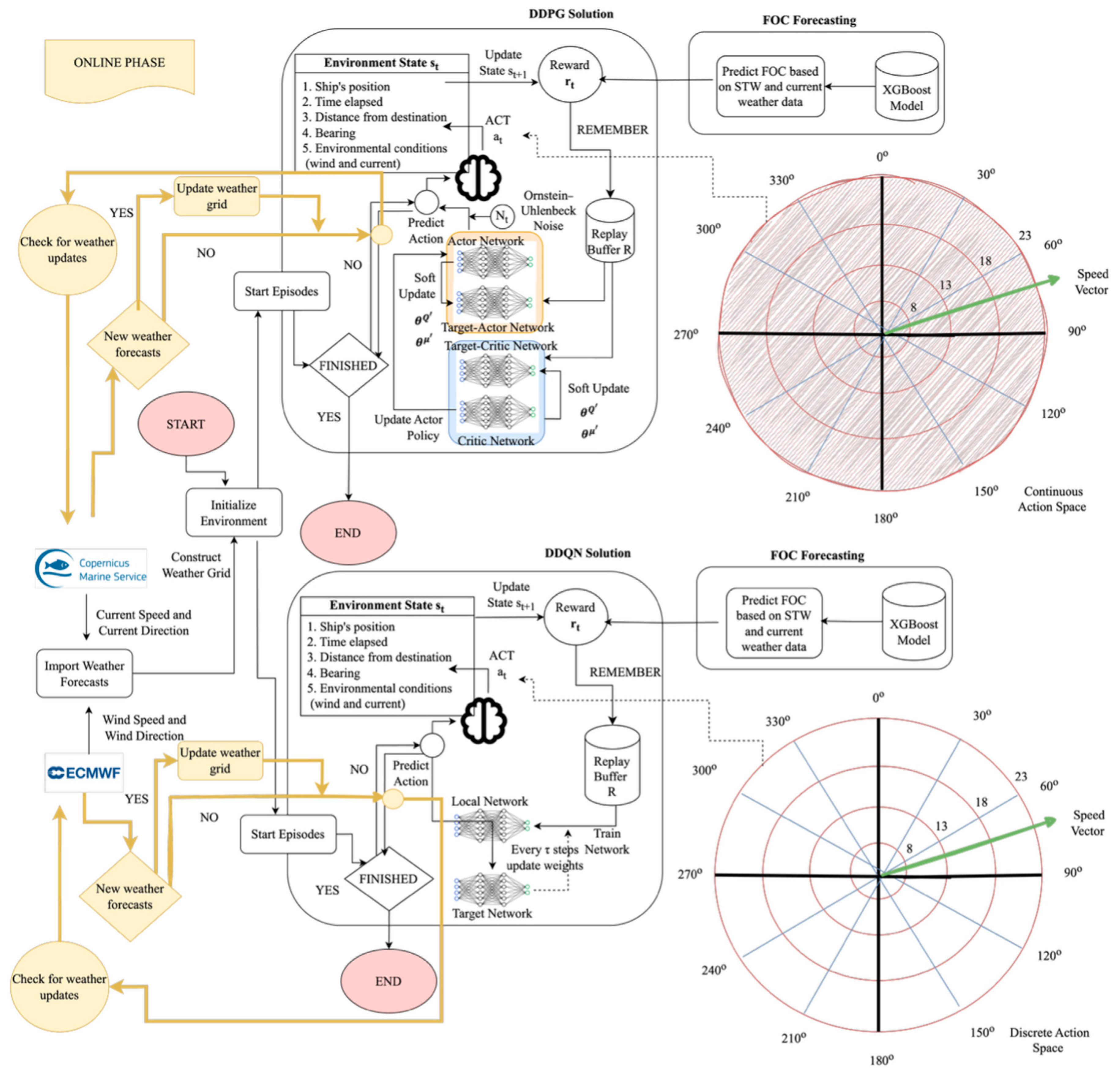
4.1. Simulation Environment

The DRL environment is defined by a grid system covering the smallest area that encloses both the departure and destination ports, with an additional buffer in each direction. This buffer prevents navigational challenges when ports are near land boundaries (Figure 1a). While the ship navigates continuously through the environment, each grid node is associated with expected weather conditions based on the ship’s ETA at that node. The grid resolution matches the 0.25° resolution of the weather data, presented later in this section, ensuring alignment between the environment and the data inputs.

The distance between two locations within the grid was calculated using the great circle distance derived from the haversine formula, ensuring accurate representation of the shortest path between two points on the Earth’s surface. The routing solution accounts for real-world navigational constraints, ensuring that the vessel stays within navigable waterways while avoiding obstacles like land or restricted zones.

To efficiently handle land obstacles, we adopted a “transparent” obstacle approach. Instead of immediately terminating an episode when the agent crosses land, which disrupts learning, the ship is allowed to pass over landmasses. However, a significant penalty was imposed in the reward function for any traversal of restricted areas. This method allows the agent to explore a wider range of potential routes without being constrained by abrupt terminations or inefficient course corrections. Over time, the agent learns that navigating through land results in lower cumulative rewards (High-Penalty Route in Figure 1b), which encourages it to find feasible water-based routes autonomously (Low-Penalty Route in Figure 1b). This approach enhances learning efficiency while ensuring that the vessel adheres to navigable waterways.

The state space represents the agent’s understanding of the environment and includes all essential information required for the ship to make informed decisions. To improve learning efficiency and avoid scale effects, the state variables are standardized and include the following:

• Geographical Position: The ship’s current coordinates (longitude and latitude).
• Elapsed Time: The time since the journey began, measured in seconds.
• Distance to Destination: The remaining distance to the target point.
• Environmental Conditions: Weather forecasts, including wind direction, wind speed, current direction, and current speed, interpolated based on the ship’s ETA.

To capture the dynamic nature of weather conditions, the weather forecasts were interpolated between the closest available timestamps, considering the ship’s projected arrival time at each grid node. ETA was calculated using a predefined routing profile (i.e., an average speed of 15 knots). Incorporating time as a state parameter ensures that the ship is at the optimal coordinates at the right time and simultaneously penalizes arrival times outside the optimal arrival time window.

The action space defines the ship’s controllable parameters: Speed Through Water (STW) and bearing. These parameters affect fuel consumption directly and indirectly by altering the ship’s position relative to prevailing weather conditions. Based on the selected DRL algorithm, the agent chooses its actions from discrete and continuous action spaces, respectively:

• Discrete Action Space (DDQN): The agent selects a bearing in the range of [0°, 180°], with intervals of 10°, and STW values between 8 and 22 knots with unit intervals. Most commercial vessels, such as bulk carriers, container ships, and tankers, typically operate within this speed range under normal conditions to avoid excessive fuel consumption and mechanical stress. Smaller intervals (e.g., 5°) for bearings were found to increase the likelihood of suboptimal policies due to insufficient exploration and an excessive number of alternative routes.
• Continuous Action Space (DDPG): The agent can select any bearing in the range of [0°, 360°) and any STW in the range defined for the discrete action space.

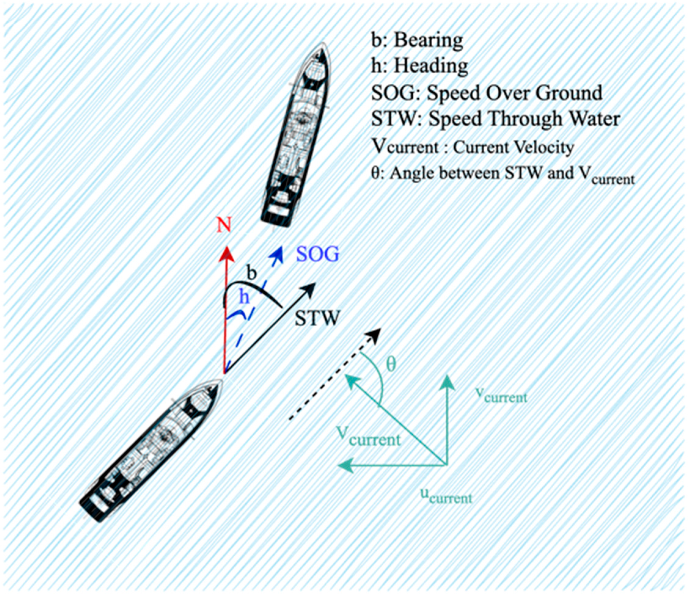
4.2. Problem Formulation

While the agent controls STW and bearing, calculating the next state (and subsequently the ship’s position) requires the Speed Over Ground (SOG) and heading as inputs. These values account for external weather conditions, so conversion is necessary. SOG (in miles/minute) is derived from STW by factoring in the effect of currents:

$$SOG=0.037\times (STW+V_{current}\times \cos \Theta \left(ST{W}_d, {Current}_d\right))$$

(1)

where

• $STW$ is the Speed Through Water (knots);
• $V_{current}$ is the ocean current velocity (m/s);
• $ST{W}_d$ is the ship’s movement direction;
• ${Current}_d$ is the current’s direction;
• $\Theta \left(ST{W}_d, {Current}_d\right)$ is the angle between the ship’s speed and current direction (degrees);
• 0.037 is a unit conversion constant (m/s to nautical miles per minute).

The current velocity and the current direction were calculated from the northward and eastward current components, as demonstrated in Figure 2.

Equation (1) explains how water currents either assist or hinder the ship’s progress relative to the ground. For example, if the ship is moving in the direction of the current, the two speeds are added, whereas, if it is moving in the opposite direction, they are subtracted.

The data available from Copernicus Marine Service provide the northward ocean current velocity $u_{current}$ in m/s and the eastward ocean current velocity $v_{current}$ in m/s. $V_{current}$ is calculated in the following way:

$$V_{current}=\sqrt{{u_{current}}^2+{v_{current}}^2}$$

(2)

while ${Current}_d$ is as follows:

$${Current}_d={\tan }^{-1}(u_{current},v_{current})$$

(3)

Heading is the actual direction in which the ship is moving, which may differ from the bearing due to external factors such as wind, currents, and other environmental influences. Therefore, the heading can be estimated by adjusting the bearing based on these environmental factors. A simplified relationship might involve solving the following:

$$Heading=Bearing+Drift\_Angle$$

(4)

where the drift angle accounts for the impact of wind and current forces that push the ship off its intended course, and it can be approximated as follows:

$$Drift\_Angle={\displaystyle \frac{WS}{SOG}}$$

(5)

where WS is the wind speed in knots. Therefore, we must solve a system of two equations (Equations (1) and (4)) with two unknowns: SOG and heading. The heading is indirectly expressed in Equation (1) within the cosine function. This system is solved with numerical optimization using a non-linear solver.

The reward at each step t is the core component guiding the agent toward energy-efficient and timely routing decisions. It evaluates actions based on multiple components:

• Dr: Reduction in the distance to destination. This encourages progress towards the destination by comparing the vessel’s current and previous Haversine distances to the target. This ensures timely feedback for every action taken.
• Pt: Penalty associated with travel time exceeding expected thresholds. It is applied when the vessel deviates from the ideal JIT arrival window.
• Ps: Speed penalty. This penalty ensures that the vessel operates at an optimal speed, minimizing fuel consumption while adhering to JIT constraints.
• P_O: Obstacle penalty. This is a large penalty that is applied if the vessel crosses an obstacle.
• $w_1,w_2,w_3:$ Weighting factors applied to each respective component.
• ${\delta }_o$: Boolean variable that is true if the ship crosses an obstacle (e.g., land).

The reward function is formulated as follows:

$$R_{\mathit{t}}=w_1{D}_r-w_2{P}_t-w_3{P}_s-{\delta }_o{P}_o$$

(6)

After extensive testing and calibration, we estimated the weights as follows: $w_1=1,w_2=2,\mathsf{a}\mathsf{n}\mathsf{d} w_3=3000.$ Pt is proportional to the time difference $t_{to\_destination}=t_{ideal arrival}-t_{current}$ relative to ideal time window $t_{ideal window}$ (Equation (7)), where $t_{to\_destination}$ is the time needed to arrive to the destination, $t_{ideal arrival}$ is the ideal time of arrival, $t_{current}$ is the current time of the simulation, and $t_{ideal window}$ is the ideal time window around the ideal time of arrival. This means that the longer the arrival is delayed beyond the ideal arrival time, the higher the penalty is and can be expressed as follows:

$$P_t=\left\{\begin{array}{c} 0 if t_{t{o}_{destination}}>0 \\ {\displaystyle \frac{\left|t_{t{o}_{destination}}\right|}{t_{ideal\_window}}} if t_{t{o}_{destination}}<0\end{array}\right.$$

(7)

For each possible speed, a machine learning (ML) model estimates the Fuel Oil Consumption (FOC) based on weather. The agent is penalized based on the deviation from the optimal speed $P_s=|{speed}_a-{speed}_{optimal}|$, where ${speed}_a$ is the actual and ${speed}_{optimal}$ is the optimal speed.

Penalties for approaching obstacles without collision were tested but led to undesired behavior near port areas. To mitigate this, “port entries” were defined instead of precise port coordinates, and the final parts of the journey were executed with predefined speed and trajectories.

The final reward function incorporates cumulative fuel consumption (FOC_Cum), JIT arrival incentives (R_JIT), and penalties for going outside the environment grid (P_OOB):

$$R=\left\{\begin{array}{c} R_a-{FOC}_{cum}+{\delta }_{JIT}{R}_{JIT}, if d_{t{o}_{destination}}\le {\epsilon }_{threshold }\\ { P}_{OOB }{d}_{to\_destination} if t_{current}=T and d_{to\_destination}>{\epsilon }_{threshold}\\ R_t otherwise \end{array} \right.$$

(8)

where

• $R$: Final reward.
• $R_a:$ Arrival reward.
• ${\delta }_{JIT}$: Boolean variable that is true if the ship arrives within the JIT constraints.
• $d_{t{o}_{destination}}$: Distance to destination.
• ${\epsilon }_{threshold}$: Acceptable distance range for successful arrival.
• T: Maximum allowable steps per episode.

Each simulation episode terminates under three conditions: (1) reaching the destination within a buffer zone around the target coordinates to prevent premature terminations and allow for more flexible maneuvering, (2) crossing environment boundaries, which triggers a penalty proportional to the remaining distance to the destination, guiding the agent to stay within permissible limits, and (3) exceeding the maximum threshold of iterations without reaching the goal, resulting in a distance-based penalty.

4.3. Phased Optimization Approach

The multi-objective routing optimization problem was tackled through a two-phase planning process: pre-voyage planning (offline phase) and real-time optimization during the voyage (online phase). In the first stage (offline), the DRL algorithm was trained offline using the initial weather forecasts, navigational constraints, and operational limits, under the assumption that expected conditions remain unchanged. The primary objectives during this phase are to optimize fuel consumption, ensure timely arrival, and adhere to predefined restrictions. The resulting policy represents an optimal route based on the forecasted weather patterns and known constraints. This pre-trained policy serves as a robust baseline, equipping the vessel with an optimal route and speed profile before departure. Once the voyage begins, the DRL framework transitions into phase 2, online adaptation. The initial route generated using early weather forecasts acts as the reference plan. However, as conditions change, the model continuously updates its decisions based on the incoming real-time data, including updated weather forecasts, current ship status, and newly identified restrictions/obstructions.

Weather updates were incorporated twice daily. These updates ensure that the route remains aligned with the most current forecasts, preventing outdated predictions from compromising efficiency during long journeys. The pre-trained offline model significantly reduces computational demands during this phase, as the algorithm fine-tunes existing policies rather than learning from scratch.

The relationship between the offline pre-training phase and the online real-time adaptation is illustrated in Figure 3. This figure highlights the additional components of the phased optimization approach, showing how it continuously checks for weather updates and dynamically adjusts the weather grid of the environment.

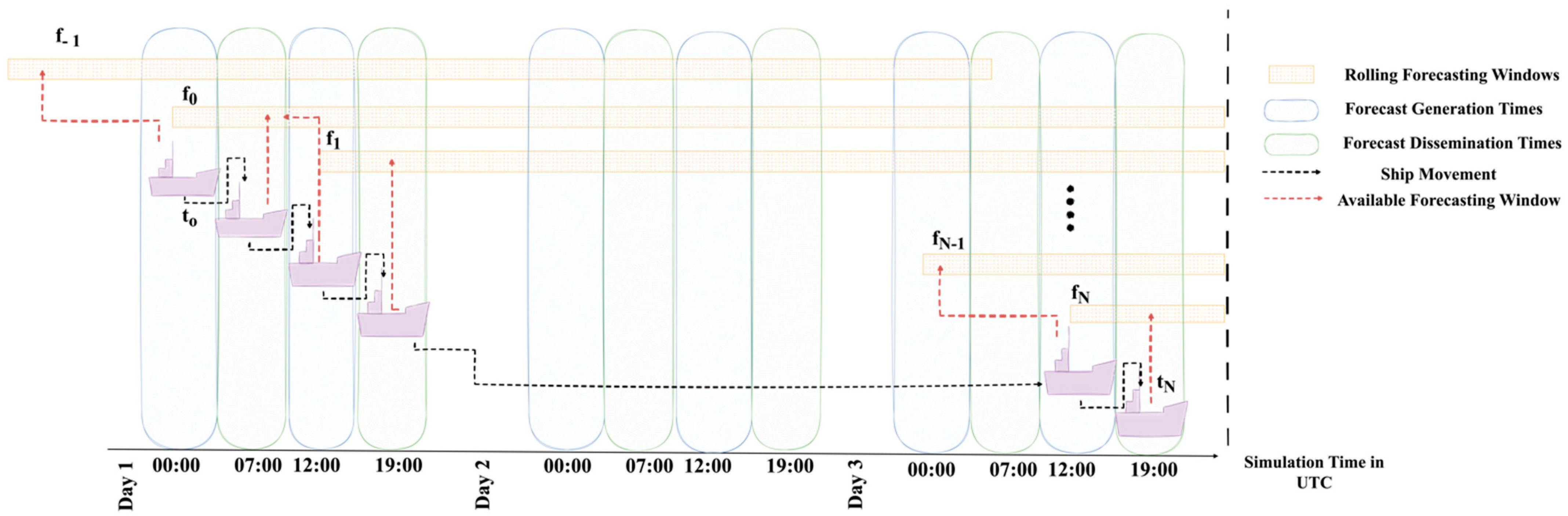
4.4. Weather Integration

Essential to the approach presented here is the integration of meteorological data and forecasts. The accuracy of weather forecasts is significant for the effectiveness of weather routing. Short-term weather forecasts are accurate for up to two weeks and provide crucial information about waves, currents, wind, and temperature. Long-term predictions are less precise but still valuable for strategic planning. Some researchers suggest using ensemble forecasts to capture variability in weather development and improve the robustness of selected routes.

For this study, we used weather data from the Copernicus Data Store (CDS), managed by the European Centre for Medium-Range Weather Forecasts (ECMWF). CDS offers free and open access to a wide range of climate datasets and tools. A key source is the ERA5 reanalysis dataset, which provides hourly estimates of atmospheric, oceanic, and land-surface variables at a horizontal resolution of 0.25° × 0.25° (approximately 31 km globally). This dataset combines historical observations with numerical weather prediction (NWP) models, ensuring a consistent and comprehensive time series of environmental conditions, including temperature, precipitation, wind speed and direction, pressure, and humidity.

In addition to ERA5 reanalysis, ECMWF provides real-time weather forecasts critical for applications requiring up-to-date atmospheric conditions. These forecasts are generated four times daily—at 00, 06, 12, and 18 UTC (Coordinated Universal Time). However, only the 00 and 12 UTC forecasts extend 240 h into the future, while 06 and 18 UTC forecasts cover only 90 h. For this reason, the 00 and 12 UTC forecasts were prioritized for the weather routing implementation. The forecast data, disseminated seven hours after generation (e.g., 07 UTC for the 00 UTC run), were retrieved using the ECMW API (Application Programming Interface) client and cached to avoid redundant processing.

For the online phase of the voyage optimization, rolling forecasting windows were employed (Figure 4). Every 12 h, the forecasting window was updated from f₀ to f_N where N is the number of 12 h steps in the simulation, and it looks forward for M steps in the future where M is defined based on the duration of the journey. Two different types of zones are demonstrated: the time zones when forecasts are generated, and the time zones where forecasts become publicly available. For example, at 07:00, when the forecasts for 00:00 are disseminated, the ship is using the respective forecasting window. The same applies for 12:00, because, while the new forecasts were generated, they are still not disseminated until 19:00. In the beginning of the journey, t₀, it is necessary that the ship employs a forecast f₋₁ that was generated in the past. To ensure seamless integration into the routing environment, the 3 hourly forecast data were interpolated to hourly intervals using a weighted average based on the time difference between the target hour and the surrounding 3 h steps. This approach assists in maintaining temporal continuity.

In addition to wind data, ocean current speed data were sourced from the Copernicus Marine Service (CMS). Since the CDS does not provide this information, we used the Global Ocean Physics Analysis and Forecast dataset [42], which offers over 30 variables such as salinity, currents, and potential temperature among others. The variables of interest for this study are the vertical and horizontal components of the 10-day forecasts for hourly mean sea currents at a resolution of 1/12°, which is a higher granularity than the atmospheric data. This dataset was updated daily.

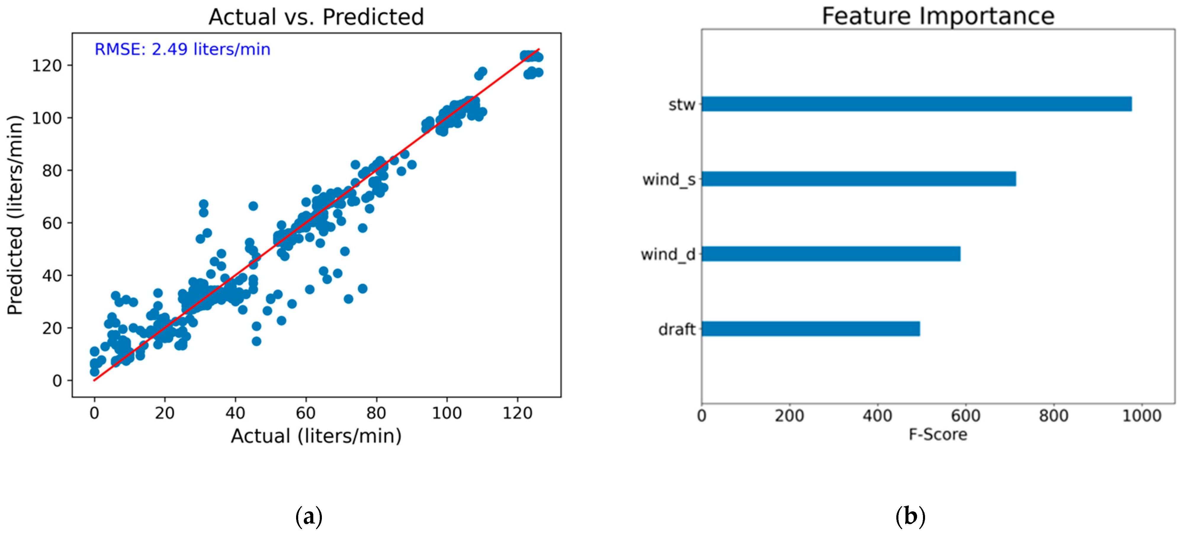
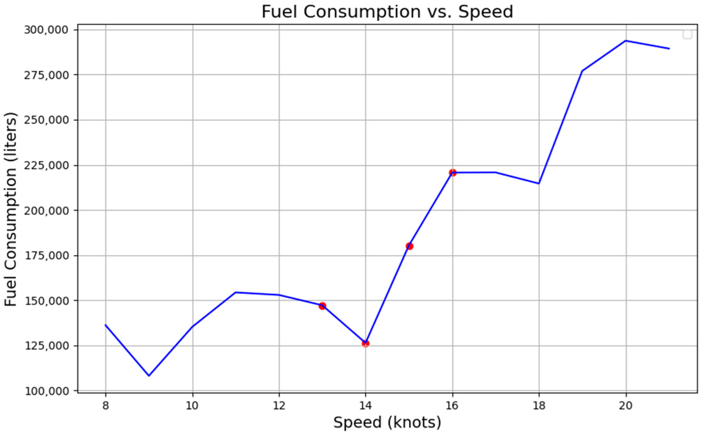
4.5. Fuel Oil Consumption (FOC) Modeling

Fuel consumption is a critical concern in shipping, particularly as it relates to cost and environmental impact. Weather routing can lead to significant fuel savings, typically reported between 3% and 5% per voyage. However, the extent of these savings depends on the methodologies used in fuel consumption prediction models. Traditional approaches often rely on empirical models, which may oversimplify the complex interplay between vessel performance and external factors such as wind, waves, and currents.

The factors influencing fuel consumption during a voyage can be broadly categorized into ship operation factors and environmental variables [43]. Ship operation factors include speed, main engine power, draft–trim configuration, hull roughness, and displacement, all of which directly affect the ship’s hydrodynamic performance. Environmental variables, on the other hand, include wave direction and height, wind force, temperature, currents, and even salinity, each of which can impose additional resistance on the vessel, altering its fuel consumption. Capturing the combined effects of these diverse factors is essential for accurately predicting fuel usage, yet the complexity of their interactions makes this a challenging task.

Recent advancements have seen the rise in machine learning-based models, which excel at capturing non-linear relationships in high-dimensional datasets. These models integrate diverse inputs—such as ship speed, draft, trim, and high-resolution meteorological data—to improve predictive accuracy [44]. Artificial neural networks (ANNs) are particularly prominent in this domain, as they iteratively learn from collected data, adjusting the weight of each parameter to simulate the intricate relationship between fuel consumption and external conditions. By fusing real-time sensor readings with weather forecasts, these models transform absolute meteorological variables into relative information meaningful for fuel efficiency analysis, such as wind and wave conditions relative to the ship’s heading [45].

In this study, we employ an ML approach using an XGBoost Regressor v.2.1.4. This predicts fuel consumption in liters per minute (L/min) based on a feature set collected from onboard sensors, provided by Danaos Shipping Co., Ltd. (Piraeus, Greece). Key features include STW, ship draft, wind speed, and wind direction. The STW and wind conditions are dynamic, but we assumed a constant ship draft over the course of a journey, as it mainly depends on the vessel’s characteristics (e.g., weight, hull shape, waterplane area) and the seawater density, which is relatively stable.

The XGBoost model achieved a Root Mean Squared Error (RMSE) of approximately 2 L/min, reflecting a good fit based on the FOC distribution in the training dataset (Figure 5a). During data preprocessing, instances where the speed was below 8 knots were excluded, as these were primarily associated with port operations, maneuvering, or anchoring. This filtering reduced the dataset size by approximately 60%. Feature importance analysis (Figure 5b) revealed that STW was the most influential predictor, followed by wind speed. The model, configured with a learning rate of 0.1 and a maximum depth of 5, was trained on 80% of the dataset and tested on the remaining 20%.

The XGBoost model was seamlessly integrated into the DRL environment, providing real-time fuel consumption predictions at each decision step. Moreover, the DRL-XGBoost model accounts for wind speed and direction when predicting fuel consumption, aligning with the limitations of the available data. Although wave-related effects are not explicitly modeled, they are partially captured through the wind features. The flexible structure of the XGBoost model allows for the future inclusion of additional weather variables as more comprehensive datasets become available.

Looking ahead, the XGBoost component could potentially be replaced by more advanced models, such as LSTM. That would incorporate autoregressive terms from previous journey steps, potentially enhancing forecasting accuracy.

4.6. Computational Setup

All computations were carried out on a laptop equipped with an Apple M1 Pro chip (10-core CPU, 16-core GPU), with 32 GB of unified memory. While GPU acceleration was available, Deep Reinforcement Learning (DRL) methods exhibited minimal performance improvement compared to CPU execution, largely due to communication overhead between the environment and the learning networks. Experiments were implemented in Python 3.12 using tensorflow 2.16.1.

5. Results and Discussion

5.1. Results

To evaluate the performance of the DRL solutions, we selected a scenario in the Mediterranean, representing a shipping route (Marseilles to Piraeus) where weather conditions, geographical constraints, and JIT arrival requirements can significantly impact voyage optimization. This route was chosen for its strategic importance and geographical variety, as it spans diverse maritime zones from the western Mediterranean to the Aegean Sea. It was selected to test a scenario typical of the types of vessels involved in commercial shipping in the region. An additional reason for selecting this route was that it introduces complex geographical challenges, particularly in navigating through confined waterways, which is less commonly addressed in the literature to present.

The selected vessel for this study is a typical medium-sized container ship. The ship’s propulsion system is assumed to be conventional diesel, which simplifies the model and ensures that this study’s objectives are not overwhelmed by the added complexity of newer vessel technologies (e.g., dual fuel types, data availability, etc.).

This scenario (Figure 6) includes the challenge of navigating through constrained environments, such as the Corinth Canal. Given the complexities of passing through such narrow, confined areas, where both the canal’s structure and maritime regulations limit flexibility, it is unrealistic to expect DRL algorithms to optimize both navigation and fuel consumption simultaneously. Not only is there limited room for weather routing within the narrow confines of the canal, but real-world constraints such as port authority regulations, ship traffic, and priority systems further limit navigation options. To address this, we introduced a “teleportation” mechanism. When the ship approaches the entry point of the canal, it is automatically “teleported” to the exit, following a pre-defined trajectory at a constant speed (Figure 7). The DRL algorithm resumes optimization once the ship exits the canal. This simplification has minimal effect on the overall results.

The buffer zones around the destination and teleportation zones are set to 20 km, allowing flexibility as the vessel approaches the destination. The simulation time step is 60 min. To accommodate the extended travel time, we assumed that the JIT arrival window corresponds to a 10 h range. The action space for the heading of the vessel has angular increments of 10°, balancing computational efficiency with path optimality. Finally, the environment grid resolution was reduced from 0.25° in the weather data to 1.00° to enhance processing efficiency while maintaining essential weather pattern resolution.

Data between 09-03-2025 and 12-03-2025 were used for the training of the models, and data from a different time window (28-03-2025 to 31-03-2025) were used to fine-tune and evaluate the models under different conditions. As discussed in Section 4.4, the presented approach has an offline and an offline phase. The DRL algorithms are evaluated for both the offline phase (Section 5.1.1 and Section 5.1.2) and the online phase (Section 5.1.3). In Section 5.2, several voyage optimization solutions are explained, which this research has implemented to benchmark the DRL solutions. This includes A* search, Hill Climbing, Tabu Search, and Adaptive Large Neighborhood Search (ALNS). All algorithms, including the DLR ones, are also compared against a distance-based baseline solution (see Section 5.2.1) referred to as the “baseline model”, so relative performance can be established and ranked.

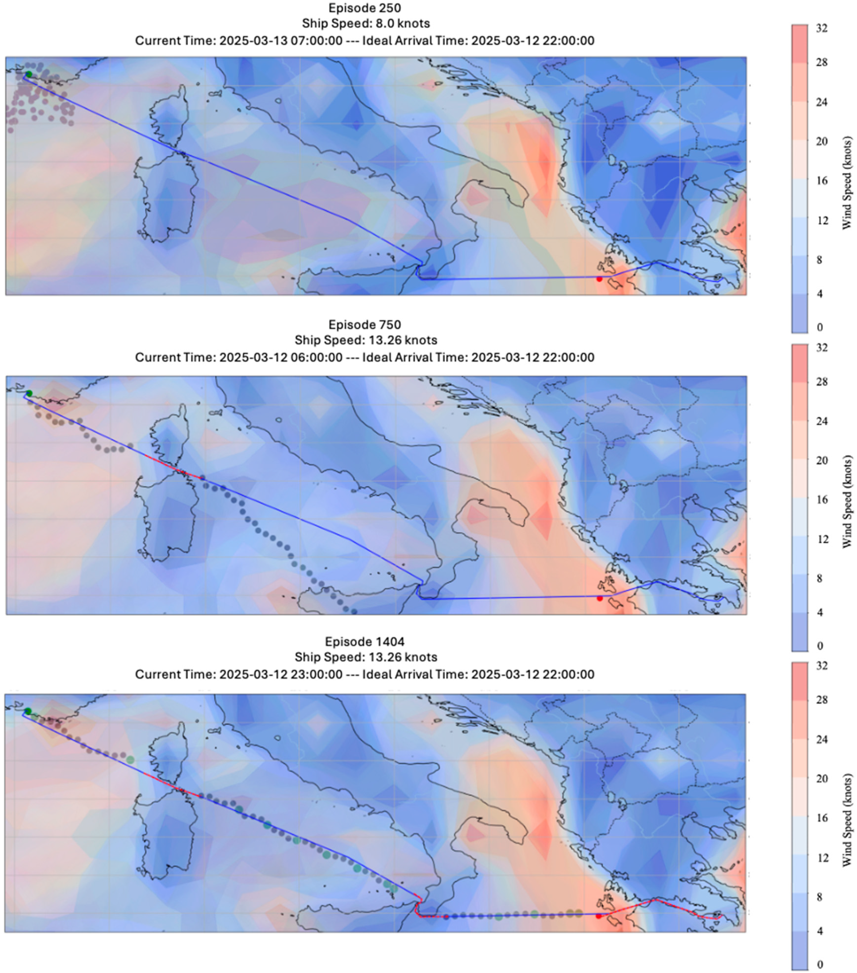
5.1.1. DDQN Results

Here, we present the results from the offline algorithm phase. The evolution of how the agent learns to navigate throughout the DDQN scenario can be seen in Figure 8.

After 250 episodes, the ship is still randomly moving around the environment, and it reaches the maximum threshold of iterations before the episode is terminated. In episode 500, the ship movements are still quite noisy, and the ship again reaches the maximum threshold of iterations; however, this time, it learns to cross the first “teleportation” area between Corsica and Sardinia. This happens because the reward function is heavily based on the reduction in the distance between the ship and the trip destination. Since the “teleportation” performs multiple 60 min steps at once, the distance reduction is stronger than any other move; therefore, the ship learns to avoid the obstacles.

Finally, near the end of training (at 1498 iterations), the ship learns to follow optimal behavior. It manages to cross the second “teleportation” area between mainland Italy and Sicily, and, then, it reaches the destination at the Ionian Sea, from which point on, it follows the shortest path trajectory until the port of Piraeus. It also moves with a speed of 14 knots for the largest part of the route, whereas, in the “teleportation” areas, the assumption is that it moves with a speed of 9 knots. The final trajectory is smoothed. The smoothing process works by checking if consecutive waypoints in the path can be directly connected without crossing land. If a valid direct connection exists, the intermediate waypoints are removed, simplifying the route. Apart from shortening the path, this approach also minimizes abrupt course changes.

The DDQN model achieved 8.7% FOC reduction compared to the baseline model. More detailed results in terms of fuel consumption, voyage time, and speed profiles will be presented in Section 5.2, where the DRL approaches are compared to other heuristics.

The DRL algorithms can be unstable when there are changes in the environment. Specifically, when we tried to perform weather routing with the trained model on a different day, changes in wind and current speed and direction affected the optimal routing strategy. The pre-trained model led to a suboptimal solution where the ship ends up far away from the destination. By fine tuning the existing model on the new environment (Figure 9), we successfully adapted the routing policy to account for these variations, going through the teleportation areas and reaching the destination.

The fine-tuning required only 130 episodes to obtain the optimal solution, which is much faster than the pre-training stage. The reduction in FOC compared to the baseline solution is comparable to the reduction for the original day (7.9% for the new day vs. 8.7% for the original one). Our approach demonstrates that, rather than retraining the model from scratch for every new scenario, there is an option to retain a single model per route and fine-tune it for different days, resulting in a more efficient and scalable solution.

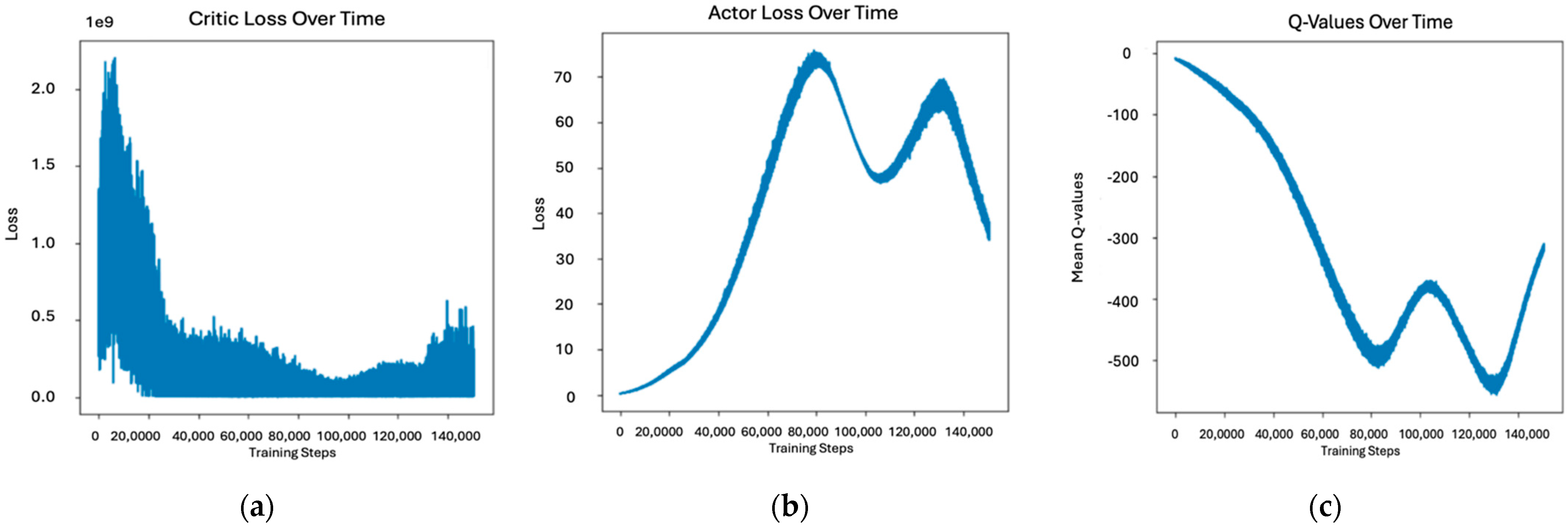
5.1.2. DDPG Results

The training dynamics of the DDPG algorithm for the offline phase are illustrated in Figure 10. Initially, the critic loss (Figure 10a) is high, as expected, since the model starts with random weights and struggles to evaluate actions correctly. As training progresses, the loss steadily declines, indicating improved performance in value estimation. The oscillatory patterns around 90,000 and 130,000 steps suggest adjustments in policy learning as the agent explores and refines its decision-making strategy. The same applies to the actor loss (Figure 10b), which represents the error in the policy network, and to the Q-values (Figure 10c), which represent the estimated future reward. The increase at the end suggests that the agent is learning to predict increasingly better rewards, making more informed decisions.

This process is better illustrated in Figure 11 where we observe the ship’s path evolving over the course of training with the DDPG algorithm. Due to the continuous action space and the application of Ornstein–Uhlenbeck (OU) noise, the adjustments in speed and direction are small and smoother compared to the abrupt changes in the DDQN. As a result, exploration takes longer, and the agent initially struggles to find an optimal path.

The agent is allowed to move in a [0°, 360°) range; hence, after 250 episodes, it looks like it is still moving randomly around the starting point. In a similar way to the DDQN, the agent first learns to cross the first “teleportation” area; however, in this case, it needs more episodes (approximately 750, instead of 500) to reach that milestone.

Around 1300 episodes, we see a marked improvement. The agent starts to consistently find the correct path while making incremental speed adjustments. The ship’s speed remains within a reasonable range, and the path becomes more direct. At this point, the DDPG agent learns the general direction towards the destination and focuses on optimizing its speed, a behavior that is in line with the training dynamics in Figure 10.

This gradual refinement reflects the way OU noise works in the DDPG example. While this model does not have the DDQN’s ability to abruptly switch between discrete speeds within a single episode, it achieves higher levels of optimality by exploiting the marginal improvements from the continuous action space. In particular, the algorithm results in a speed that oscillates between 13 and 14 knots across the journey, and it achieves a 12.6% reduction in FOC compared to the baseline model. The marginal adjustments in angle between consecutive episodes compose a trajectory that is already quite smooth, but, at the same time, the smoothing process has a strong impact on FOC because it eliminates unnecessary maneuvers.

As with the DDQN, applying the trained DDPG model to a different day led to suboptimal results due to changes in wind and current conditions. After updating the weights of the existing model, the policy successfully adapted to account for these variations. Fine tuning required 250 episodes—significantly faster than full retraining—while maintaining a similar FOC reduction of 12.1%.

These results show that, for both the DDQN and DDPG, while the direct application of the pre-trained model to a different environmental dataset may initially yield suboptimal or even erroneous routes, updating model weights leads to consistent performance improvements.

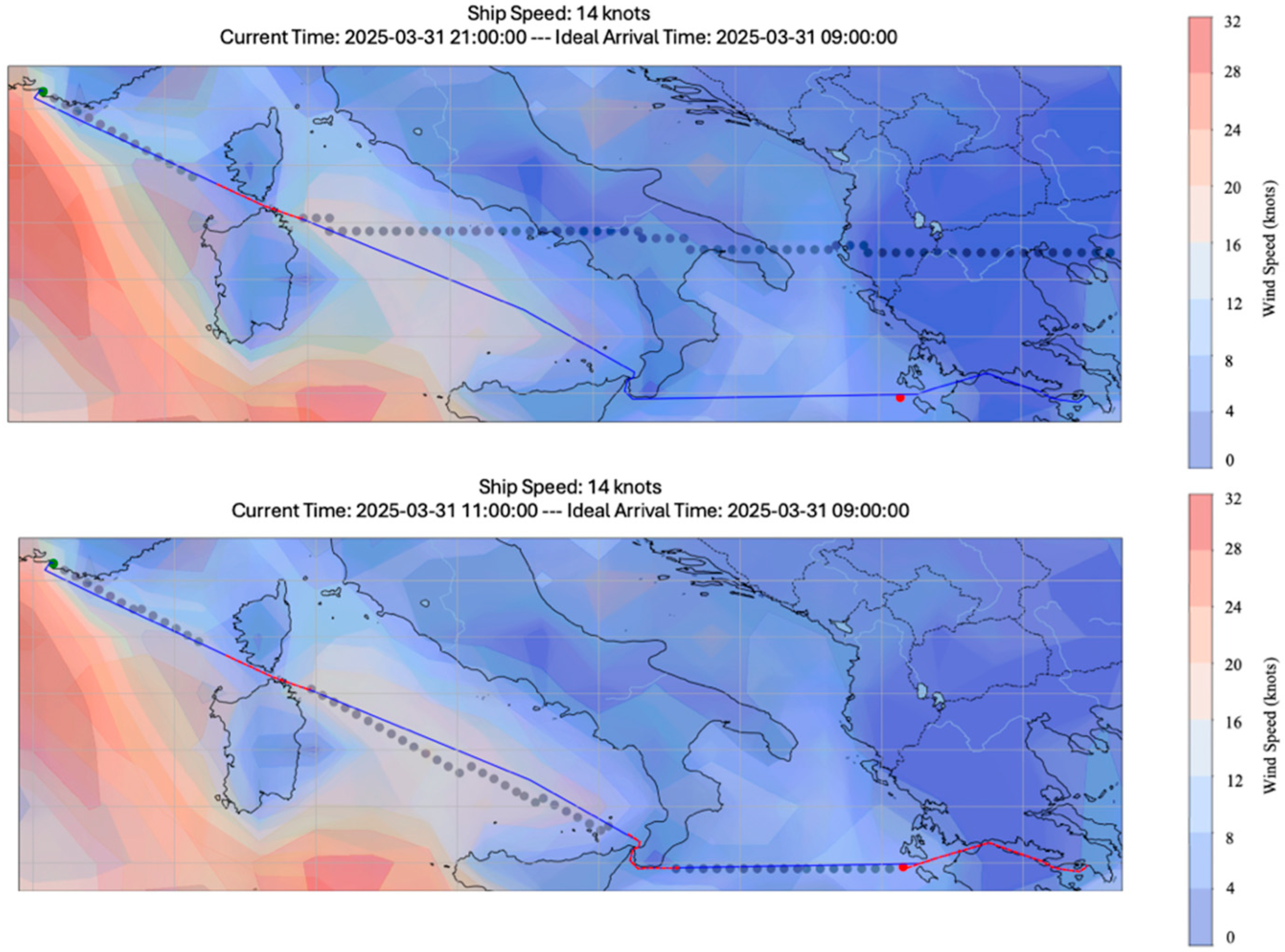
5.1.3. Adaptation to Real-Time Weather

In the offline phase, weather forecasts from the ECMWF are acquired at the start of the journey and projected into the future, informing the model about anticipated wind speed and direction—critical variables for routing decisions. A limitation of the open-access dataset is that forecasts are only available for up to three days in the past, which is sufficient for the Marseille–Piraeus journey but would require the development of a historical database for training models on longer itineraries.

To address forecast aging during the voyage, we dynamically update the weather grid based on the ship’s estimated time of arrival (ETA) at each grid point, retrieving the most relevant forecasts. However, over longer durations, initial forecasts progressively lose accuracy, making regular updates essential to maintain routing precision.

In the online phase, the DRL model initially trains with the available forecast set. As the simulation clock progresses, it automatically detects forecast dissemination times, downloads the latest weather data, regenerates the weather matrix (latitude, longitude, and time), and updates the routing environment accordingly. These environmental shifts during an episode may render the initial model weights suboptimal, potentially affecting navigation success.

To counter this, we further adjust the model weights during the simulation, improving its adaptation to updated conditions. As shown in

Table 2. Performance comparison of online vs. offline models under dynamic weather updates.

	DDQN (Offline Policy)	DDQN (Online Policy)	DDPG (Offline Policy)	DDPG (Online Policy)
Fuel Consumption Reduction (%)	6.6	8.3	10.7	11.9

, when re-evaluating the original routing policy under updated forecasts, fuel consumption savings dropped to 6.6% for the DDQN and 10.7% for the DDPG, reflecting a performance decline but providing a more realistic estimate, as real-world weather is more likely to resemble the latest forecast. After online weight adjustment, fuel savings improved to 8.3% (+1.7%) for the DDQN and 11.9% (+1.2%) for the DDPG, demonstrating the advantages of real-time adaptation.

5.1.4. Hyperparameter Tuning

Hyperparameter tuning plays a crucial role in the performance of DRL models. For both the DDQN and DDPG, we performed an extensive search over key hyperparameters, leveraging both grid search and manual tuning. The primary goal was to achieve optimal solutions and, at the same time, enhance the model’s stability and minimize oscillations in the loss functions. The detailed final specifications of the two models, as well as the adjustments made when fine tuning the models for different days and real-time weather data, are presented in Appendix A.

5.2. Benchmarking

Benchmarking in weather routing has long been hindered by the lack of standardized optimization problems, making direct comparison between algorithms challenging [46]. Studies often use unique origin–destination pairs and different departure dates, leading to distinct optimization scenarios. Additionally, the wide range of reported emission savings could be narrowed by establishing baseline cases, offering benchmarking instances and conducting sensitivity analyses—for example, examining the impact of environmental data resolution [11]. Recently, de la Jara et al. [47] introduced WeatherRoutingBench 1.0, which provides a standardized set of problem instances that specify origin, destination, and other relevant conditions, thus enabling more systematic performance evaluations.

Establishing a robust benchmark is essential when evaluating the performance of DRL, as the benchmark will enable us to assess the efficiency and effectiveness of DRL-derived routes against theoretical optimal or near-optimal solutions.

In this subsection, we first describe the baseline route used for benchmarking, followed by an introduction to the H3 grid system, which underpins all benchmarking methods (A*, Hill Climbing, Tabu Search, and ALNS). We then describe the implementation of these methods as adapted to the maritime weather routing problem. These algorithm implementations incorporate several problem-specific features, such as fuel consumption modeling, trajectory smoothing, and arrival time constraints. After describing the methods, we present the results of their comparative performance evaluation.

5.2.1. Shortest Path Based on Maritime Graph

The simplest and most intuitive approach to benchmarking the DDQN and DDPG solutions was to use the shortest maritime path between the origin and destination port as a baseline. This path was computed with the scgraph 2.1.0 Python package, which applies a modified Dijkstra’s algorithm and the Haversine formula to account for the curvature of the Earth. This path is derived from the Global Shipping Lane Network [48], which is enriched with AIS-based routes around European coasts, enabling the realistic modeling of frequent maritime paths. Fuel consumption along this weather-agnostic route is calculated for various speeds, selecting the minimum consumption configuration as the optimal baseline. While this approach excludes weather conditions, it provides a useful reference line for evaluating DRL performance.

Figure 12 illustrates the total FOC in liters when the ship follows the shortest path at different speeds.

In Figure 12, speeds lower than 13 result in late arrivals, and speeds higher than 16 result in early arrivals, both incurring penalties. The optimal speed to minimize FOC is 9 knots, but, accounting for JIT arrival, it becomes 14 knots with a respective consumption of 126,382 L.

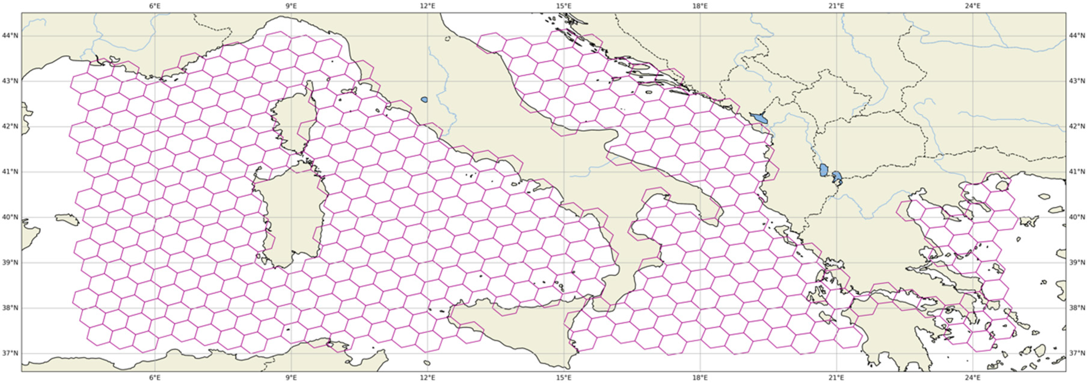
5.2.2. Grid-Based Benchmarks—The H3 Grid

While the DRL solutions are grid-agnostic with respect to vessel movements, the majority of the existing routing solutions inherently rely on a grid structure to explore possible paths. Typical square grids like the Mercator Projection have limitations due to Earth’s spherical shape, which needs to be distorted to fit the grid. In this study, the H3 hexagonal system [49] was selected as the spatial discretization method as in the study of [47]. H3 is a hierarchical geospatial indexing system that partitions the Earth’s surface into hexagonal cells (Figure 13), offering several advantages for modeling ship routes:

• Uniform Connectivity: Each hexagon has six neighbors, ensuring consistent connectivity throughout the grid, which simplifies pathfinding and avoids the distortions caused by square grids.
• Isotropic Representation: Hexagons reduce directional bias, providing a more accurate representation of movement in all directions—a critical factor in maritime navigation.
• Multi-Resolution Analysis: H3 supports multiple resolution levels spanning from 1 m² (level 15) up to 4 × 10⁶ km² (level 1), allowing the grid’s granularity to be tuned according to the problem’s complexity and computational limits.

For the selected route, a resolution of level 4 was selected, which corresponds to hexagons with an edge of 22.6 km and a total area of 1770 km². At this level, the hexagons are coarse enough to reduce computational complexity while still providing a sufficiently detailed representation of the environment. A finer grid of level 5, with an edge length of 9.8 km and a total area of 253 km² led to suboptimal solutions due to the increased search space and the limited capacity of heuristics to efficiently explore all paths.

All the search algorithms and heuristics presented in the remainder are based on this hexagonal grid. As depicted in Figure 14, the hexagons where the centroids correspond to land were removed. Only those necessary for the completion of the route (i.e., near “teleportation” areas) have been manually retained and included in the search space together with the sea hexagons.

5.2.3. A* Search

The A* algorithm was implemented to find optimal routes while considering either distance or fuel consumption as the primary cost function. Initially the algorithm optimized purely for distance, serving as an initial solution for other approaches that explore local optima. This approach used the Haversine distance between hexagon centers. To improve operational efficiency, a fuel-consumption-based variant was introduced.

A* is a widely used pathfinding algorithm that is theoretically based on the Bellman equation and optimality as the cost function is a combination of the current state (the path so far) and all possible future states depending on the current. It operates by combining these two factors into a total cost function, where $g\left(n\right)$ represents the accumulated cost from the start to the current node, and $h\left(n\right)$ is a heuristic that estimates the cost from the current node to the goal. In our implementation, $g\left(n\right)$ captured the fuel consumption up to the current hexagon, while $h\left(n\right)$ projected the fuel required to complete the journey, considering forecasted weather conditions and assuming a constant speed. The algorithm then prioritized nodes with the lowest total estimated cost:

$$f\left(n\right)=g\left(n\right)+h\left(n\right)$$

(9)

Since estimating future fuel consumption along the path was computationally intensive, especially with fine-grained H3 hexagons, caching mechanisms were introduced to improve runtime efficiency. First, weather data were precomputed for all hexagons and times to avoid querying weather conditions repeatedly during pathfinding. Moreover, fuel consumption from each hexagon to the target hexagon was precomputed for a range of discrete speed values.

The resulting path can sometimes be overly complex, with unnecessary waypoints that make navigation less efficient. To address this, a smoothing function is applied after A* to reduce the number of waypoints. The smoothing process works in the same way as it was described for the DDQN algorithm.

Finally, constraints in the model ensure that the vessel adheres to operational limits. In particular, the algorithm enforces a time window, so that the vessel arrives within the designated time frame. Unlike the DRL approach, where the JIT arrival works as soft constraint, here and in the following heuristics, this acts as a hard constraint.

5.2.4. Hill Climbing

The Hill Climbing algorithm employed in this study is a greedy, iterative method aimed at minimizing fuel consumption along the ship’s route by incrementally improving the path and speed configuration. The process begins with an initial path and speed profile, generated by the distance-based A* shortest path. From this starting point, the algorithm iteratively explores neighboring solutions. Each iteration applies one of three strategies to generate neighboring solutions: (1) removing a hexagon from the path to shorten the route, (2) adding a new hexagon to explore alternative trajectories, or (3) adjusting the vessel’s speed along a segment of the journey. To enhance exploration, the strategy is selected randomly at each step. Additionally, multiple neighbors are explored per iteration to reduce the likelihood of prematurely converging to suboptimal solutions.

To mitigate stagnation in local optima, the algorithm incorporates a random restart mechanism. If no improvement is observed after a predefined number of iterations, the algorithm resets the path and speed configuration, injecting diversity into the search. This process repeats until either the maximum number of iterations is reached, or no further improvement can be found.

Incorporating random restarts partially mitigates the risk of becoming trapped in local optima; however, the algorithm remains inherently greedy, prioritizing short-term improvements over a more extensive exploration of the solution space.

5.2.5. Tabu Search

Tabu Search is a metaheuristic optimization technique that guides a local search procedure to explore the solution space beyond local optima, by using a “tabu list”, which temporarily restricts certain moves. It has the potential to work well in weather routing because it can efficiently navigate the high-dimensional space of potential ship paths and speeds while avoiding revisiting previously explored suboptimal solutions. Unlike traditional local search methods like Hill Climbing, which risk getting trapped in local minima, Tabu Search maintains a memory structure (i.e., the Tabu list) that prevents cycling and promotes exploration.

The process begins with an initial path and speed profile, generated by the distance-based A* shortest path. Each iteration of the algorithm generates neighboring solutions by applying perturbations to the current path and speed profile, based on the same three strategies described for Hill Climbing.

To guide the search towards optimal solutions, each neighboring solution is evaluated based on fuel consumption and travel time, ensuring that only feasible solutions respecting navigational constraints and time windows are considered. The best non-Tabu neighbor is selected as the new current solution, with the Tabu list dynamically updated to maintain a fixed length. The process continues for a predefined number of iterations or until convergence criteria are met.

5.2.6. Adaptive Large Neighborhood Search (ALNS)

Adaptive Large Neighborhood Search (ALNS) is a heuristic optimization method that extends the Large Neighborhood Search (LNS) approach by incorporating adaptive mechanisms to dynamically select the most effective operator during the search process. ALNS is well suited for combinatorial optimization problems with large solution spaces.

One of the key benefits of ALNS lies in its ability to balance diversification and intensification throughout the search process. Diversification ensures that the algorithm explores different areas of the solution space, while intensification focuses on refining promising solutions. ANLS achieves this balance by employing a set of “destroy and repair” operators to partially disrupt the current solution and rebuild it, with operator selection guided by adaptive weights. This resembles the exploration–exploitation strategy that is followed with DRL.

The implementation of ALNS begins by initializing the solution with the A* distance-based shortest path. The destroy and repair set selectively modifies portions of the path and speeds using one of the three following operators: remove hexagon, add hexagon, and generate random speed. The operators have the same logic as the three strategies followed in Hill Climbing and Tabu Search earlier.

To guide the search, ALNS employs an adaptive mechanism that dynamically updates operator weights based on their past performance. Successful operators that yield better solutions receive increased weights, enhancing their likelihood of selection in subsequent iterations, while less effective operators have their weights reduced.

The evaluation of each modified solution involves simulating the vessel’s journey along the proposed path with adjusted speeds. The algorithm assesses the resulting fuel consumption and travel time, and a greedy acceptance criterion is applied, wherein the newly generated solution replaces the current best if it achieves lower fuel consumption.

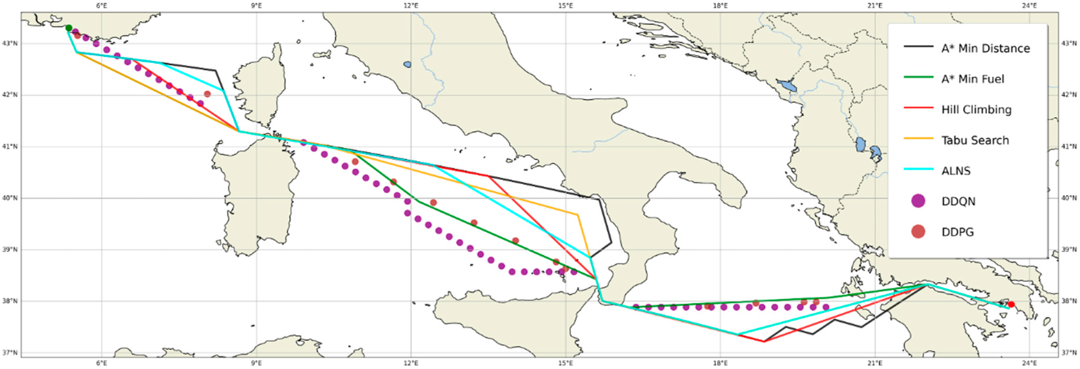
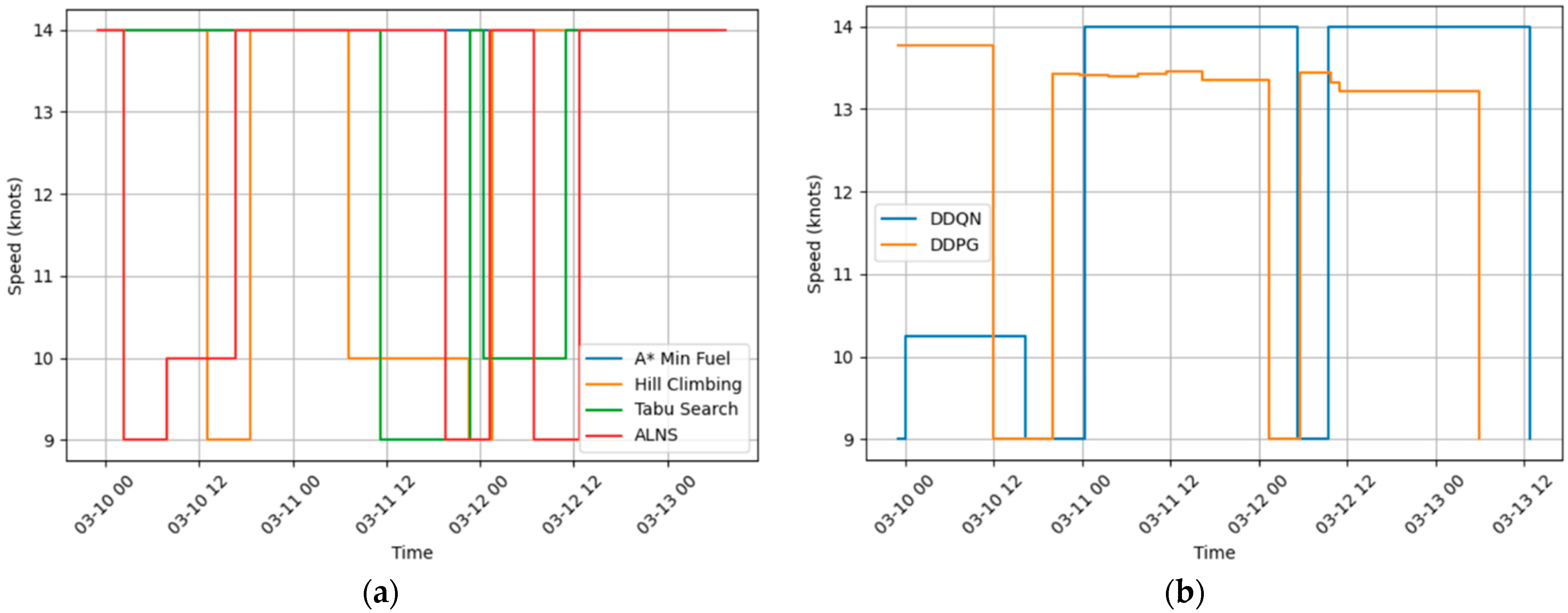
5.2.7. Algorithm Comparison

All the heuristics tend to produce similar ship courses (Figure 15), as the waypoint generation process follows a consistent structure across methods. Much like in systems based on orthogonal grids and great circle reference routes, the hexagonal framework imposes a uniform spatial discretization, guiding the algorithm towards comparable solutions despite differences in their optimization techniques. Nevertheless, this also applies for the DDQN and DDPG algorithms, where the generated paths exhibit similar patterns. Notably, the DDPG algorithm’s path follows very closely the A* minimum fuel path.

While the discretization of the search space results in routes with abrupt turns, which are impractical for real-world applications, the smoothing applied after A* as well as the operators applied for the other algorithms (e.g., the removal of intermediate waypoints) results in smoother trajectories.

The comparative analysis shown in

Table 3. Comparison of weather routing algorithms.

Method	Computation Time (s)	Fuel Consumption (Liters)	Average Speed (Knots)	Voyage Time (Hours)	Memory Usage	Adaptability to Weather	Applicability to Digital Twins
Graph-based Shortest Path (baseline)	3.2 s	126,382	14 *	71.0	Low	Low	Low
Distance-based A* Search	15.6	137,553 (+8.8%)	14 *	78.2	High	Low	Moderate
Fuel-based A* Search	462	122,903 (−2.8%)	14 *	69.1	High	Low	Moderate
Hill Climbing	143	119,130 (−5.7%)	11.62	79.9	Low	Low	Low
Tabu Search	150	108,946(−13.8%)	13.58	77.4	Moderate	Moderate	Moderate
ALNS	128	114,178 (−9.7%)	12.67	80.9	Moderate	High	High
DDQN	11,040 (920 for online)	115,346 (−8.7%)	12.30	85.8 **	Very High	Very High	Very High
DDPG	11,700 (1854 for online)	110,409 (−12.6%)	12.56	78.9	Very High	Very High	Very High

* The speed was not optimized and remained static throughout the journey; ** The JIT arrival condition was not satisfied (74 h of ideal travel time with a time window of $\pm$10 h).

aims to assess whether DRL can offer added value in real-time decision support systems and digital twins of cargo ships. Conventional algorithms have the advantage of being well established, interpretable, and often more computationally efficient for finding near-optimal solutions. However, DRL’s potential lies in (i) its capacity to adapt to unforeseen changes in the environment (through continuous online training) and (ii) its ability to learn complex policies through experience, without relying on initial solutions. These qualities make DRL particularly attractive for real-time applications where adaptability and resilience to evolving conditions are crucial while still producing solutions that are close to those of the other methods.

The performance comparison of DDQNs and DDPGs against traditional optimization methods highlights key trade-offs in computation time, fuel efficiency, and voyage characteristics. Both DRL approaches significantly outperform traditional search-based methods like distance-based A* and fuel-based A* in terms of fuel consumption. Their performance is also competitive with the other heuristic methods, with the DDPG nearly matching Tabu Search’s fuel savings. DDQN’s average speed of 12.30 knots is slightly lower than that of traditional optimization methods, leading to a longer voyage time of 85.8 h—exceeding the allowable Just-In-Time (JIT) arrival window of 74 ±10 h. In contrast, the DDPG strikes a better balance, maintaining a voyage duration of 78.9 h while achieving greater fuel savings than the DDQN.

Figure 16a presents the speed profiles of the selected heuristics over time, highlighting how each method regulates vessel velocity. A* maintains a stable speed, while Hill Climbing, Tabu Search, and ALNS demonstrate more frequent fluctuations between 9 and 14 knots and, in some cases, 10 knots. Figure 16b illustrates how the DRL agents are constrained to maintain a speed of 9 knots for the “teleportation” areas. Most importantly, it shows how the DDPG profile fluctuates because of its continuous action space but always within the 13–14 knots range.

The memory requirements of the selected algorithms vary significantly. A* has a high memory footprint since it stores the entire search tree, making it computationally expensive for large-scale routing problems. Hill Climbing, on the other hand, is memory-efficient as it only retains the current state and its immediate neighbors. Tabu Search requires moderate memory usage, as it maintains a list of previously visited states to prevent cycling. Adaptive Large Neighborhood Search (ALNS) falls within the moderate-to-high range, depending on the complexity of the heuristics used to iteratively modify solutions. The DRL methods have the highest memory demands due to their reliance on experience replay buffers and neural networks, with the DDPG being the most intensive as it employs both actor and critic networks to learn optimal policies in a continuous action space.

Furthermore, the DRL algorithms require dramatically higher computation time (11,040 s and 11,700 s, respectively), far exceeding that of other methods. In theory, this makes them less practical for real-time routing without substantial computational resources. Nevertheless, in practice, this is not really a significant issue as the online phase is significantly faster, taking approximately 15 min for the DDQN and 30 min for the DDPG. This retraining time is well within acceptable limits for real-time maritime applications, if one considers that new weather forecasts are disseminated every six hours [50]. Interestingly, GPU acceleration provided minimal performance gains over CPU execution, likely due to the communication overhead in DRL, such as frequent interactions between networks and environment-related computations that predominantly run on CPU.

The ability of each algorithm to adapt to changing weather conditions is crucial in dynamic routing environments. A* and Hill Climbing perform poorly in this regard, as they rely on static heuristics and lack the flexibility to adjust mid-route based on real-time conditions. Tabu Search offers moderate adaptability by preventing local cycling, but its deterministic nature limits its ability to react dynamically to weather shifts. ALNS demonstrates higher adaptability, as its destroy-and-repair heuristics can be designed to incorporate weather constraints and adjust routes accordingly. The DRL approaches show the highest adaptability to weather changes. These methods continuously learn from past experiences and can dynamically adjust routes in response to evolving environmental conditions, making them highly suitable for real-time weather-aware decision making.

Finally, digital twin applications require algorithms that can effectively model real-world dynamics and support real-time decision making. A* provides moderate applicability, as it is well suited for predefined, static route planning but struggles with real-time adaptability. Hill Climbing is less applicable due to its tendency to get trapped in local optima, making it unreliable in complex environments. Tabu Search offers a moderate fit for digital twins, particularly when search spaces are well defined, but it lacks the flexibility required for dynamic, real-time systems. ALNS is highly applicable, as its heuristic-driven approach allows for continuous optimization and integration with digital twin models. The strongest candidates for digital twins are the DDQN and DDPG, as reinforcement learning excels in real-time, data-driven decision making, allowing digital twin systems to simulate, predict, and optimize vessel routes under varying operational conditions. Additionally, they are both non-graph-based methods, which make them more straightforward to integrate into higher-level solutions in the future, for example, solutions that also account for port operations, the hinterland part of cargo travel, and multimodality.

To summarize, the results in Table 3 illustrate clear trade-offs between computational cost and operational benefits. Conventional methods like A* and Hill Climbing offer extremely fast computation (under 20 s) but show limited adaptability and moderate-to-high fuel consumption. In contrast, DRL methods require significantly more computation time (approximately 3 h offline) and memory but achieve up to 13% fuel savings, dynamic adaptability, and higher digital twin applicability. Notably, the online updating phase for DRL methods reduces computation time to within 15–30 min, making the trade-off even more favorable for these methods.

6. Conclusions

This study investigated the use of DRL techniques, specifically the DDQN and DDPG, for ship routing optimization in dynamic maritime environments. A comparative analysis with traditional local search algorithms highlighted trade-offs in solution quality, computational efficiency, and adaptability. Although DRL did not present a significant advantage over heuristics in routing performance, the DDPG was only slightly outperformed by Tabu search. The primary value in DRL solutions lies in their applicability to automated digital twin systems, as they can adapt to evolving environmental conditions.

A novel aspect of this work is the consideration of complex routes with obstacles and confined waterways, using the ‘teleportation’ concept, which moves beyond the great circle approximations used in previous studies [28]. The routing was handled through a two-phase planning framework: an offline phase for pre-voyage planning with ECMWF weather forecasts and an online phase for continuous updates with new weather data to improve accuracy over long voyages.

Despite promising results, several challenges and limitations remain. One key challenge is the sensitivity of DRL algorithms to hyperparameter tuning, making training unstable and computationally expensive. Furthermore, simplifications were made for computational tractability, such as treating the destination as a nearby open-sea location rather than the port itself. Future work could explore hierarchical RL or curriculum learning, for better management of the multiple objectives without simplifications.

Another limitation is that, similar to most related studies, this work does not explicitly model port operations, which depend on external factors such as port traffic, pilot availability, and local environmental conditions. To maintain tractability, fixed fuel consumption and transit times were assumed for these processes. Future work will explore incorporating variable speeds near ports (e.g., 3–16 knots) and extending the model to include port operations and hinterland cargo journey insights, as outlined in our previous work [51] toward a fully integrated decarbonization solution for cargo transport.

In terms of safety and route feasibility, future work could incorporate additional constraints. These constraints include external threats, such as NAVTEX (Navigational Telex) [52] restrictions, piracy, or geopolitical instability. Geographic limitations, like landmasses, shallow waters, icebergs, mines, or traffic separation schemes, could further impose routing restrictions that must be carefully navigated.

Following previous work on FOC prediction [44], there are several additional variables that could be incorporated to improve the accuracy of the FOC model, such as vessel trim, current speed and direction, combined wave characteristics (height, direction, period), and sea surface temperature. Integrating these features in future research, for example, through access to more comprehensive datasets from shipping companies, would strengthen the FOC model’s predictive capability, the optimization performance, and the operational robustness.

The developed DRL-based model has significant potential for real-world applications in the maritime industry, particularly in autonomous shipping systems and digital twins for real-time voyage optimization potential use cases, include optimizing routes for vessels operating in dynamic or environmentally sensitive areas, particularly where there is time flexibility and less stringent schedules, such as for cargo vessels (as opposed to passenger ships). These conditions, coupled with sufficient weather variability, provide greater margin for improvement.

In conclusion, despite these challenges, the results demonstrate the significant potential of DRL methods to manage dynamic, multi-variable decision making in maritime routing. Unlike static optimization approaches, DRL enables the flexible exploration of alternative paths without requiring predefined routing graphs, while the continuous action space of the DDPG in particular allows for the fine-grained optimization of ship speed and heading. With further refinement, more comprehensive data sources, and overcoming the identified challenges, DRL-based solutions could play a pivotal role in the development of self-learning, automated, and data-driven voyage optimization systems in the maritime industry.

References

- United Nations Conference on Trade and Development—UNCTAD, 2019. Review of Maritime Transport. UNCTAD/RMT/2019. United Nations Publication. Available online: http://unctad.org/en/PublicationsLibrary/rmt2019_en.pdf (accessed on 5 February 2025).
- Stopford, M. Maritime Economics 3e; Routledge: London, UK, 2008. [Google Scholar]
- IPCC. AR6 Synthesis Report. Climate Change 2023. Available online: https://www.ipcc.ch/report/ar6/syr/ (accessed on 20 May 2024).
- IPCC. Sixth Assessment Report. Working Group III: Mitigation of Climate Change. Available online: https://www.ipcc.ch/report/ar6/wg3/ (accessed on 20 May 2024).
- International Maritime Organization (IMO): MEPC.304(72), Initial IMO Strategy on Reduction of GHG Emissions from Ships; International Maritime Organization: London, UK, 2018.
- International Maritime Organization (IMO): MEPC.80/(WP.12), 2023 IMO Strategy on Reduction of GHG Emissions from Ships; International Maritime Organization: London, UK, 2023.
- European Commission. Reducing Emissions from the Shipping Sector. 2024. Available online: https://climate.ec.europa.eu/eu-action/transport/reducing-emissions-shipping-sector_en (accessed on 21 March 2025).
- OGCI & Concawe. Technological, Operational and Energy Pathways for Maritime Transport to Reduce Emissions Towards 2050 (Issue 6C). Oil and Gas Climate Initiative. 2023. Available online: https://www.ogci.com/wp-content/uploads/2023/05/OGCI_Concawe_Maritime_Decarbonisation_Final_Report_Issue_6C.pdf (accessed on 27 April 2025).
- Bullock, S.; Mason, J.; Broderick, J.; Larkin, A. Shipping and the Paris climate agreement: A focus on committed emissions. BMC Energy 2020, 2, 5. [Google Scholar] [CrossRef]
- Bouman, E.A.; Lindstad, E.; Rialland, A.I.; Strømman, A.H. State-of-the-art technologies, measures, and potential for reducing GHG emissions from shipping—A review. Transp. Res. Part D Transp. Environ. 2017, 52, 408–421. [Google Scholar] [CrossRef]
- Zis, T.P.; Psaraftis, H.N.; Ding, L. Ship weather routing: A taxonomy and survey. Ocean. Eng. 2020, 213, 107697. [Google Scholar] [CrossRef]
- International Maritime Organization. Just in Time Arrival Guide. 2021. Available online: https://greenvoyage2050.imo.org/wp-content/uploads/2021/01/GIA-just-in-time-hires.pdf (accessed on 27 April 2025).
- Sun, Y.; Fang, M.; Su, Y. AGV Path Planning based on Improved Dijkstra Algorithm. J. Phys. Conf. Series 2021, 1746, 012052. [Google Scholar] [CrossRef]
- Mannarini, G.; Salinas, M.L.; Carelli, L.; Petacco, N.; Orović, J. VISIR-2: Ship weather routing in Python. Geosci. Model Dev. 2024, 17, 4355–4382. [Google Scholar] [CrossRef]
- Sen, D.; Padhy, C. An Approach for Development of a Ship Routing Algorithm for Application in the North Indian Ocean Region. Appl. Ocean. Res. 2015, 50, 173–191. [Google Scholar] [CrossRef]
- Gao, F.; Zhou, H.; Yang, Z. Global path planning for surface unmanned ships based on improved A∗ algorithm. Appl. Res. Comput. 2020, 37. [Google Scholar]
- Kaklis, D.; Kontopoulos, I.; Varlamis, I.; Emiris, I.Z.; Varelas, T. Trajectory mining and routing: A cross-sectoral approach. J. Mar. Sci. Eng. 2024, 12, 157. [Google Scholar] [CrossRef]
- Xiang, J.; Wang, H.; Ouyang, Z.; Yi, H. Research on local path planning algorithm of unmanned boat based on improved Bidirectional RRT. Shipbuild. China 2020, 61, 157–166. [Google Scholar]
- James, R. Application of Wave Forecast to Marine Navigation; US Navy Hydrographic Office: Washington, DC, USA, 1957. [Google Scholar]
- Tao, W.; Yan, S.; Pan, F.; Li, G. AUV path planning based on improved genetic algorithm. In Proceedings of the 2020 5th International Conference on Automation, Control and Robotics Engineering (CACRE), Dalian, China, 19–20 September 2020; pp. 195–199. [Google Scholar]
- Vettor, R.; Guedes Soares, C. Multi-objective route optimization for onboard decision support system. In Information, Communication and Environment: Marine Navigation and Safety of Sea Transportation; Weintrit, A., Neumann, T., Eds.; CRC Press: Leiden, The Netherlands, 2015; pp. 99–106. [Google Scholar]
- Ding, F.; Zhang, Z.; Fu, M.; Wang, Y.; Wang, C. Energy-efficient path planning and control approach of USV based on particle swarm optimization. In Proceedings of the Conference on OCEANS MTS/IEEE Charleston, Charleston, SC, USA, 22–25 October 2018; pp. 1–6. [Google Scholar]
- Lazarowska, A. Ship’s trajectory planning for collision avoidance at sea based on ant colony optimisation. J. Navig. 2015, 68, 291–307. [Google Scholar] [CrossRef]
- Zaccone, R.; Ottaviani, E.; Figari, M.; Altosole, M. Ship voyage optimization for safe and energy-efficient navigation: A dynamic programming approach. Ocean. Eng. 2018, 153, 215–224. [Google Scholar] [CrossRef]
- Pallotta, G.; Vespe, M.; Bryan, K. Vessel pattern knowledge discovery from ais data: A framework for anomaly detection and route prediction. Entropy 2013, 15, 2218–2245. [Google Scholar] [CrossRef]
- Yoo, B.; Kim, J. Path optimization for marine vehicles in ocean currents using reinforcement learning. J. Mar. Sci. Technol. 2016, 21, 334–343. [Google Scholar] [CrossRef]
- Chen, C.X.Q.; Chen, F.M.; Zeng, X.J.; Wang, J. A knowledge-free path planning approach for smart ships based on reinforcement learning. Ocean Eng. 2019, 189, 106299. [Google Scholar] [CrossRef]
- Moradi, M.H.; Brutsche, M.; Wenig, M.; Wagner, U.; Koch, T. Marine route optimization using reinforcement learning approach to reduce fuel consumption and consequently minimize CO2 emissions. Ocean Eng. 2021, 259, 111882. [Google Scholar] [CrossRef]
- Li, Y.; Wang, B.; Hou, P.; Jiang, L. Using deep reinforcement learning for Autonomous Vessel Path Planning in Offshore Wind Farms. In Proceedings of the 2024 International Conference on Industrial Automation and Robotics, Singapore, 18–20 October 2024; pp. 1–7. [Google Scholar]
- Wu, Y.; Wang, T.; Liu, S. A Review of Path Planning Methods for Marine Autonomous Surface Vehicles. J. Mar. Sci. Eng. 2024, 12, 833. [Google Scholar] [CrossRef]
- Shen, Y.; Liao, Z.; Chen, D. Differential Evolution Deep Reinforcement Learning Algorithm for Dynamic Multiship Collision Avoidance with COLREGs Compliance. J. Mar. Sci. Eng. 2025, 13, 596. [Google Scholar] [CrossRef]
- You, Y.; Chen, K.; Guo, X.; Zhou, H.; Luo, G.; Wu, R. Dynamic Path Planning Algorithm for Unmanned Ship Based on Deep Reinforcement Learning. In Bio-Inspired Computing: Theories and Applications: 16th International Conference, BIC-TA 2021, Taiyuan, China, December 17–19, 2021, Revised Selected Papers, Part II; Springer: Singapore, 2021; pp. 373–384. [Google Scholar]
- Guo, S.; Zhang, X.; Zheng, Y.; Du, Y. An autonomous path planning model for unmanned ships based on deep reinforcement learning. Sensors 2020, 20, 426. [Google Scholar] [CrossRef]
- Zhang, R.; Qin, X.; Pan, M.; Li, S.; Shen, H. Adaptive Temporal Reinforcement Learning for Mapping Complex Maritime Environmental State Spaces in Autonomous Ship Navigation. J. Mar. Sci. Eng. 2025, 13, 514. [Google Scholar] [CrossRef]
- Xu, H.; Wang, N.; Zhao, H.; Zheng, Z. Deep reinforcement learning-based path planning of underactuated surface vessels. Cyber-Phys. Syst. 2019, 5, 1–17. [Google Scholar] [CrossRef]
- Gong, H.; Wang, P.; Ni, C.; Cheng, N. Efficient path planning for mobile robot based on deep deterministic policy gradient. Sensors 2022, 22, 3579. [Google Scholar] [CrossRef]
- Du, Y.; Zhang, X.; Cao, Z.; Wang, S.; Liang, J.; Zhang, F.; Tang, J. An optimized path planning method for coastal ships based on improved DDPG and DP. J. Adv. Transp. 2021, 1, 7765130. [Google Scholar] [CrossRef]
- Walther, L.; Rizvanolli, A.; Wendebourg, M.; Jahn, C. Modeling and optimization algorithms in ship weather routing. Int. J. e-Navig. Marit. Econ. 2016, 4, 31–45. [Google Scholar] [CrossRef]
- Wang, H.; Mao, W.; Eriksson, L. A Three-Dimensional Dijkstra’s algorithm for multi-objective ship voyage optimization. Ocean Eng. 2019, 186, 106131. [Google Scholar] [CrossRef]
- Van Hasselt, H.; Guez, A.; Silver, D. Deep reinforcement learning with double q-learning. Proc. AAAI Conf. Artif. Intell. 2016, 30, 2094–2100. [Google Scholar] [CrossRef]
- Lillicrap, T.P.; Hunt, J.J.; Pritzel, A.; Heess, N.; Erez, T.; Tassa, Y.; Silver, D.; Wierstra, D. Continuous control with deep reinforcement learning. arXiv 2019, arXiv:1509.02971. [Google Scholar]
- E.U. Copernicus Marine Service Information (CMEMS). Global Ocean Physics Analysis and Forecast. Available online: https://data.marine.copernicus.eu/product/GLOBAL_ANALYSISFORECAST_PHY_001_024/description (accessed on 10 March 2025).
- Yu, H.; Fang, Z.; Fu, X.; Liu, J.; Chen, J. Literature review on emission control-based ship voyage optimization. Transp. Res. Part D Transp. Environ. 2021, 93, 102768. [Google Scholar] [CrossRef]
- Du, Y.; Chen, Y.; Li, X.; Schönborn, A.; Sun, Z. Data fusion and machine learning for ship fuel efficiency modeling: Part III—Sensor data and meteorological data. Commun. Transp. Res. 2022, 2, 100072. [Google Scholar] [CrossRef]
- Fan, A.; Yang, J.; Yang, L.; Wu, D.; Vladimir, N. A review of ship fuel consumption models. Ocean Eng. 2022, 264, 112405. [Google Scholar] [CrossRef]
- Wang, H.; Mao, W.; Eriksson, L. Benchmark study of five optimization algorithms for weather routing. In Proceedings of the International Conference on Offshore Mechanics and Arctic Engineering, New York, NY, USA, 25–30 June 2017; American Society of Mechanical Engineers: New York, NY, USA, 2017; Volume 57748, p. V07BT06A023. [Google Scholar]
- de la Jara, J.J.; Preciosoc, D.; Bud, L.; Redondo-Nebleb, M.V.; Milsond, R.; Ballester-Ripollc, R.; Gómez-Ullatec, D. WeatherRouting Bench 1.0: Towards Comparative Research in Weather Routing. 2025; submitted. [Google Scholar]
- Davis, S.C.; Boundy, R.G. Transportation Energy Data Book: Edition 40; Oak Ridge National Laboratory (ORNL): Oak Ridge, TN, USA, 2022. [Google Scholar]
- Uber Technologies, Inc. H3—Hexagonal Hierarchical Geospatial Indexing System. Software; Uber Technologies, Inc.: San Francisco, CA, USA, 2018. [Google Scholar]
- Open-Meteo. Model Updates and Data Availability. 2025. Available online: https://open-meteo.com/en/docs/model-updates (accessed on 26 April 2025).
- Zavvos, E.; Zavitsas, K.; Latinopoulos, C.; Leemen, V.; Halatsis, A. Digital Twins for Synchronized Port-Centric Optimization Enabling Shipping Emissions Reduction. In State-of-the-Art Digital Twin Applications for Shipping Sector Decarbonization; Karakostas, B., Katsoulakos, T., Eds.; IGI Global: Hershey, PA, USA, 2024; pp. 137–160. [Google Scholar]
- International Maritime Organization (IMO). Navtex Manual, 2023 ed.; International Maritime Organization: London, UK, 2023. [Google Scholar]