In this section, we will perform enhancement using traditional underwater image enhancement methods; our underwater image enhancement framework uses a multi-stage iterative architecture. Color balance correction is first performed, followed by LAB spatial decomposition to separate luminance and chrominance. Adaptive histogram equalization and bilateral filtering are then applied to suppress noise while preserving edges. Finally, a multi-scale fusion strategy integrates the enhanced features through Laplace pyramid decomposition.
2.3.1. Scene-Specific Underwater Image Enhancement
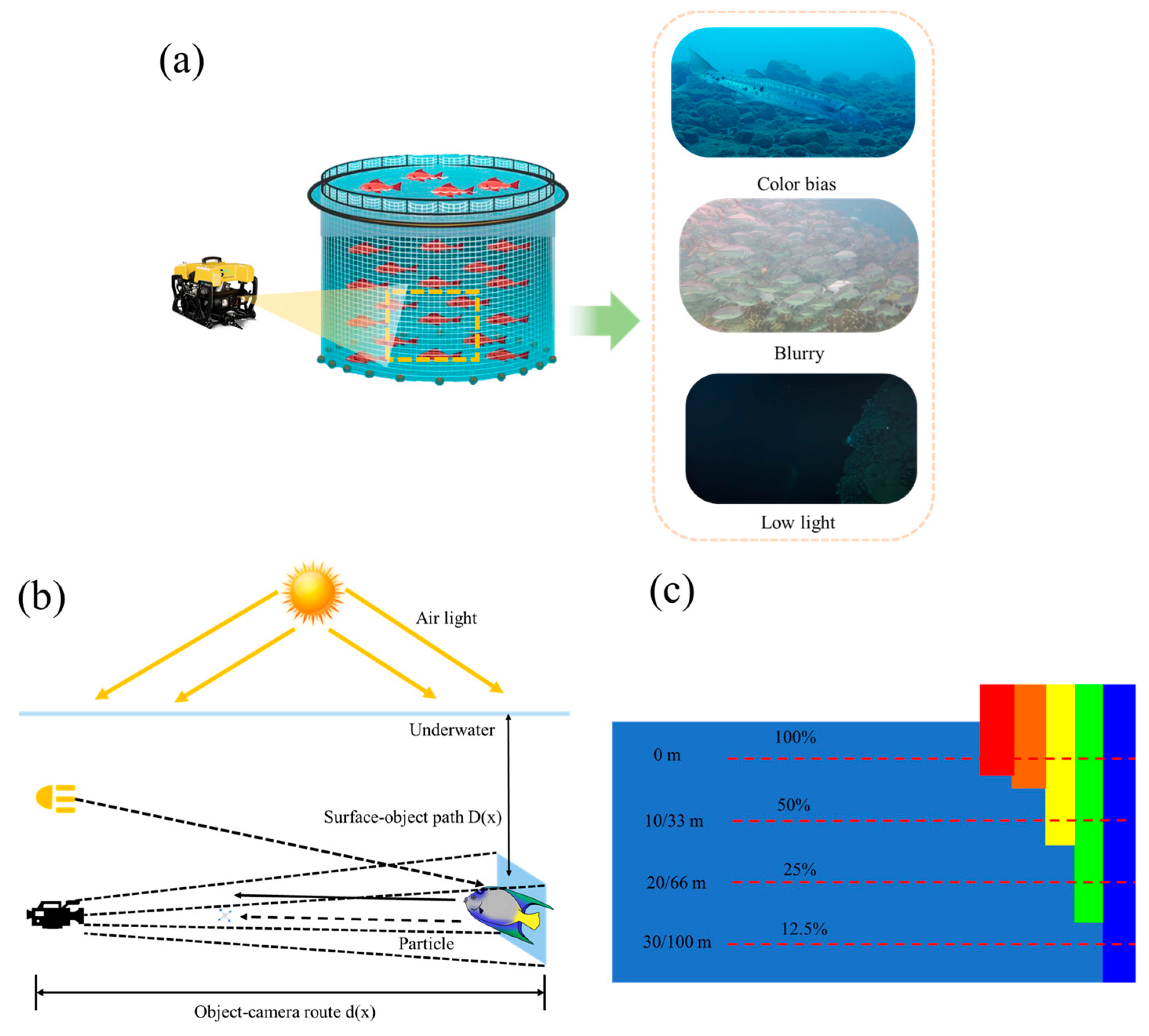
Low-light underwater images often exhibit low global brightness, insufficient contrast, and a loss of local details [
69]. To address these challenges, this paper employs multi-scale histogram equalization as an enhancement technique. This method effectively improves global brightness and contrast while simultaneously enhancing local details [
70,
71].
Multi-scale processing typically uses Gaussian pyramid decomposition or other similar methods to decompose an image into low-frequency components and multiple high-frequency components.
Cumulative distribution function:
Greyscale value
mapped to equalized values:
Multi-scale image fusion:
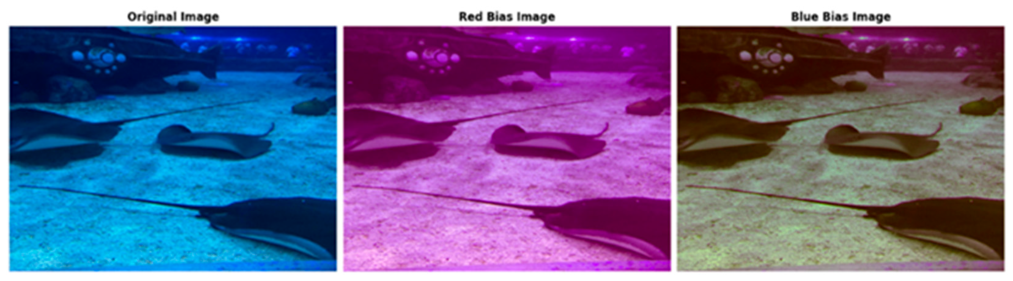
Enhancement methods based on wavelength compensation and contrast correction are well-suited for processing color deviation images [
72,
73]. The wavelength compensation method compensates for each color channel by analyzing the attenuation law of light: restoring the intensity of the red channel and compensating for the long wavelength portion that is absorbed [
74]. Balancing the RGB channel makes the overall color closer to the real scene. Wavelength compensation can effectively correct color bias [
75,
76].
Based on the properties of light attenuation in the water column, the transmittance
is estimated by Eq:
where
is the attenuation coefficient for each channel, reflecting the intensity of water absorption at different wavelengths (red
> green
> blue
).
is the distance from the pixel point to the camera (as appropriate).
In this study, the attenuation coefficients were set to = 0.1, = 0.05, and = 0.03 for the red, green, and blue channels, respectively, based on typical values for clear coastal waters. These reflect the wavelength-dependent attenuation observed in shallow, low-turbidity environments (NTU < 20). The distance was estimated using the dark channel prior method, adapted for underwater images, allowing scene-specific transmission maps. However, these fixed values may not fully represent conditions in deeper or more turbid waters, where attenuation varies significantly.
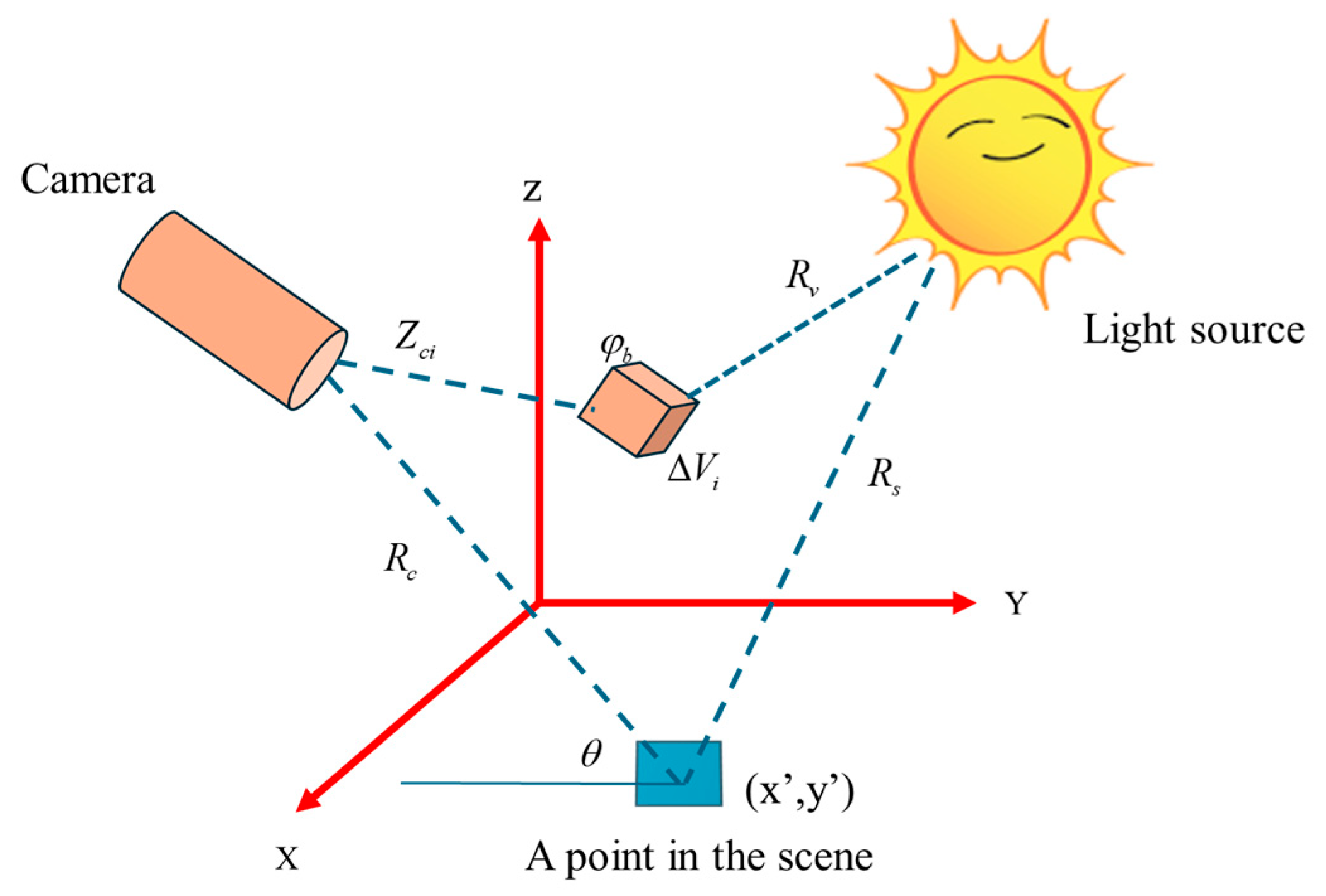
Ambient light
is usually estimated from the pixel area with the highest intensity in the image:
where
is the candidate region in the image, and usually, an area far from the camera is selected as the background.
Based on the simplified model of the underwater image (15), the formula for recovering the real image by backward derivation is as follows:
Based on the absorption properties of water for different wavelengths of light, the attenuation of each channel is compensated for with the following commonly used formula:
is the wavelength compensation factor, usually determined by the absorption properties of water, where is the absorption coefficient for the wavelength c.
Contrast improvement by adjusting pixel intensity distribution is as follows:
where
is the Histogram equalization operation.
The brightness curve is adjusted to improve details in dark areas:
is permanent, 0.4 ≤ x ≤ 0.6.
Enhancement is limited in areas of excessive contrast:
Here, is the parameter used to limit the strength of the histogram equalization.
The combined compensated and corrected image is as follows:
where
is the image enhancement functions (histogram equalization, gamma correction, and other combined operations).
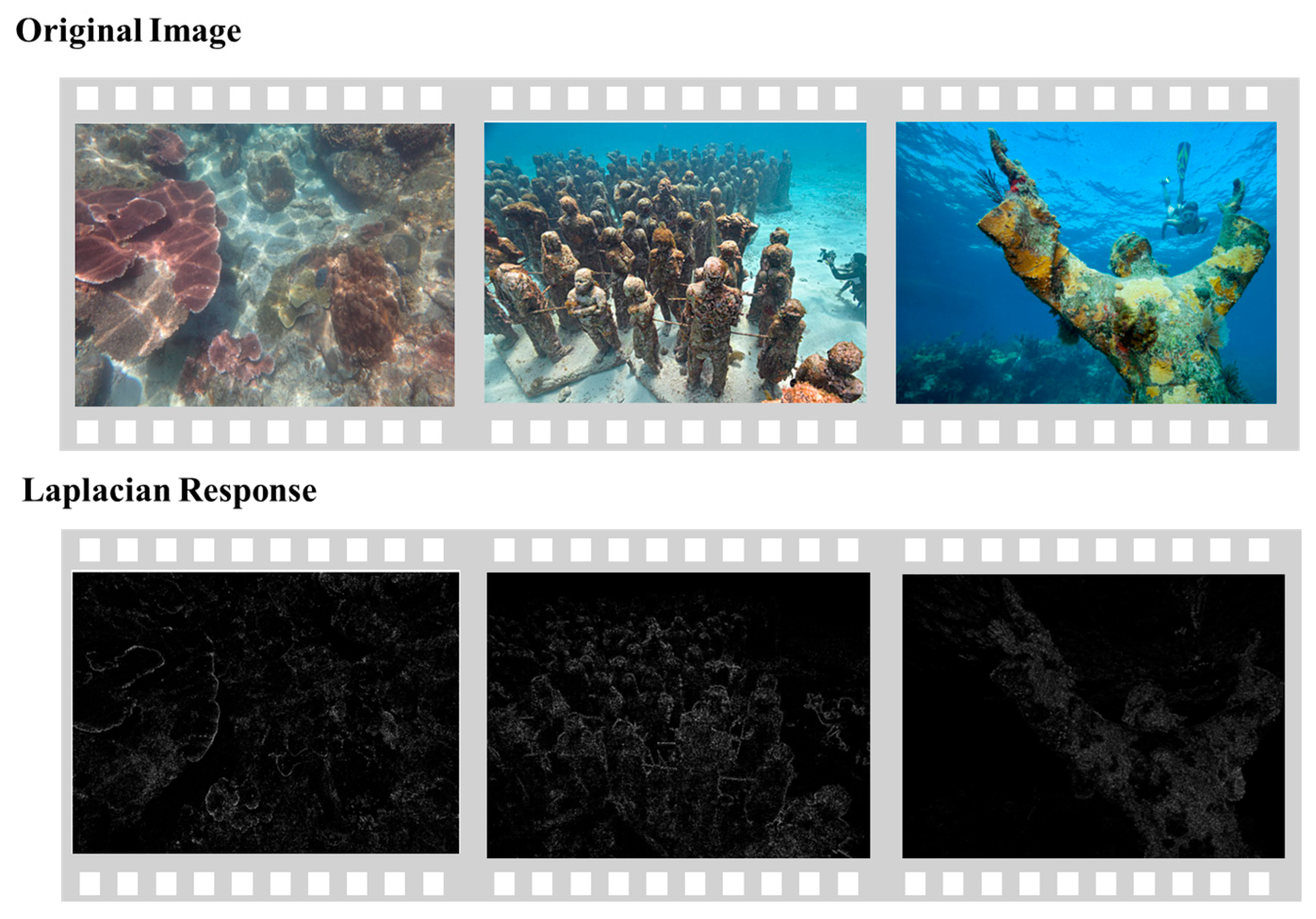
To address the problem of blurred imaging in underwater images, we use a method based on Laplace sharpening.
The fuzzy degradation model can be expressed as follows:
where
is the blurred image.
is the original clear image.
is the point spread function (PSF), which describes the blurring effect.
is the additional noise.
The calculation of the Laplace operator was mentioned earlier (5), which is based on the calculation of high-frequency details by second-order derivatives, which is simplified by changing the variables in it by a different name:
This operator highlights the regions where the brightness of the image changes drastically, i.e., the edge regions. In the discrete case, the convolution is implemented as follows:
The core goal of sharpening is anti-blurring, i.e., the enhancement of the high-frequency component. The optimization formula is as follows:
controls the sharpening intensity, usually in the range of 0.5 ≤ ≤ 1.5.
The parameter
in Equation (36) controls the degree of sharpening applied to the image by scaling the contribution of the Laplacian term,
. In our implementation, we set
= 0.5, a value determined empirically to achieve an optimal balance between enhancing fine details and preventing over-sharpening artifacts, such as ringing or noise amplification. This choice was informed by testing on a variety of images, where
= 0.5 consistently improved sharpness while maintaining image quality, as assessed through visual inspection and quantitative metrics like PSNR, UCIQE, UIQM, RGB, and luminance. The specific image parameters are shown in
Table 1.
For complex scenes, the Laplace operator can also be improved using adjustable edge filters, e.g., high-pass filters:
where
is the scale factor used to control the filter response.
Laplace sharpening amplifies not only edge information but may also enhance noise. The new method proposed in this paper further optimizes the noise suppression.
Combined with Gaussian blurring, a multi-scale image pyramid is constructed:
where
is the scale s of the Gaussian kernel. Based on the multi-scale image pyramid, the high-frequency enhancement part is selected:
where
is the weight of the
s th layer and
is the number of pyramid layers.
Optimized sharpening is based on the traditional Laplace operator, combined with the gradient orientation:
where
, and it indicates the direction of the gradient.
Combined with bilateral filtering, edge-hold noise smoothing is performed before sharpening:
Here, is the normalization factor and controls the degree of the smoothing of intensity similarity. Nonlinear smoothing enhances the accuracy of edge differentiation while reducing noise accumulation after smoothing.
Parameters for Laplace sharpening
can be further designed as an adaptive model:
is the magnitude of the image gradient and is the control parameters that determine the response range.
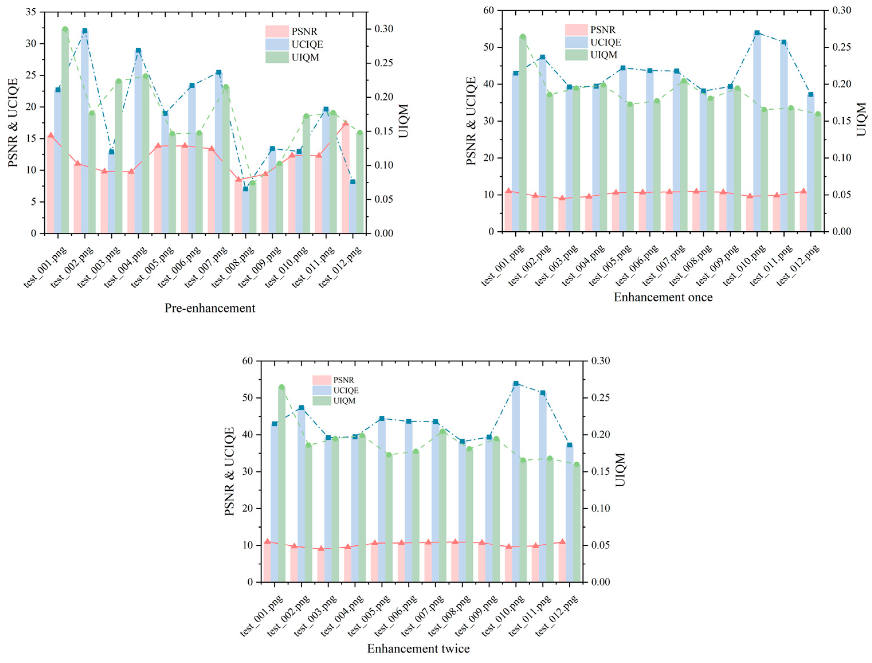
Figure 5 shows the PSNR, UCIQE, and UIQM values of the pictures at the original stage, after one enhancement and after two enhancements.
Figure 5 compares the image quality metrics—peak signal-to-noise ratio (PSNR), Underwater Color Image Quality Evaluation (UCIQE), and underwater image quality measure (UIQM)—for the original underwater image, after one enhancement, and after two enhancements. The PSNR values, ranging from 9 to 11, indicate that the enhancement process maintains low noise levels, though these relatively low scores suggest some residual distortion persists, an area for potential refinement. The UCIQE values, increasing from 37 to 54, reflect significant improvements in color restoration, a critical factor for enhancing the visual clarity of underwater scenes. Meanwhile, the UIQM values, stable between 0.17 and 0.27, demonstrate that the overall quality (encompassing contrast, hue, and sharpness) is preserved without substantial enhancement beyond the first iteration. This stability suggests that our method effectively targets specific distortions—such as color shifts—while maintaining the image’s integrity, a balance essential for applications requiring authentic underwater visuals.
Additionally, it was found that the difference between the results of a single enhancement and two consecutive enhancements was not significant. This suggests that the first enhancement primarily addressed a single type of distortion in the image, and subsequent enhancements did not further improve the quality. In other words, after the first enhancement, the model no longer processed images with normal distortions. This indicates that the enhancement process primarily focused on addressing specific distortions rather than improving the overall image quality in multiple steps.
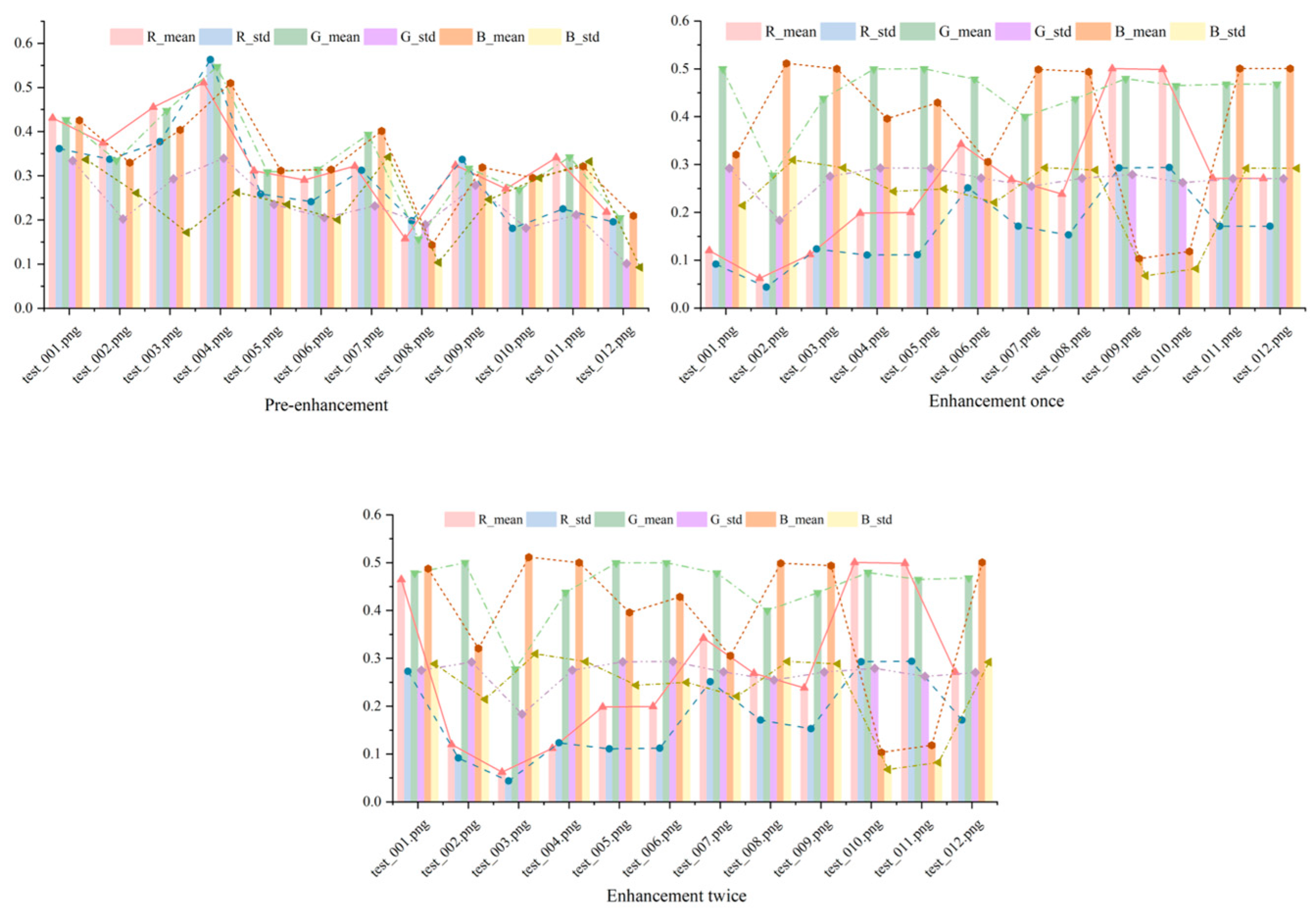
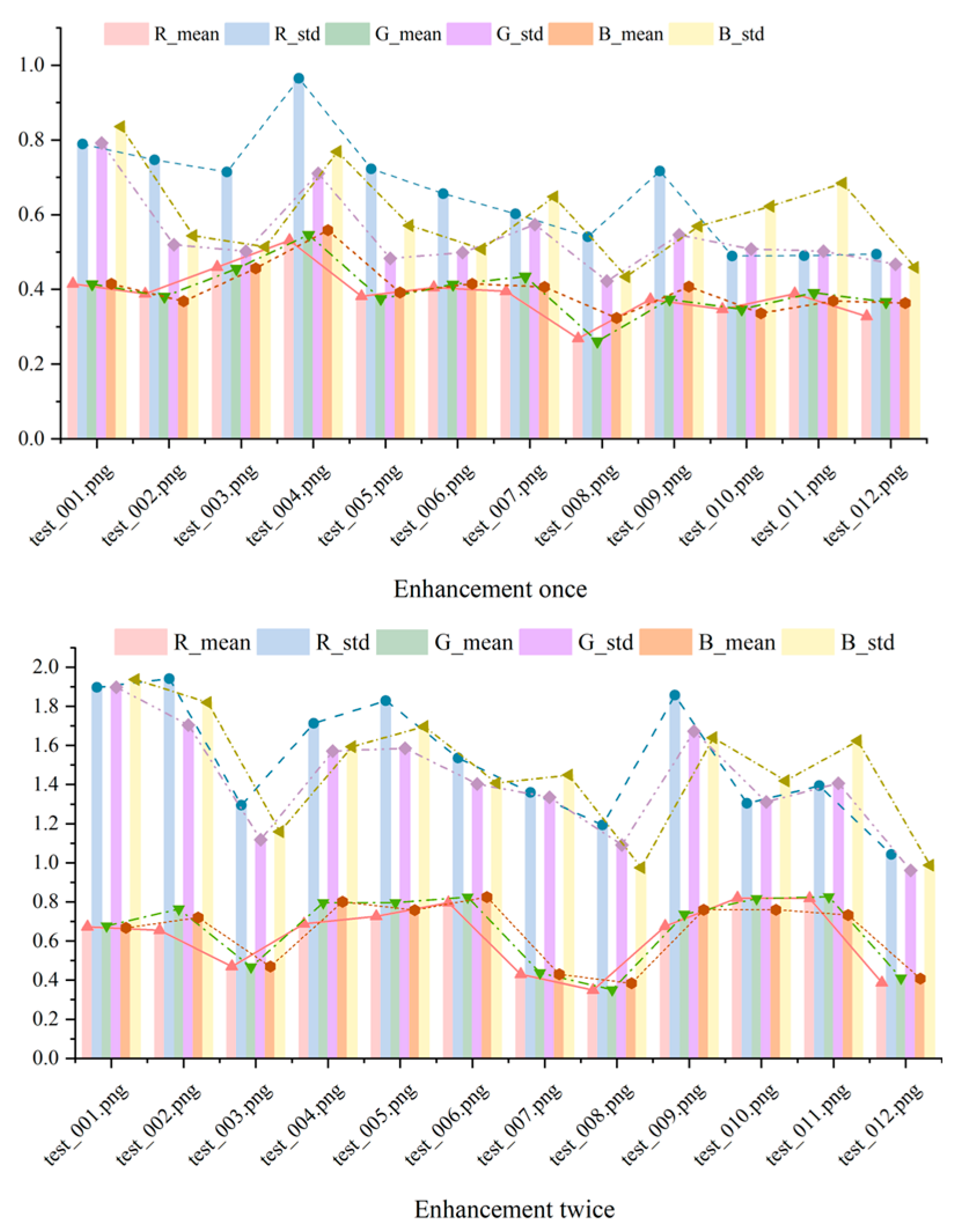
Figure 6 shows the mean and standard deviation of R, G, and B for the original image, the image after one enhancement, and the image after two enhancements.
Figure 6 illustrates the mean and standard deviation of the red (R), green (G), and blue (B) channels across the original image, after one enhancement, and after two enhancements. The mean values shift noticeably after the first enhancement, reflecting a correction in color balance that aligns the image closer to natural underwater hues. However, between the first and second enhancements, these values remain nearly identical, suggesting that the initial enhancement sufficiently mitigates the primary color distortions—likely due to water-induced attenuation. The standard deviations, which are similarly consistent post-first enhancement, indicate that color variability across the image is stabilized, preventing over-processing artifacts.
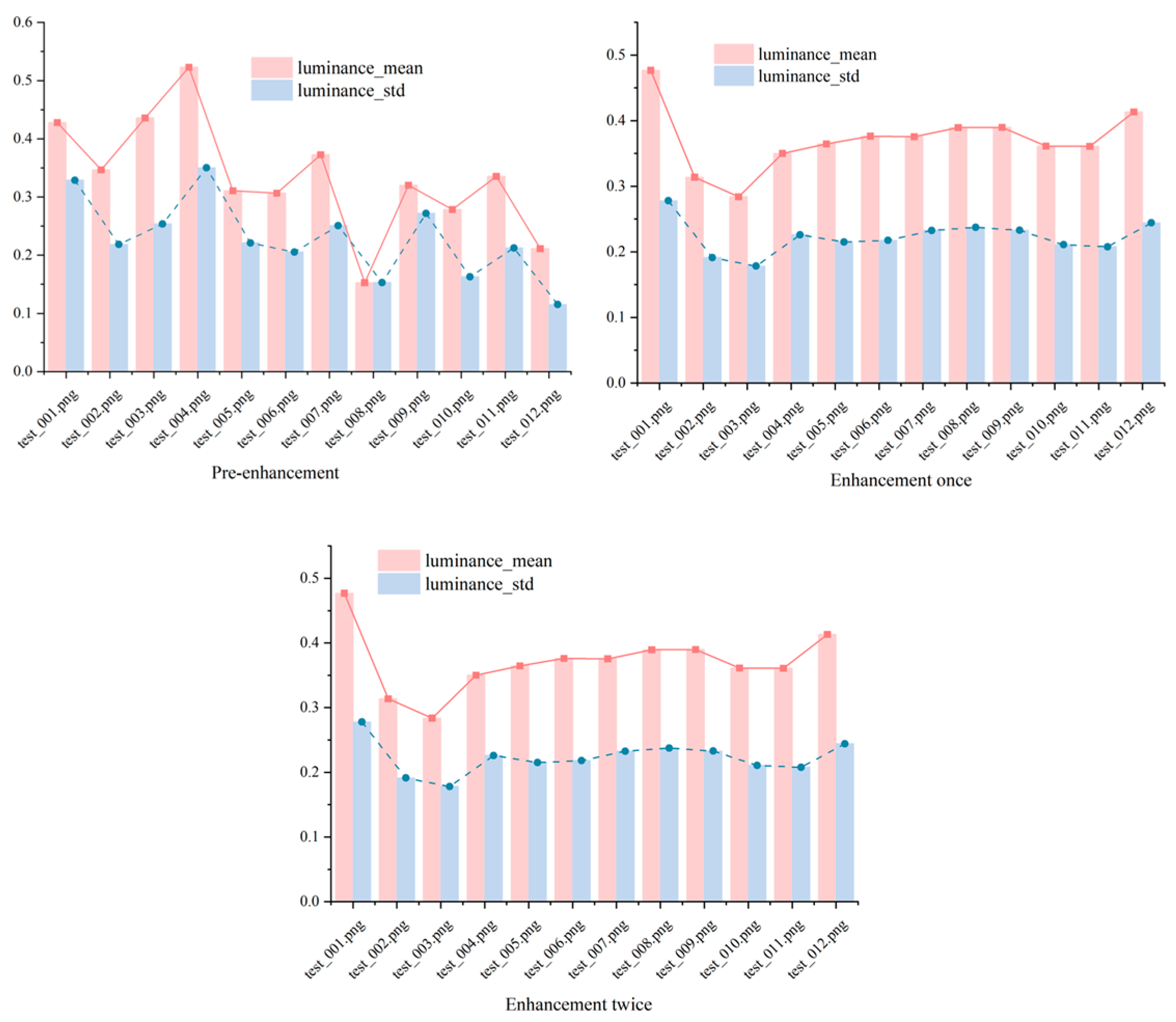
Figure 7 shows the mean and standard deviation of brightness for the original image, after one enhancement, and after two enhancements. The mean brightness rises slightly after the first enhancement, indicating improved illumination that enhances visibility—a vital improvement for underwater environments with poor lighting. However, the lack of significant change between the first and second enhancements suggests that additional processing does not further elevate brightness, preserving the image’s natural appearance. The standard deviation, which remains largely unchanged, reflects consistent brightness uniformity across all stages, implying that our enhancement avoids introducing uneven lighting effects. This outcome is advantageous for maintaining the reliability of underwater images, where uniform brightness aids in accurate object identification and analysis.
Overall, the algorithmic model for underwater image enhancement in special scenarios has a limited effect on improving image quality. While objective quality metrics such as PSNR, UCIQE, and UIQM show small improvements, these changes are insufficient to significantly enhance clarity, color recovery, contrast, and other visual aspects of the image. In particular, there is almost no noticeable difference in terms of color equalization and brightness adjustment between the enhanced image and the original. The model appears to address only a single type of distortion, and the results from the last two enhancements suggest that the first enhancement successfully addresses one specific distortion, while subsequent enhancements do not further improve the image.
These findings underscore the practical utility of our enhancement method in special underwater imaging scenarios. By correcting color distortions and enhancing visibility with minimal noise (as seen in
Figure 5 and
Figure 6) and maintaining brightness uniformity (
Figure 7), our approach enhances image usability for applications like marine biology research, underwater archaeology, and environmental monitoring. The efficiency of achieving substantial improvements in a single enhancement step makes it particularly suitable for real-time systems or resource-constrained settings.
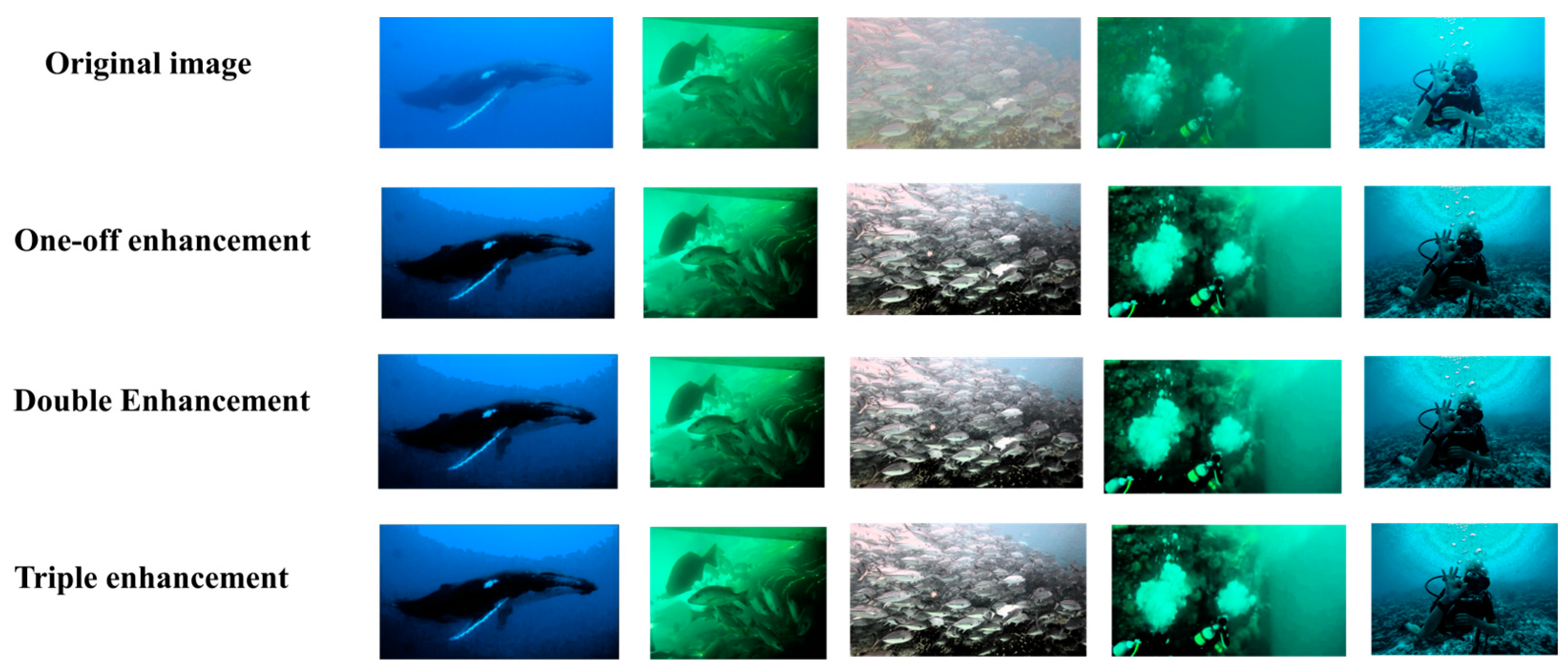
The enhancement results are shown in
Figure 8.
2.3.2. Complex Scenarios Underwater Image Enhancement
Multi-feature fusion techniques are widely employed for underwater image enhancement, particularly in addressing the degradation challenges posed by complex underwater environments [
77,
78,
79]. This advanced image processing approach integrates multiple image features to significantly improve the visual quality and informational clarity of underwater images, making them more suitable for practical applications [
80,
81].
The white balance method is based on the Lambertian reflection model [
82], which corrects the color bias of an image according to the color temperature it presents. For a color image, the color of a point x on the surface of an object in the image can be represented by the Lambertian reflectance model.
Estimation of light source color
:
The mean value of surface reflections from objects with the same attenuation coefficient in an underwater environment is colorless.
Assume that the color of the light source
with an attenuation factor
is a constant:
Bilateral filtering is a nonlinear filtering technique that preserves edge information while smoothing an image [
83,
84]. It combines Gaussian filtering in both spatial and pixel-value domains so that edges are not blurred while smoothing the image [
85]. In our model, we do this by mapping the image to a 3D mesh (a combination of spatial and pixel-valued domains), then applying Gaussian filtering to the mesh, and finally mapping the result back to the original image resolution by interpolation.
Bilateral filter formula:
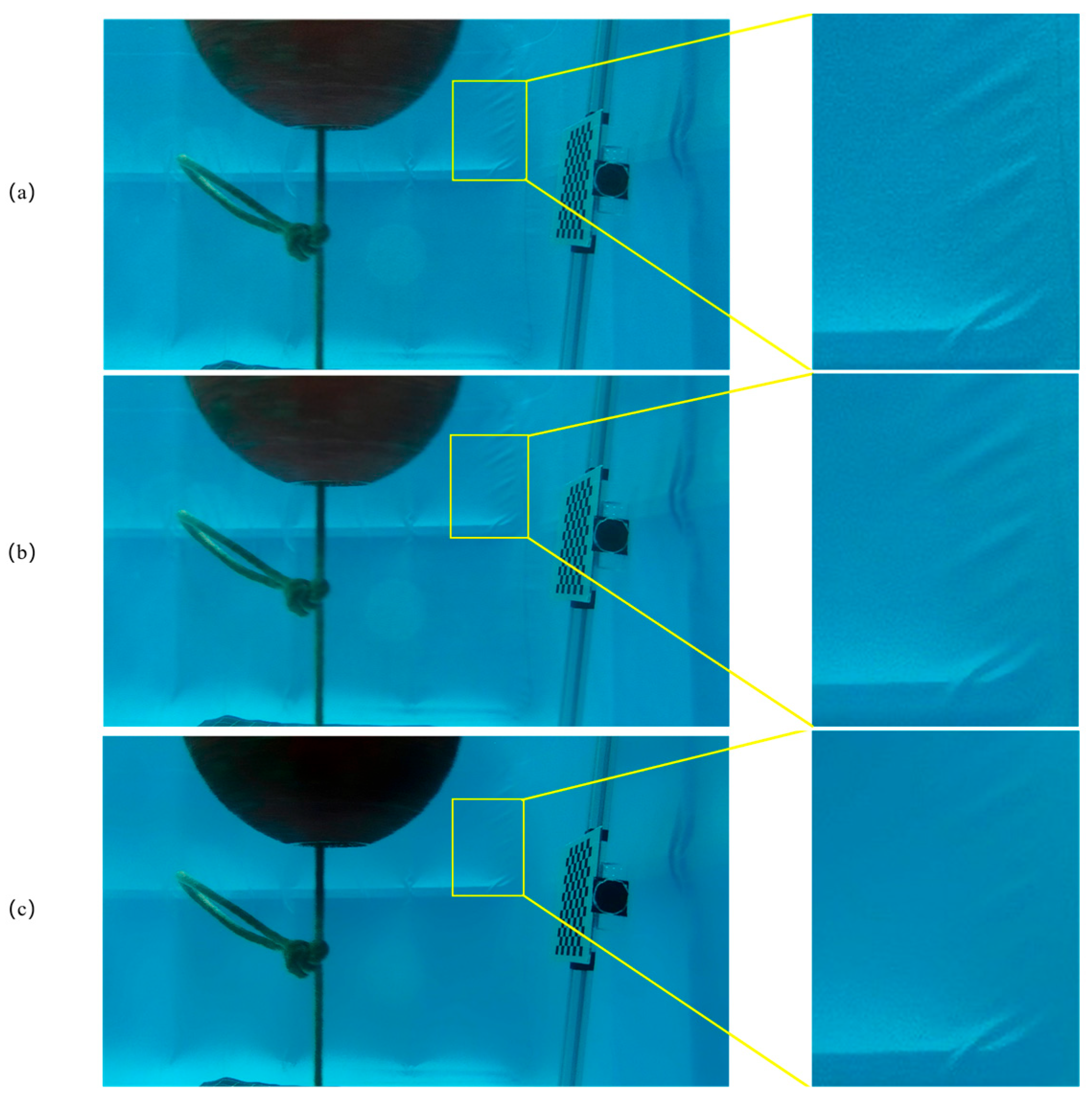
We conducted a comparison of the effect of the filter; if you do not use the parameters of the processing of the function that comes with the openCV, we found that the smoothing effect is more limited after the parameter qualification of the smoothing effect, as shown in
Figure 9c.
Final fused image formula:
Figure 10 presents the PSNR, UCIQE, and UIQM values of the images after one and two enhancements using the fusion enhancement model. The PSNR values indicate that both the first and second enhancements result in some improvement in image quality. The UCIQE shows a significant enhancement after the first application, with the algorithm performing well and achieving natural, consistent color correction. However, after the second enhancement, issues such as oversaturation or color deviations (e.g., an overpowering blue channel) may arise, leading to a decrease in overall color quality. In contrast, the UIQM suggests that a single enhancement is better aligned with typical underwater image enhancement requirements in terms of color quality. The second enhancement, however, increases overall detail.
Figure 11 shows the R, G, and B mean and standard deviation of the image after one enhancement and the image after two enhancements of the enhancement fusion algorithm. The analysis of the mean and standard deviation reveals that the enhancement algorithm significantly impacts the recovery of the color channels. The standard deviation of the red channel is generally higher than that of the green and blue channels, indicating a stronger hue variation during the enhancement process. In contrast, the standard deviation of the green and blue channels is slightly lower, suggesting these channels exhibit less volatility, with the enhancement algorithm having a more stable effect on them. This observation aligns with the light absorption characteristics of water.
Figure 12 illustrates the mean and standard deviation of the image brightness after one and two enhancements using the enhancement fusion method. After the first enhancement, the image brightness is moderate and uniform, with a natural contrast. Following the second enhancement, the average brightness increases, potentially revealing more details with greater clarity.
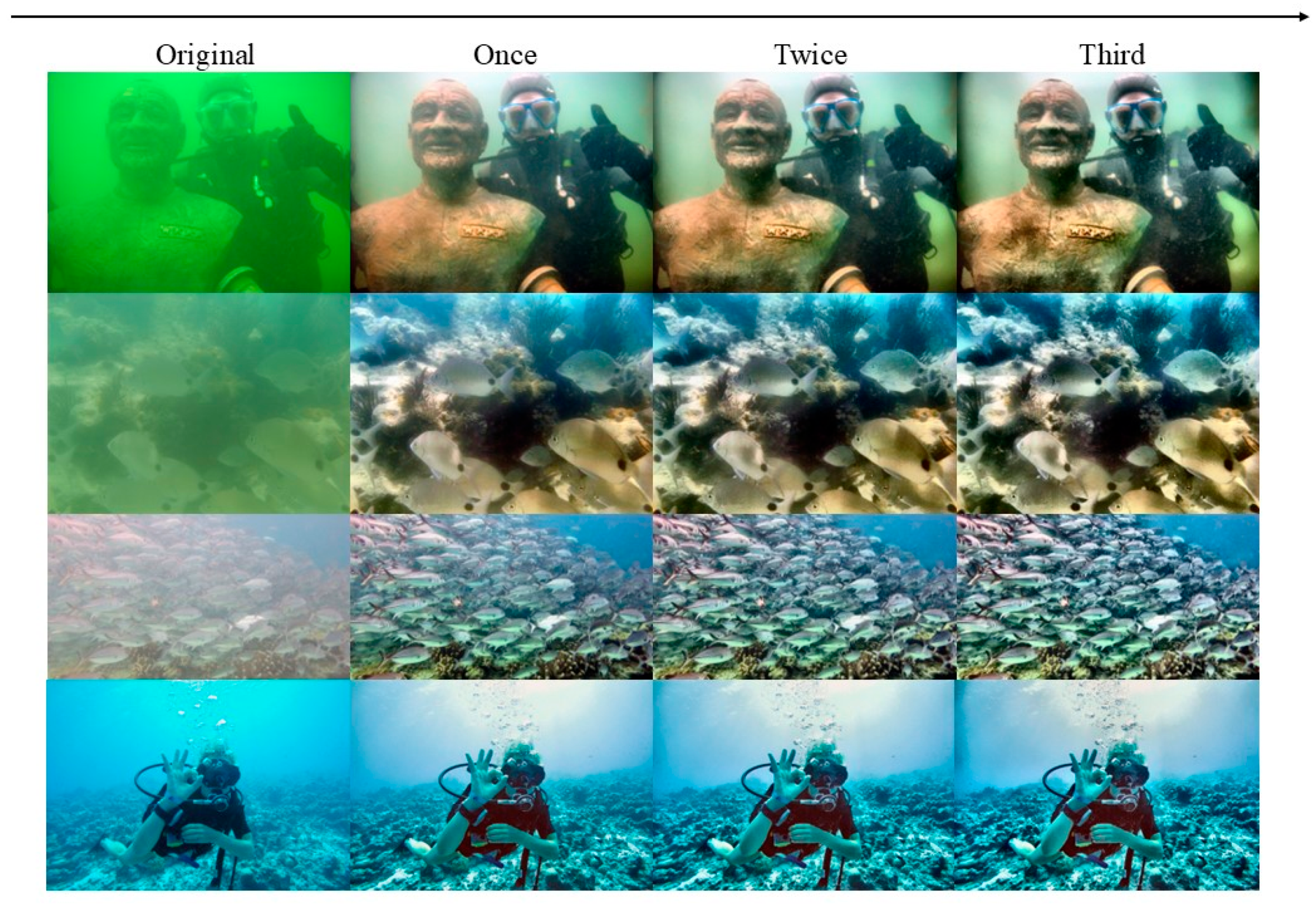
In summary, the underwater image enhancement method proposed in this paper not only offers significant improvements in image quality, noise suppression, and detail retention, but also demonstrates strong adaptability, making it effective for various underwater environments. In shallow-water areas with strong light, the degradation is primarily caused by bluish tones and slight blurring [
86]. In such cases, the enhancement delivers superior performance, with natural color correction and no noticeable distortion. In medium and deep water, where light gradually diminishes, degradation is characterized by a low contrast and a slight increase in noise [
87]. A second enhancement offers some advantages in terms of brightness improvement, but care should be taken to avoid over-enhancement in detailed areas. For deep-water environments, where light is almost nonexistent and degradation is dominated by strong blur and noise, a second enhancement provides a significant improvement in visibility through increased brightness. The enhancement results are shown in
Figure 13.
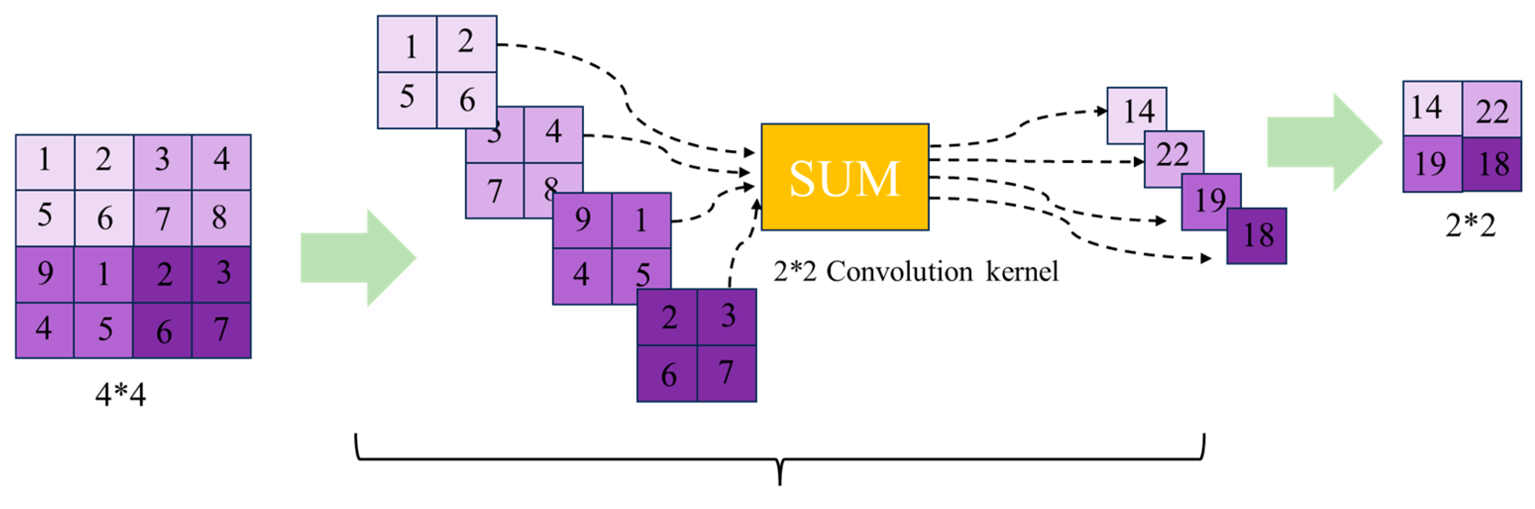
2.3.3. Laplace Pyramid Decomposition
By implementing the aforementioned multi-feature fusion method for image enhancement, it was observed that directly applying the method can introduce negative effects, such as artifacts [
88]. To address these issues, this paper incorporates the Laplacian pyramid method into the process [
89,
90]. This approach is built upon the Gaussian pyramid, which progressively down samples the image, creating a multi-scale representation through resolution reduction. The Laplacian pyramid further enhances this structure by generating layers that capture details between each scale, effectively representing information at different frequency levels within the image.
Similar to the input image, each weight map is processed into a multi-scale version through Gaussian pyramid decomposition. This decomposition smooths the weight maps and mitigates sharp transitions at the boundaries [
91], effectively reducing the risk of introducing artifacts during the fusion process. The input image and the weight map are fused at each layer of the Laplace pyramid and Gaussian pyramid, respectively [
92].
Finally, the fusion results of all layers are reconstructed by progressively combining them from the bottom up to obtain the final enhanced image. This approach ensures that the fused image preserves high-frequency details while maintaining a natural global distribution of brightness and contrast [
93]. Laplace decomposition is shown in
Figure 14.
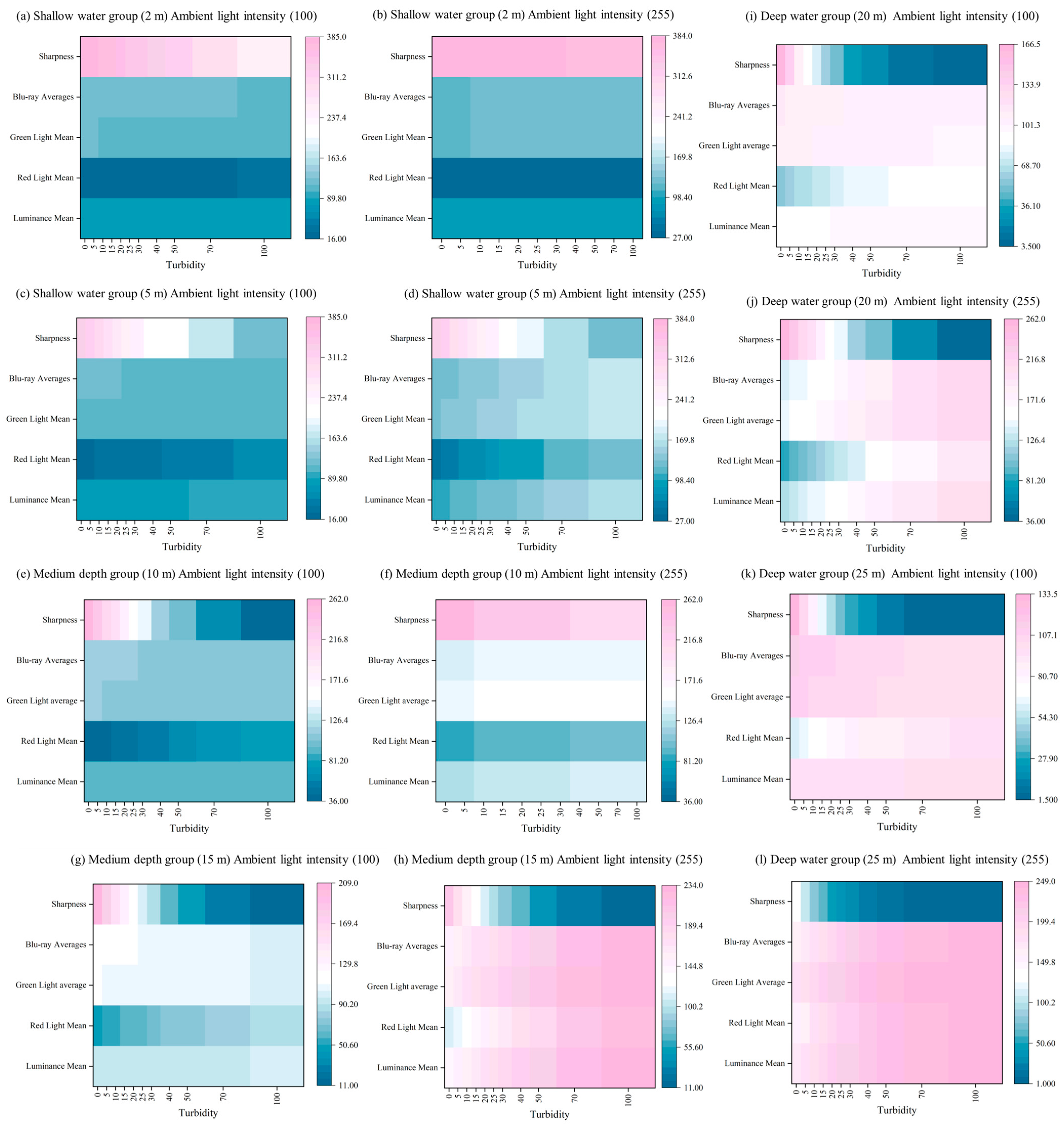
In this subsection, experiments are conducted using the constructed physical model to generate degraded images influenced by three key variables: depth, turbidity, and background light. To simulate various environmental conditions effectively, the experiment was designed with different experimental groups. Water depth was categorized into three classes: the shallow-water group (depths of 2 m and 5 m), the medium-depth group (10 m and 15 m), and the deep-water group (20 m and 25 m). Turbidity levels were set at 0, 5, 10, 15, 20, 25, 30, 40, 50, 70, and 100. Additionally, ambient light conditions were divided into two categories: low light (50) and high light (255).
The experimental results are shown in
Figure 15. Observing the hotspot map reveals a significant decline in image sharpness as depth increases. This phenomenon can be attributed to light attenuation, which reduces the contrast of image details. Additionally, increased turbidity has a pronounced negative impact on sharpness, likely due to the scattering and absorption of light by suspended particles. Within a certain range, enhancing background light intensity improves clarity, though the effect tends to plateau over time.
The mean brightness value decreases progressively with increasing depth and turbidity, indicating overall light attenuation. However, brightness improves with enhanced ambient light. Red light diminishes rapidly with depth, while blue light, characterized by shorter wavelengths, penetrates more effectively underwater. Green light exhibits a pattern of attenuation between that of red and blue light. A strong negative correlation exists between depth and clarity, highlighting depth as the primary factor influencing clarity. Similarly, turbidity shows a strong negative correlation with brightness, reflecting its impact on light scattering intensity. On the other hand, background light demonstrates a strong positive correlation with brightness, suggesting that increasing background light can effectively enhance image brightness. The experimental results are in high agreement with the underwater optical properties, verifying the reasonableness of the degradation model.


