Abstract
Underwater remote sensing image enhancement is complicated by low illumination, color bias, and blurriness, affecting deep-sea monitoring and marine resource development. This study compares a multi-scale fusion-enhanced physical model and deep learning algorithms to optimize intelligent processing. The physical model, based on the Jaffe–McGlamery model, integrates multi-scale histogram equalization, wavelength compensation, and Laplacian sharpening, using cluster analysis to target enhancements. It performs well in shallow, stable waters (turbidity < 20 NTU, depth < 10 m, PSNR = 12.2) but struggles in complex environments (turbidity > 30 NTU). Deep learning models, including water-net, UWCNN, UWCycleGAN, and U-shape Transformer, excel in dynamic conditions, achieving UIQM = 0.24, though requiring GPU support for real-time use. Evaluated on the UIEB dataset (890 images), the physical model suits specific scenarios, while deep learning adapts better to variable underwater settings. These findings offer a theoretical and technical basis for underwater image enhancement and support sustainable marine resource use.
1. Introduction
The oceans are abundant in resources [1,2,3], and with the continuous advancement of science and technology, humanity is increasingly exploring their depths [4,5]. Marine fishery farming, as one of the most important industries in the marine sector, has faced challenges in recent years due to offshore water pollution and other factors [6,7]. As a result, there has been a gradual shift from traditional offshore net cage farming to the exploration and development of deep-sea marine ranching [8,9,10].
Underwater imagery is one of the most important sources of marine information, playing a crucial role in the monitoring and management of deep-sea marine ranches [11,12]. However, the complex marine environment often hampers the acquisition of high-quality underwater images, leading to issues such as color distortion, reduced contrast, uneven illumination, and noise. These challenges arise from the absorption and scattering effects of light as it propagates through water, resulting in images with decreased clarity, contrast, and color fidelity. This directly impacts the accuracy of visual perception and the subsequent extraction and analysis of important information [13,14,15]. Figure 1a shows three underwater degradation images. Figure 1b shows a schematic diagram of the imaging process for an underwater image. Figure 1c shows the absorption behavior of light underwater.

Figure 1.
(a) Three types of underwater degradation images. (b) Schematic diagram of underwater imaging process. (c) Absorption properties of light in water.
Zhou et al. proposed a multi-feature fusion method (MFFM) to enhance underwater images affected by color distortion and low contrast. MFFM combines color correction and contrast enhancement techniques, generating a fusion weight map based on the features of the color-corrected and contrast-enhanced images. This method effectively balances color and contrast while preserving the natural characteristics of the image [16].
Li et al. introduced the Underwater Image Enhancement Benchmark (UIEB), a dataset of 950 real-world underwater images designed to evaluate and advance underwater image enhancement algorithms. They also presented water-net, a convolutional neural network model trained on this dataset to improve image quality. Water-net is a fully convolutional network that integrates inputs with predicted confidence maps. A feature transformation unit optimizes the input before fusion, enhancing the overall results [17].
A new underwater image enhancement method was proposed by Ancuti et al., which introduces a multi-scale fusion technique that combines inputs from white-balanced images. This method applies gamma correction and edge sharpening to improve visibility. By using normalized weight mapping, the technique efficiently blends the inputs to produce artifact-free images [18].
Garg et al. proposed a novel method for enhancing underwater images that combines contrast-limited adaptive histogram equalization (CLAHE) with a percentile approach to improve image clarity and visibility [19].
Yang et al. present a solution for underwater image enhancement using a deep residual framework, which involves generating synthetic training data and employing a VDSR model for super-resolution tasks via CycleGAN. They introduce the underwater reset (uresNet) model, which improves the loss function by incorporating a multinomial approach that includes Edge Difference Loss (EDL) and Mean Error Loss, enhancing image quality [20].
Hou et al. present a large synthetic underwater image dataset (SUID) designed to enhance the evaluation of underwater image enhancement and restoration algorithms. The SUID consists of 900 images generated using the Underwater Image Synthesis Algorithm (UISA), featuring various degradation types and turbidity levels [21].
Zhang et al. present a contrast enhancement method that involves color channel attenuation correction while preserving image details. The approach utilizes a specially designed attenuation matrix to address poor-quality color channels and employs a bi-histogram-based technique for both global and local contrast enhancement [22].
Guo et al. present a novel approach to underwater image enhancement using a multi-scale dense generative adversarial network (MSDB-GAN) that integrates residual learning and dense connectivity techniques. The method employs a multinomial loss function to generate visually appealing enhancement results [23].
Underwater image enhancement methodologies have evolved along two distinct trajectories: physics-based traditional approaches and data-driven deep learning paradigms. While traditional methods (e.g., Jaffe–McGlamery model [24]) provide interpretable solutions grounded in optical propagation principles, their performance often degrades in complex scenarios due to oversimplified assumptions about water turbidity and heterogeneous lighting conditions. Conversely, deep learning techniques demonstrate remarkable adaptability through learned feature representations (e.g., ResNet architectures [25]), yet remain constrained by substantial data requirements [26] and limited physical interpretability [27]. This methodological dichotomy creates critical knowledge gaps in three aspects:
(1) Absence of empirical evidence quantifying performance boundaries between physics-driven and data-driven approaches across marine environments [28];
(2) Underexplored synergies combining physical priors with neural network architectures (e.g., RD-Unet [29] or MetaUE [30]);
(3) Lack of standardized evaluation protocols addressing both full-reference and non-reference metrics (PSNR/UIQM/UCIQE) and operational feasibility (real-time processing) [31,32].
Our comparative analysis reveals the differences under different approaches for underwater imagery by systematically evaluating classical algorithms against four state-of-the-art depth models in 890 images from the UIEB dataset, but also develops a practical guide for selecting enhancement methods based on depth gradient and turbidity levels—a decision support framework urgently needed in marine rangeland monitoring, where equipment limitations and environmental variability coexist.
2. Traditional Methodologies
2.1. Preprocessing Framework for Degradation Characterization
To enhance underwater images, the first step is to effectively classify the images in the dataset. This requires the selection of appropriate recognition and classification methods based on the characteristics of each degradation type [17]. To this end, we performed a preliminary analysis of the dataset. Images categorized as “fuzzy” exhibited blurred object edges, leading to a loss of detail [33]. This made it difficult to recognize complex textures or fine features. These images resemble out-of-focus photographs, with an overall lack of clarity [34]. Low-light images, on the other hand, are characterized by overall dimness and a lack of contrast between highlights and shadows, making the outlines of objects hard to distinguish [35]. Additionally, these images typically contain a high level of noise [36,37]. Color-biased images primarily exhibit a green or blue hue [38,39], resulting in unnatural color contrast [40] and a loss of the original color fidelity [41]. Red and yellow objects, in particular, are heavily affected, appearing either severely distorted or nearly invisible [42].
2.1.1. Grayscale Conversion and Luminance Analysis
Color images contain a vast amount of information, which can complicate computational processes and reduce efficiency [43]. To address this, RGB three-channel images are converted into single-channel grayscale images [44]. There are three common methods for grayscale conversion: the maximum value method, the average value method, and the weighted average method [45,46,47]. In this study, the weighted average method is employed, where the R, G, and B components are averaged based on specific weights [48].
where represents the pixel value of the image after grayscale conversion, while , , and denote the pixel values of the red, green, and blue channels of the original image, respectively.
In digital image processing, Digital Average Brightness (DA) is a metric that quantifies the overall brightness level of an image. It is calculated as the average of pixel values, providing a straightforward measure of the image’s overall luminance.
Here, and represent the height and width of the image, respectively, defining its pixel dimensions. denotes the luminance value at the pixel located at position .
The absolute value of the luminance deviation is defined as the average of the ab-solute values of the pixel luminance values that deviate from the mean value.
where is the average brightness of the image. According to the intermediate value of the grey scale value, takes the value of 128. The larger the value of , the greater the fluctuation in the distribution of luminance values within the image, resulting in a more pronounced contrast between bright and dark areas. Conversely, the smaller the value of , the more uniform the luminance distribution becomes.
The weighted calculation utilizes information about the luminance distribution of the image. The grayscale histogram, Hist[i], represents the frequency of pixels with a luminance value of i in the image, indicating how often each luminance value appears. The range of luminance values in the image spans from 0 to 255.
The luminance anomaly parameter is a parameter that measures the relative relationship between the overall deviation in image luminance and the deviation in luminance distribution.
When the value of is less than 1, it indicates that the overall luminance deviation of the image is small relative to the deviation in the luminance distribution. This means the luminance distribution is more uniform, with no significant luminance anomalies. Conversely, when is greater than 1, it suggests that the overall brightness deviation of the image is larger than the deviation in the brightness distribution. This often results in noticeable brightness abnormalities, such as brightness being concentrated within a certain range or exhibiting significant unevenness.
2.1.2. Laplacian Sharpness Detection
Sharpness degradation, characterized by blurred edges and the loss of fine details, is a common issue in underwater imaging [49]. The Laplacian variance-based method provides a robust quantitative measure for evaluating image sharpness, enabling the targeted enhancement of degraded regions [50].
The Laplacian variance-based method is a classic algorithm for evaluating image sharpness. It assesses sharpness by calculating the Laplacian operator of the image, which highlights the high-frequency components that correspond to image details [51]. The Laplacian response is shown in Figure 2.

Figure 2.
Laplacian response.
The Laplace operator is a second-order derivative operator, which is a scalar form.
is the i-th pixel value of the Laplace operator result. is the total number of pixels. is the mean value of the Laplace operator result. The higher response value of the Laplace operator indicates that there are more high-frequency components in the image with significant edges and details. The pixel values in its output image fluctuate and have high variance. By comparing the variance with the threshold value, it can be judged whether the image is clear or not. In this section, the value of is taken as 12.
2.1.3. LAB Color Space Analysis
We have selected a color deviation detection technique in the LAB color space to identify color-distorted images. This method leverages the separation of luminance and chromatic information in the LAB space, where L represents luminance, A corresponds to the green-to-red chromaticity channel, and B represents the blue-to-yellow chromaticity channel [52,53]. The advantage of using the LAB color space is its close alignment with human visual perception, offering enhanced adaptability to color variations under different lighting conditions [54,55]. Figure 3 illustrates the color shifts.

Figure 3.
Color cast.
The color space conversion from RGB to LAB involves three main steps: RGB → XYZ → LAB. This is because the LAB color space is based on the CIE XYZ color model, with XYZ being one of the standard color spaces used for color representation.
Convert Linear RGB to XYZ: the RGB image is first converted to XYZ color space by the CIE 1931 standard matrix and subsequently, nonlinear mapping is applied to generate LAB components [56].
Convert Linear RGB to LAB:
where , , and represent the values of the three channels in the final LAB color space, respectively. , , and are the calculated values after conversion from RGB to XYZ.
The design of the LAB color space ensures that each channel value directly corresponds to a specific color property. The A and B channel values for each pixel represent the red–green and blue–yellow attributes of that pixel’s color, respectively. This distinction enables the average values of the A and B channels to effectively describe the overall color tendency of an image, indicating shifts towards red–green or blue–yellow tones.
If is large, the image deviates more significantly in the red–green direction. If is large, the image deviates more significantly in the blue–yellow direction.
By analyzing the standardized deviation of the B channel, the breadth or dispersion of the color distribution in the image can be quantitatively described.
Proportion of chromatic aberration:
As in the case of fuzzy recognition, here again, a threshold is required, . In this section, the value of is taken as four.
2.2. Jaffe–McGlamery Model
The Jaffe–McGlamery model is a classical framework commonly applied in underwater imaging and image enhancement [57,58]. To investigate the degradation characteristics of underwater images and validate the accuracy of the degradation model, this paper develops a degradation model based on the underwater optical transmission model introduced by Jaffe and McGlamery.
2.2.1. Core Imaging Principle
The imaging principle of the Jaffe–McGlamery model is shown in Figure 4.

Figure 4.
3D spatial coordinates of the Jaffe–McGlamery model.
The Jaffe–McGlamery model provides a physical foundation for understanding underwater image degradation by simulating light propagation through water. It decomposes the total irradiance received by the camera into three components:
1. Direct component (): light traveling from the object to the camera without scattering.
2. Forward-scattered component (): light deflected by suspended particles but still reaching the sensor.
3. Backscattered component (): ambient light reflected by water particles towards the camera.
The original model expresses the total irradiance as follows:
However, in practical marine ranch monitoring scenarios (depth < 50 m, NTU < 20), forward scattering contributes less than 5% to the total irradiance. We thus adopt a simplified formulation:
where the variables are defined as follows:
- : scene radiance (ideal image without degradation);
- : transmission map (, β: attenuation coefficient);
- : background light intensity, estimated via dark channel prior [59].
This simplification aligns with field observations in aquaculture environments [60], where turbidity variations are moderate. The model’s wavelength-dependent attenuation (Figure 1c) explains the dominance of blue–green hues in deep water.
2.2.2. Simplified Formulation
The complexity of the original Jaffe–McGlamery model arises from its comprehensive consideration of multiple scattering effects and spatially varying parameters. To adapt this model for practical underwater image enhancement in marine ranch monitoring, we propose three key simplifications supported by empirical and theoretical studies:
1. Neglecting Forward Scattering
Existing studies have shown that in close-range imaging scenarios (e.g., typical camera-to-target distances in aquaculture monitoring), where the optical range is short and the suspended sediment concentration is low (NTU < 20), the image blurring effect due to forward scattering tends to be reduced by the model to a minor factor, and is negligible, especially in shallow waters (<30 m).
Jaffe [61], in modeling low turbidity underwater imaging, noted that forward scattering had less than a 2% effect on image signal-to-noise ratios when the turbidity NTU < 15 and the target distance was less than 10 m.
Mobley [62] derived the radiative transfer equation to indicate that in low turbidity waters (NTU < 20), forward scattering as a proportion of the total scattered energy is typically less than 5 percent. This conclusion is supported by the measured data of Twardowski et al. [63], who found that in clear waters with NTU = 10, backward scattering accounted for more than 90 percent of the total scattering, while forward scattering contributed less than 4 percent.
Although experimental data to directly quantify the contribution of forward scattering are still scarce, theoretical derivations, numerical simulations, and model simplifications have shown that the contribution of forward scattering to the total irradiance can be reasonably neglected in typical aquaculture environments with NTU < 20 and water depths of ≤30 m. This assumption can be further verified by controlled experiments (e.g., using collimated light sources and high-precision irradiance sensors). Future research is needed to further validate the applicability of this assumption through controlled experiments (e.g., using collimated light sources with high-precision irradiance sensors) [64].
This simplification reduces computational complexity while maintaining fidelity, as expressed by the following:
2. Spatially Uniform Background Light
Under low turbulence conditions (NTU < 20) and short imaging ranges (<10 m), the spatial heterogeneity of the backscattered light can be ignored without a significant degradation in accuracy. Experimental studies have shown that the homogeneous background assumption reduces computational complexity by 60–70% while maintaining a PSNR loss of less than 3 dB (corresponding to a visual error of ~3–5%) [65].
In turbid (NTU > 50) or deep-water environments (>30 m), spatial fluctuations in backscattered light can be as large as 20–30% due to significant spatial gradients caused by particle stratification and light attenuation, and the homogeneity assumption will lead to model failure. Neglecting these variations may lead to irradiance estimation errors of more than 15% [66,67].
Based on the above theoretical and experimental basis, it is reasonable and efficient to assume that the background light is locally constant, which is particularly suitable for real-time image enhancement tasks in stable underwater environments such as aquaculture.
In order to synthesize the practical situation, we can simplify the calculation of the background light to the following equation:
where is the observed irradiance (image intensity). is the scene radiance. is the attenuation coefficient. d is the depth (or distance to the object). is the spatially uniform background light intensity, which is assumed to be constant in this formulation.
This equation encapsulates the simplification that is constant across the image, avoiding the need to model complex spatial gradients of background light [68].
The simplified transmission map assumes a constant and a globally estimated , which is computationally efficient and suitable for shallow, stable waters (depth < 10 m, NTU < 20). However, this approach may oversimplify light propagation in complex environments, such as deep or turbid waters, where varies spatially due to changes in depth, turbidity, and illumination. Factors like forward scattering and non-uniform background light, neglected here, could further impact accuracy in such scenarios.
2.3. Traditional Methodologies Example
In this section, we will perform enhancement using traditional underwater image enhancement methods; our underwater image enhancement framework uses a multi-stage iterative architecture. Color balance correction is first performed, followed by LAB spatial decomposition to separate luminance and chrominance. Adaptive histogram equalization and bilateral filtering are then applied to suppress noise while preserving edges. Finally, a multi-scale fusion strategy integrates the enhanced features through Laplace pyramid decomposition.
2.3.1. Scene-Specific Underwater Image Enhancement
Low-light underwater images often exhibit low global brightness, insufficient contrast, and a loss of local details [69]. To address these challenges, this paper employs multi-scale histogram equalization as an enhancement technique. This method effectively improves global brightness and contrast while simultaneously enhancing local details [70,71].
Multi-scale processing typically uses Gaussian pyramid decomposition or other similar methods to decompose an image into low-frequency components and multiple high-frequency components.
Cumulative distribution function:
Greyscale value mapped to equalized values:
Weight of details:
Multi-scale image fusion:
Enhancement methods based on wavelength compensation and contrast correction are well-suited for processing color deviation images [72,73]. The wavelength compensation method compensates for each color channel by analyzing the attenuation law of light: restoring the intensity of the red channel and compensating for the long wavelength portion that is absorbed [74]. Balancing the RGB channel makes the overall color closer to the real scene. Wavelength compensation can effectively correct color bias [75,76].
Based on the properties of light attenuation in the water column, the transmittance is estimated by Eq:
where is the attenuation coefficient for each channel, reflecting the intensity of water absorption at different wavelengths (red > green > blue ). is the distance from the pixel point to the camera (as appropriate).
In this study, the attenuation coefficients were set to = 0.1, = 0.05, and = 0.03 for the red, green, and blue channels, respectively, based on typical values for clear coastal waters. These reflect the wavelength-dependent attenuation observed in shallow, low-turbidity environments (NTU < 20). The distance was estimated using the dark channel prior method, adapted for underwater images, allowing scene-specific transmission maps. However, these fixed values may not fully represent conditions in deeper or more turbid waters, where attenuation varies significantly.
Ambient light is usually estimated from the pixel area with the highest intensity in the image:
where is the candidate region in the image, and usually, an area far from the camera is selected as the background.
Based on the simplified model of the underwater image (15), the formula for recovering the real image by backward derivation is as follows:
Based on the absorption properties of water for different wavelengths of light, the attenuation of each channel is compensated for with the following commonly used formula:
is the wavelength compensation factor, usually determined by the absorption properties of water, where is the absorption coefficient for the wavelength c.
Contrast improvement by adjusting pixel intensity distribution is as follows:
where is the Histogram equalization operation.
The brightness curve is adjusted to improve details in dark areas:
is permanent, 0.4 ≤ x ≤ 0.6.
Enhancement is limited in areas of excessive contrast:
Here, is the parameter used to limit the strength of the histogram equalization.
The combined compensated and corrected image is as follows:
where is the image enhancement functions (histogram equalization, gamma correction, and other combined operations).
To address the problem of blurred imaging in underwater images, we use a method based on Laplace sharpening.
The fuzzy degradation model can be expressed as follows:
where is the blurred image. is the original clear image. is the point spread function (PSF), which describes the blurring effect. is the additional noise.
The calculation of the Laplace operator was mentioned earlier (5), which is based on the calculation of high-frequency details by second-order derivatives, which is simplified by changing the variables in it by a different name:
This operator highlights the regions where the brightness of the image changes drastically, i.e., the edge regions. In the discrete case, the convolution is implemented as follows:
The core goal of sharpening is anti-blurring, i.e., the enhancement of the high-frequency component. The optimization formula is as follows:
controls the sharpening intensity, usually in the range of 0.5 ≤ ≤ 1.5.
The parameter in Equation (36) controls the degree of sharpening applied to the image by scaling the contribution of the Laplacian term, . In our implementation, we set = 0.5, a value determined empirically to achieve an optimal balance between enhancing fine details and preventing over-sharpening artifacts, such as ringing or noise amplification. This choice was informed by testing on a variety of images, where = 0.5 consistently improved sharpness while maintaining image quality, as assessed through visual inspection and quantitative metrics like PSNR, UCIQE, UIQM, RGB, and luminance. The specific image parameters are shown in Table 1.

Table 1.
Picture metrics under different λ conditions.
For complex scenes, the Laplace operator can also be improved using adjustable edge filters, e.g., high-pass filters:
where is the scale factor used to control the filter response.
Laplace sharpening amplifies not only edge information but may also enhance noise. The new method proposed in this paper further optimizes the noise suppression.
Combined with Gaussian blurring, a multi-scale image pyramid is constructed:
where is the scale s of the Gaussian kernel. Based on the multi-scale image pyramid, the high-frequency enhancement part is selected:
where is the weight of the s th layer and is the number of pyramid layers.
Optimized sharpening is based on the traditional Laplace operator, combined with the gradient orientation:
where , and it indicates the direction of the gradient.
Combined with bilateral filtering, edge-hold noise smoothing is performed before sharpening:
Here, is the normalization factor and controls the degree of the smoothing of intensity similarity. Nonlinear smoothing enhances the accuracy of edge differentiation while reducing noise accumulation after smoothing.
Parameters for Laplace sharpening can be further designed as an adaptive model:
is the magnitude of the image gradient and is the control parameters that determine the response range.
Figure 5 shows the PSNR, UCIQE, and UIQM values of the pictures at the original stage, after one enhancement and after two enhancements.
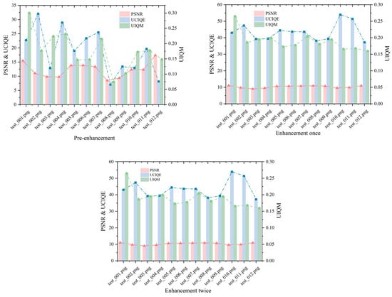
Figure 5.
PSNR, UCIQE, and UIQM values for the original image, the image after one enhancement and the image after two enhancements in specific scenarios.
Figure 5 compares the image quality metrics—peak signal-to-noise ratio (PSNR), Underwater Color Image Quality Evaluation (UCIQE), and underwater image quality measure (UIQM)—for the original underwater image, after one enhancement, and after two enhancements. The PSNR values, ranging from 9 to 11, indicate that the enhancement process maintains low noise levels, though these relatively low scores suggest some residual distortion persists, an area for potential refinement. The UCIQE values, increasing from 37 to 54, reflect significant improvements in color restoration, a critical factor for enhancing the visual clarity of underwater scenes. Meanwhile, the UIQM values, stable between 0.17 and 0.27, demonstrate that the overall quality (encompassing contrast, hue, and sharpness) is preserved without substantial enhancement beyond the first iteration. This stability suggests that our method effectively targets specific distortions—such as color shifts—while maintaining the image’s integrity, a balance essential for applications requiring authentic underwater visuals.
Additionally, it was found that the difference between the results of a single enhancement and two consecutive enhancements was not significant. This suggests that the first enhancement primarily addressed a single type of distortion in the image, and subsequent enhancements did not further improve the quality. In other words, after the first enhancement, the model no longer processed images with normal distortions. This indicates that the enhancement process primarily focused on addressing specific distortions rather than improving the overall image quality in multiple steps.
Figure 6 shows the mean and standard deviation of R, G, and B for the original image, the image after one enhancement, and the image after two enhancements.
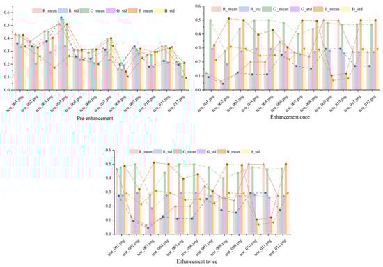
Figure 6.
The mean and standard deviation of R, G, and B for the original image, the image after one enhancement, and the image after two enhancements in specific scenarios.
Figure 6 illustrates the mean and standard deviation of the red (R), green (G), and blue (B) channels across the original image, after one enhancement, and after two enhancements. The mean values shift noticeably after the first enhancement, reflecting a correction in color balance that aligns the image closer to natural underwater hues. However, between the first and second enhancements, these values remain nearly identical, suggesting that the initial enhancement sufficiently mitigates the primary color distortions—likely due to water-induced attenuation. The standard deviations, which are similarly consistent post-first enhancement, indicate that color variability across the image is stabilized, preventing over-processing artifacts.
Figure 7 shows the mean and standard deviation of brightness for the original image, after one enhancement, and after two enhancements. The mean brightness rises slightly after the first enhancement, indicating improved illumination that enhances visibility—a vital improvement for underwater environments with poor lighting. However, the lack of significant change between the first and second enhancements suggests that additional processing does not further elevate brightness, preserving the image’s natural appearance. The standard deviation, which remains largely unchanged, reflects consistent brightness uniformity across all stages, implying that our enhancement avoids introducing uneven lighting effects. This outcome is advantageous for maintaining the reliability of underwater images, where uniform brightness aids in accurate object identification and analysis.

Figure 7.
The mean and standard deviation of the brightness for the original image, the image after one enhancement, and the image after two enhancements in specific scenarios.
Overall, the algorithmic model for underwater image enhancement in special scenarios has a limited effect on improving image quality. While objective quality metrics such as PSNR, UCIQE, and UIQM show small improvements, these changes are insufficient to significantly enhance clarity, color recovery, contrast, and other visual aspects of the image. In particular, there is almost no noticeable difference in terms of color equalization and brightness adjustment between the enhanced image and the original. The model appears to address only a single type of distortion, and the results from the last two enhancements suggest that the first enhancement successfully addresses one specific distortion, while subsequent enhancements do not further improve the image.
These findings underscore the practical utility of our enhancement method in special underwater imaging scenarios. By correcting color distortions and enhancing visibility with minimal noise (as seen in Figure 5 and Figure 6) and maintaining brightness uniformity (Figure 7), our approach enhances image usability for applications like marine biology research, underwater archaeology, and environmental monitoring. The efficiency of achieving substantial improvements in a single enhancement step makes it particularly suitable for real-time systems or resource-constrained settings.
The enhancement results are shown in Figure 8.

Figure 8.
Enhancement results of underwater image models for specific scenarios.
2.3.2. Complex Scenarios Underwater Image Enhancement
Multi-feature fusion techniques are widely employed for underwater image enhancement, particularly in addressing the degradation challenges posed by complex underwater environments [77,78,79]. This advanced image processing approach integrates multiple image features to significantly improve the visual quality and informational clarity of underwater images, making them more suitable for practical applications [80,81].
The white balance method is based on the Lambertian reflection model [82], which corrects the color bias of an image according to the color temperature it presents. For a color image, the color of a point x on the surface of an object in the image can be represented by the Lambertian reflectance model.
Estimation of light source color :
The mean value of surface reflections from objects with the same attenuation coefficient in an underwater environment is colorless.
Assume that the color of the light source with an attenuation factor is a constant:
Bilateral filtering is a nonlinear filtering technique that preserves edge information while smoothing an image [83,84]. It combines Gaussian filtering in both spatial and pixel-value domains so that edges are not blurred while smoothing the image [85]. In our model, we do this by mapping the image to a 3D mesh (a combination of spatial and pixel-valued domains), then applying Gaussian filtering to the mesh, and finally mapping the result back to the original image resolution by interpolation.
Gaussian Spatial Kernel:
Gaussian Range Kernel:
Bilateral filter formula:
We conducted a comparison of the effect of the filter; if you do not use the parameters of the processing of the function that comes with the openCV, we found that the smoothing effect is more limited after the parameter qualification of the smoothing effect, as shown in Figure 9c.

Figure 9.
(a) Original image: the input image without any processing. (b) OpenCV bilateral filter result: the image after processing with cv2.bilateralFilter. (c) Custom bilateral filtering result: the effect of our filter function.
Laplacian Contrast:
Local Contrast:
Saliency:
Exposure:
Final fused image formula:
Figure 10 presents the PSNR, UCIQE, and UIQM values of the images after one and two enhancements using the fusion enhancement model. The PSNR values indicate that both the first and second enhancements result in some improvement in image quality. The UCIQE shows a significant enhancement after the first application, with the algorithm performing well and achieving natural, consistent color correction. However, after the second enhancement, issues such as oversaturation or color deviations (e.g., an overpowering blue channel) may arise, leading to a decrease in overall color quality. In contrast, the UIQM suggests that a single enhancement is better aligned with typical underwater image enhancement requirements in terms of color quality. The second enhancement, however, increases overall detail.
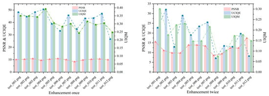
Figure 10.
PSNR, UCIQE, and UIQM values for the original image, the image after one enhancement, and the image after two enhancements in complex scenarios.
Figure 11 shows the R, G, and B mean and standard deviation of the image after one enhancement and the image after two enhancements of the enhancement fusion algorithm. The analysis of the mean and standard deviation reveals that the enhancement algorithm significantly impacts the recovery of the color channels. The standard deviation of the red channel is generally higher than that of the green and blue channels, indicating a stronger hue variation during the enhancement process. In contrast, the standard deviation of the green and blue channels is slightly lower, suggesting these channels exhibit less volatility, with the enhancement algorithm having a more stable effect on them. This observation aligns with the light absorption characteristics of water.
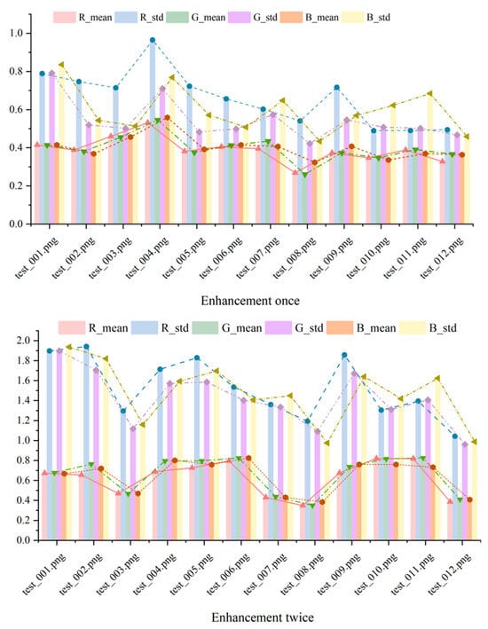
Figure 11.
The mean and standard deviation of R, G, and B for the original image, the image after one enhancement, and the image after two enhancements in complex scenarios.
Figure 12 illustrates the mean and standard deviation of the image brightness after one and two enhancements using the enhancement fusion method. After the first enhancement, the image brightness is moderate and uniform, with a natural contrast. Following the second enhancement, the average brightness increases, potentially revealing more details with greater clarity.

Figure 12.
The mean and standard deviation of the brightness for the original image, the image after one enhancement, and the image after two enhancements in complex scenarios.
In summary, the underwater image enhancement method proposed in this paper not only offers significant improvements in image quality, noise suppression, and detail retention, but also demonstrates strong adaptability, making it effective for various underwater environments. In shallow-water areas with strong light, the degradation is primarily caused by bluish tones and slight blurring [86]. In such cases, the enhancement delivers superior performance, with natural color correction and no noticeable distortion. In medium and deep water, where light gradually diminishes, degradation is characterized by a low contrast and a slight increase in noise [87]. A second enhancement offers some advantages in terms of brightness improvement, but care should be taken to avoid over-enhancement in detailed areas. For deep-water environments, where light is almost nonexistent and degradation is dominated by strong blur and noise, a second enhancement provides a significant improvement in visibility through increased brightness. The enhancement results are shown in Figure 13.

Figure 13.
Enhancement results of underwater image model under enhanced fusion model.
2.3.3. Laplace Pyramid Decomposition
By implementing the aforementioned multi-feature fusion method for image enhancement, it was observed that directly applying the method can introduce negative effects, such as artifacts [88]. To address these issues, this paper incorporates the Laplacian pyramid method into the process [89,90]. This approach is built upon the Gaussian pyramid, which progressively down samples the image, creating a multi-scale representation through resolution reduction. The Laplacian pyramid further enhances this structure by generating layers that capture details between each scale, effectively representing information at different frequency levels within the image.
Similar to the input image, each weight map is processed into a multi-scale version through Gaussian pyramid decomposition. This decomposition smooths the weight maps and mitigates sharp transitions at the boundaries [91], effectively reducing the risk of introducing artifacts during the fusion process. The input image and the weight map are fused at each layer of the Laplace pyramid and Gaussian pyramid, respectively [92].
Finally, the fusion results of all layers are reconstructed by progressively combining them from the bottom up to obtain the final enhanced image. This approach ensures that the fused image preserves high-frequency details while maintaining a natural global distribution of brightness and contrast [93]. Laplace decomposition is shown in Figure 14.
Figure 14.
Laplace decomposition.
In this subsection, experiments are conducted using the constructed physical model to generate degraded images influenced by three key variables: depth, turbidity, and background light. To simulate various environmental conditions effectively, the experiment was designed with different experimental groups. Water depth was categorized into three classes: the shallow-water group (depths of 2 m and 5 m), the medium-depth group (10 m and 15 m), and the deep-water group (20 m and 25 m). Turbidity levels were set at 0, 5, 10, 15, 20, 25, 30, 40, 50, 70, and 100. Additionally, ambient light conditions were divided into two categories: low light (50) and high light (255).
The experimental results are shown in Figure 15. Observing the hotspot map reveals a significant decline in image sharpness as depth increases. This phenomenon can be attributed to light attenuation, which reduces the contrast of image details. Additionally, increased turbidity has a pronounced negative impact on sharpness, likely due to the scattering and absorption of light by suspended particles. Within a certain range, enhancing background light intensity improves clarity, though the effect tends to plateau over time.
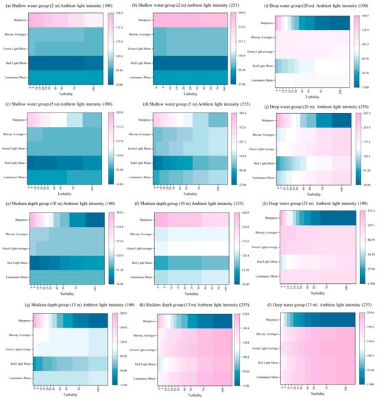
Figure 15.
Results of the experiment.
The mean brightness value decreases progressively with increasing depth and turbidity, indicating overall light attenuation. However, brightness improves with enhanced ambient light. Red light diminishes rapidly with depth, while blue light, characterized by shorter wavelengths, penetrates more effectively underwater. Green light exhibits a pattern of attenuation between that of red and blue light. A strong negative correlation exists between depth and clarity, highlighting depth as the primary factor influencing clarity. Similarly, turbidity shows a strong negative correlation with brightness, reflecting its impact on light scattering intensity. On the other hand, background light demonstrates a strong positive correlation with brightness, suggesting that increasing background light can effectively enhance image brightness. The experimental results are in high agreement with the underwater optical properties, verifying the reasonableness of the degradation model.
3. Cluster Analysis
This study adopts a bibliometric methodology to investigate the historical progression of underwater image enhancement. Data for the analysis, including journals, research fields, national contributions, and institutional involvements, were systematically extracted from the Web of Science (WOS) database. Recognized as a leading citation index resource, WOS provides access to nearly 100 years of multidisciplinary scholarly works, representing foundational research across diverse domains. The database is distinguished by its inclusion of high-impact journals, making it an indispensable tool for researchers seeking credible academic references. Its prominence and reliability within the scholarly community are further corroborated by its authoritative standing.
The following are the key logical formulae that we used for the search: TS = (“underwater”) and TS = (“image*” OR “picture*”) and TS = (“enhancement” OR “restoration” OR “processing” OR “intensification”). The initial default screening searched all years on Web of Science, and approximately 2332 pieces of the relevant literature were screened. The earliest documentation in WOS dates back to 2002; we searched all years for articles published in English. For the article type, we chose “Article”. In the end, we retrieved 2244 articles from Web of Science after deduplication using “CiteSpace”. After manual screening, we selected 2057 references as a sample for the bibliometric data analysis. The specific search process is shown in Figure 16.

Figure 16.
Schematic diagram of the search process.
The referenced papers were selected based on their relevance to underwater image enhancement, prioritizing peer-reviewed publications that address traditional physics-based methods and deep learning approaches. Seminal works laying the methodological foundation (e.g., Ref. [24]) and recent studies introducing novel techniques or datasets (e.g., Ref. [17]) were included to ensure a comprehensive and credible review. The selection also aimed to cover diverse methodologies—such as CNNs, GANs, and Transformers—to contextualize our comparative analysis.
3.1. Country Analysis
In the CiteSpace user interface, time slicing selects January 2002 to December 2025, time slicing is per year, node types selects country, and selection criteria selects the g-index, k = 25. Pruning selects Pathfinder and prunes the merged network; a picture of the finished process is shown in Figure 17.

Figure 17.
Country cluster analysis based on CiteSpace.
Figure 17 shows that as many as 74 countries and regions have published papers related to underwater image enhancement. We can see that almost the whole world is focusing on the field of underwater image enhancement and contributing to the marine field as much as possible. The size of each node represents the number of posts. Among them, China, the United States, India, and Australia are extremely prominent in contributing to the field of underwater image enhancement.
The color of the node represents the year; the closer the color is to red, the closer the publication time is to the present. As can be seen in Figure 17, the node for China changes from purple to red, which means that China’s image enhancement research started earlier. The larger nodes in the figure are colored red, indicating that underwater image enhancement is a focus that these countries are paying close attention to.
China dominates the number of publications in this area, with a count of 1361, which is almost two-thirds of the total number of publications, followed by the United States, with a count of 162 (7.88%), India, with a count of 133 (6.47%), and Australia, with a count of 83 (4.04%) (Table 2).
Table 2.
Top 10 underwater image enhancement posts.
We visualized the country data we had on a world map and the results obtained are shown in Figure 18.
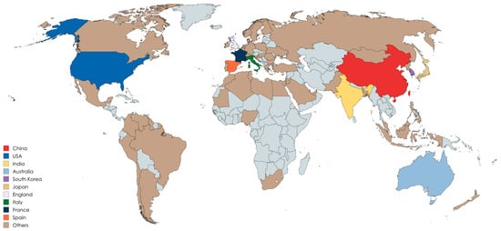
Figure 18.
Distribution of countries and regions with published papers.
As shown in Figure 18, most of the regions involved in underwater image enhancement are coastal countries, which have an inherent geographic location. The top ten countries in terms of the number of publications are all coastal regions, which have greater technological needs in this area than inland regions.
We have made a chord diagram of the cooperation between countries, as shown in Figure 19.
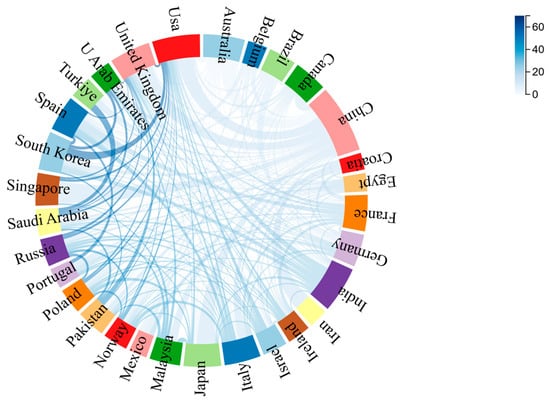
Figure 19.
Chord charts of cooperation relations among countries.
In Figure 19 and the chord diagram, the length of the colored band represents the number of articles issued by the country; because China issued a large number of articles, we have taken the logarithmic operation of the value. The relationship of the connecting line represents the cooperation, and the depth of the connecting line represents the amount of cooperation. In the figure, we find that the countries with a medium level of publications are closely related to each other, for example, USA and South Korea and Turkey and Saudi Arabia have darker-colored ties; on the contrary, China, which is the country with the highest number of publications, has less cooperation with other countries, with lighter-colored ties and a smaller number of ties.
3.2. Institution Analysis
In this section, we present the institutional analysis. Figure 20 is the clustering image we made using “VOSviewer”; again, the node size represents the number of postings and the connecting line represents the partnership. From the figure, we can see that the highest number of postings is Dalian Maritime University with 120 postings, followed closely by Chinese Academy of Sciences with 116 articles, followed by Harbin Engineering University with 84 articles. Table 3 shows the ranking of the top 15 institutions in terms of the number of articles or centrality.

Figure 20.
Institutional cluster analysis based on VOSviewer.
Table 3.
Ranking of institutions by number of articles.
From Table 3, we can see that among the top 15 organizations in terms of the number of publications, Chinese research organizations occupy 14 of them, and China’s contribution to the number of publications in underwater image enhancement is the largest, which is in line with our previous conclusion. On the right side of the table, the ranking of the institutions is performed with reference to centrality, which, in “Citespace”, refers to the Betweenness Centrality: this measures how often a node appears on the shortest path between other nodes. Higher values indicate that the node is more likely to be a ‘bridge’ between different clusters, playing a key role in the dissemination of knowledge or the evolution of the field. Nodes with a high centrality are likely to be the ones that drive important documents in the field (e.g., papers proposing new theories, methods, or techniques). The Chinese Academy of Sciences has the highest centrality value, suggesting that it has contributed significantly to the field, followed closely by the Institute of Deep-Sea Science & Engineering; we find that the number of publications is not directly correlated with centrality, and that a higher number of publications does not necessarily mean that it has contributed the most. We found that there is no direct correlation between the number of publications and centrality. Among the top 15 institutions ranked by centrality, there are 13 Chinese institutions, which shows that Chinese authors are very popular in this field.
3.3. Keywords Analysis
Keywords encapsulate the central themes of scholarly works, and their co-occurrence patterns serve as a methodological tool for mapping disciplinary foci. In constructing visual knowledge networks, the frequency with which terms appear together and their centrality metrics—indicators of conceptual influence—are pivotal analytical parameters. Temporal evaluations of these metrics, tracking shifts in prominence and interconnectivity over time, further refine insights into evolving research priorities. In this paragraph, we will use “CiteSpace” and “VOSviewer” to analyze and re-search keywords in underwater image enhancement in an attempt to find hot changes in research in the historical development of it. Figure 21 shows the keyword clusters we generated using VOSviewer.
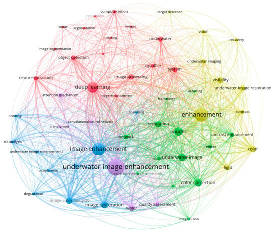
Figure 21.
Cluster analysis diagram of underwater image enhancement keywords.
Figure 21 shows the map of underwater image enhancement keywords and the relationship between them; from the figure, we can see that the keyword ‘underwater image enhancement’ has the most occurrences, with a count of 417, followed closely by ‘image enhancement’ and “enhancement”. These three keywords belong to the same field, and if we merge them, the count is 1036. The second ranked keyword is ‘deep learning’, with a count of 226, followed by model, with a count of 168.
Table 4 shows the rankings of the top 15 keywords in terms of the number of occurrences or centrality.
Table 4.
Keyword rankings based on number of count or centrality.
In the list of keywords ranked by quantity, the keywords ‘Color correction’, ‘Feature extraction’, etc., are listed as professional terms in the field of underwater images, which appeared earlier and belonged to the early traditional methods of enhancement. The deep learning keyword attracts the most attention, which appears in the latest year but has a high keyword frequency and indicates that this represents a new type of research trend. We further narrowed down the scope by limiting the keywords to 2020 and beyond, and the results are obtained in Table 4.
In Table 5, we find that in addition to the keywords of deep learning, attentional mechanism, convolutional neural network, generative adversarial network, unsupervised learning, and other keywords about deep learning are frequently occurring keywords; deep learning becomes the main force of underwater image enhancement after 2020, and the research direction gradually changes from traditional physical methods to deep learning methods.
Table 5.
Keyword rankings based on number of count or centrality after 2020.
Figure 22, produced via CiteSpace’s keyword mutation function, illustrates a visualization designed to examine the thematic evolution within a research domain. This analytical tool identifies shifts in core topics and emerging trends over time by evaluating changes in terminology across academic publications. Such evaluations enable scholars to detect critical transitions in a field’s focus, offering predictive insights into its developmental trajectory. By mapping temporal variations in keyword usage, this method not only highlights conceptual transformations but also aids in forecasting research priorities, thereby informing strategic directions for future scholarly inquiry.
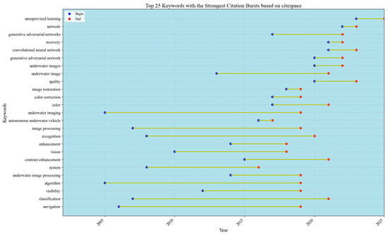
Figure 22.
Top 25 keywords with the strongest citation bursts based on CiteSpace.
Burst detection analysis offers a powerful approach for monitoring disciplinary trends, as it can effectively pinpoint sudden shifts in keyword activity. This method surpasses traditional bibliometric measures, such as citation counts or publication numbers, in its ability to capture the evolution of emerging research frontiers.
In the keyword mutation table in Figure 22, we find that the keywords algorithm, classification, navigation, etc., have a long time span and appear early, which suggests that researchers focused on some traditional physical algorithms for image restoration before 2020, and these algorithms have been a research hotspot. However, the keyword unsupervised learning has a high mutation intensity in recent years, and the intensity of other directions is weakening, which indicates that underwater image enhancement is shifting in the direction of unsupervised learning, which also confirms our previous conclusions that the field of underwater image enhancement is moving towards the development of the field in the deep learning direction.
4. Deep Learning Theory
In recent years, deep learning technology has brought breakthroughs in the field of underwater image enhancement through its unique paradigm innovation. Compared with traditional methods that rely on physical modeling, the core advantages of deep learning are reflected in three aspects: first, based on the end-to-end learning architecture [94], the deep network is able to automatically learn the complex mapping relationship from degraded images to clear images, getting rid of the strong dependence on physical models such as the Jaffe–McGlamery model, and effectively solving the problem of error accumulation in traditional methods due to simplifying the optical transmission equation, which leads to the problem of error accumulation [95]. Secondly, the multi-scale feature fusion mechanism enables the network to simultaneously handle multimodal tasks such as color offset correction [81,96], local contrast enhancement, and scattering noise suppression [97], breaking through the efficiency bottleneck of the traditional method that needs to deal with different types of degradation in tandem at different stages [98]. More importantly, the deep neural network can accurately portray the coupling relationship between non-uniform light distribution and spatially varying scattering effects in underwater environments through the stacking of nonlinear activation functions [99], which is significantly better than linear methods, such as histogram equalization, in complex scenarios, such as coral reef-shaded areas and turbid waters with sudden changes in visibility [100]. Together, these features drive the paradigm shift from ‘physics-driven’ to ‘data-driven’ underwater visual enhancement techniques [101], validated by benchmarks (UIEB [17], ImageNet [102]) and perceptual metrics (SSIM [103], LPIPS [104]).
4.1. Evolution: From CNNs to Transformers
Underwater image enhancement methodologies in the deep learning era have predominantly revolved around three core architectural frameworks. CNN-based approaches leverage hierarchical feature extraction capabilities [25], often enhanced by embedding physical priors into network layers [105,106,107]. GAN-driven solutions excel in modeling complex distribution mappings through adversarial training, particularly effective for unpaired data scenarios [108,109]. Transformer-based models, while relatively nascent in this domain, demonstrate superior performance in capturing long-range dependencies via self-attention mechanisms [110,111]. In Section 5, we present a comparative analysis of the operational characteristics of these models, highlighting their respective advantages in dealing with chromatic aberration, scattering noise, and non-uniform illumination.
4.1.1. CNN
In recent years, the rapid development of deep learning technology has driven a fundamental shift in underwater image enhancement from the traditional physical model-driven to data-driven paradigm. With its powerful feature extraction capability and end-to-end learning mechanism, convolutional neural networks (CNNs) gradually overcome the limitations of traditional methods relying on simplifying assumptions, and become a core tool for solving degradation problems such as color distortion, contrast degradation, and the blurring of details in underwater images. Figure 23 illustrates the structure of the CNN.
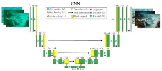
Figure 23.
Fundamental principles of CNN construction.
- a.
- Breakthrough in end-to-end multi-task learning frameworks
The UIE-Net proposed by Wang et al. [105] pioneered the construction of an end-to-end multi-task learning framework for the collaborative modeling of degraded features by jointly optimizing the color correction and defogging tasks. The network employs a pixel-shuffle strategy to enhance local feature extraction and synthesizes 200,000 training data based on a physical imaging model. Experiments show that its PSNR in the cross-scene test is improved by 23.5% compared with the traditional method, which verifies the effectiveness of multi-task learning.
- b.
- Normalization of benchmark datasets and baseline models
To overcome the limitation of data scarcity on algorithm evaluation, Li et al. further constructed the Underwater Image Enhancement Benchmark (UIEB) dataset, which contains 950 real underwater images (including 890 reference-degradation data pairs). The proposed water-net model based on this dataset adopts a progressive enhancement architecture and achieves a PSNR of 27.8 dB on UIEB, which is a 14.2% improvement over the earlier CNN model, through a three-stage feature fusion (degradation perception → adaptive enhancement → global optimization). This work provides a standardized benchmark for algorithm performance evaluation and model generalization capability [17].
- c.
- Multi-color spatial fusion and neural profile optimization
UIEC2-Net, proposed by Zhang et al., innovatively integrates the dual-color spaces of RGB and HSV to break through the representation limitations of a single-color space. Its architecture contains three core modules:
(1) RGB pixel-level module: denoising and color bias correction through residual linkage;
(2) HSV global adjustment module: introducing a neural curve layer to dynamically adjust brightness and saturation;
(3) Attention fusion module: weighted fusion of bispace outputs to suppress cross-modal conflicts.
Experiments show that the method achieves 3.85 on the UCIQE metric, which is a 12.7% improvement over the single-space model, verifying the superiority of multimodal feature fusion [106].
- d.
- Co-optimization of lightweight design and attention mechanism
Aiming at the balance between computational efficiency and detail retention, Zheng et al. proposed an improved CNN defogging network, the innovations of which include depth-separable convolution, with a 58% reduction in the amount of parameters (Equations (25)–(28)); basic attention module (BAM), focusing on key regions through channel-space dual paths; and cross-layer connection and pooling pyramid, enhancing multi-scale feature extraction.
The model reduces latency to 85 ms in 1080p image processing while maintaining UIQM 4.02, providing a viable solution for real-time underwater enhancement [107].
- e.
- Scene a priori-driven and video enhancement extensions
The UWCNN developed by Wang et al. for the first time embeds an underwater scene prior to the CNN training process to synthesize diverse degraded data (covering five types of water quality conditions) through a physical model. Their lightweight network (only 2.1 M parameters) employs a codec structure that incorporates jump connections to retain low-frequency information. Experiments show that the model achieves a PSNR of 26.5 dB in turbid waters with NTU > 30 and can be extended to video frame-by-frame enhancement with a stable frame rate of 25 fps [112].
4.1.2. GAN
Generative adversarial networks (GANs) have demonstrated significant advantages in the field of underwater image enhancement, gradually overcoming the limitations of traditional methods relying on simplifying assumptions through the deep integration of their adversarial learning mechanisms with physical models. GAN architectures (e.g., PUGAN, UW-CycleGAN) are able to simultaneously model complex light absorption-scattering effects through the dynamic game of the generator discriminator, and produce visually realistic enhancement results, which significantly improves the physical plausibility of color correction and the robustness of detail recovery. Figure 24 illustrates the structure of the GAN.
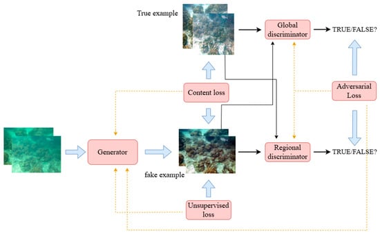
Figure 24.
Fundamental principles of GAN construction.
Cong et al. proposed an underwater image enhancement method based on generative adversarial networks (GANs) and physical models called the physical model-guided underwater image enhancement using GAN with dual discriminators. Underwater images usually suffer from low contrast, color distortion, and the blurring of details due to light absorption and scattering effects of the water medium, which increase the difficulty of underwater enhancement tasks. To solve these problems, PUGAN combines the visual aesthetics advantage of GANs and the scene adaptation advantage of physical models; consequently, an architecture (TSIE-subnet) and parameter estimation subnetwork (Par-subnet) are proposed. Par-subnet is used to learn the parameters of the inversion of the physical model and generate color-enhanced images as TSIE-subnet’s auxiliary information. The Degradation Quantization (DQ) module in the TSIE-subnet is used to quantify the scene degradation to enable the enhancement of critical regions. In addition, PUGAN is designed with dual discriminators for style–content adversarial constraints to improve the realism and visual aesthetics of the results [109].
Panetta et al. focused on the wide range of current target tracking methods on publicly available benchmark datasets and pointed out that these methods mainly focus on open space image data, while less attention has been paid to underwater visual data. The inherent distortion problems of color loss, poor contrast, and underexposure in underwater images due to light attenuation, refraction, and scattering in underwater environments greatly affect the visual quality of underwater data, making existing open-space trackers perform poorly on such data.
He presents the first comprehensive underwater target tracking benchmark dataset (UOT100), which aims to facilitate the development of tracking algorithms suitable for underwater environments. The dataset contains 104 underwater video sequences and over 74,000 annotated frames derived from natural and artificial underwater videos, covering a wide range of distortion types. The article also evaluates the performance of 20 state-of-the-art target tracking algorithms on this dataset and introduces a cascaded residual network for underwater image enhancement modeling to improve the accuracy and success of the tracker. The experimental results show that existing tracking algorithms have significant shortcomings on underwater data, while the generative adversarial network (GAN)-based augmentation model can significantly improve tracking performance [113].
Chen et al. explored the problem of low visual quality in underwater robots, an issue that limits their widespread application. Although several algorithms have been developed, real-time and adaptive approaches are still insufficient for practical tasks. To this end, the authors proposed a generative adversarial network (GAN)-based restoration scheme (GAN-RS), aiming to simultaneously preserve image content and remove underwater noise by means of a multi-branching discriminator (including adversarial and critic branches).
The authors not only employ adversarial learning, but also introduce a novel dark-channel a priori loss to facilitate the generator to produce more realistic visual effects. The authors also investigated the underwater index to characterize underwater features and designed an underwater index-based loss function to train the critical branch to suppress underwater noise [114].
Yan et al. proposed a model-driven cyclic coherent generative adversarial network (CycleGAN)-based model, called UW-CycleGAN, for underwater image restoration. The model is inspired by underwater image formation models and is capable of directly estimating the background light, transmission map, scene depth, and attenuation coefficient. Through comprehensive experiments, the authors demonstrate that the method outperforms other underwater image restoration methods both qualitatively and quantitatively, and is able to provide restored images with satisfactory color saturation and brightness [115].
Hambarde et al. proposed an end-to-end generative adversarial network called UW-GAN for depth estimation and image enhancement from a single underwater image. According to the literature, the coarse-grained depth map is firstly estimated by the underwater coarse-grained generative network (UWC-Net) and then the fine-grained depth map is computed by the underwater fine-grained network (UWF-Net), which splices the estimated coarse-grained depth map with the input image as an input. The UWF-Net consists of compression and excitation modules at both spatial and channel levesl for fine-grained depth estimation. In addition, the performance of the network proposed in the literature is analyzed on both real-world and synthetic underwater datasets and thoroughly evaluated on underwater images under different color dominance, contrast, and illumination conditions [116].
4.1.3. Transformer
The Transformer architecture is becoming an important technology paradigm in the field of underwater image enhancement due to its global modeling capability and self-attention mechanism. Compared with traditional convolutional neural networks (CNNs), Transformer can effectively capture the scattering effects of non-uniform illumination and spatial variations in underwater images through long-range dependent modeling (e.g., U-shape Transformer’s multi-scale windowed attention mechanism), which significantly improves the enhancement effect of complex scenes (e.g., shaded coral reefs and turbid waters). In addition, by combining physical a priori (e.g., Jaffe–McGlamery model) and frequency-domain guided optimization, Transformer shows stronger robustness in color correction and detail recovery. However, high computational complexity and high training data requirements are still the main challenges. Future research can explore a lightweight design (e.g., knowledge distillation) and multimodal fusion (e.g., sonar-optical cross-modal alignment) to further promote the practical application of Transformer in underwater enhancement. Figure 25 illustrates the structure of the Transformer.
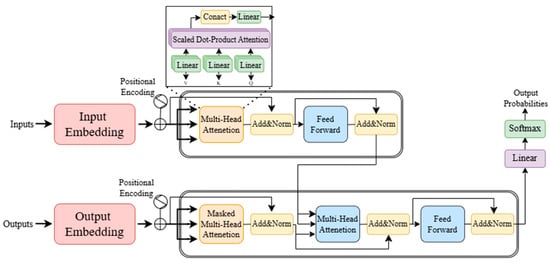
Figure 25.
Fundamental principles of Transformer construction.
Gao et al. proposed a path-enhanced Transformer framework called PE-Transformer, which aims to improve the performance of underwater object detection in complex backgrounds. The authors designed a scheme for embedding local path detection information that facilitates the interaction between high-level features and low-level features, thus enhancing the semantic representation of small-scale underwater targets. Within the CSWin-Transformer framework, rich dependencies are established between high-level and low-level features, further enhancing the semantic representation in the encoding stage. A flexible and adaptive point representation detection module is designed, which is capable of covering underwater targets from any direction. Through feature selection between salient point samples and points in classification and localization, the module achieves the optimization of feature selection while improving the detection accuracy of underwater objects [117].
Due to the absorption and scattering of underwater impurities, existing data-driven methods perform poorly in the absence of large-scale datasets and high-fidelity reference images. Peng et al. constructed a large-scale underwater image dataset (LSUI), which contains 4279 sets of real-world underwater images, each accompanied by clear reference images, semantic segmentation maps, and media transport maps.
On this basis, the authors introduced the Transformer model into the UIE task for the first time and proposed a U-shaped Transformer network. The network integrates two specially designed modules: the channel-level multi-scale feature fusion Transformer (CMSFFT) and the spatial-level global feature modeling Transformer (SGFMT). These modules enhance the network’s attention to heavily attenuated color channels and spatial regions.
In addition, to further enhance the contrast and saturation of the images, the authors designed a novel loss function combining RGB, LAB, and LCH color spaces, which follows the principles of human vision [110].
Shen et al. proposed an underwater image enhancement method based on a Dual Attention Transformer Block (DATB) called the UDAformer. Considering the inhomogeneity of underwater image degradation and the loss of color channels, UDAformer combines the Channel Self-Attention Transformer (CST) and the LCH loss function. The Self-Attention Transformer (CSAT) and Shifted Window Pixel Self-Attention Transformer (SW-PSAT) are also proposed in the literature; in these approaches, a new fusion method is proposed, combining channel and pixel self-attention for the efficient encoding and decoding of underwater image features. In addition, in order to improve computational efficiency, the literature also proposes a shift window method for pixel self-attention. Further, the self-attention weight matrix is computed by constructing a convolution, which enables the UDAformer to flexibly handle input images of various resolutions and reduce network parameters. Finally, underwater images are recovered by jump connections based on the design of an underwater imaging model [111].
Ummar et al. pointed out that the estimation of high-quality underwater images is an important step in the development of computer vision systems for marine environments, a step that encompasses many computer vision and robotics applications, such as ocean exploration, robotic manipulation, navigation, object detection, tracking, and marine life monitoring. To this end, Ummar et al. proposed a novel end-to-end underwater window transform generative adversarial network (UwTGAN). The algorithm consists of two main components: a transform generator for generating recovered underwater images and a transform discriminator for classifying the generated underwater images. Both components are equipped with window-based self-attention blocks (WSABs), which maximize efficiency and provide a relatively low computational cost by restricting the self-attention computation to non-overlapping local windows. The WSAB-based transform generator and discriminator are trained end-to-end, and the authors also formulate an efficient loss function to ensure that the variables are tightly integrated [118].
As a matter of fact, underwater image enhancement has evolved from relying on single-architecture deep learning models, such as CNNs for feature extraction, GANs for image generation, and Transformers for contextual understanding, to embracing fusion models that synergize these approaches. By integrating multiple architectures, these hybrid models mitigate the shortcomings of individual methods—such as CNNs’ limited global awareness, GANs’ training challenges, and Transformers’ computational costs—thereby achieving superior performance in enhancing underwater images.
Wang et al. proposed an underwater image enhancement method (UIE-Convformer) based on a convolutional neural network (CNN) with a feature fusion Transformer, which efficiently extracts the local texture features by the ConvBlock module and models the long range dependency by combining the cross-channel self-attention mechanism of the Feaformer module, which solves the problem of traditional CNNs concerning the difficulty in dealing with underwater wide-range blurring and scattering due to the restricted receptive field [119].
Zheng et al. proposed a dual generative adversarial network (LFT-DGAN) based on reversible convolutional decomposition with a full-frequency Transformer, which introduces reversible neural networks into underwater image processing for the first time, and separates the image into low, medium, and high-frequency components by the decomposition technique without information loss, to alleviate the problem of random information loss in the traditional mathematical transforms (such as wavelet transform). Experiments demonstrate that the method significantly outperforms existing methods in complex underwater scenarios such as UCCS, UIQS, etc., and shows strong generalization ability in extended tasks such as de-fogging and de-raining [120].
5. Comparison of Results
In this section, we perform a comparative analysis of traditional physical models, water-net, UWCNN, UWCycleGAN, U-shape, and so on. To further quantitatively assess the quality of the enhanced images, we calculated the peak signal-to-noise ratio (PSNR), underwater image quality measurement (UIQM), underwater contrast, and color enhancement quality evaluation (UCIQE, RGB statistics, and luminance metrics). The PSNR quantifies the signal-to-noise ratio of the image, with higher values indicating that the enhanced image has less distortion compared to the ideal image. the UCIQE mainly evaluates the color uniformity, contrast, and saturation of underwater images. UCIQE evaluates color uniformity, contrast, and saturation of underwater images, while UIQM is a comprehensive underwater image quality metric that combines contrast, hue, and sharpness.
Our experimental data come from the UIEB dataset, and in order to compare the performance of each deep learning model in different underwater scenarios, we selected three groups of experimental subjects from the dataset, namely, the rock group, the underwater portrait group, and the marine life group. Due to some hardware constraints, the training models we use are from pre-trained models without any processing. Since some models are only trained on 256 × 256 resolution, we choose the reference image as a medium grey image of the same size, and the PSNR values are for reference only.
The physical method (b) can more directly simulate the physical conditions underwater, and in some areas, especially those with moderate water turbidity or light, clearer images can be obtained. However, in cases of severe distortion, such as deep water with low visibility, enhancement may be less effective. Color correction may be too simple or impractical, as it may not capture the full effect of light in the water (Figure 26).

Figure 26.
Enhanced image of the rock group. (a) Original image; (b) physical; (c) UWCNN; (d) water-net; (e) UWCycleGAN; (f) U-shape; and (g) reference images (recognized as ground truth (GT).
The UWCNN (c) aims to address underwater image degradation more effectively. It generally improves visibility and restores more accurate colors, especially in shallow waters. However, in highly turbid waters or very deep seabed images, it may still have difficulty in restoring color and contrast. The color processing may be too biased towards certain shades and appear unnatural.
Water-net (d) ranks last in terms of brightness performance but improves contrast and reduces noise. It may work well in certain situations where contrast enhancement is needed without overdoing it.
UWCycleGAN (e) produces a natural, visually appealing image with more balanced colors and clearer details, and it ranks first among all methods in terms of brightness. However, it produces subtle artifacts with some color distortion (Table 6).
Table 6.
Average parameters for each type of rock group.
The U-shape method (f) is very effective in restoring structural details and reducing noise. This structure helps to maintain the sharpness of the image, making it an excellent choice for fine detail. It does introduce some unnatural artefacts, such as a slight halo effect around the edges of Picture 3 and the over-correction of colors, resulting in slightly ‘artificial’ or over-sharp results.
The physical model improves visibility and reproduces details extremely well for the first, third, and seventh images, close to the reference image (GT). However, the fourth images show severe overexposure, the colors look unnatural, the overcorrected appearance distorts the appearance of the scene, and its inability to deal with complex textures and fine details effectively produces an image that is inferior to the original image (Figure 27).

Figure 27.
Enhanced image of the human group. (a) Original image; (b) physical; (c) UWCNN; (d) water-net; (e) UWCycleGAN; (f) U-shape; and (g) GT.
UWCNN performs mediocrely in the human group; its ability to enhance brightness is still ranked at the bottom of the list, and UWCNN colors are prone to oversaturation or artifacts. The enhancement of Picture 3 is poor, its luminance, UCIQE, and UIQM are far below average, and there is almost no color representation. These problems are due to the limited ability of the model to handle complex underwater lighting conditions (Table 7).
Table 7.
Average parameters for each type of human group.
The water network has improved in areas such as color correction and object visibility. The model displayed a more natural fourth image with improved color accuracy. However, because of its average brightness performance, the model was sometimes unable to recover finer details, resulting in slight blurring in some areas.
UWCycleGAN, the luminance performance of which is at the top of the list, has visually enhanced images with realistic colors and details. This method performs well in maintaining a natural underwater environment. However, the first image is a bit overcorrected with the color of the third image, and some unnatural artifacts appear, especially at the boundaries of the objects.
The U-shape method performs best in improving the sharpness and contrast of the fourth image, which looks sharper and more detailed. However, the model sometimes has problems with tonality, resulting in unnatural gradients or overly bright areas, especially in the background, which can distract from the scene, as in images 3 and 7, which show an image that is too dark overall.
The physical models generally improve the visibility of fish and coral structures, with Figure 4 showing the best color reproduction of these models. The contrast between the fish and the background is better than in the original image. Colors are more vibrant, though not perfect, and there is a slight improvement in the clarity of the fish scales and water in particular (Figure 28).
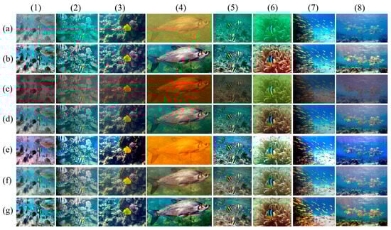
Figure 28.
Enhanced image of the underwater portrait group. (a) Original image; (b) physical; (c) UWCNN; (d) water-net; (e) UWCycleGAN; (f) U-shape; and (g) GT.
However, in Figure 1, the model gives the water a yellow–green tint that looks unnatural. Figure 3 shows some strange darkening in the background areas, especially around the coral structures, giving it an unrealistic look.
The texture of the UWCNN fish scales and corals is better preserved than the solid model, retaining detail, but the overall performance in the benthic organism group is also unsatisfactory, with the worst recovery of brightness, and a color treatment that may be too biased towards certain shades, which looks unnatural (Table 8).
Table 8.
Average parameters for each type of fish group.
The water-net method strikes a good balance between enhancing the image without oversaturating the colors. The fish and coral colors in columns two and seven look more natural. The coral areas and fish in images 4 and 7 look more like the ground truth, with more natural transitions between colors. Unlike the physical model, water-net seems to avoid the overexposure or darkening of certain areas, maintaining good overall brightness and visibility.
However, subtle artefacts can be seen around the fish in image 4, especially at the edges, which may be overcorrected by this method. The model sometimes struggles to maintain the finesse of the darker parts of the image (e.g., the background) and therefore can appear somewhat blurred.
UWCycleGAN shows significant improvement in color reproduction. Underwater visibility is much improved in images 3 and 7, and the background is much sharper compared to the original image. The water in the second column looks very close to the ground truth, with a natural blue color and no visible distortion.
Although the color balance has improved, the lighting in some areas (image 1) looks strange. There is an unnatural halo or strong contrast that reduces realism, and the overall photo has a strange pink color with some over-enhancement.
The U-shape method excels in just the right amount of color enhancement. Fish and corals, especially in pictures 2 and 3, appear more vibrant and detailed. The mode enhances contrast without creating noticeable artefacts. The fish are clearly defined, and the background appears brighter. There is a balance between natural and enhanced light: the lighting is more natural than other methods and helps to enhance realism. The fish in the first column is affected by the artificial lighting effect, where the light source does not match the distribution of natural light underwater, resulting in a slightly unrealistic feel.
6. Conclusions
Underwater image enhancement plays a pivotal role in marine resource exploration, ecological monitoring, and infrastructure inspection. This study systematically evaluates traditional physics-driven approaches and state-of-the-art deep learning models, revealing their distinct strengths, limitations, and applicability across diverse underwater environments. The key findings and implications are summarized as follows:
6.1. Comparative Performance of Physical and Deep Learning Models
- (a)
- Traditional Physical Models (e.g., simplified Jaffe–McGlamery)
Strengths: High interpretability, computational efficiency, and robustness in stable, shallow environments (depth < 10 m, NTU < 20). For instance, wavelength compensation and multi-scale histogram equalization effectively restore color balance and contrast (PSNR = 12.207 in rock group).
Limitations: performance degrades in complex scenarios (e.g., deep-sea or turbid waters) due to oversimplified assumptions (e.g., uniform background light) and an inability to model nonlinear degradation interactions (e.g., Figure 27b overexposure). Physical methods (e.g., wavelength compensation, Laplace sharpening) have difficulty in capturing the coupling effect between color deviation, scattered noise, and non-uniform illumination, resulting in overexposure (Figure 27b) or artifacts (Figure 28f) in complex scenes.
The fixed = 0.1, = 0.05, and = 0.03 used in our physical model are grounded in clear-water scenarios but lack justification for diverse depths and illumination conditions. This may contribute to overexposure or color distortion in complex scenes (e.g., Figure 27b).
- (b)
- Deep Learning Models
The water-net and UWCNN models excel in adaptive enhancement through supervised learning (UIEB dataset), balancing noise suppression and detail preservation. However, UWCNN struggles with luminance recovery (human group: luminance = 91.477), while water-net achieves moderate contrast improvement (UIQM = 0.205).
The UWCycleGAN and U-shape Transformer methods demonstrate superior capability in extreme conditions. UWCycleGAN’s adversarial training produces visually natural results (UCIQE = 30.565) but risks color oversaturation. The U-shape model, leveraging self-attention mechanisms, achieves state-of-the-art sharpness (rock group: luminance = 121.626), yet requires careful parameter tuning to avoid artifacts. Because of the hardware limitation, the training data are selected as pre-training data, while most deep learning models (e.g., UWCycleGAN, U-shape) are only trained at a 256 × 256 resolution, while real underwater devices (e.g., AUV, ROV) may acquire higher-resolution images (e.g., 1080p). Resolution normalization processing (e.g., downsampling) may lead to the loss of details, affecting the recovery of fine features such as coral texture, fish scales, etc. (Figure 26, Figure 27 and Figure 28).
6.2. Methodological Trade-Offs
- (a)
- Implementation Complexity
Physical models rely on explicit optical principles and minimal data, enabling real-time deployment on low-power devices (e.g., 15–20 MB memory for histogram equalization).
Deep learning methods demand substantial computational resources: water-net and UWCNN require mid-tier GPUs (25–30 fps), while Transformer-based models (U-shape) necessitate ≥8 GB VRAM, limiting edge-device applicability.
- (b)
- Interpretability
Physical models provide transparent enhancement steps (e.g., LAB color space analysis), aligning with optical principles.
They also lack transparency due to their black-box nature. While attention maps (e.g., U-shape’s multi-scale windows) partially reveal feature prioritization, the underlying decision-making process remains opaque. Hybrid approaches, such as embedding physical priors into network layers (e.g., UWCycleGAN’s dark-channel loss), improve interpretability but require extensive validation.
6.3. Practical Implications for Marine Applications
Shallow Waters: UWCycleGAN’s natural color rendering (Figure 26e) suits ecological monitoring in aquaculture ranches.
Deep-Sea Exploration: U-shape’s detail recovery (Figure 28f) aids structural inspection of subsea pipelines and cables.
Real-Time Systems: Lightweight CNNs (e.g., UWCNN) or physical models are preferable for continuous monitoring on underwater drones. While lightweight CNNs (e.g., UWCNN) and physical models are suggested as preferable for real-time monitoring on underwater drones, these recommendations are based on their computational efficiency in prior studies rather than direct measurements from our experiments, due to hardware limitations. As such, claims regarding real-time applicability are derived from theoretical analysis and the literature benchmarks.
6.4. Future Directions
Hybrid Frameworks: Integrating physical priors (e.g., transmission maps) into deep architectures (e.g., CNN preprocessing layers) could enhance robustness in turbid waters.
Lightweight Designs: Techniques like depth-wise separable convolutions or knowledge distillation (Section 4.1.1) should be prioritized to reduce latency (e.g., <50 ms for 1080p images). Although some real-time underwater image enhancement techniques are now available in academia [121,122,123,124], the trade-off between image quality and processing time remains a daunting task. Future research will focus on testing these models on more powerful hardware (e.g., mid-tier GPUs with ≥8 GB VRAM) to quantify real-time performance metrics such as FPS and latency. Collaborations with institutions possessing advanced computational resources are also planned to validate these capabilities.
Unsupervised Learning: Expanding synthetic datasets (e.g., LSUI) and leveraging contrastive learning frameworks can address data scarcity while improving cross-environment generalization.
Adaptive Enhancement: Dynamic strategy selection based on depth, turbidity, and hardware constraints will optimize resource utilization in marine ranching.
This study underscores that no single method universally outperforms others. The choice of enhancement technique must align with environmental conditions, task requirements, and hardware capabilities. Future innovations should focus on bridging the gap between physics-driven interpretability and data-driven adaptability, fostering sustainable advancements in underwater vision technologies. By addressing these challenges, we can unlock the full potential of underwater imaging for marine resource management, ecological conservation, and global blue economy development.
Author Contributions
Conceptualization, Y.M. and D.Z.; methodology, Y.M.; software, Y.M.; validation, Y.M. and Y.C.; formal analysis, Y.M.; investigation, Y.C.; resources, D.Z. and Y.M.; data curation, Y.M.; writing—review and editing, D.Z.; visualization, Y.M.; supervision, D.Z.; project administration, Y.M.; funding acquisition, Y.M. All authors have read and agreed to the published version of the manuscript.
Funding
This research received no external funding.
Data Availability Statement
All data generated and analyzed during this study are included in this published article. The datasets used and analyzed during the current study are available from the corresponding author on reasonable request.
Conflicts of Interest
The authors declare no conflicts of interest.
References
- Zhang, D.; Ma, Y.; Zhang, H.; Zhang, Y. Marine Equipment Siting Using Machine-Learning-Based Ocean Remote Sensing Data: Current Status and Future Prospects. Sustainability 2024, 16, 8889. [Google Scholar] [CrossRef]
- Bax, N.; Novaglio, C.; Maxwell, K.H.; Meyers, K.; McCann, J.; Jennings, S.; Frusher, S.; Fulton, E.A.; Nursey-Bray, M.; Fischer, M.; et al. Ocean resource use: Building the coastal blue economy. Rev. Fish Biol. Fish. 2021, 32, 189–207. [Google Scholar] [CrossRef]
- Zhang, D. Engineering Solutions to Mechanics, Marine Structures and Infrastructures. Eng. Solut. Mech. Mar. Struct. Infrastruct. 2024, 1. [Google Scholar] [CrossRef]
- Zhang, D.; Zhang, Y.; Zhao, B.; Ma, Y.; Si, K. Exploring subsea dynamics: A comprehensive review of underwater pipelines and cables. Phys. Fluids 2024, 36, 101304. [Google Scholar] [CrossRef]
- Levin, L.A.; Bett, B.J.; Gates, A.R.; Heimbach, P.; Howe, B.M.; Janssen, F.; McCurdy, A.; Ruhl, H.A.; Snelgrove, P.; Stocks, K.I.; et al. Global observing needs in the deep ocean. Front. Mar. Sci. 2019, 6, 241. [Google Scholar] [CrossRef]
- Yuan, B.; Cui, Y.; An, D.; Jia, Z.; Ding, W.; Yang, L. Marine environmental pollution and offshore aquaculture structure: Evidence from China. Front. Mar. Sci. 2023, 9, 979003. [Google Scholar] [CrossRef]
- Long, L.; Liu, H.; Cui, M.; Zhang, C.; Liu, C. Offshore aquaculture in China. Rev. Aquac. 2024, 16, 254–270. [Google Scholar] [CrossRef]
- Zhang, Y.; Li, T.; Lin, J.; Zhang, D. The Characteristics and Advantages of Deepwater Ultra-Large Marine Ranches. Eng. Solut. Mech. Mar. Struct. Infrastruct. 2024, 20, 20. [Google Scholar]
- Ma, Y.; Si, K.; Xie, Y.; Liang, Z.; Wu, J.; Zhang, D.; Zhang, Y.; Cai, R. Global Marine Ranching Research: Progress and Trends through Bibliometric Analysis. Eng. Solut. Mech. Mar. Struct. Infrastruct. 2024, 1, 1–23. [Google Scholar] [CrossRef]
- Holmer, M. Environmental issues of fish farming in offshore waters: Perspectives, concerns and research needs. Aquac. Environ. Interact. 2010, 1, 57–70. [Google Scholar] [CrossRef]
- Ubina, N.A.; Cheng, S.-C. A review of unmanned system technologies with its application to aquaculture farm monitoring and management. Drones 2022, 6, 12. [Google Scholar] [CrossRef]
- Tan, Y.; Lou, S. Research and development of a large-scale modern recreational fishery marine ranch System☆. Ocean Eng. 2021, 233, 108610. [Google Scholar] [CrossRef]
- Han, M.; Lyu, Z.; Qiu, T.; Xu, M. A review on intelligence dehazing and color restoration for underwater images. IEEE Trans. Syst. Man Cybern. Syst. 2018, 50, 1820–1832. [Google Scholar] [CrossRef]
- Zhou, J.-C.; Zhang, D.-H.; Zhang, W.-S. Classical and state-of-the-art approaches for underwater image defogging: A comprehensive survey. Front. Inf. Technol. Electron. Eng. 2020, 21, 1745–1769. [Google Scholar] [CrossRef]
- Porto Marques, T.; Branzan Albu, A.; Hoeberechts, M. A contrast-guided approach for the enhancement of low-lighting underwater images. J. Imaging 2019, 5, 79. [Google Scholar] [CrossRef]
- Zhou, J.; Zhang, D.; Zhang, W. A multifeature fusion method for the color distortion and low contrast of underwater images. Multimed. Tools Appl. 2021, 80, 17515–17541. [Google Scholar] [CrossRef]
- Li, C.; Guo, C.; Ren, W.; Cong, R.; Hou, J.; Kwong, S.; Tao, D. An underwater image enhancement benchmark dataset and beyond. IEEE Trans. Image Process. 2019, 29, 4376–4389. [Google Scholar] [CrossRef]
- Ancuti, C.O.; Ancuti, C.; De Vleeschouwer, C.; Bekaert, P. Color balance and fusion for underwater image enhancement. IEEE Trans. Image Process. 2017, 27, 379–393. [Google Scholar] [CrossRef]
- Garg, D.; Garg, N.K.; Kumar, M. Underwater image enhancement using blending of CLAHE and percentile methodologies. Multimed. Tools Appl. 2018, 77, 26545–26561. [Google Scholar] [CrossRef]
- Yang, M.; Hu, J.; Li, C.; Rohde, G.; Du, Y.; Hu, K. An in-depth survey of underwater image enhancement and restoration. IEEE Access 2019, 7, 123638–123657. [Google Scholar] [CrossRef]
- Hou, G.; Zhao, X.; Pan, Z.; Yang, H.; Tan, L.; Li, J. Benchmarking underwater image enhancement and restoration, and beyond. IEEE Access 2020, 8, 122078–122091. [Google Scholar] [CrossRef]
- Zhang, W.; Wang, Y.; Li, C. Underwater image enhancement by attenuated color channel correction and detail preserved contrast enhancement. IEEE J. Ocean. Eng. 2022, 47, 718–735. [Google Scholar] [CrossRef]
- Guo, Y.; Li, H.; Zhuang, P. Underwater image enhancement using a multiscale dense generative adversarial network. IEEE J. Ocean. Eng. 2019, 45, 862–870. [Google Scholar] [CrossRef]
- Schettini, R.; Corchs, S. Underwater image processing: State of the art of restoration and image enhancement methods. EURASIP J. Adv. Signal Process. 2010, 2010, 746052. [Google Scholar] [CrossRef]
- He, K.; Zhang, X.; Ren, S.; Sun, J. Deep residual learning for image recognition. In Proceedings of the IEEE Conference on Computer Vision and Pattern Recognition, Las Vegas, NV, USA, 27–30 June 2016. [Google Scholar]
- Li, J.; Skinner, K.A.; Eustice, R.M.; Johnson-Roberson, M. WaterGAN: Unsupervised generative network to enable real-time color correction of monocular underwater images. IEEE Robot. Autom. Lett. 2017, 3, 387–394. [Google Scholar] [CrossRef]
- Talaat, F.M.; El-Sappagh, S.; Alnowaiser, K.; Hassan, E. Improved prostate cancer diagnosis using a modified ResNet50-based deep learning architecture. BMC Med. Inform. Decis. Mak. 2024, 24, 23. [Google Scholar] [CrossRef]
- Yuan, X.; Guo, L.; Luo, C.; Zhou, X.; Yu, C. A survey of target detection and recognition methods in underwater turbid areas. Appl. Sci. 2022, 12, 4898. [Google Scholar] [CrossRef]
- Han, Y.; Huang, L.; Hong, Z.; Cao, S.; Zhang, Y.; Wang, J. Deep supervised residual dense network for underwater image enhancement. Sensors 2021, 21, 3289. [Google Scholar] [CrossRef]
- Zhang, Z.; Yan, H.; Tang, K.; Duan, Y. MetaUE: Model-based meta-learning for underwater image enhancement. arXiv 2023, arXiv:2303.06543. [Google Scholar]
- Zhang, S.; Zhao, S.; An, D.; Li, D.; Zhao, R. MDNet: A fusion generative adversarial network for underwater image enhancement. J. Mar. Sci. Eng. 2023, 11, 1183. [Google Scholar] [CrossRef]
- Zhu, D. Underwater image enhancement based on the improved algorithm of dark channel. Mathematics 2023, 11, 1382. [Google Scholar] [CrossRef]
- Han, J.; Shoeiby, M.; Malthus, T.; Botha, E.; Anstee, J.; Anwar, S.; Wei, R.; Armin, M.A.; Li, H.; Petersson, L. Underwater image restoration via contrastive learning and a real-world dataset. Remote Sens. 2022, 14, 4297. [Google Scholar] [CrossRef]
- Li, C.-Y.; Guo, J.-C.; Cong, R.-M.; Pang, Y.-W.; Wang, B. Underwater image enhancement by dehazing with minimum information loss and histogram distribution prior. IEEE Trans. Image Process. 2016, 25, 5664–5677. [Google Scholar] [CrossRef]
- Guo, C.; Li, C.; Guo, J.; Loy, C.C.; Hou, J.; Kwong, S.; Cong, R. Zero-reference deep curve estimation for low-light image enhancement. In Proceedings of the IEEE/CVF Conference on Computer Vision and Pattern Recognition, Seattle, WA, USA, 13–19 June 2020. [Google Scholar]
- Wei, K.; Fu, Y.; Zheng, Y.; Yang, J. Physics-based noise modeling for extreme low-light photography. IEEE Trans. Pattern Anal. Mach. Intell. 2021, 44, 8520–8537. [Google Scholar] [CrossRef]
- Lee, S.-W.; Maik, V.; Jang, J.; Shin, J.; Paik, J. Noise-adaptive spatio-temporal filter for real-time noise removal in low light level images. IEEE Trans. Consum. Electron. 2005, 51, 648–653. [Google Scholar] [CrossRef]
- Li, C.; Tang, S.; Kwan, H.K.; Yan, J.; Zhou, T. Color correction based on cfa and enhancement based on retinex with dense pixels for underwater images. IEEE Access 2020, 8, 155732–155741. [Google Scholar] [CrossRef]
- Cheng, F.-H.; Hsu, W.-H.; Chen, T.-W. Recovering colors in an image with chromatic illuminant. IEEE Trans. Image Process. 1998, 7, 1524–1533. [Google Scholar] [CrossRef]
- Wang, B.; Wei, B.; Kang, Z.; Hu, L.; Li, C. Fast color balance and multi-path fusion for sandstorm image enhancement. Signal Image Video Process. 2021, 15, 637–644. [Google Scholar] [CrossRef]
- Guo, Z.; Wang, B.; Li, C. CAT: A lightweight Color-aware transformer for sandstorm image enhancement. Displays 2024, 83, 102714. [Google Scholar] [CrossRef]
- Yang, M.; Hu, K.; Du, Y.; Wei, Z.; Sheng, Z.; Hu, J. Underwater image enhancement based on conditional generative adversarial network. Signal Process. Image Commun. 2020, 81, 115723. [Google Scholar] [CrossRef]
- Susstrunk, S.E.; Winkler, S. Color image quality on the internet. Internet Imaging V 2003, 5304, 118–131. [Google Scholar]
- Yuan, W.; Poosa, S.R.P.; Dirks, R.F. Comparative analysis of color space and channel, detector, and descriptor for feature-based image registration. J. Imaging 2024, 10, 105. [Google Scholar] [CrossRef]
- Kanan, C.; Cottrell, G.W. Color-to-grayscale: Does the method matter in image recognition? PLoS ONE 2012, 7, e29740. [Google Scholar] [CrossRef]
- Güneş, A.; Kalkan, H.; Durmuş, E. Optimizing the color-to-grayscale conversion for image classification. Signal Image Video Process. 2016, 10, 853–860. [Google Scholar] [CrossRef]
- Sowmya, V.; Govind, D.; Soman, K.P. Significance of incorporating chrominance information for effective color-to-grayscale image conversion. Signal Image Video Process. 2017, 11, 129–136. [Google Scholar] [CrossRef]
- Gonzalez, R.C.; Woods, R.E. Digital Image Processing, 4th ed.; Pearson Education: Rotherham, UK, 2002; ISBN 978-0-13-335672-4. [Google Scholar]
- Wang, G.; Li, W.; Gao, X.; Xiao, B.; Du, J. Functional and anatomical image fusion based on gradient enhanced decomposition model. IEEE Trans. Instrum. Meas. 2022, 71, 2508714. [Google Scholar] [CrossRef]
- Yang, Y.; Park, D.S.; Huang, S.; Rao, N. Medical image fusion via an effective wavelet-based approach. EURASIP J. Adv. Signal Process. 2010, 2010, 579341. [Google Scholar] [CrossRef]
- Suresha, R.; Jayanth, R.; Shriharikoushik, M.A. Computer vision approach for motion blur image restoration system. In Proceedings of the 2023 14th International Conference on Computing Communication and Networking Technologies (ICCCNT), Delhi, India, 6–8 July 2023. [Google Scholar]
- Wang, W.; Li, Z.; Wu, S.; Zeng, L. Hazy image decolorization with color contrast restoration. IEEE Trans. Image Process. 2019, 29, 1776–1787. [Google Scholar] [CrossRef]
- Dong, L.; Zhang, W.; Xu, W. Underwater image enhancement via integrated RGB and LAB color models. Signal Process. Image Commun. 2022, 104, 116684. [Google Scholar] [CrossRef]
- Cernadas, E.; Fernández-Delgado, M.; González-Rufino, E.; Carrión, P. Influence of normalization and color space to color texture classification. Pattern Recognit. 2017, 61, 120–138. [Google Scholar] [CrossRef]
- Burambekova, A.; Pakizar, S. Comparative analysis of color models for human perception and visual color difference. arXiv 2024, arXiv:2406.19520. [Google Scholar]
- Reinhard, E.; Adhikhmin, M.; Gooch, B.; Shirley, P. Color transfer between images. IEEE Comput. Graph. Appl. 2001, 21, 34–41. [Google Scholar] [CrossRef]
- Song, Y.; Nakath, D.; She, M.; Köser, K. Optical imaging and image restoration techniques for deep ocean mapping: A comprehensive survey. PFG–J. Photogramm. Remote Sens. Geoinf. Sci. 2022, 90, 243–267. [Google Scholar] [CrossRef]
- Lin, S.; Ning, Z.; Zhang, R. Modified optical model and optimized contrast for underwater image restoration. Opt. Commun. 2025, 574, 130942. [Google Scholar] [CrossRef]
- He, K.; Jian, S.; Xiaoou, T. Single image haze removal using dark channel prior. IEEE Trans. Pattern Anal. Mach. Intell. 2010, 33, 2341–2353. [Google Scholar]
- Jansen, H.; Bogaart, L.v.D.; Hommersom, A.; Capelle, J. Spatio-temporal analysis of sediment plumes formed by mussel fisheries and aquaculture in the western Wadden Sea. Aquac. Environ. Interact. 2023, 15, 145–159. [Google Scholar] [CrossRef]
- Jaffe, J. Computer modeling and the design of optimal underwater imaging systems. IEEE J. Ocean. Eng. 1990, 15, 101–111. [Google Scholar] [CrossRef]
- Mobley, C.D. Light and Water: Radiative Transfer in Natural Waters; Academic Press: San Diego, CA, USA, 1994; ISBN 978-0125027502. [Google Scholar]
- Twardowski, M.S.; Boss, E.; Macdonald, J.B.; Pegau, W.S.; Barnard, A.H.; Zaneveld, J.R.V. A model for estimating bulk refractive index from the optical backscattering ratio and the implications for understanding particle composition in case I and case II waters. J. Geophys. Res. Oceans 2001, 106, 14129–14142. [Google Scholar] [CrossRef]
- Kirk, J.T. Light and Photosynthesis in Aquatic Ecosystems; Cambridge University press: Cambridge, UK, 1994. [Google Scholar]
- Shafuda, F.; Kondo, H. A simple method for backscattered light estimation and image restoration in turbid water. In Proceedings of the OCEANS 2021: San Diego–Porto, San Diego, CA, USA, 20–23 September 2021; IEEE: Piscataway, NJ, USA, 2021; pp. 1–6. [Google Scholar]
- Piskozub, J.; Stramski, D.; Terrill, E.; Melville, W.K. Influence of forward and multiple light scatter on the measurement of beam attenuation in highly scattering marine environments. Appl. Opt. 2004, 43, 4723–4731. [Google Scholar] [CrossRef]
- Garaba, S.P.; Voß, D.; Zielinski, O. Physical, bio-optical state and correlations in North–Western European Shelf Seas. Remote Sens. 2014, 6, 5042–5066. [Google Scholar] [CrossRef]
- Trucco, E.; Olmos-Antillon, A. Self-tuning underwater image restoration. IEEE J. Ocean. Eng. 2006, 31, 511–519. [Google Scholar] [CrossRef]
- Ji, K.; Lei, W.; Zhang, W. A deep Retinex network for underwater low-light image enhancement. Mach. Vis. Appl. 2023, 34, 122. [Google Scholar] [CrossRef]
- Jin, Y.; Fayad, L.M.; Laine, A.F. Contrast enhancement by multiscale adaptive histogram equalization. Wavelets Appl. Signal Image Process. IX 2001, 4478, 206–214. [Google Scholar]
- Huang, S.; Li, D.; Zhao, W.; Liu, Y. Haze removal algorithm for optical remote sensing image based on multi-scale model and histogram characteristic. IEEE Access 2019, 7, 104179–104196. [Google Scholar] [CrossRef]
- Zhang, W.; Li, X.; Xu, S.; Li, X.; Yang, Y.; Xu, D.; Liu, T.; Hu, H. Underwater image restoration via adaptive color correction and contrast enhancement fusion. Remote Sens. 2023, 15, 4699. [Google Scholar] [CrossRef]
- Wang, H.; Sun, S.; Ren, P. Underwater color disparities: Cues for enhancing underwater images toward natural color consistencies. IEEE Trans. Circuits Syst. Video Technol. 2023, 34, 738–753. [Google Scholar] [CrossRef]
- Chiang, J.Y.; Chen, Y.-C. Underwater image enhancement by wavelength compensation and dehazing. IEEE Trans. Image Process. 2011, 21, 1756–1769. [Google Scholar] [CrossRef]
- Zhou, J.; Zhang, D.; Ren, W.; Zhang, W. Auto color correction of underwater images utilizing depth information. IEEE Geosci. Remote Sens. Lett. 2022, 19, 1504805. [Google Scholar] [CrossRef]
- Zhou, J.; Zhang, D.; Zhang, W. Underwater image enhancement method via multi-feature prior fusion. Appl. Intell. 2022, 52, 16435–16457. [Google Scholar] [CrossRef]
- Ke, K.; Zhang, B.; Zhang, C.; Yao, B.; Guo, S.; Tang, F. Underwater image enhancement via color correction and multi-feature image fusion. Meas. Sci. Technol. 2024, 35, 096123. [Google Scholar] [CrossRef]
- Shang, J.; Li, Y.; Xing, H.; Yuan, J. LGT: Luminance-guided transformer-based multi-feature fusion network for underwater image enhancement. Inf. Fusion 2025, 118, 102977. [Google Scholar] [CrossRef]
- Zhou, J.; Sun, J.; Zhang, W.; Lin, Z. Multi-view underwater image enhancement method via embedded fusion mechanism. Eng. Appl. Artif. Intell. 2023, 121, 105946. [Google Scholar] [CrossRef]
- Yin, M.; Du, X.; Liu, W.; Yu, L.; Xing, Y. Multiscale fusion algorithm for underwater image enhancement based on color preservation. IEEE Sens. J. 2023, 23, 7728–7740. [Google Scholar] [CrossRef]
- Chen, R.; Cai, Z.; Cao, W. MFFN: An underwater sensing scene image enhancement method based on multiscale feature fusion network. IEEE Trans. Geosci. Remote Sens. 2021, 60, 4205612. [Google Scholar] [CrossRef]
- Oren, M.; Nayar, S.K. Generalization of the Lambertian model and implications for machine vision. Int. J. Comput. Vis. 1995, 14, 227–251. [Google Scholar] [CrossRef]
- Tomasi, C.; Manduchi, R. Bilateral filtering for gray and color images. In Proceedings of the Sixth International Conference on Computer Vision, Bombay, India, 7 January 1998. [Google Scholar]
- Gavaskar, R.G.; Chaudhury, K.N. Fast adaptive bilateral filtering. IEEE Trans. Image Process. 2018, 28, 779–790. [Google Scholar] [CrossRef]
- Chen, B.H.; Tseng, Y.S.; Yin, J.L. Gaussian-adaptive bilateral filter. IEEE Signal Process. Lett. 2020, 27, 1670–1674. [Google Scholar] [CrossRef]
- Bianco, G.; Muzzupappa, M.; Bruno, F.; Garcia, R.; Neumann, L. A new color correction method for underwater imaging. Int. Arch. Photogramm. Remote Sens. Spat. Inf. Sci. 2015, 40, 25–32. [Google Scholar] [CrossRef]
- Song, W.; Wang, Y.; Huang, D.; Liotta, A.; Perra, C. Enhancement of underwater images with statistical model of background light and optimization of transmission map. IEEE Trans. Broadcast. 2020, 66, 153–169. [Google Scholar] [CrossRef]
- Gan, W.; Wu, X.; Wu, W.; Yang, X.; Ren, C.; He, X.; Liu, K. Infrared and visible image fusion with the use of multi-scale edge-preserving decomposition and guided image filter. Infrared Phys. Technol. 2015, 72, 37–51. [Google Scholar] [CrossRef]
- Burt, P.J.; Adelson, E.H. The Laplacian pyramid as a compact image code. In Readings in Computer Vision; Morgan Kaufmann: Burlington, MA, USA, 1987; pp. 671–679. [Google Scholar]
- Pajares, G.; De La Cruz, J.M. A wavelet-based image fusion tutorial. Pattern Recognit. 2004, 37, 1855–1872. [Google Scholar] [CrossRef]
- Li, S.; Kang, X.; Hu, J. Image fusion with guided filtering. IEEE Trans. Image Process. 2013, 22, 2864–2875. [Google Scholar] [PubMed]
- Mertens, T.; Kautz, J.; Van Reeth, F. Exposure fusion: A simple and practical alternative to high dynamic range photography. In Computer Graphics Forum; Blackwell Publishing Ltd.: Oxford, UK, 2009; Volume 28, pp. 161–171. [Google Scholar]
- Agarwala, A.; Dontcheva, M.; Agrawala, M.; Drucker, S.; Colburn, A.; Curless, B.; Salesin, D.; Cohen, M. Interactive digital photomontage. In ACM SIGGRAPH 2004 Papers; University of Washington: Seattle, WA, USA, 2004; pp. 294–302. [Google Scholar]
- Ronneberger, O.; Fischer, P.; Brox, T. U-net: Convolutional networks for biomedical image segmentation. In Medical Image Computing and Computer-Assisted Intervention–MICCAI 2015: 18th International Conference, Munich, Germany, 5–9 October 2015, Proceedings, Part III 18; Springer International Publishing: Cham, Switzerland, 2015. [Google Scholar]
- Anwar, S.; Li, C.; Porikli, F. Deep underwater image enhancement. arXiv 2018, arXiv:1807.03528. [Google Scholar]
- Qi, Q.; Li, K.; Zheng, H.; Gao, X.; Hou, G.; Sun, K. SGUIE-Net: Semantic attention guided underwater image enhancement with multi-scale perception. IEEE Trans. Image Process. 2022, 31, 6816–6830. [Google Scholar] [CrossRef]
- Li, C.; Anwar, S.; Hou, J.; Cong, R.; Guo, C.; Ren, W. Underwater image enhancement via medium transmission-guided multi-color space embedding. IEEE Trans. Image Process. 2021, 30, 4985–5000. [Google Scholar] [CrossRef]
- Qiao, N.; Dong, L.; Sun, C. Adaptive deep learning network with multi-scale and multi-dimensional features for underwater image enhancement. IEEE Trans. Broadcast. 2022, 69, 482–494. [Google Scholar] [CrossRef]
- Fabbri, C.; Islam, M.J.; Sattar, J. Enhancing underwater imagery using generative adversarial networks. In Proceedings of the 2018 IEEE International Conference on Robotics and Automation (ICRA), Brisbane, QLD, Australia, 21–25 May 2018. [Google Scholar]
- Candela, A.; Edelson, K.; Gierach, M.M.; Thompson, D.R.; Woodward, G.; Wettergreen, D. Using remote sensing and in situ measurements for efficient mapping and optimal sampling of coral reefs. Front. Mar. Sci. 2021, 8, 689489. [Google Scholar] [CrossRef]
- Zhu, J.-Y.; Park, T.; Isola, P.; Efros, A.A. Unpaired image-to-image translation using cycle-consistent adversarial networks. In Proceedings of the IEEE International Conference on Computer Vision, Venice, Italy, 22–29 October 2017; pp. 2223–2232. [Google Scholar]
- Deng, J.; Dong, W.; Socher, R.; Li, L.J.; Li, K.; Li, F. Imagenet: A large-scale hierarchical image database. In Proceedings of the 2009 IEEE Conference on Computer Vision and Pattern Recognition, Miami, FL, USA, 20–25 June 2009. [Google Scholar]
- Wang, Z.; Bovik, A.C.; Sheikh, H.R.; Simoncelli, E.P. Image quality assessment: From error visibility to structural similarity. IEEE Trans. Image Process. 2004, 13, 600–612. [Google Scholar] [CrossRef]
- Zhang, R.; Isola, P.; Efros, A.A.; Shechtman, E.; Wang, O. The unreasonable effectiveness of deep features as a perceptual metric. In Proceedings of the IEEE Conference on Computer Vision and Pattern Recognition, Salt Lake City, UT, USA, 18–23 June 2018. [Google Scholar]
- Wang, Y.; Zhang, J.; Cao, Y.; Wang, Z. A deep CNN method for underwater image enhancement. In Proceedings of the 2017 IEEE International Conference on Image Processing (ICIP), Beijing, China, 17–20 September 2017. [Google Scholar]
- Wang, Y.; Guo, J.; Gao, H.; Yue, H. UIEC^2-Net: CNN-based underwater image enhancement using two color space. Signal Process. Image Commun. 2021, 96, 116250. [Google Scholar] [CrossRef]
- Zheng, M.; Luo, W. Underwater image enhancement using improved CNN based defogging. Electronics 2022, 11, 150. [Google Scholar] [CrossRef]
- Wang, J.; Li, P.; Deng, J.; Du, Y.; Zhuang, J.; Liang, P.; Liu, P. CA-GAN: Class-condition attention GAN for underwater image enhancement. IEEE Access 2020, 8, 130719–130728. [Google Scholar] [CrossRef]
- Cong, R.; Yang, W.; Zhang, W.; Li, C.; Guo, C.-L.; Huang, Q.; Kwong, S. PUGAN: Physical model-guided underwater image enhancement using GAN with dual-discriminators. IEEE Trans. Image Process. 2023, 32, 4472–4485. [Google Scholar] [CrossRef] [PubMed]
- Peng, L.; Zhu, C.; Bian, L. U-shape transformer for underwater image enhancement. IEEE Trans. Image Process. 2023, 32, 3066–3079. [Google Scholar] [CrossRef] [PubMed]
- Shen, Z.; Xu, H.; Luo, T.; Song, Y.; He, Z. UDAformer: Underwater image enhancement based on dual attention transformer. Comput. Graph. 2023, 111, 77–88. [Google Scholar] [CrossRef]
- Li, C.; Anwar, S.; Porikli, F. Underwater scene prior inspired deep underwater image and video enhancement. Pattern Recognit. 2020, 98, 107038. [Google Scholar] [CrossRef]
- Panetta, K.; Kezebou, L.; Oludare, V.; Agaian, S. Comprehensive underwater object tracking benchmark dataset and underwater image enhancement with GAN. IEEE J. Ocean. Eng. 2021, 47, 59–75. [Google Scholar] [CrossRef]
- Chen, X.; Yu, J.; Kong, S.; Wu, Z.; Fang, X.; Wen, L. Towards real-time advancement of underwater visual quality with GAN. IEEE Trans. Ind. Electron. 2019, 66, 9350–9359. [Google Scholar] [CrossRef]
- Yan, H.; Zhang, Z.; Xu, J.; Wang, T.; An, P.; Wang, A.; Duan, Y. UW-CycleGAN: Model-driven CycleGAN for underwater image restoration. IEEE Trans. Geosci. Remote Sens. 2023, 61, 4207517. [Google Scholar] [CrossRef]
- Hambarde, P.; Murala, S.; Dhall, A. UW-GAN: Single-image depth estimation and image enhancement for underwater images. IEEE Trans. Instrum. Meas. 2021, 70, 5018412. [Google Scholar] [CrossRef]
- Gao, J.; Zhang, Y.; Geng, X.; Tang, H.; Bhatti, U.A. PE-Transformer: Path enhanced transformer for improving underwater object detection. Expert Syst. Appl. 2024, 246, 123253. [Google Scholar] [CrossRef]
- Ummar, M.; Dharejo, F.A.; Alawode, B.; Mahbub, T.; Piran, J.; Javed, S. Window-based transformer generative adversarial network for autonomous underwater image enhancement. Eng. Appl. Artif. Intell. 2023, 126, 107069. [Google Scholar] [CrossRef]
- Wang, B.; Xu, H.; Jiang, G.; Yu, M.; Ren, T.; Luo, T.; Zhu, Z. UIE-convformer: Underwater image enhancement based on convolution and feature fusion transformer. IEEE Trans. Emerg. Top. Comput. Intell. 2024, 8, 1952–1968. [Google Scholar] [CrossRef]
- Zheng, S.; Wang, R.; Zheng, S.; Wang, L.; Liu, Z. A learnable full-frequency transformer dual generative adversarial network for underwater image enhancement. Front. Mar. Sci. 2024, 11, 1321549. [Google Scholar] [CrossRef]
- Moghimi, M.K.; Mohanna, F. Real-time underwater image enhancement: A systematic review. J. Real-Time Image Process. 2021, 18, 1509–1525. [Google Scholar] [CrossRef]
- Banerjee, J.; Ray, R.; Vadali, S.R.K.; Shome, S.N.; Nandy, S. Real-time underwater image enhancement: An improved approach for imaging with AUV-150. Sadhana 2016, 41, 225–238. [Google Scholar] [CrossRef]
- Yang, H.; Xu, J.; Lin, Z.; He, J. LU2Net: A lightweight network for real-time underwater image enhancement. arXiv 2024, arXiv:2406.14973. [Google Scholar]
- Zhang, S.; Zhao, S.; An, D.; Li, D.; Zhao, R. LiteEnhanceNet: A lightweight network for real-time single underwater image enhancement. Expert Syst. Appl. 2024, 240, 122546. [Google Scholar] [CrossRef]
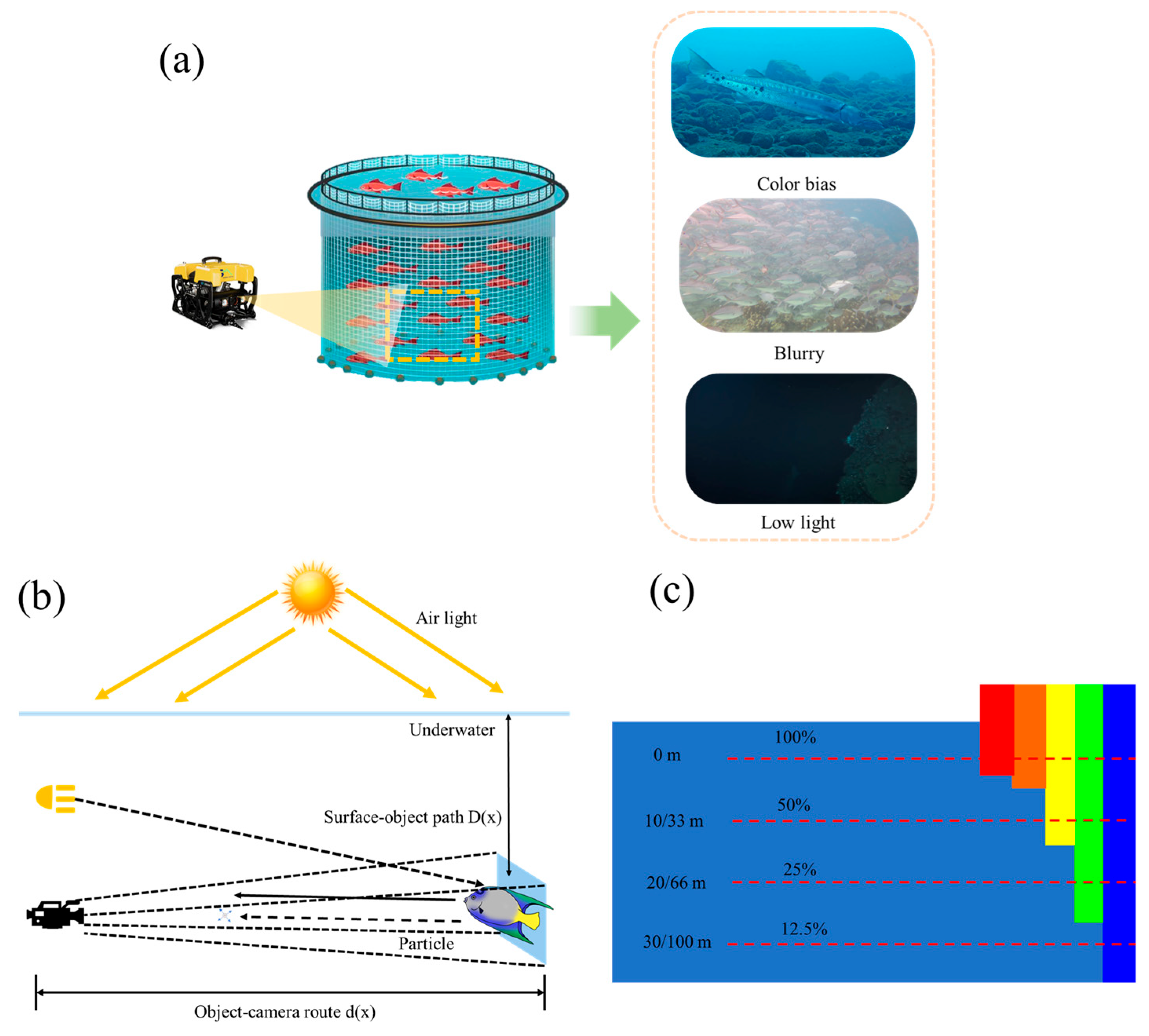
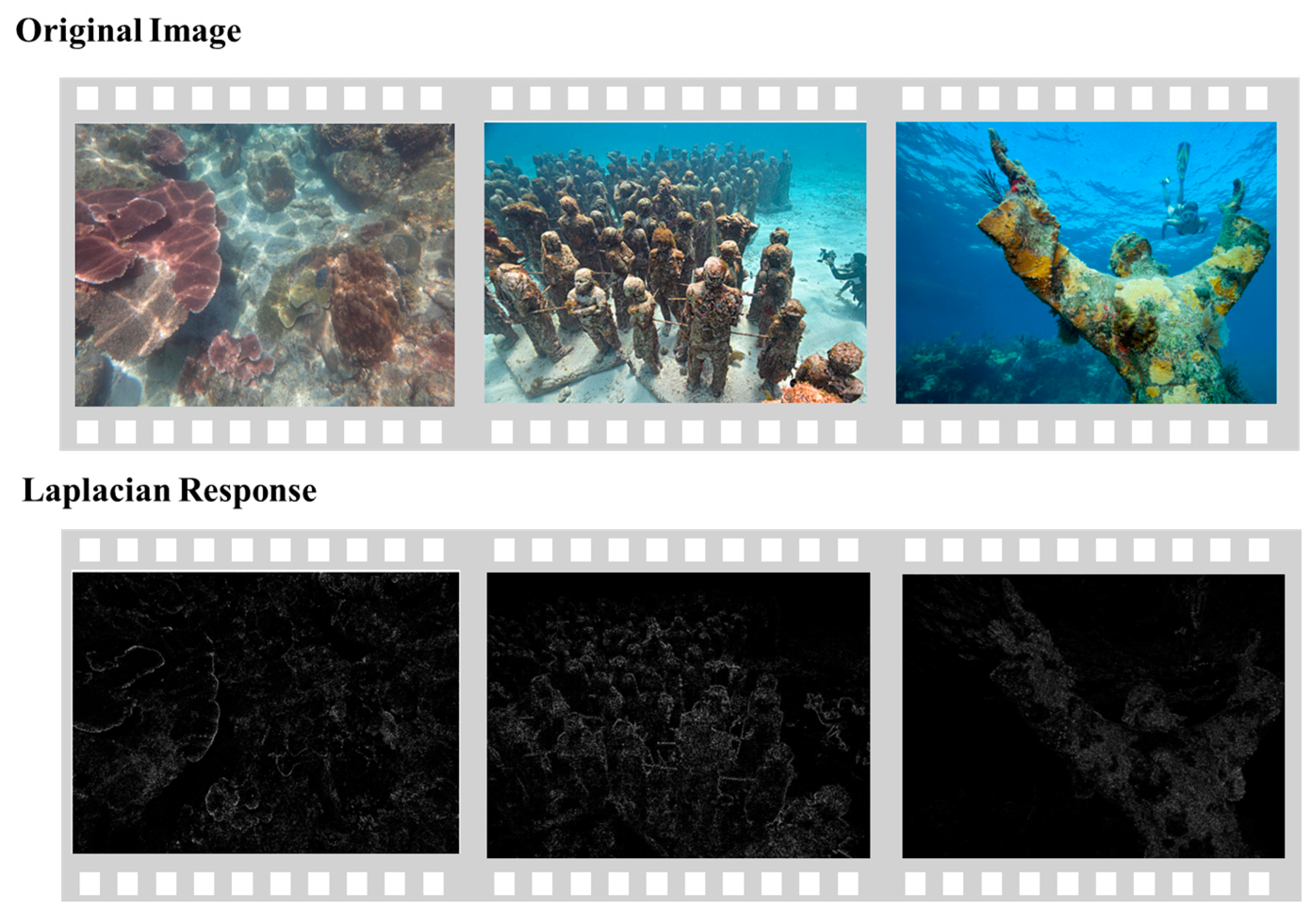
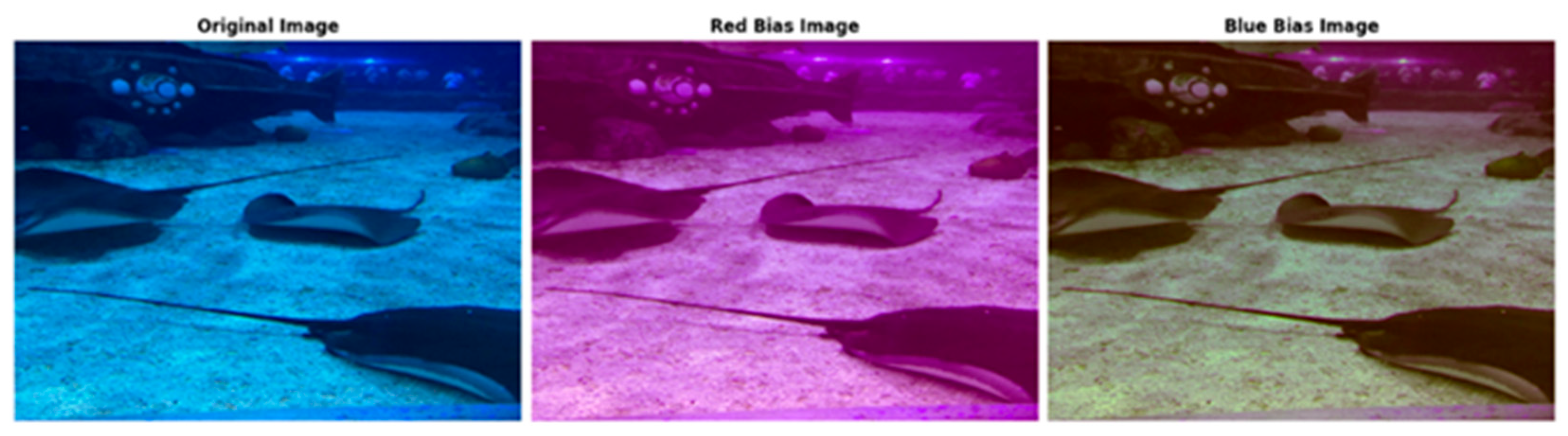
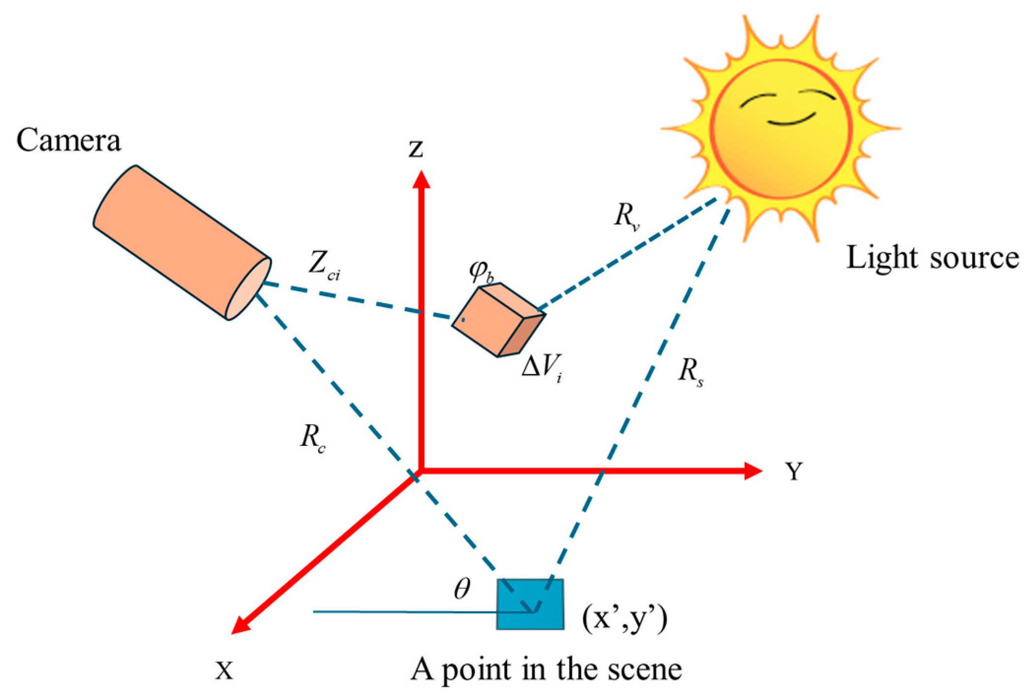
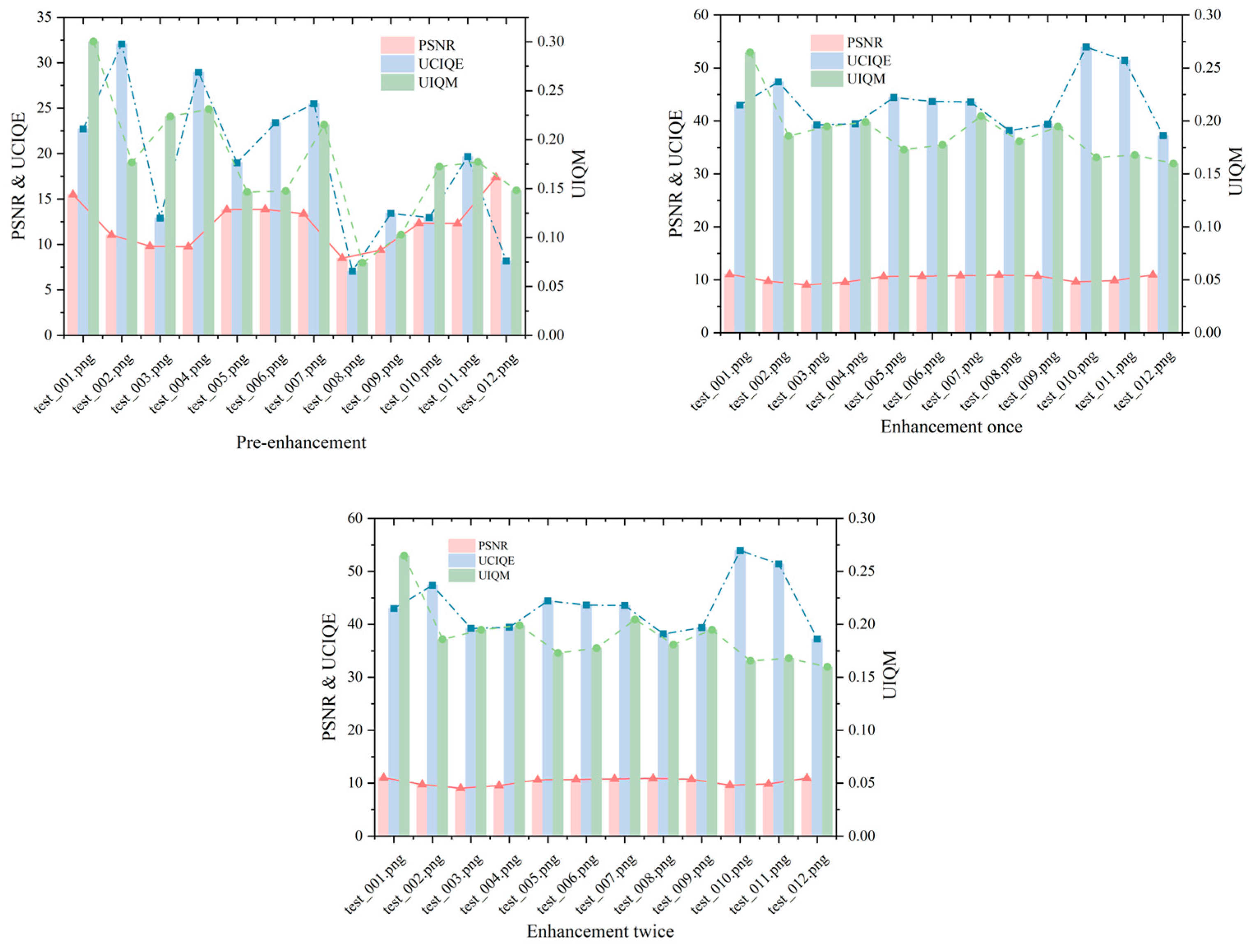
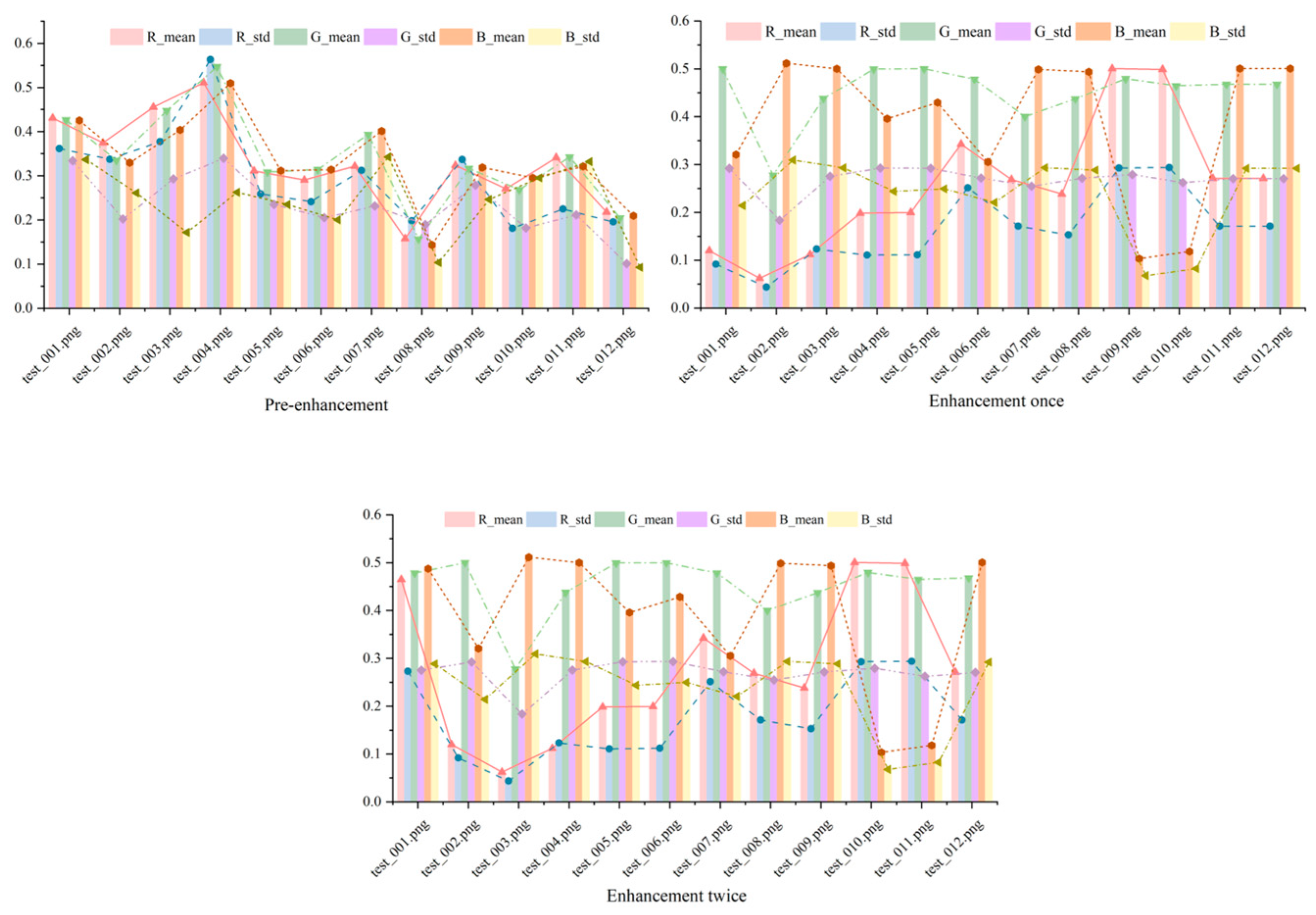
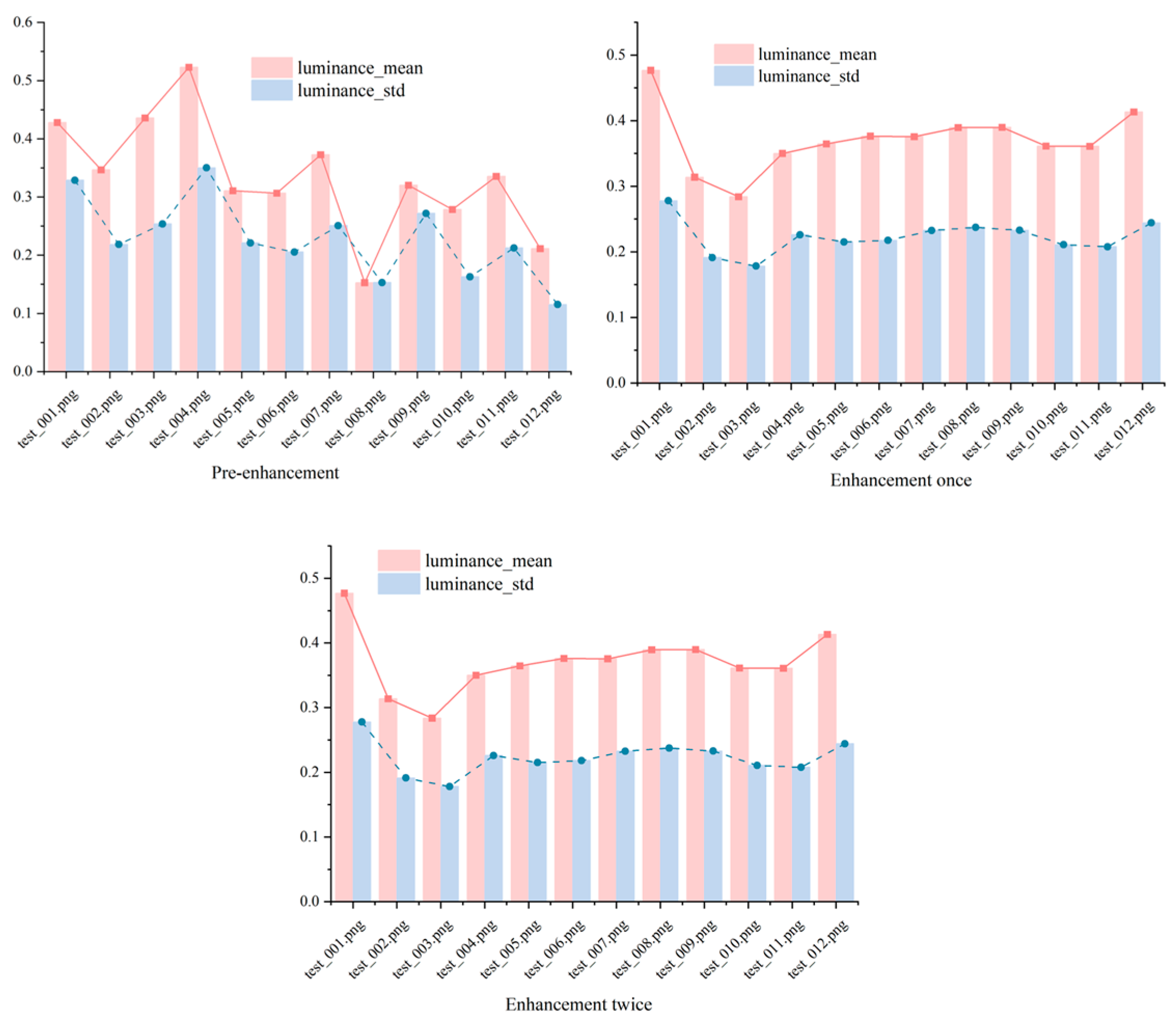
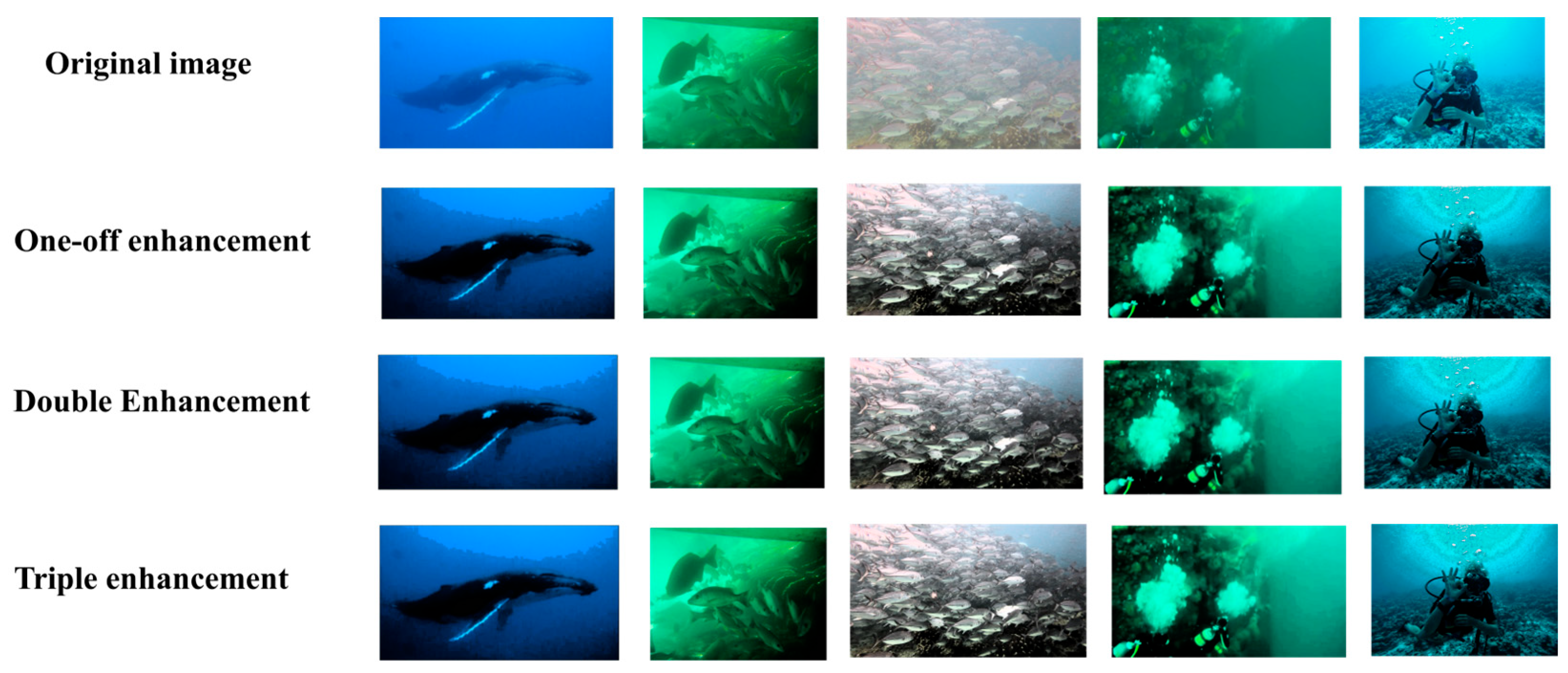
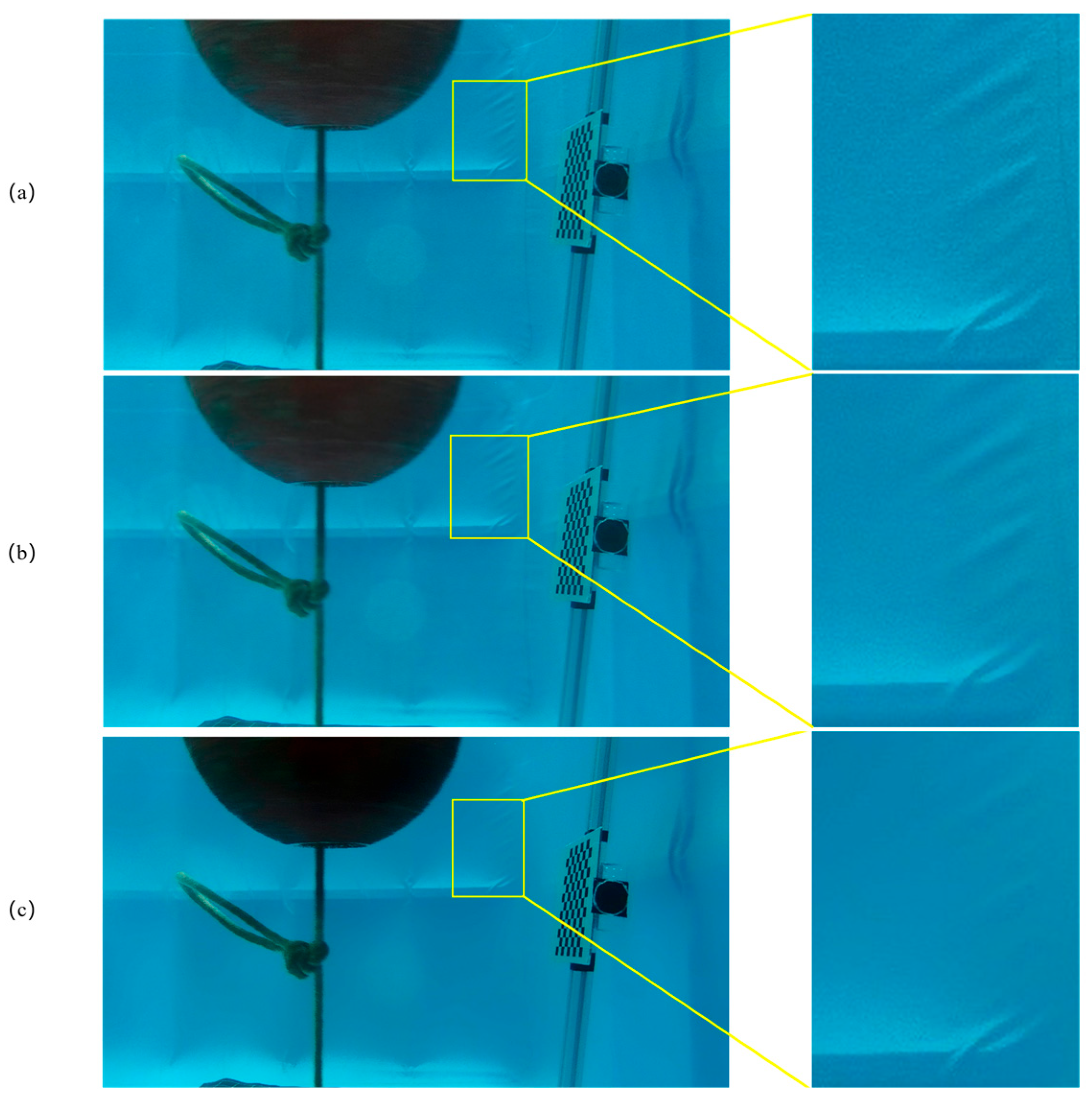
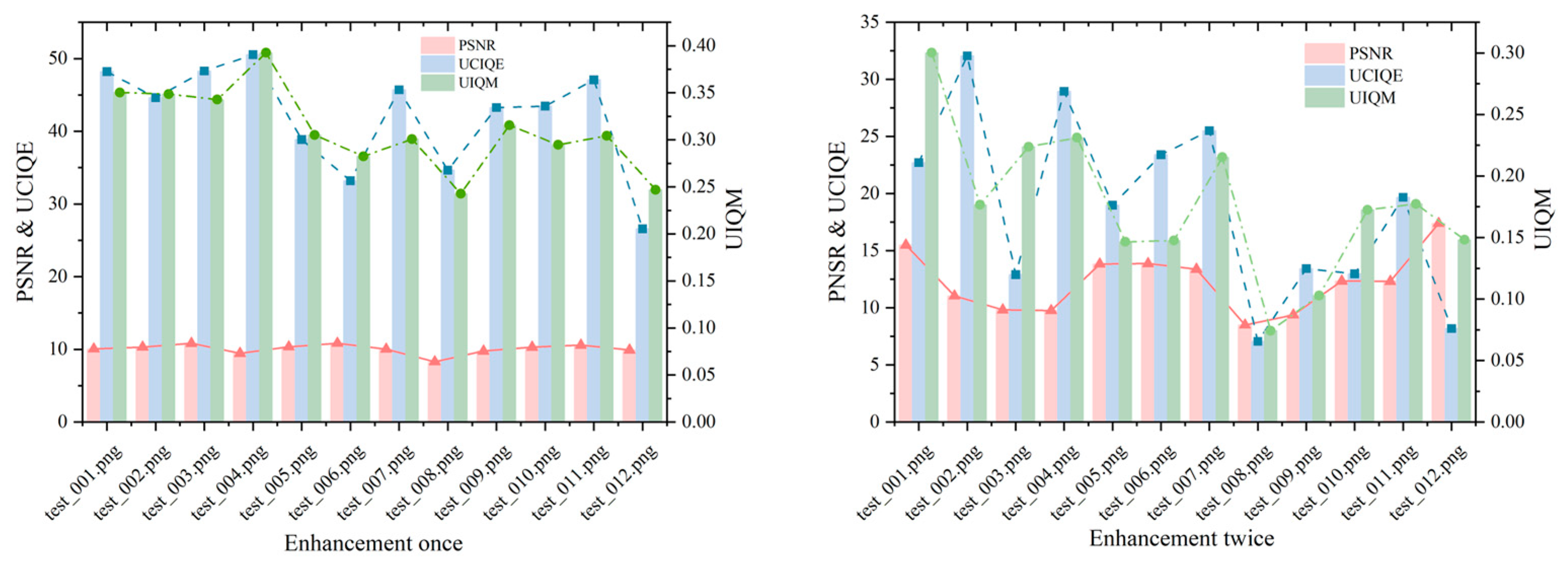
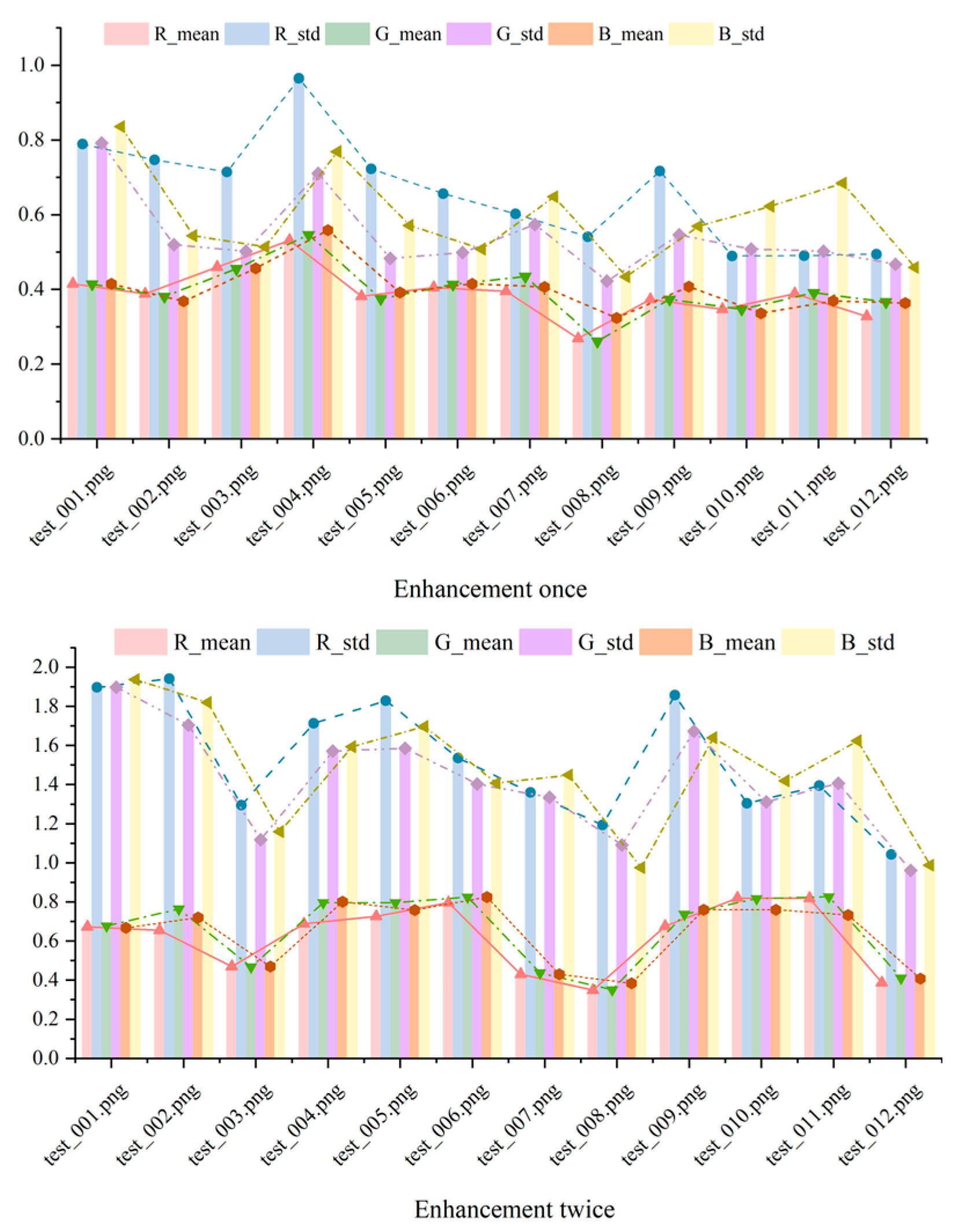
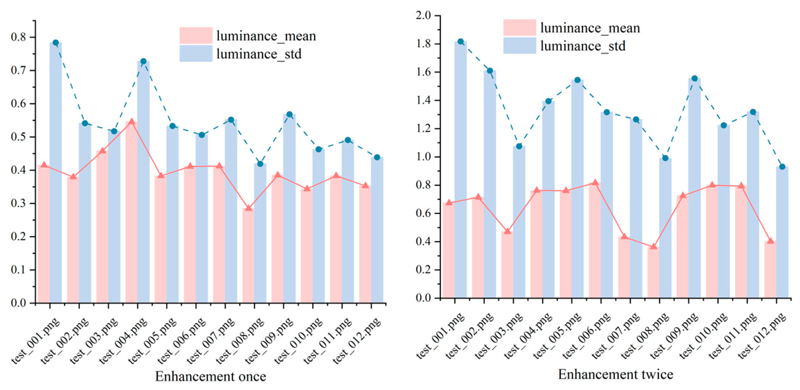
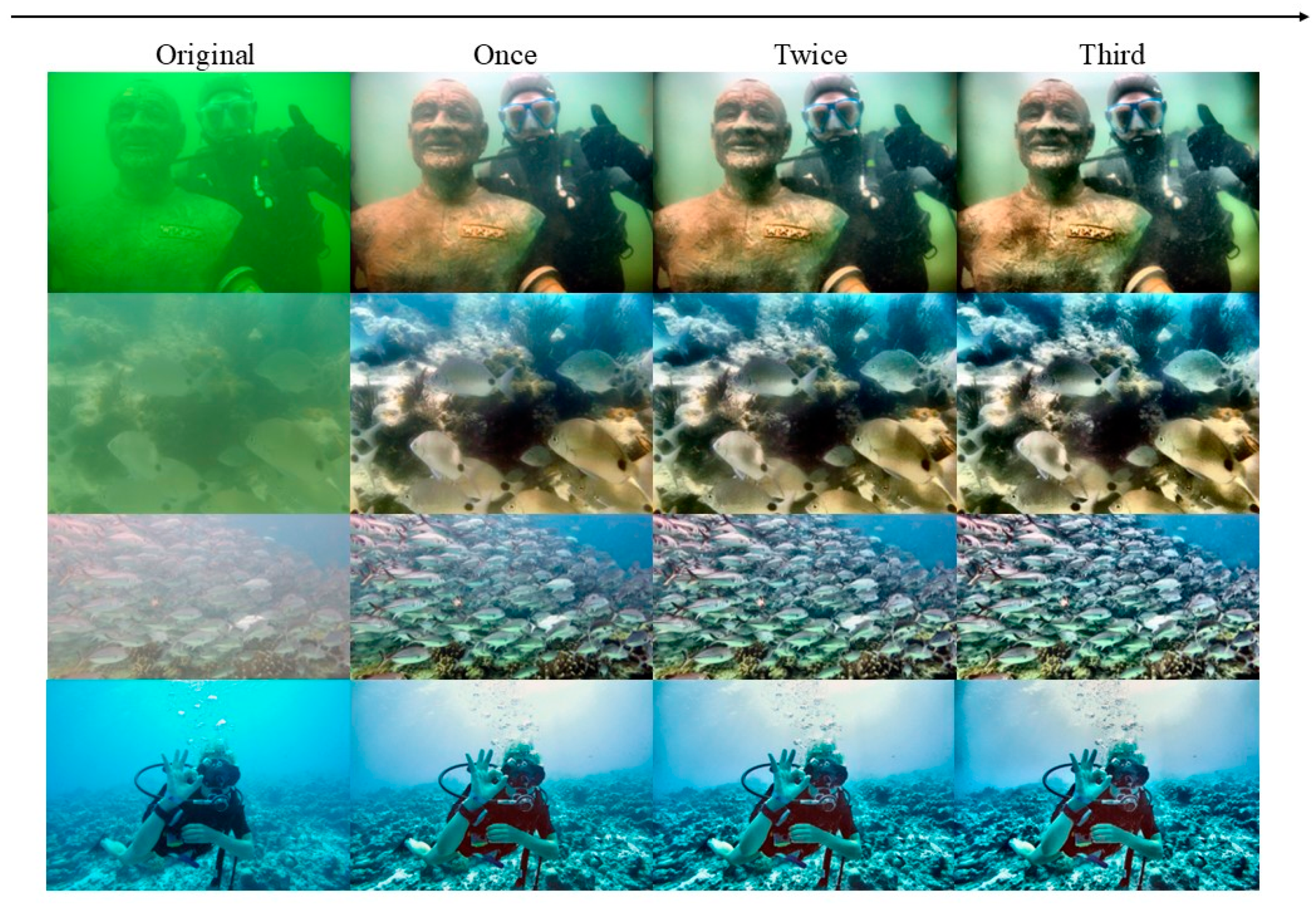


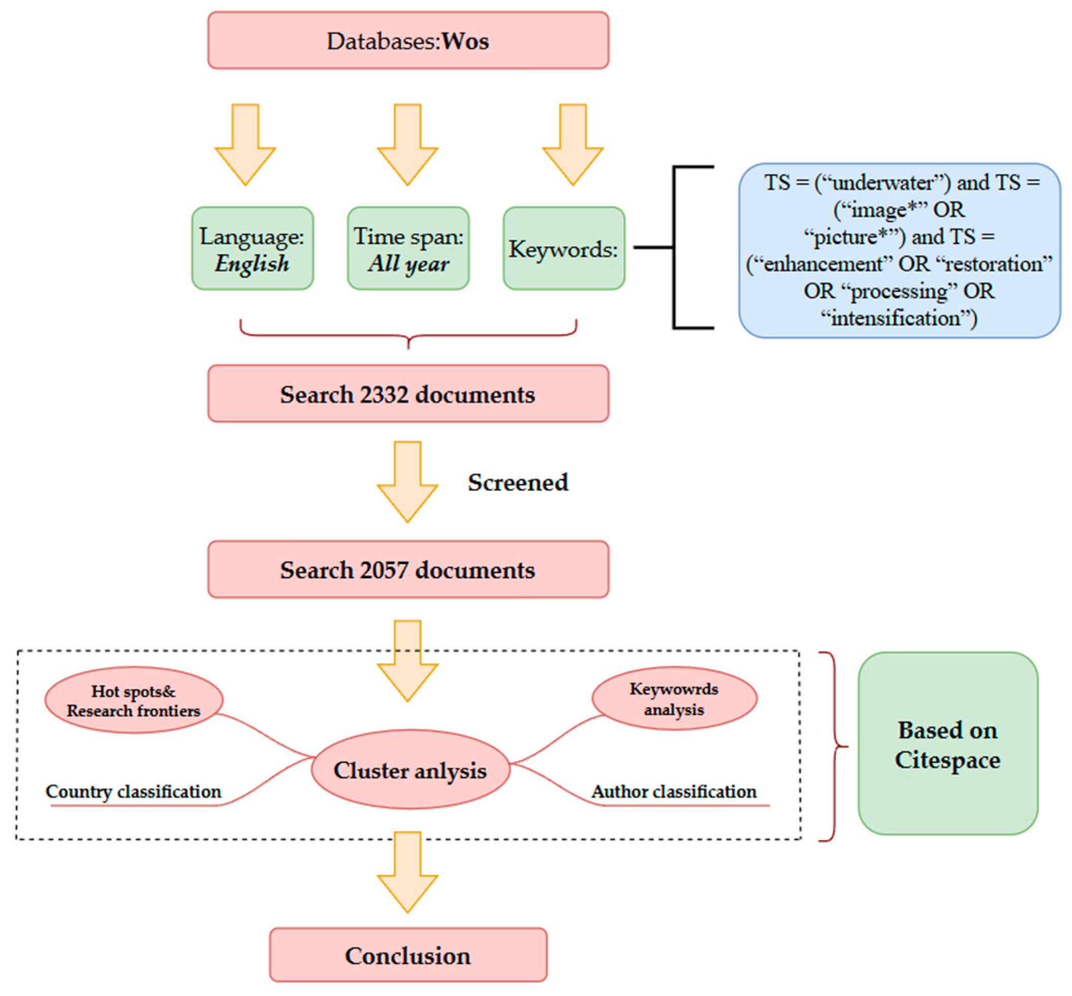
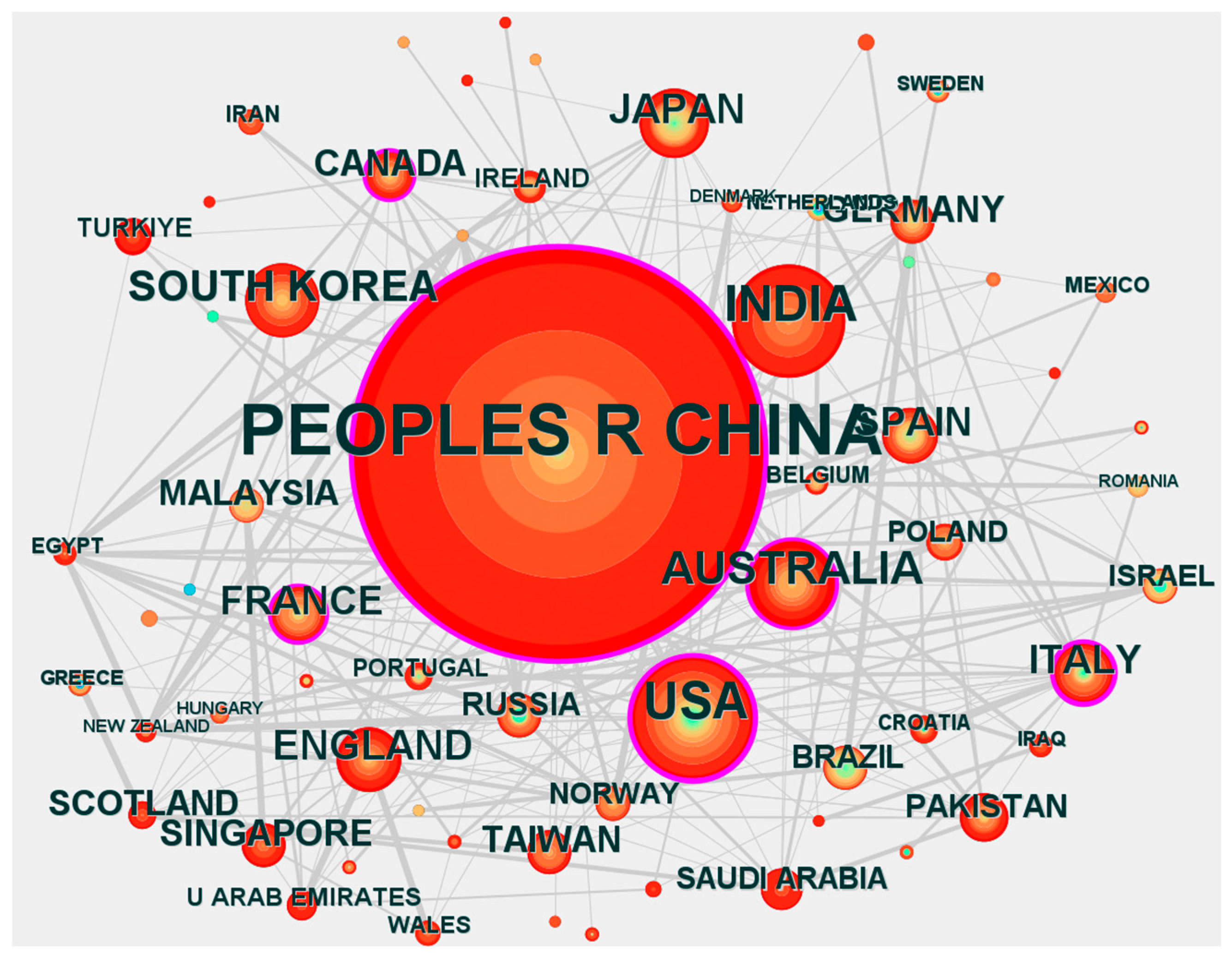
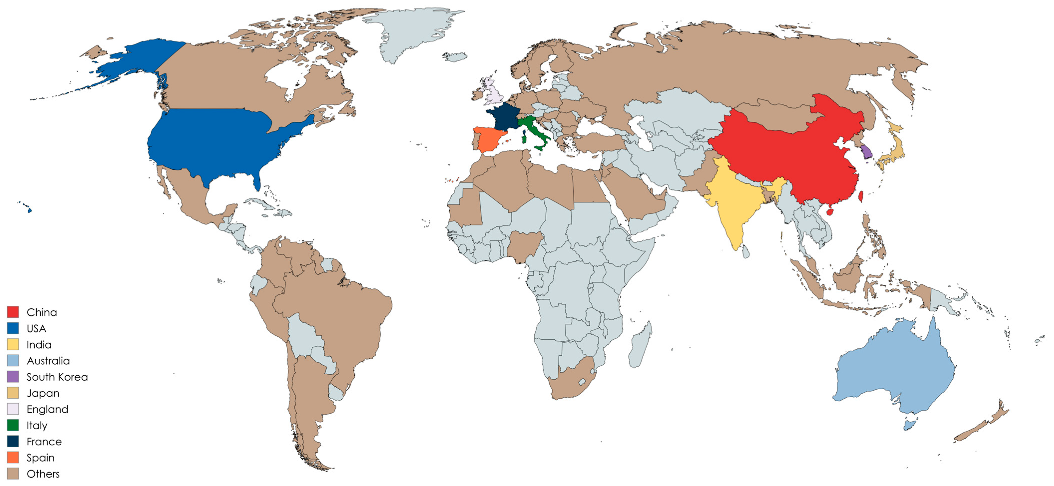

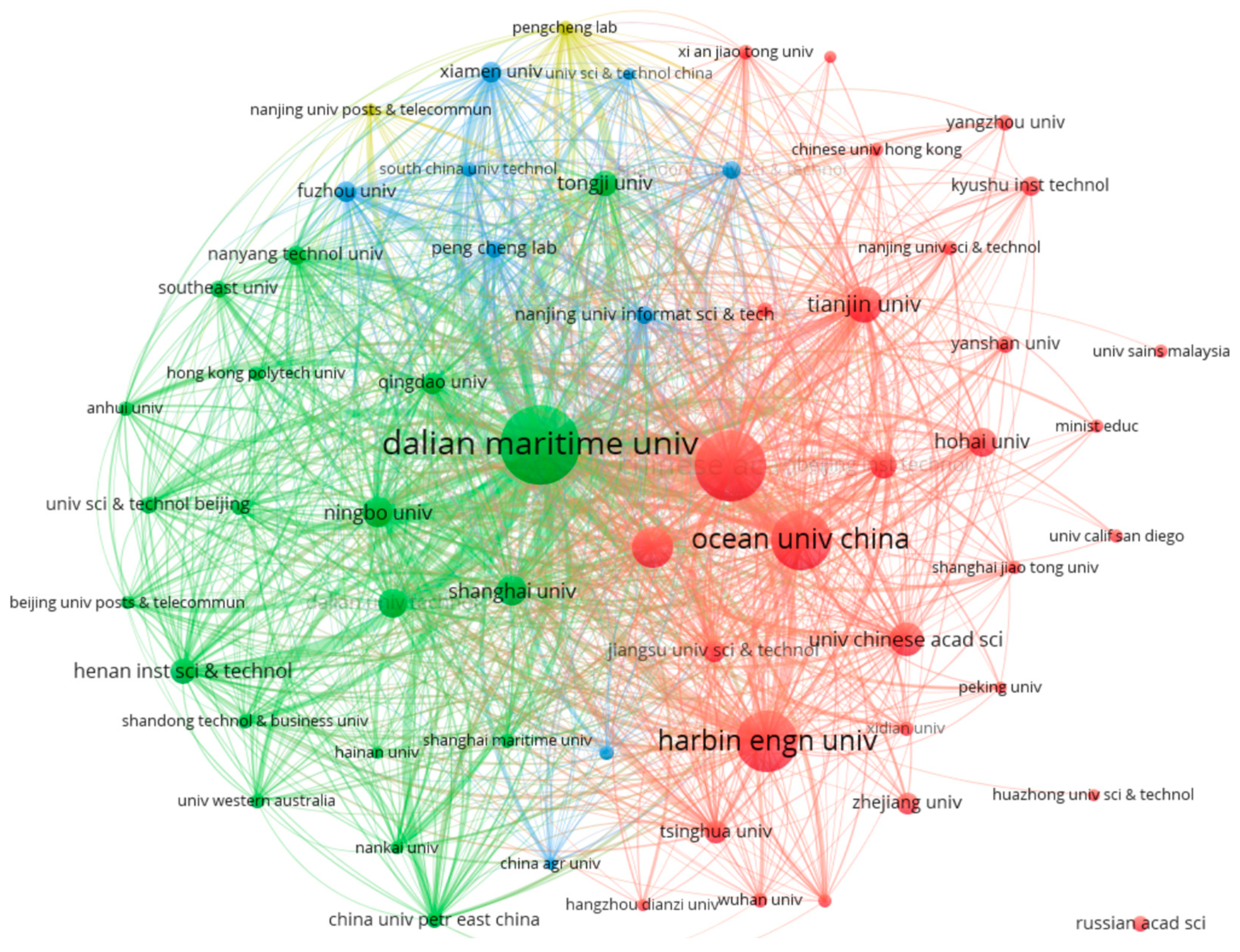
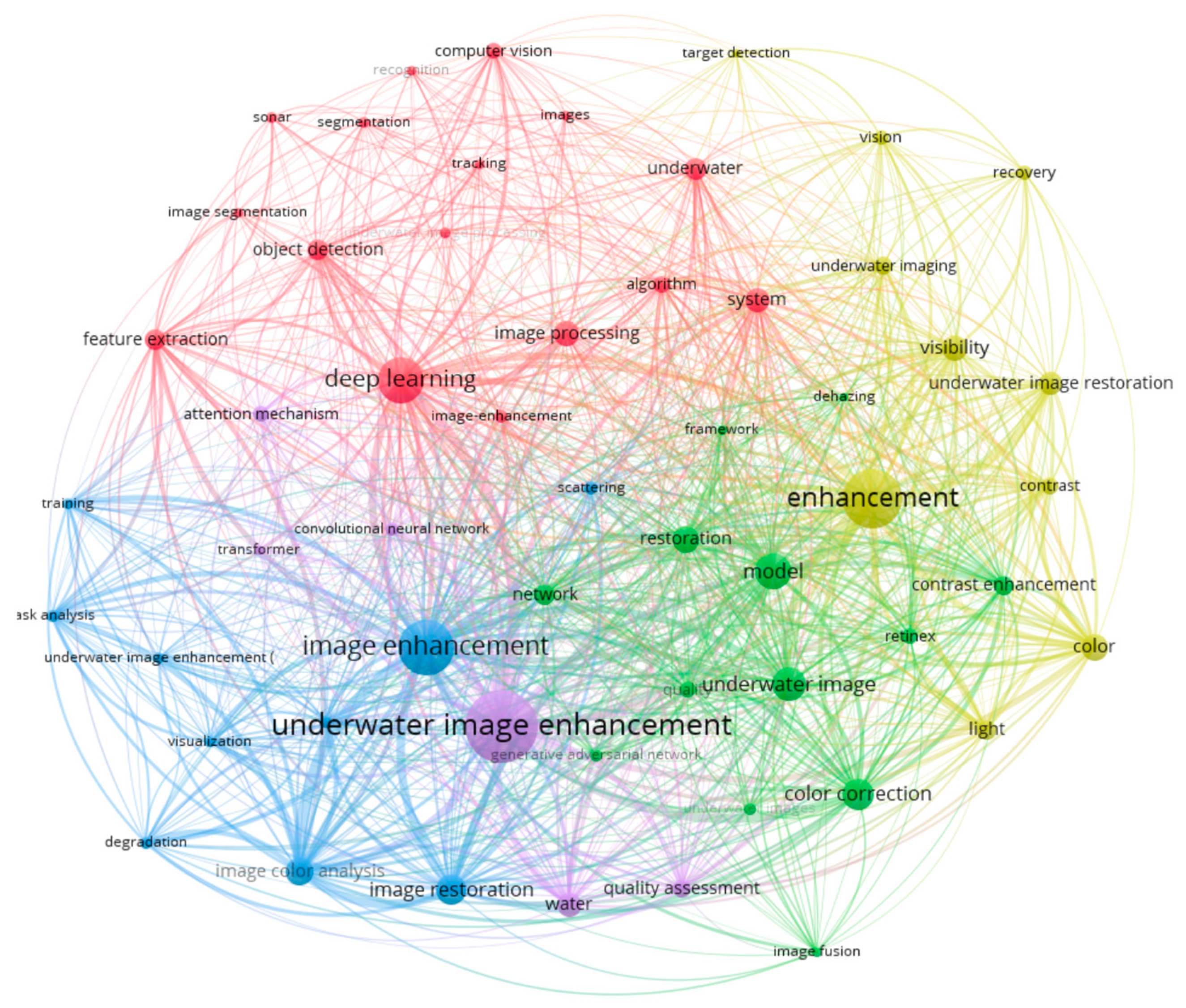
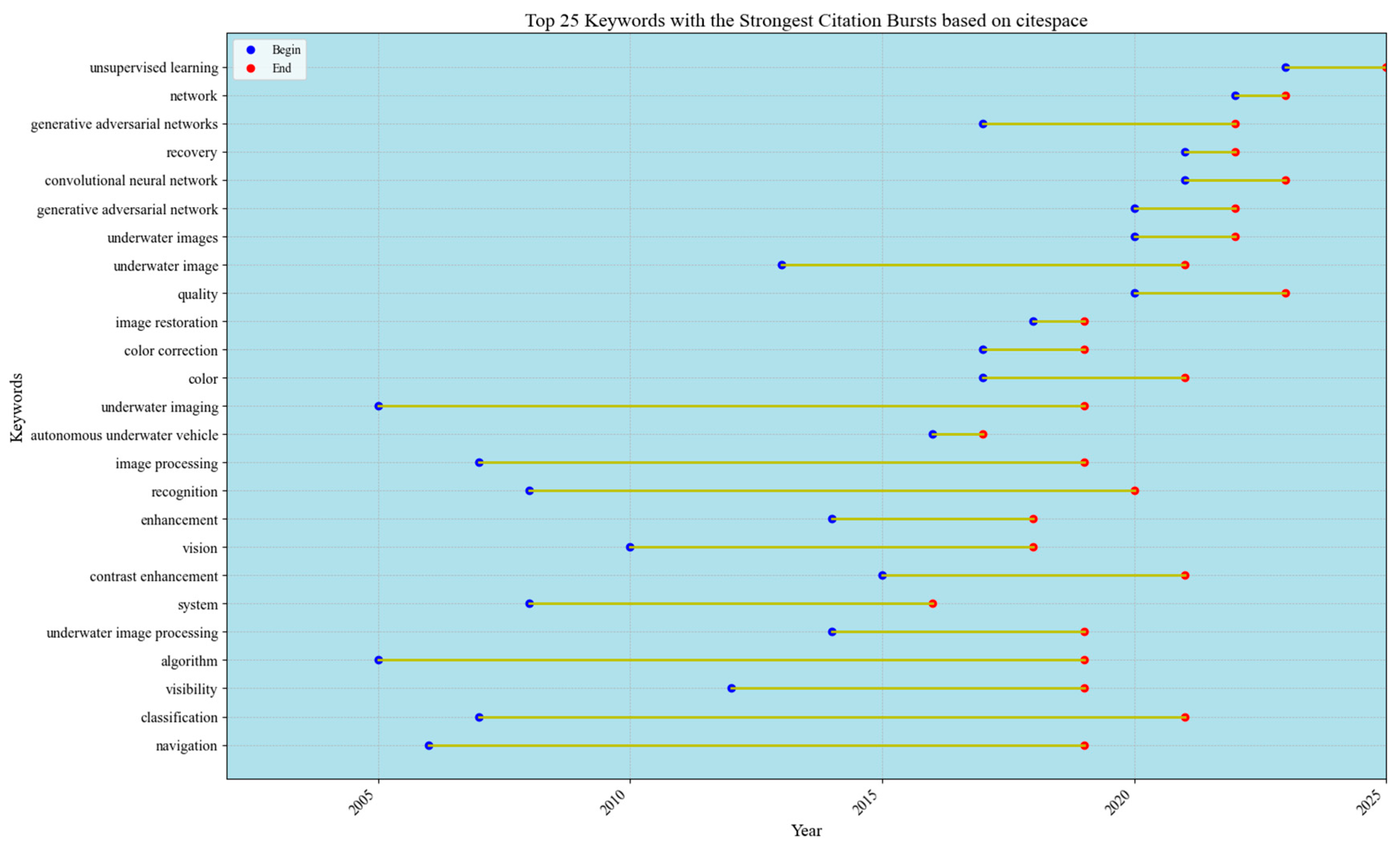
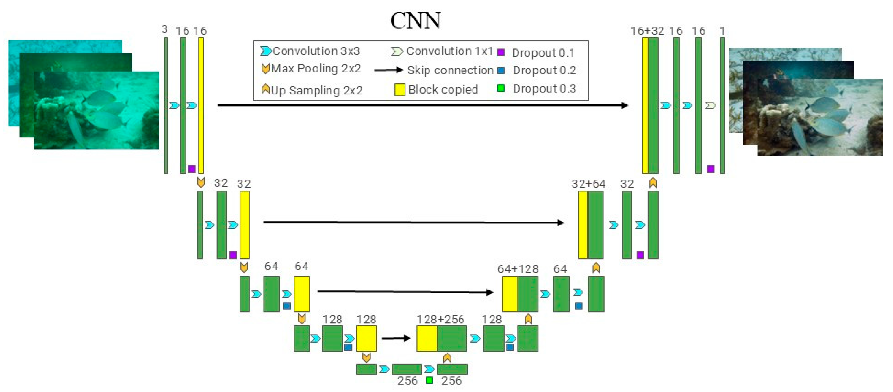
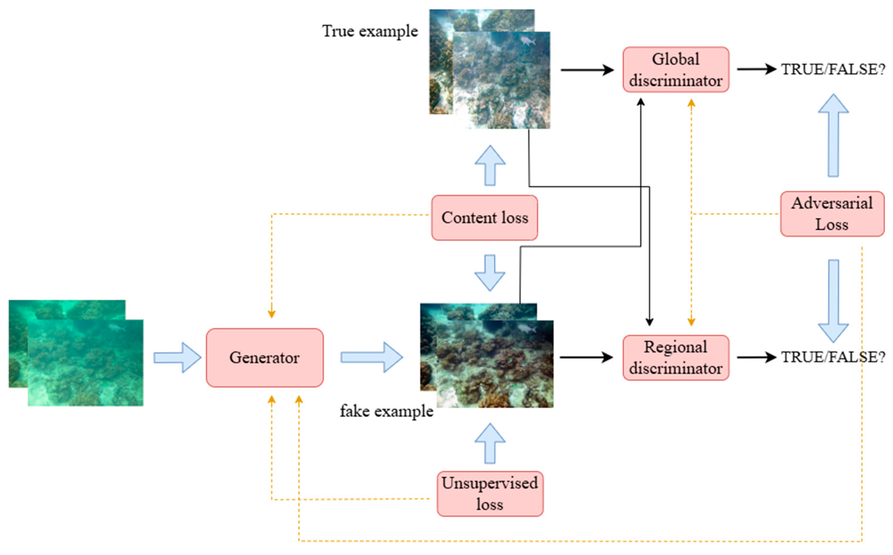
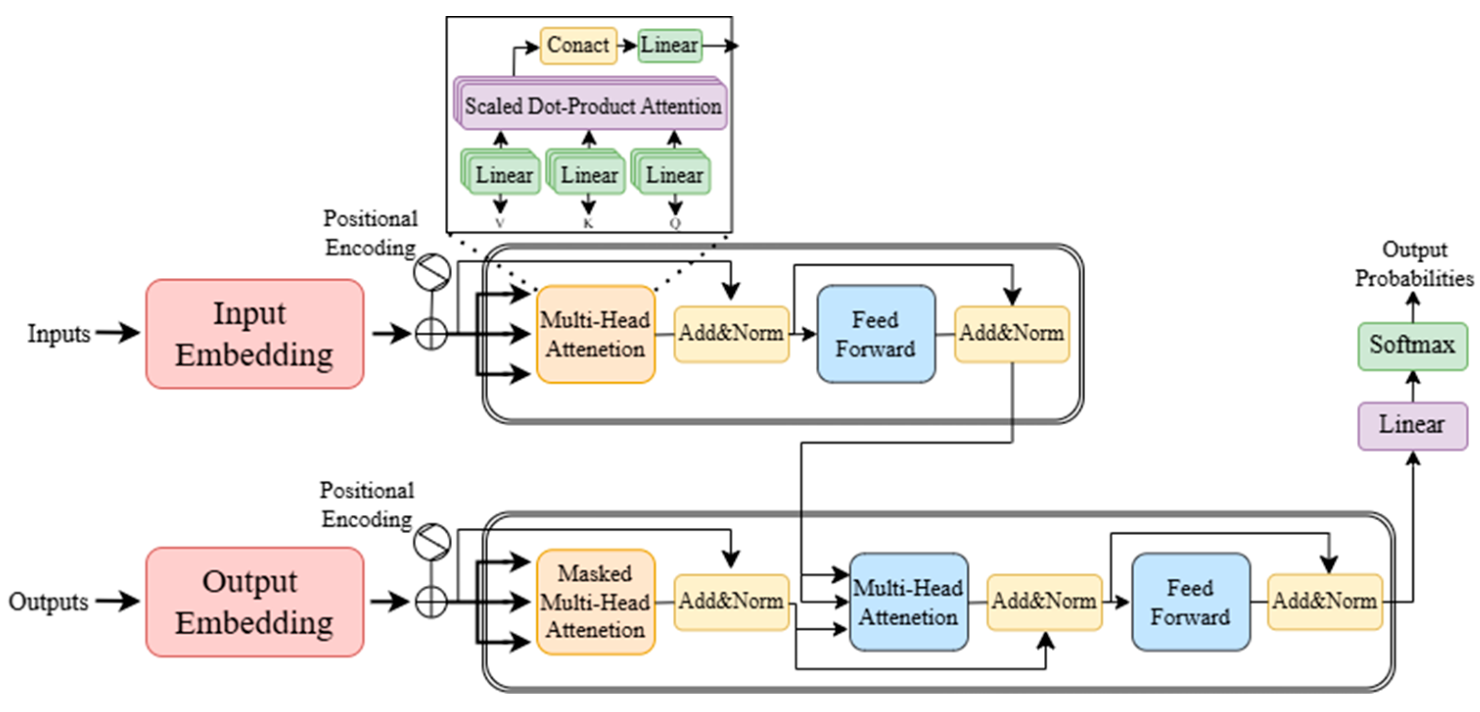
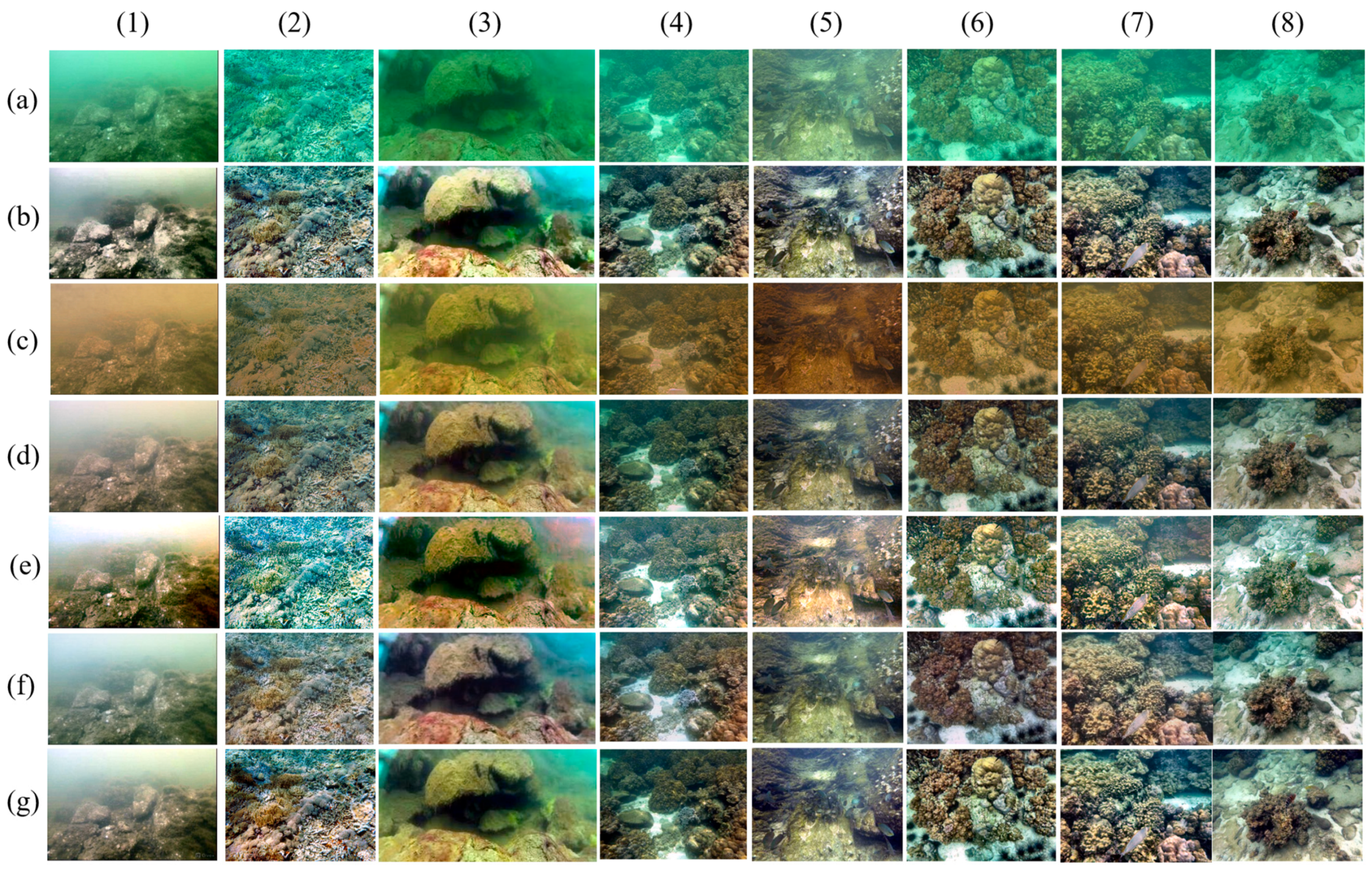
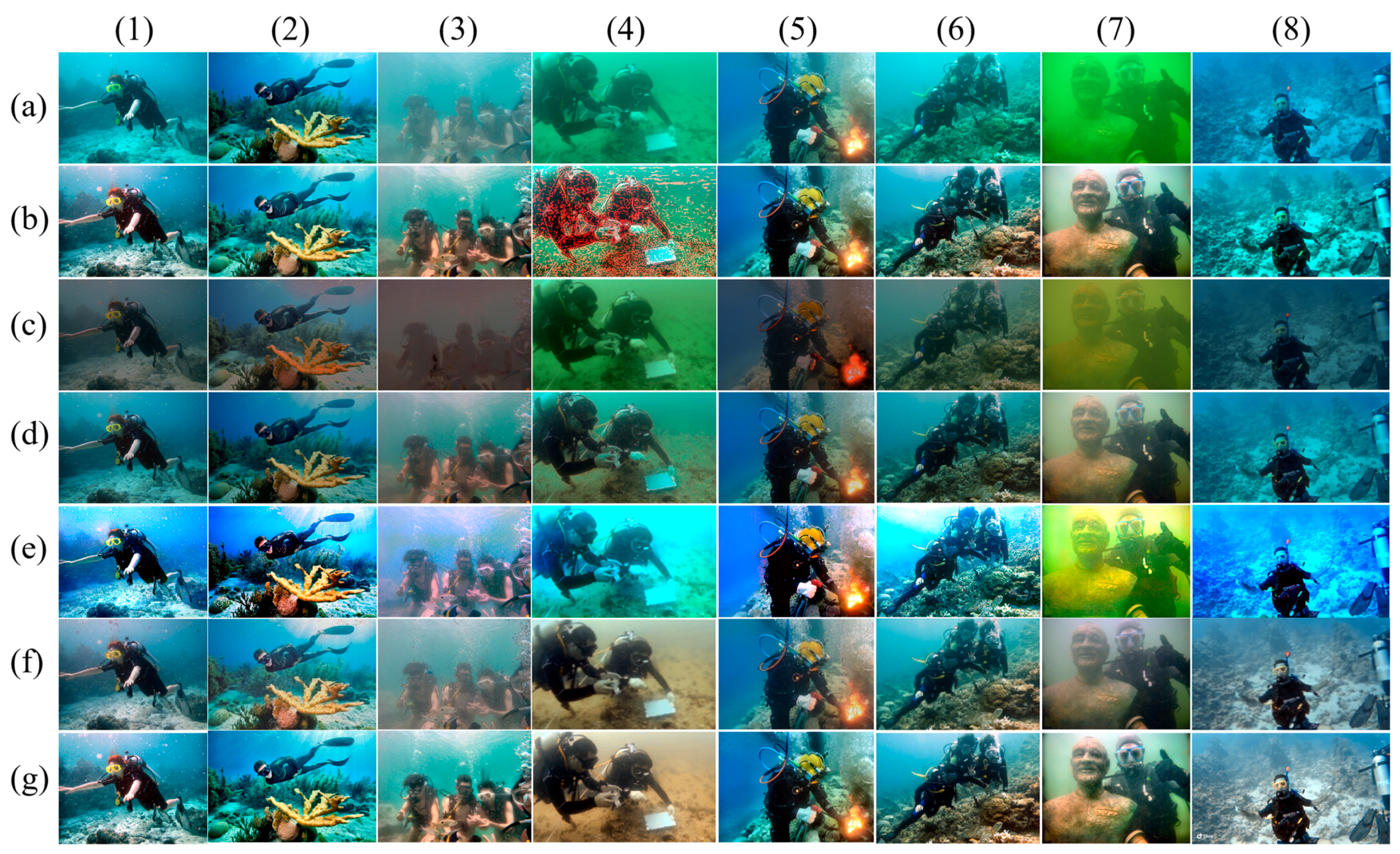
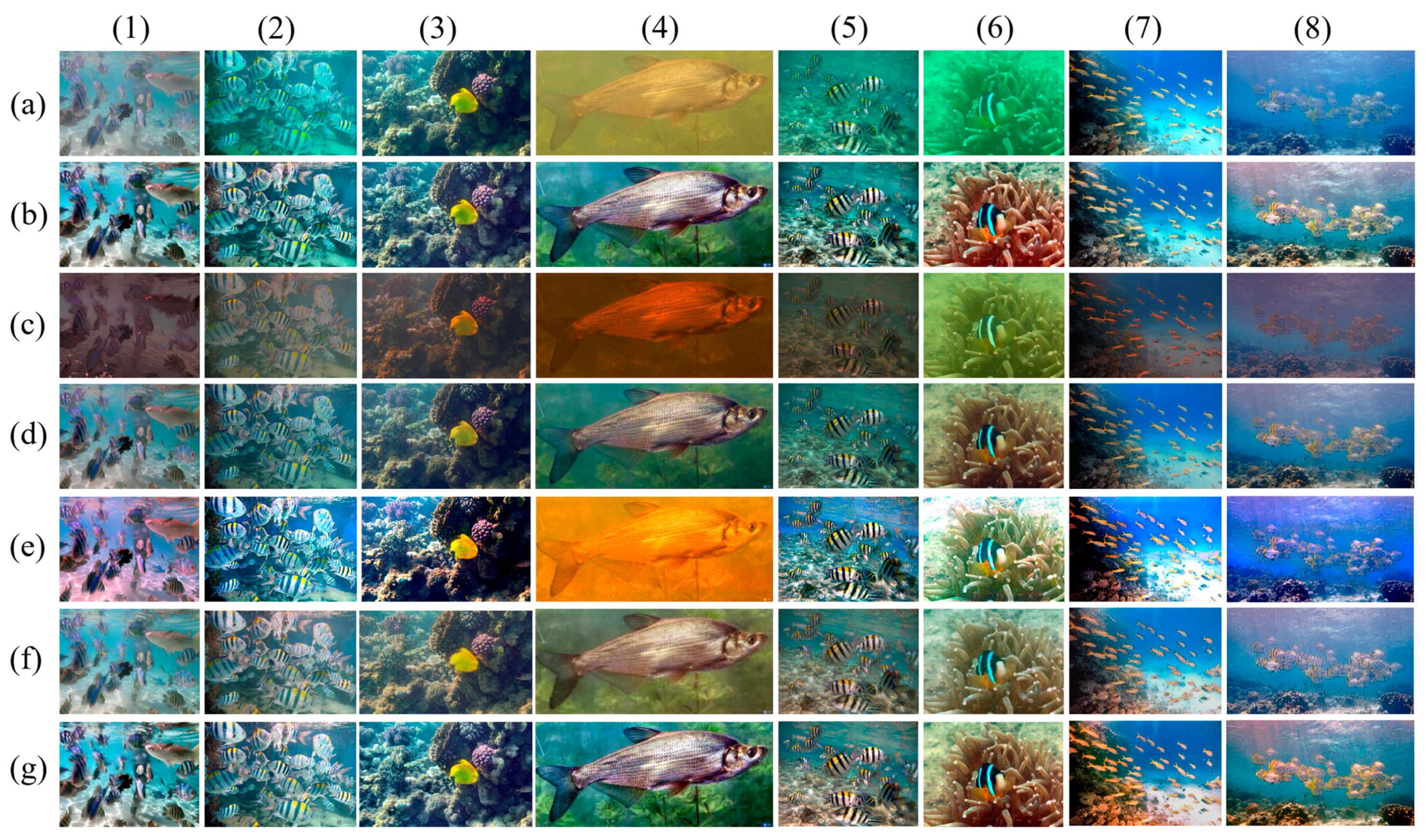
Disclaimer/Publisher’s Note: The statements, opinions and data contained in all publications are solely those of the individual author(s) and contributor(s) and not of MDPI and/or the editor(s). MDPI and/or the editor(s) disclaim responsibility for any injury to people or property resulting from any ideas, methods, instructions or products referred to in the content. |
© 2025 by the authors. Licensee MDPI, Basel, Switzerland. This article is an open access article distributed under the terms and conditions of the Creative Commons Attribution (CC BY) license (https://creativecommons.org/licenses/by/4.0/).