Stochastic and Nonlinear Dynamic Response of Drillstrings in Deepwater Riserless Casing Drilling Operation

Abstract

In order to gain an insight into the stress state of drillstring in riserless drilling conditions with Casing while Drilling (CwD) technology, a stochastic and nonlinear dynamic model of the drillstring under the excitation of the environmental load is established based on Hamilton principle and finite deformation theory. The distribution of tensile stress, bending stress, and effective stress along the axial direction of drillstring that is exposed to the ambient environment is emphasized, the influence of wall thickness and material of the drillpipe on the stress state of drillstring is also discussed. The numerical results show that significant fluctuations in cross-sectional stress occur during the riserless drilling process, particularly under varying hydrodynamic loads; the tensile stress and effective stress are larger on landing string and the maximum values of these stresses occur at the connection point of the landing string and casing string; the bending stress is larger on casing string and the maximum value occurs near the sea floor; and increasing the wall thickness and selecting the low-density material can help to reduce the stress of the drillstring. It can be concluded from the numerical results that during the CwD riserless drilling process, the effective stress on the cross section of drillstring is mainly determined by the tensile stress and the contribution of bending stress is comparably small, and the dangerous cross section of the drillstring is located at the connection point of landing string and casing string. The proposed dynamic model offers theoretical insights that can inform drillstring design and vibration mitigation strategies in CwD operations.

1. Introduction

Casing while Drilling (CwD), an innovative drilling technology that uses casing instead of conventional drill pipe to drill a well, is primarily proposed in order to drill and case a well simultaneously [1]. CwD is mainly used to eliminate the non-productive time (NPT) required to trip the drill pipe and run the casing. Field studies show that CwD can significantly enhance drilling efficiency and reduce the operational costs compared to the conventional drilling method. Additionally, it can be observed from field practices that the unique “plastering effect” of casing drilling can reduce drilling fluid loss, mitigate drilling induced formation contamination, enhance borehole stability, and increase the formation fracture pressure gradient [2,3,4,5]. Due to the advantages stated above, casing drilling technology has gradually been applied in formations where the wellbore instability problems and lost circulation events are prone to occur.

In recent years, the concept of deepwater riserless casing drilling technology has been proposed by drilling engineers. This technology is proposed to address the challenges of high daily operational costs, narrow safe mud weight window and frequent shallow geological hazards in deepwater drilling conditions [6,7,8]. Since CwD can handle the geological hazards resulting from shallow water and shallow gas and broaden the safe mud weight window of the shallow layer of the seabed, it allows for a deeper surface casing set depth compared with a conventional drilling method. This in turn reduces the number of casing strings required to meet well objectives, simplifies the wellbore structure, and significantly saves the drilling-related cost. Furthermore, a larger diameter wellbore will be guaranteed at the target formation, which will increase the oil drainage area and improve the production efficiency.

Although deepwater riserless casing drilling technology is highly promising for improving drilling efficiency and reducing operational costs, the technological breakthroughs in recent years have been limited due to the stringent requirements for specialized equipment. The equipment that is suitable for deepwater surface well drilling operations was first introduced by Nunzi et al. from Weatherford in 2010 [9]. This innovative system integrates conventional drill pipes at the top, serving primarily as running tools, with casing strings connected below. During riserless casing drilling operations, these conventional drill pipes lower the casing assembly onto the seabed and transmit torque and hook load from the derrick on the floating drilling platform. Throughout the drilling process, both the conventional drill pipe and casing strings remain directly exposed to seawater, subjecting them to complex external environmental loads, including combined wave and current load. However, it is crucial to note that conventional drill pipes and casing strings were primarily designed with considerations such as external collapse resistance, internal pressure resistance, and tensile strength, without explicitly accounting for the dynamic loads induced by deepwater marine environments. Due to the considerable length and large diameter-to-thickness ratio of the drilling assembly, significant deformation under environmental excitations can occur, resulting in complex dynamic behavior. Consequently, to ensure safe and efficient drilling operations, an in-depth analysis of the dynamic responses and stress states of the drill pipe-casing assembly under these complex environmental loading conditions is essential to provide valuable insights for enhancing structural integrity and optimizing equipment design specifically tailored for deepwater riserless casing drilling scenarios.

However important, few literatures have been reported to investigate the dynamic behavior and stress state of casing drilling assembly in both onshore and offshore working conditions. Dou et al. [10] investigated the whiling motion of casing drilling assembly in onshore inclined wellbore with both the energy method and laboratory experiments. The drilling assembly in this study is simplified as a shaft with pined-pined and fixed-pined ends. The effect of inclination angle, drillstring rotary speed, and flow rate of drilling fluid on the whirling motion of drilling assembly are examined. The model established in the above study neglects the effect of bit–rock interaction and the nonlinear deformation of the drillstring. Furthermore, this model can only be used to analyze the whirling motion of casing drilling assembly in onshore drilling conditions.

Currently, studies addressing drillstring dynamics during deepwater riserless drilling operations mainly focus on a conventional drill pipe. Graham et al. [11,12] conducted the first studies on drillstring vibration characteristics, focusing primarily on lateral free vibrations and dynamic responses under combined vessel surge motion and environmental loads. This study employed a simplified rigid–soft–rigid analytical model, ignoring bending stiffness in the intermediate section, rotational effects, bottom-hole pressure fluctuations, and nonlinear deformation effects, which significantly limited its scope. In subsequent research, Graham et al. [13] extended their analysis by including combined vessel surge and sway motions, observing that vessel motions predominantly affected bending stresses at the top of the drillstring, while stresses near the seabed were driven by environmental loads. Rheem et al. [14] studied the influence of drillstring rotation on vortex-induced vibrations using experimental and numerical methods, demonstrating that lateral vibration amplitudes peak when rotation frequencies approach natural frequencies. Samuel [15] employed an energy-based method to investigate vibration responses in highly inclined wells induced by fluctuations in bottom-hole pressure but excluded environmental loading. Obadina [16] analyzed the impacts of hydrodynamic loading and the Magnus effect on dual-wall drill pipe stresses, highlighting that substantial axial stress increases due to hydrodynamic forces. Su et al. [17] emphasized the effects of long-term vessel drift motions on drillstring dynamics, showing improved stress and deformation conditions with increased drillstring length below the mudline. Inoue et al. [18] numerically evaluated the Magnus effect caused by drillstring rotation, indicating significant increases in bending moments. Wada et al. [19] investigated longitudinal vibrations resulting from friction within heave compensation systems, emphasizing the necessity of real-time bottom-hole pressure monitoring. Chen et al. [20] established a three-dimensional nonlinear coupled dynamic model to investigate the influence of drillstring vibration on wellbore pressure in deepwater riserless drilling. The results indicate that lateral vibration predominantly induces peak pressure fluctuations, while torsional vibration governs the average pressure level, providing insight into the dynamic interaction between drillstring behavior and wellbore stability. Wang et al. [21] experimentally studied riserless rotating drillstring dynamics, revealing that rotation rate and current speed jointly affect vibration via nonlinear coupling of vortex-induced forces and Magnus effect.

Despite the comprehensive analyses in previous literature, detailed examinations of axial, bending, and effective stress distributions and their evolution over time in drillstrings during deepwater riserless casing drilling operations remain scarce. Moreover, past studies have not sufficiently identified the primary stress factors critical for drillstring structural safety, nor have they systematically explored the impact of modifying drillstring wall thickness and material properties under specific marine environmental conditions to prevent structural failures. To address these gaps, this study develops a three-dimensional finite element dynamic model incorporating longitudinal-transverse coupling effects for deepwater riserless casing drilling operations. It analyzes spatial and temporal distributions of axial, bending, and effective stresses along the drillstring, identifying the key stress factors impacting structural integrity. Additionally, the study investigates how variations in drillstring wall thickness and material properties influence stress distributions. The results from this research provide robust theoretical support for the structural strength design and optimization of drillstrings in deepwater riserless casing drilling scenarios.

2. Dynamic Model

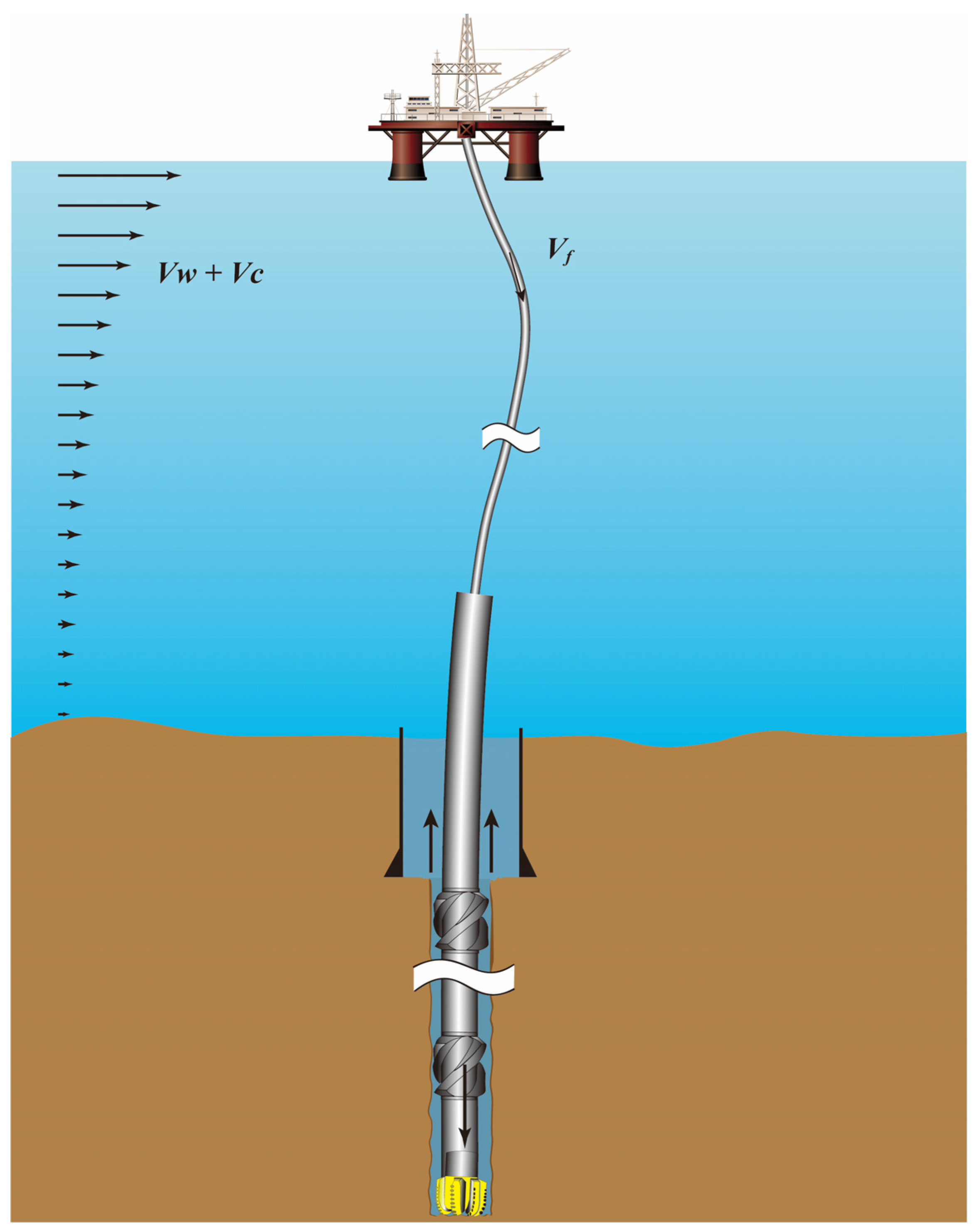
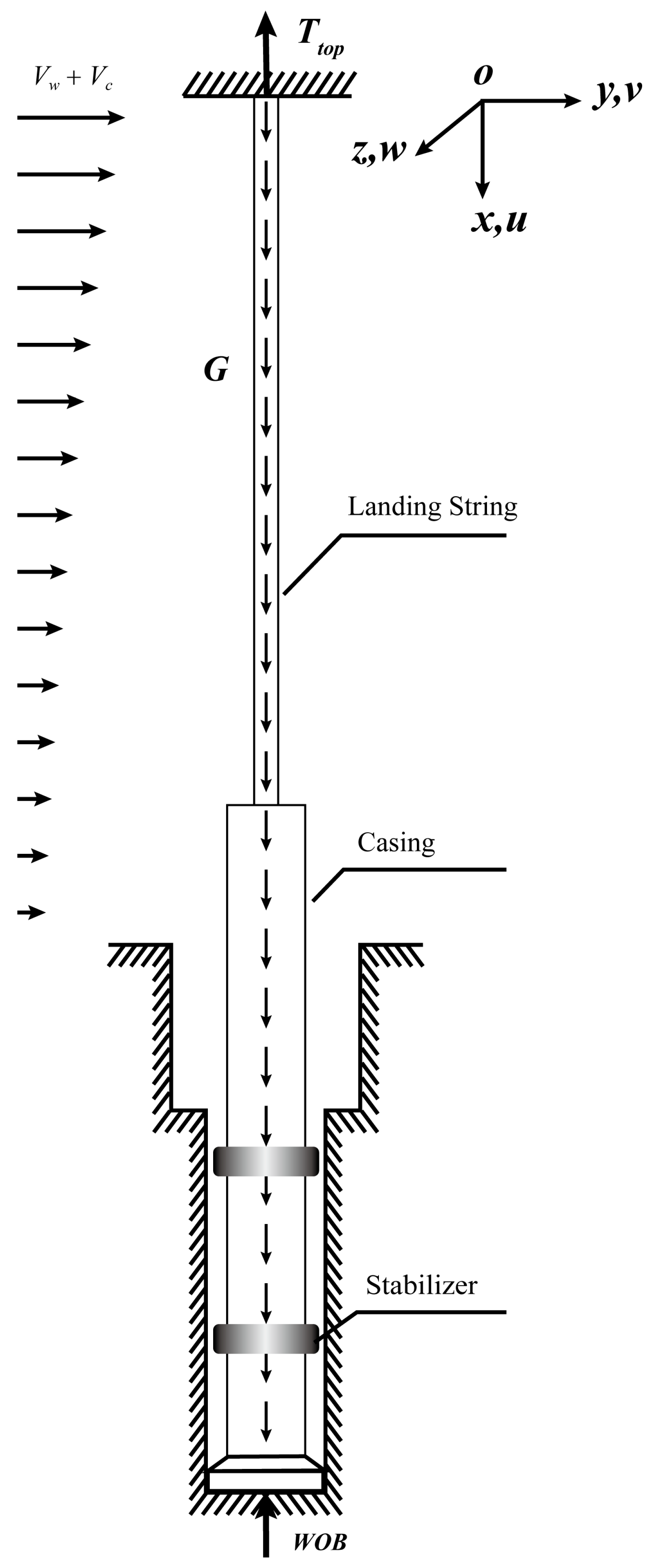
2.1. Problem Definitions

The schematic diagram of the casing drilling assembly that is proposed by Nunzi and used for deepwater surface casing drilling operation is shown in Figure 1 [9]. As illustrated, the surface casing strings are connected to conventional drill pipes via a casing adaptor, allowing the transmission of torque and hook load from the drilling platform to the casing assembly. This configuration allows the conventional drill pipe to serve both as a drilling tool and as a structural connector to the casing drilling assembly, thereby enabling the application of casing drilling technology in deepwater riserless drilling of the surface wellbore section.

The schematic diagram of the riserless casing drilling operation is shown in Figure 2. It can be seen from this figure that, during the drilling process, the casing strings instead of conventional drill pipes and bottom hole assembly are employed to drill a well. A drillable drill bit is installed at the bottom end of the casing strings to grind the formation and jet the drilling fluid. The top of the casing string is connected with a series of conventional drill pipes to transmit the torque and hook load from the derrick on the floating drilling platform. In Figure 2, the arrows inside and outside the drilling assembly indicate the flow of drilling fluid, with V_f denoting the corresponding flow velocity. The arrows on the left side of the drilling assembly represent the combined flow of ocean current and wave. Here, V_w denotes the flow velocity of wave particles, and V_c represents the flow velocity of the ocean current.

The dynamic model of the riserless casing drilling assembly is illustrated in Figure 3. In this model, the origin of the global Cartesian coordinate system is positioned at the connection point of the drill pipe and the floating drilling platform. The positive directions of the x- and y-axes are defined along the direction of gravity and the ocean current, respectively. The variable u, v and w represent the displacements of the drilling assembly along the x-, y-, and z-directions, respectively, in this coordinate system.

As illustrated in the figure, several key forces acting on the drilling assembly are labeled. T_top denotes the axial tension applied to the top of the drilling assembly by the hook on the drilling platform, represented by an upward-pointing arrow. G represents the gravitational force acting downward along the drillstring, indicated by a series of arrows directed downward along the axis of the assembly. At the bottom end, the weight-on-bit (WOB) corresponds to the reaction force exerted by the formation onto the drill bit, shown as an upward-pointing arrow. Additionally, the arrows on the left side of the drilling assembly represent the flow of water particles induced by the combined effects of ocean currents and wave motion. Collectively, these forces and associated displacements form the foundation for modeling the coupled dynamic behavior of the drillstring under deepwater drilling conditions.

Since torsional vibration is relatively insignificant in shallow seabed layers, it is excluded from the present model. Thus, only the dynamic response of the coupled axial-transverse vibration of the drilling assembly is considered in this study. The rotational speed of the drilling assembly is set as a constant value, which is consistent with on-site operation. For the convenient of analysis, some reasonable assumptions are made in this study regarding the structure, the material properties of the drilling assembly and some hydrodynamic considerations.

The assumptions are listed as follows:

(1)

The material of the drilling assembly is isotropic and homogeneous;

(2)

The drilling assembly stays in a linear elastic deformation state during the vibration process, and the material nonlinearity is neglected;

(3)

Only the damping from ambient seawater and drilling fluid is considered, the structural damping is neglected;

(4)

The cross section of the drilling assembly is always perpendicular to its axis during the deformation process;

(5)

The drill bit is in consistent contact with the formation, the stick-slip and bit bounce are neglected;

(6)

The rotational speed of the drilling assembly keeps constant during the drilling process, and the rotational vibration is neglected;

(7)

The horizontal velocity component of the wave particle is coincident with the flow direction of the current.

The initial stress and deformation state of the drilling assembly is set as the one in which only the gravitational force, hook load and WOB are applied on this assembly. According to the strain and displacement relationship at any point of the cross section along the axial direction of the drilling assembly, combined with the generalized Hamilton’s principle, the 3D nonlinear dynamic model of the drilling assembly considering the coupled effect of axial and transverse deformation during the deepwater riserless casing drilling process can be derived.

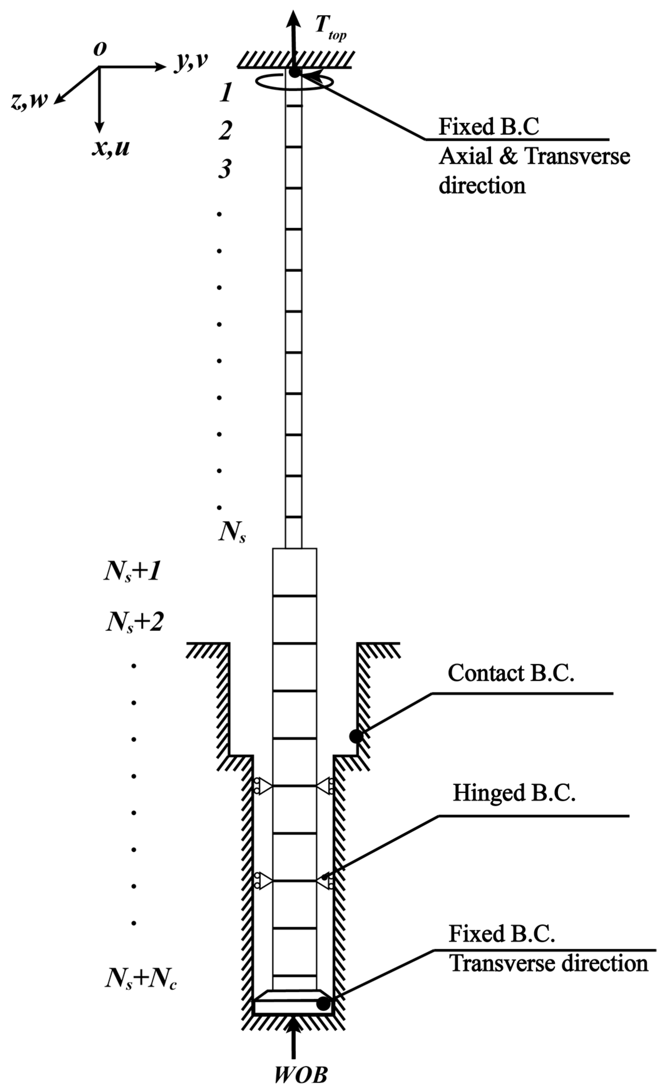
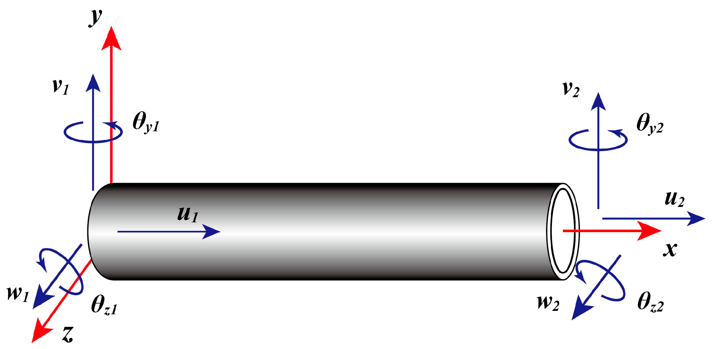
2.2. Finite Element Model

For the finite element analysis of structural dynamics, the entire structure should first be discretized into a series of elements. For each element, the mass matrix, stiffness matrix, damping matrix, and force vector are derived using energy-based methods. These elemental matrices and vectors are then assembled according to the connectivity of the drillstring elements to formulate the global finite element equation of motion for the entire structure. The finite element model of deepwater riserless casing drilling assembly is shown in Figure 4.

Figure 4 illustrates the discretization scheme and boundary conditions of the finite element model. In this study, the drilling assembly is discretized using Euler–Bernoulli beam elements along the positive direction of the x-axis, from the top of the landing string to the drill bit. The numbers 1 to N_s + N_c represent the sequential element numbering in the finite element model, where N_s and N_c denote the number of elements in the landing string and casing, respectively. The top of the drilling assembly is rigidly connected to the rotary table during operation, and thus is modeled with fixed boundary conditions in both the axial and transverse directions. Stabilizers, which are placed at designated locations along the casing section, serve to centralize the assembly within the wellbore. Given their diameter closely matches that of the wellbore, the corresponding element nodes are restricted in the transverse direction, while remaining free to move axially and rotate—thus a hinged boundary condition is applied transversely. At the drill bit, whose diameter is approximately equal to the wellbore diameter and which is restrained against rotation, a fixed boundary condition is imposed in the transverse direction. Additionally, during the drilling process, once the transverse displacement of any node exceeds the radial clearance between the drill pipe and the borehole wall, contact is assumed to occur. In such cases, a reaction force is applied by the borehole wall to the drillstring node. To account for this interaction, a contact boundary condition is introduced for the section of the drilling assembly below the mud line.

To derive the finite element dynamic governing equations within the framework stated above, the generalized Hamilton’s principle, which extends classical Hamiltonian mechanics to non-conservative systems, is applied. This approach is particularly effective for complex coupled dynamic systems, such as the drill string in the drilling fluid-filled wellbore, where energy dissipation and external work (e.g., damping, wave excitation) must be considered systematically. It ensures a consistent formulation when dealing with multiple degrees of freedom and boundary interactions. [22], that is:

$${\displaystyle {\int }_{t_1}^{t_2}\left(\delta T-\delta U\right)dt}+{\displaystyle {\int }_{t_1}^{t_2}\delta W}dt=0$$

(1)

where, $\delta T$ and $\delta U$ are the variation in kinetic and potential energy of the whole dynamic system, and $\delta W$ is the virtual work conducted by an external load.

2.2.1. Kinetic Energy

The kinetic energy of an infinitesimal tubular element of the dynamic system includes both the rotational kinetic energy and translational kinetic energy. For an infinitesimal tubular element, the kinetic energy can be derived by differentiating the position vector of any point on the cross section of the deformed drilling assembly with respect to time, multiplying the material density and integrating over the volume of the element. After the above manipulation, the kinetic energy can be expressed as follows:

$$T_e={\displaystyle \frac{1}{2}}{\displaystyle {\int }_{x_e}^{x_e+L_e}\left\{\rho A{V}_G^2+J_1{\omega }_1^2+J_2{\omega }_2^2+\left(J_1+J_2\right){\omega }_3^2\right\}dz}$$

(2)

where, x_e represents the location of the tubular element along the axial direction of the drilling assembly, m; L_e represents the tubular element length, m; $\rho$ represents the material density, kg/m³; A represents the cross sectional area, m²; V_G represents the translational velocity of the centroid of tubular element, m/s; J₁ and J₂ represent the mass moment inertia of the tubular element with respect to the y axis and z axis, respectively, kg·m²; and ${\omega }_i$ represents the angular velocity of cross section of the tubular element with respect to the x, y and z axis of global coordinate, rad/s;

The translational velocity of the centroid of tubular element can be expressed as:

$${\overrightarrow{V}}_G=\dot{u}\overrightarrow{i}+\dot{v}\overrightarrow{j}+\dot{w}\overrightarrow{k}$$

(3)

where, u, v and w represent the displacement of the tubular element centroid in the x, y and z directions, m; and $\overrightarrow{i}$, $\overrightarrow{j}$ and $\overrightarrow{k}$ represent the unit vector in the x, y and z axis.

Since the cross section of the tubular element is central symmetry, the mass moment inertia of the cross section of the tubular element with respect to the y axis and z axis are same and can be expressed as:

$$J_2=J_3=\rho I$$

(4)

where, I represent the moment inertia of the cross section with respect to y axis and z axis respectively.

During the vibration process, the angular velocity of any point on the cross section of the tubular element with respect to the x, y and z axis are as follows:

$$\{\begin{array}{l}{\omega }_1=-\dot{\alpha }\cos \phi \sin \psi +\dot{\phi }\cos \psi \\ {\omega }_2=\dot{\alpha }\sin \phi +\dot{\psi }\\ {\omega }_3=\dot{\alpha }\cos \phi \cos \psi +\dot{\phi }\sin \psi \end{array}$$

(5)

where, $\phi$ and $\psi$ represents the rotational angle of the cross section of tubular element with respect to y and z axis, respectively; α represents the angular velocity of any point on the cross section of the tubular element with respect to the z axis, rad/s. Since the torsional deformation of drilling assembly is not considered in this study, thus:

$$\dot{\alpha }=\mathsf{\Omega }=const$$

(6)

During the vibration process, the rotational angle of the cross section with respect to the y and z axis is comparably small (less than 10 degree). According to small rotational angle assumption, the angular velocity can be simplified as follows:

$$\{\begin{array}{c}{\omega }_1=-\mathsf{\Omega }\psi +\dot{\phi }\\ {\omega }_2=\mathsf{\Omega }\phi +\dot{\psi }\\ {\omega }_3=\mathsf{\Omega }+\dot{\phi }\psi \end{array}$$

(7)

Substituting Equations (3) and (7) into Equation (2) gives the expression of the kinetic energy of an infinitesimal tubular element along the drilling assembly:

$$\begin{array}{ll}{T}_e& ={\displaystyle \frac{1}{2}}{\rho }_s{A}_e{\displaystyle {\int }_{x_e}^{x_e+L_e}\left({\dot{u}}^2+{\dot{v}}^2+{\dot{w}}^2\right)}dx\\ & +{\displaystyle \frac{1}{2}}{\displaystyle {\int }_{x_e}^{x_e+L_e}\left(J_1({\dot{v}}^{\prime }-\mathsf{\Omega }{w}^{\prime }{)}^2+J_2({\dot{w}}^{\prime }+\mathsf{\Omega }{v}^{\prime }{)}^2+\left(J_1+J_2\right)(\mathsf{\Omega }+{\dot{w}}^{\prime }{v}^{\prime }{)}^2\right)}dx\end{array}$$

(8)

2.2.2. Potential Energy

Since the motion of the dynamic system is induced by both the rigid body rotation and elastic deformation, the finite strain beam theory in fixed frame is used. The finite strain beam theory is based on finite strain measures which is geometrically exact and can be used to capture axial strain and curvature of the dynamic system.

Using the expressions of Green’s strain and second Kirchhoff stress, neglecting the Poisson’s effect, the expression of strain potential energy for any infinitesimal tubular element can be expressed as follows [23]:

$$\begin{array}{ll}{U}_e& ={\displaystyle \frac{1}{2}}{\displaystyle {\int }_{V_e}{\sigma }_{ij}{\epsilon }_{ij}d{V}_0}\\ & ={\displaystyle \frac{1}{2}}{\displaystyle {\int }_{x_e}^{x_e+L_e}\left\{EI\left[{\left(v^{″}\right)}^2+{\left(w^{″}\right)}^2\right]+EA{\left[u^{\prime }+\frac{1}{2}{\left(v^{\prime }\right)}^2+\frac{1}{2}{\left(w^{\prime }\right)}^2\right]}^2\right\}dx}\end{array}$$

(9)

where, E represents the elastic modulus of tubular element, Pa; A represents the cross-sectional area, m².

2.2.3. Virtual Work by Flowing Drilling Fluid

During the drilling process, the drilling fluid is mainly used to circulate in the wellbore to bring the drill cuttings from the bottom of the well to the ground, cool the drill bit and balance the formation pressure to stabilize the wellbore. It has been studied by several researchers that, the flowing drilling fluid will affect the dynamic behavior of the drilling assembly. The effect of drilling fluid on the dynamics of drilling assembly mainly includes the following aspects [24]:

(1)

The inviscid fluid dynamic force and hydrostatic force of the flowing drilling fluid inside the drilling assembly;

(2)

The inviscid fluid dynamic force, viscous force and hydrostatic force of the flowing drilling fluid in the annulus between drilling assembly and wellbore wall;

(3)

The frictional force of flowing drilling fluid from both inside and outside of the drilling assembly.

The inviscid fluid dynamic force and hydrostatic force exerted by the inside flowing drilling fluid in the transversal direction can be expressed as follows:

$$F_{in}=-M_f{\left({\displaystyle \frac{\partial }{\partial t}}+U_i{\displaystyle \frac{\partial }{\partial x}}\right)}^2\left(v\overrightarrow{j}+w\overrightarrow{k}\right)-A_f{\displaystyle \frac{\partial }{\partial x}}\left(p_i{\displaystyle \frac{\partial }{\partial x}}\right)\left(v\overrightarrow{j}+w\overrightarrow{k}\right)$$

(10)

where, M_f represents the mass per unit length of the drilling fluid inside the drilling assembly, kg/m; U_i represents the flow velocity of inside drilling fluid, m/s; A_f represents the inner cross-sectional area of the drilling assembly, m²; and P_i represents the pressure inside the drilling assembly, Pa.

The inviscid fluid dynamic force and hydrostatic force exerted by the outside drilling fluid in transversal direction can be expressed as follows:

$$F_{out}=-\chi {\rho }_f{A}_o{\left({\displaystyle \frac{\partial }{\partial t}}-U_o{\displaystyle \frac{\partial }{\partial x}}\right)}^2\left(v\overrightarrow{j}+w\overrightarrow{k}\right)+A_o{\displaystyle \frac{\partial }{\partial x}}\left(p_o{\displaystyle \frac{\partial }{\partial x}}\right)\left(v\overrightarrow{j}+w\overrightarrow{k}\right)$$

(11)

where, ${\rho }_f$ represents the density of the drilling fluid, kg/m³; A_o represents the outside cross-sectional area of the drilling assembly, m²; U_o represents the flow velocity of outside drilling fluid, m/s; P_o represents the outside pressure, Pa; and χ represents the added mass coefficient, which is dimensionless. The added mass coefficient is mainly used to take into account the effect of drilling fluid that adhere to the surface of the tubular element during the vibration process. The expression of the added mass coefficient can be expressed as follows [25]:

$$\chi ={\displaystyle \frac{{\left(D_a/D_o\right)}^2+1}{{\left(D_a/D_o\right)}^2-1}}$$

(12)

where, D_a represents the diameter of wellbore, m; D_o represents the outside dimeter of drilling assembly, m.

The viscous force exerted by the outside drilling fluid on the tubular element can be expressed as follows:

$$F_N=-{\displaystyle \frac{1}{2}}{C}_f{\rho }_f{D}_o{U}_o\left({\displaystyle \frac{\partial }{\partial t}}-U_o{\displaystyle \frac{\partial }{\partial x}}\right)\left(v\overrightarrow{j}+w\overrightarrow{k}\right)-k{\displaystyle \frac{\partial }{\partial t}}\left(v\overrightarrow{j}+w\overrightarrow{k}\right)$$

(13)

where, C_f and k represent the viscous damping coefficients. C_f is a semi-empirical coefficient. Usually, 0.0125 [26] is adopted. K is mainly determined by the dynamic viscosity, Reynolds number and Strouhal number of drilling fluid [26].

The tangential frictional force that is exerted by both the inside and outside drilling fluid can be expressed as follows:

$$F_f=M_{f}g-A_f{\displaystyle \frac{\partial p_i}{\partial x}}-{\displaystyle \frac{1}{2}}{C}_f{\rho }_f{D}_o{U}_o^2$$

(14)

Thus, during the drilling process, the virtual work that act on the tubular element and is achieved by inside and outside flowing drilling fluid can be expressed as follows:

$$\{\begin{array}{c}\delta W_{Fx}={\displaystyle {\int }_{x_e}^{x_e+L_e}{F}_x\cdot \delta udx}\\ \delta W_{Fy}={\displaystyle {\int }_{x_e}^{x_e+L_e}{F}_y\cdot \delta vdx}\\ \delta W_{Fz}={\displaystyle {\int }_{x_e}^{x_e+L_e}{F}_z\cdot \delta wdx}\end{array}$$

(15)

where, F_x, F_y and F_z represent the forces that act on tubular element by the inside and outside flowing drilling fluid in x, y and z directions, respectively.

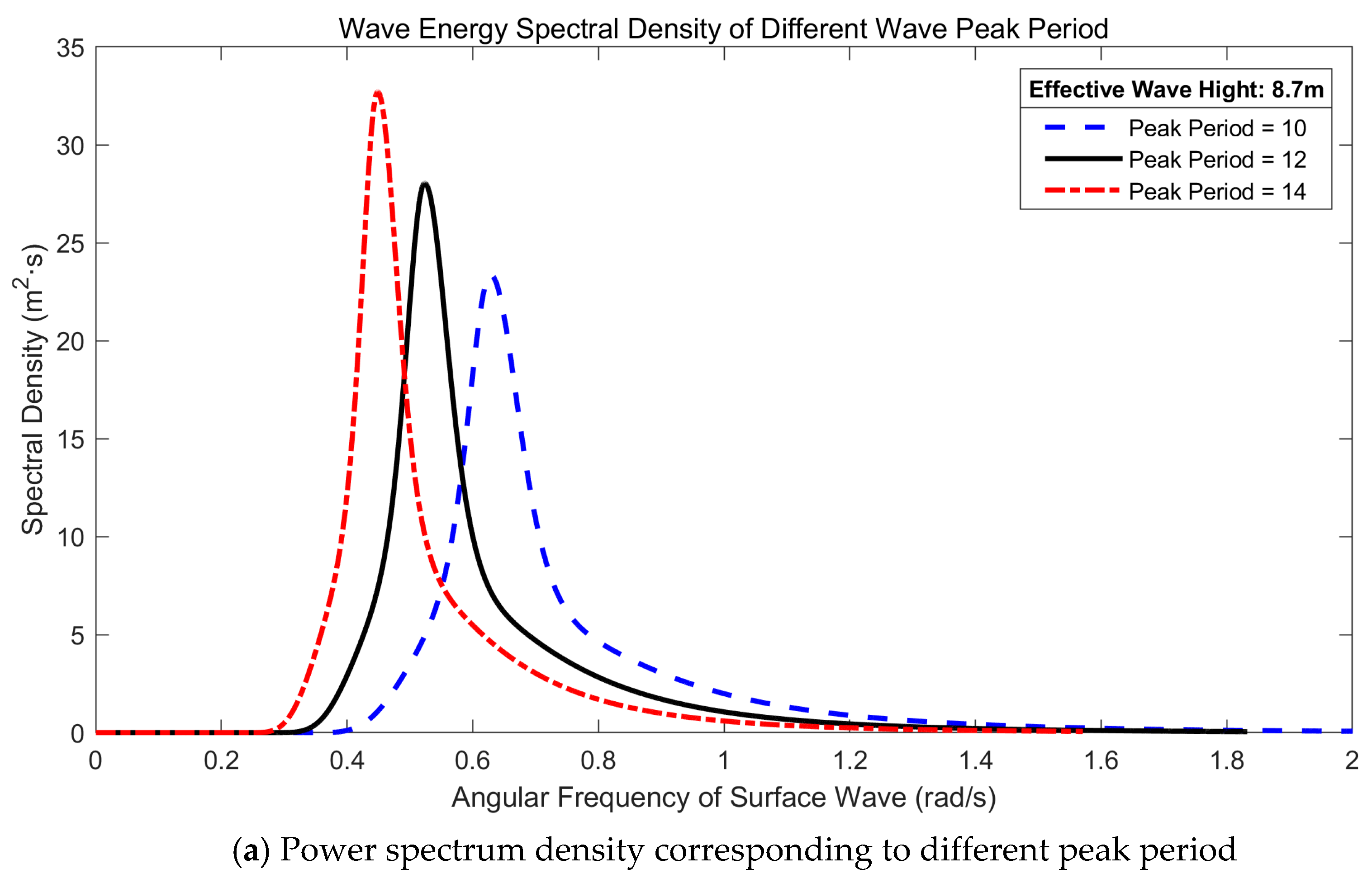
2.2.4. Combined Wave and Current Load

During the deepwater riserless casing drilling process, the drilling assembly above the seafloor is directly exposed to marine environmental load. The marine environmental load is mainly combined wave and current load. The load is related to current velocity, wave particle velocity and the velocity and acceleration of the tubular element.

The current velocity in deepwater is mainly determined by the velocity of wind induced current at sea surface and the velocity of the tidal current. The current velocity at any depth beneath the sea surface obeys the following rules [27]:

$$\{\begin{array}{ll}{U}_c=U_{\tau }{\left({\displaystyle \frac{y}{H}}\right)}^{1/7}+U_w\left({\displaystyle \frac{y+D_f-H}{D_f}}\right),\hfill & y\ge H-D_f\\ U_c=U_{\tau }{\left({\displaystyle \frac{y}{H}}\right)}^{1/7},\hfill & y<H-D_f\end{array}$$

(16)

where, U_w represents the velocity of wind induced current at the sea surface, m/s; U_t represents the velocity of tidal current at the sea surface, m/s; H represents the water depth, m; D_f represents the friction depth of wind induced current, m.

According to wind induced current theory proposed by Ekman, the velocity of wind induced current at the sea surface is as follows:

$$U_w={\displaystyle \frac{0.0127}{\sqrt{\sin \varphi }}}{V}_{wind}$$

(17)

The friction depth is as follows:

$$D_f={\displaystyle \frac{7.6}{\sqrt{\sin \varphi }}}{V}_{wind}$$

(18)

where, V_wind represents the wind velocity at the sea surface, m/s; $\varphi$ represents the latitude of the sea area, which is dimensionless.

The movement of the wave particle in deepwater can be characterized as a stationary and ergodic random process. To accurately describe the movement of wave particles under real sea conditions, the wave spectrum density function and wave theory should be properly selected.

In this study, the movements of wave particles under real sea conditions are modeled by Airy linear wave theory and JONSWAP wave spectrum density function. The Joint North Sea Wave Project (JONSWAP) spectrum is widely recognized for its ability to model the energy distribution of sea states in fetch-limited conditions, which are common in many offshore environments. Compared with the Pierson–Moskowitz spectrum, JONSWAP introduces a peak enhancement factor that better captures the sharpness of real wave peaks. This makes it especially suitable for deepwater dynamic analyses involving wave excitation, ensuring a realistic representation of environmental loading. The power spectral density of the JONSWAP spectrum is primarily determined by the effective wave height and the peak period of the wave spectrum for a given sea state. To provide a clearer understanding of how the spectral density varies with these parameters, the relationship between the power spectral density and the above two parameters are illustrated separately in Figure 5. The expression of JONSWAP wave spectrum density function is as follows [28]:

$$S_{\eta \eta }\left(\omega \right)=487\left(1-0.287\ln \gamma \right)H_s^2{T}_p^{-4}{\omega }^{-5}\times \exp \left(-1948T_p^{-4}{\omega }^{-4}\right){\gamma }^{\exp \left[-{\displaystyle \frac{{\left(0.159\omega T_P-1\right)}^2}{2{\sigma }^2}}\right]}$$

(19)

where, H_s represents the effective wave height, m; T_p represents the peak period of wave spectrum, s; $\gamma$ represents the peak enhancement factor, the observed value is 1.5~6, the mean value is 3.3; and $\sigma$ represents the peakedness factor, its value is shown as follows:

$$\sigma =\{\begin{array}{c}0.07,\begin{array}{cc}& \omega \le 2\pi /T_P\end{array}\\ 0.09,\begin{array}{cc}& \omega \le 2\pi /T_P\end{array}\end{array}$$

(20)

Since the diameter of the drilling assembly is relatively small compared with the wave length (D/L < 0.2), the forces that are exerted on the drilling assembly are mainly inertia force and drag force [29]. Thus, Morison’s equation is employed to calculate the combined wave and current force that act on the drilling assembly, and the Morison’s equation is given by the following:

$$f\left(x,t\right)=-C_A{\displaystyle \frac{\pi }{4}}{\rho }_f{D}_o^2{\dot{v}}_R^n+C_M{\displaystyle \frac{\pi }{4}}{\rho }_f{D}_o^2{\dot{v}}_w^n+{\displaystyle \frac{1}{2}}{C}_D{\rho }_f{D}_o\left(v_w^n-v_R^n\right)\left|v_w^n-v_R^n\right|$$

(21)

where, ${\rho }_f$ represent the density of sea water, kg/m³; V_wn and V_Rn represent the velocity component of a water particle that is perpendicular to the tubular element and velocity of the tubular element, respectively; V_wn and V_Rn represent the acceleration component of a water particle that is perpendicular to the tubular element and the acceleration of the tubular element, respectively; C_A represents the added mass coefficient; C_D represents the drag coefficient; and C_M represents the inertia coefficient. Of which, the relationship between added mass coefficient and inertia coefficient is as follows:

$$C_M=1+C_A$$

(22)

For the accurate calculation of the combined wave and current load, a suitable hydrodynamic coefficient should be properly selected. According to the relevant regulations of the CCS, the values of 1.20 and 1.0 are adopted for coefficients of C_D and C_A [29].

The velocity and acceleration of the centroid of tubular element can be expressed as follows:

$${\dot{v}}_R=\dot{u}\overrightarrow{i}+\dot{v}\overrightarrow{j}+\dot{w}\overrightarrow{k} {\ddot{v}}_R=\ddot{u}\overrightarrow{i}+\ddot{v}\overrightarrow{j}+\ddot{w}\overrightarrow{k}$$

(23)

Since the cross section of the drilling assembly is central symmetric, the propagation direction of wave has little to no effect on the dynamic behavior of the structure. Thus, the propagation direction of the wave is assumed to be in the position direction of the y axis. Under this condition, the velocity of a wave particle can be expressed as follows:

$${\dot{v}}_w=w_x\overrightarrow{i}+w_y\overrightarrow{j}$$

(24)

The most dangerous working condition of the drilling assembly corresponds to the one in which the propagation direction of the wave particle is coincident with that of the current particle, thus it is assumed in this study that the current also propagates along the positive direction of the y axis. In this case, the relative velocities of the water particle and the tubular element can be expressed in the following form as follows:

$${\overrightarrow{v}}_{rel}=\left(w_x-\dot{u}\right)\overrightarrow{i}+\left(w_y+U_c-\dot{v}\right)\overrightarrow{j}-\dot{w}\overrightarrow{k}$$

(25)

The expression of the velocity of the tubular element and the relative velocity of the tubular element and fluid particle that are perpendicular to the axis of drilling assembly can be derived by performing a double cross product:

$$\{\begin{array}{l}{\dot{\overrightarrow{v}}}_R^n=\left|\overrightarrow{\tau }\times {\dot{\overrightarrow{v}}}_R\times \overrightarrow{\tau }\right|\hfill \\ {\dot{\overrightarrow{v}}}_{rel}^n=\left|\overrightarrow{\tau }\times {\dot{\overrightarrow{v}}}_{rel}\times \overrightarrow{\tau }\right|\hfill \end{array}$$

(26)

where, $\overrightarrow{\tau }$ represents the tangent vector of the axis of the tubular element. According to the small rotation angle assumption, the vector can be expressed in the following form:

$$\overrightarrow{\tau }=\overrightarrow{i}+v^{\prime }\overrightarrow{j}+w^{\prime }\overrightarrow{k}$$

(27)

With the expressions stated above, the acceleration of a tubular element, the relative velocity between a water particle and tubular element and the acceleration of water particles that are perpendicular to the axis of a drilling assembly can be expressed as follows, respectively:

$$\{\begin{array}{l}{\dot{v}}_R^n=\left(\ddot{v}-\ddot{u}{v}^{\prime }\right)\overrightarrow{j}+\left(\ddot{w}-\ddot{u}{w}^{\prime }\right)\overrightarrow{k}\\ V_{rel}^n=\left[\left(w_y+U_c-\dot{v}\right)-v^{\prime }\left(w_x-\dot{u}\right)\right]\overrightarrow{j}-w^{\prime }\left(w_x-\dot{u}\right)\overrightarrow{k}\\ {\dot{v}}_w^n=\left({\dot{w}}_y-{\dot{w}}_x{v}^{\prime }\right)\overrightarrow{j}+\left(-{\dot{w}}_x{w}^{\prime }\right)\overrightarrow{k}\end{array}$$

(28)

On the basis of the above analysis, the expression for the combined wave and current loads acting on the tubular element of the drilling assembly can be expressed as follows:

$$\overrightarrow{f}\left(x,t\right)=f_y\left(x,t\right)\overrightarrow{j}+f_z\left(x,t\right)\overrightarrow{k}$$

(29)

In the above formula, $f_y\left(x,t\right)$ and $f_z\left(x,t\right)$ represents the components of the combined wave and current loads in the y axis and z axis, respectively. Their expressions are as follows:

$$\begin{array}{ll}{f}_y\left(x,t\right)& =-C_A{\rho }_f{A}_f\left(-\ddot{u}{v}^{\prime }+\ddot{v}\right)+C_M{\rho }_f{A}_f\left({\dot{w}}_y-{\dot{w}}_x{v}^{\prime }\right)\\ & +C_D{\rho }_f{r}_{outer}\left(w_y-w_x{v}^{\prime }+\dot{u}{v}^{\prime }-\dot{v}+U_c\right)\left|w_y-w_x{v}^{\prime }+\dot{u}{v}^{\prime }-\dot{v}+U_c\right|\end{array}$$

(30)

$$\begin{array}{l}{f}_z\left(x,t\right)=\\ -C_A{\rho }_f{A}_f\left(-\ddot{u}{w}^{\prime }+\ddot{w}\right)-C_M{\rho }_f{A}_f{\dot{w}}_x{w}^{\prime }+C_D{\rho }_f{r}_{outer}\left(w^{\prime }\dot{u}-w^{\prime }{w}_x\right)\left|w^{\prime }\dot{u}-w^{\prime }{w}_x\right|\end{array}$$

(31)

Thus, the virtual work achieved by the combined wave and current loads on the tubular element during the vibration process of the drilling assembly can be expressed in the following form:

$$\{\begin{array}{c}\delta W_{f_y}={\displaystyle {\int }_{x_e}^{x_e+L_e}{f}_y\left(x,t\right)\delta vdx}\\ \delta W_{f_z}={\displaystyle {\int }_{x_e}^{x_e+L_e}{f}_z\left(x,t\right)\delta wdx}\end{array}$$

(32)

2.2.5. Effect of Wet Weight of the Drilling Assembly

During the vibration process, the virtual work achieved by the buoyant weight of the tubular element can be expressed as follows:

$$\delta W_G={\displaystyle {\int }_{x_e}^{x_e+L_e}\left({\rho }_s{A}_{s}g+{\rho }_f{A}_{i}g-{\rho }_w{A}_{o}g\right)\delta udx}$$

(33)

where ${\rho }_s$, ${\rho }_f$ and ${\rho }_w$ represents the density of the tubular, drilling fluid and seawater, respectively, kg/m³; A_s is the cross-sectional area of the riser, and A_i and A_o are the inside and outside cross-sectional areas of the riser, respectively, m².

2.2.6. Effect of Contact Force Between Drill String and Wellbore Wall

During the drilling process, the contact occurs when the radial displacement of the drilling assembly center exceeds the clearance between the drilling assembly and the wellbore wall. Since the deformation of the drilling assembly in the torsional direction is not considered, there is no need to consider the friction force exerted by the wellbore wall in the tangential direction. The contact force acting on the drilling assembly can be modelled with the Hertzian contact law as follows:

$$F_{cont}=\{\begin{array}{ll}0,\hfill & \left(r-R_h-R_0\right)\le 0\\ -k_{cont}{\left(r-R_h-R_0\right)}^{3/2},\hfill & \left(r-R_h-R_0\right)>0\end{array}$$

(34)

where, $r=\sqrt{v^2+w^2}$, R_h denotes the radius of the borehole, m; R_o denotes the outer radius of the drilling assembly, m; and k_cont denotes the elastic coefficient of the contact force when the drilling assembly is in contact with the borehole wall, N/m.

With the expression of deformation potential energy, vibrational kinetic energy and the virtual work achieved by the external loads on the tubular element determined, it is necessary to perform the variational operation on the above expressions to obtain the weak form of the force equilibrium equation. Finally, appropriate shape functions are adopted to approximate the longitudinal and transverse displacements at any point along the axial direction of a tubular element, then the mass matrix M_e, stiffness matrix K_e and equivalent nodal forces vector F_e of a tubular element can be derived.

For the three dimensional coupled longitudinal-transverse vibration of a drilling assembly, each node has five degrees of freedom, which are the displacements in the direction of the three axes of the local coordinate system as well as the rotational angles of the cross section around the y- and z-axes. The degrees of freedom associated with a representative element of the structure are illustrated schematically in Figure 6.

As it can be seen from Figure 6 that this element is modeled as a two-node Euler–Bernoulli beam element, with each node possessing five degrees of freedom. Specifically, the degrees of freedom include translational displacements in the local x-, y-, and z-directions, denoted by u, v, and w, respectively, and rotational displacements about the y- and z-axes, represented by ${\theta }_y$ and ${\theta }_z$.

At Node 1 (left end), the degrees of freedom are denoted as u₁, v₁, w₁, ${\theta }_{y1}$, and ${\theta }_{z1}$; similarly, at Node 2 (right end), they are labeled u₂, v₂, w₂, ${\theta }_{y2}$ and ${\theta }_{z2}$. These degrees of freedom fully describe the kinematic behavior of each element within the finite element model of the drillstring.

Since the effect of shear force on the rotation of the cross section is not considered, the nodal displacement vector of a tubular element can be expressed as follows:

$$q_e^T=\{u_1\begin{array}{cc}& v_1\begin{array}{cc}& {v_1}^{\prime }\begin{array}{cc}\begin{array}{cc}& w_1\begin{array}{cc}& {w_1}^{\prime }\end{array}\end{array}& u_2\begin{array}{cc}& v_2\begin{array}{cc}& {v_2}^{\prime }\begin{array}{cc}& w_2\begin{array}{cc}& {w_2}^{\prime }\}\end{array}\end{array}\end{array}\end{array}\end{array}\end{array}\end{array}$$

(35)

In this study, a linear shape function and a Hermite cubic interpolation function are respectively adopted to approximate the longitudinal and transverse displacement of any point along the axial direction of a tubular element. The longitudinal displacement as well as the transverse displacement of any point along the axial direction of a tubular element can be expressed in the following form:

$$u=N_u{q}_e,\begin{array}{cc}& v=N_v\end{array}{q}_e,\begin{array}{cc}& w=N_w{q}_e\end{array}$$

(36)

where, N_u represents the shape function vector of displacement in the x-axis direction, N_v and N_w represent the shape functions vector of displacement in the y-axis and z-axis respectively, and the dimensionless length $\xi =x/l$ is defined for a tubular element of length l. Then the shape function vectors can be expressed in the following form:

$$\begin{array}{l}{N}_u=\{N_{u1}\begin{array}{cc}& 0\begin{array}{cc}& 0\begin{array}{cc}\begin{array}{cc}& 0\begin{array}{cc}& 0\end{array}\end{array}& N_{u2}\begin{array}{cc}& 0\begin{array}{cc}& 0\begin{array}{cc}& 0\begin{array}{cc}& 0\}\end{array}\end{array}\end{array}\end{array}\end{array}\end{array}\end{array}\\ N_v=\{0\begin{array}{cc}& N_{v1}\end{array}\begin{array}{cc}& N_{v2}\begin{array}{cc}\begin{array}{cc}& 0\begin{array}{cc}& 0\begin{array}{cc}& 0\end{array}\end{array}\end{array}& \begin{array}{cc}& N_{v3}\begin{array}{cc}& N_{v4}\begin{array}{cc}& 0\begin{array}{cc}& 0\}\end{array}\end{array}\end{array}\end{array}\end{array}\end{array}\\ N_w=\{0\begin{array}{cc}& 0\end{array}\begin{array}{cc}& 0\begin{array}{cc}\begin{array}{cc}& N_{w1}\begin{array}{cc}& N_{w2}\begin{array}{cc}& 0\end{array}\end{array}\end{array}& \begin{array}{cc}& 0\begin{array}{cc}& 0\begin{array}{cc}& N_{w3}\begin{array}{cc}& N_{w4}\}\end{array}\end{array}\end{array}\end{array}\end{array}\end{array}\end{array}$$

(37)

of which,

$$\begin{array}{ll}{N}_{u1}=1-\xi , N_{u2}=\xi ,& \\ N_{v1}=1-3{\xi }^2+2{\xi }^3,& N_{v2}=\xi l{\left(1-\xi \right)}^2,\\ N_{v3}={\xi }^2\left(3-2\xi \right),& N_{v4}={\xi }^{2}l\left(\xi -1\right)\\ N_{w1}=1-3{\xi }^2+2{\xi }^3,& N_{w2}=-\xi l{\left(1-\xi \right)}^2,\\ N_{w3}={\xi }^2\left(3-2\xi \right),& N_{w4}=-{\xi }^{2}l\left(\xi -1\right)\end{array}$$

(38)

By bringing the approximate form of the above displacement equations into the variational expressions of the strain potential energy, kinetic energy and the virtual work achieved by the external load of the tubular element, the specific expressions of the mass matrix, stiffness matrix, damping matrix and equivalent nodal force vector of the tubular element can be derived. Then, after assembling the mass matrix, stiffness matrix and equivalent nodal force vector of the tubular elements according to the connection relationship in the overall structure, the nonlinear dynamic finite element governing equation of the drilling assembly can be derived as follows:

$$\begin{array}{r}\left(\left[M\right]+\left[M_f\right]\right)\left\{\ddot{q}\right\}+\left(\left[C\right]+\left[C_f\right]\right)\left\{\dot{q}\right\}+\left(\left[K_L\right]+\left[K_{NL}\left(q\right)\right]+\left[K_f\right]\right)\left\{q\right\}\\ =\left\{F_{NL}\left(t,q,\dot{q},\ddot{q}\right)\right\}\end{array}$$

(39)

where, $\left\{\ddot{q}\right\}$ and $\left\{\dot{q}\right\}$ denotes respectively the nodal acceleration and velocity vector of the overall structure; M, C, K_L and K_NL denotes respectively the mass matrix, damping matrix, linear and nonlinear parts of the stiffness matrix of the overall drilling assembly without considering the effect of flowing drilling fluid; M_f, C_f and K_f denotes respectively the mass matrix, damping matrix and stiffness matrix resulting from the effect of the flowing drilling fluid; $\left\{F_{NL}\left(t,q,\dot{q},\ddot{q}\right)\right\}$ denotes the force vectors acting on the overall structure, which include the combined wave and current load acting perpendicular to the axis of the drilling assembly, the buoyant weight of the assembly itself, the force of the flowing drilling fluid acting tangentially to the axis of the drilling assembly, and the contact force between drilling assembly and wellbore wall.

Equation (39) is the finite element governing equation for the three-dimensional coupled longitudinal-transverse vibration of the drilling assembly during the deepwater surface casing drilling process. Since the stiffness matrix and the force vector contain the displacement, velocity and acceleration of the drilling assembly, an iterative solution method is required.

2.3. Boundary Conditions

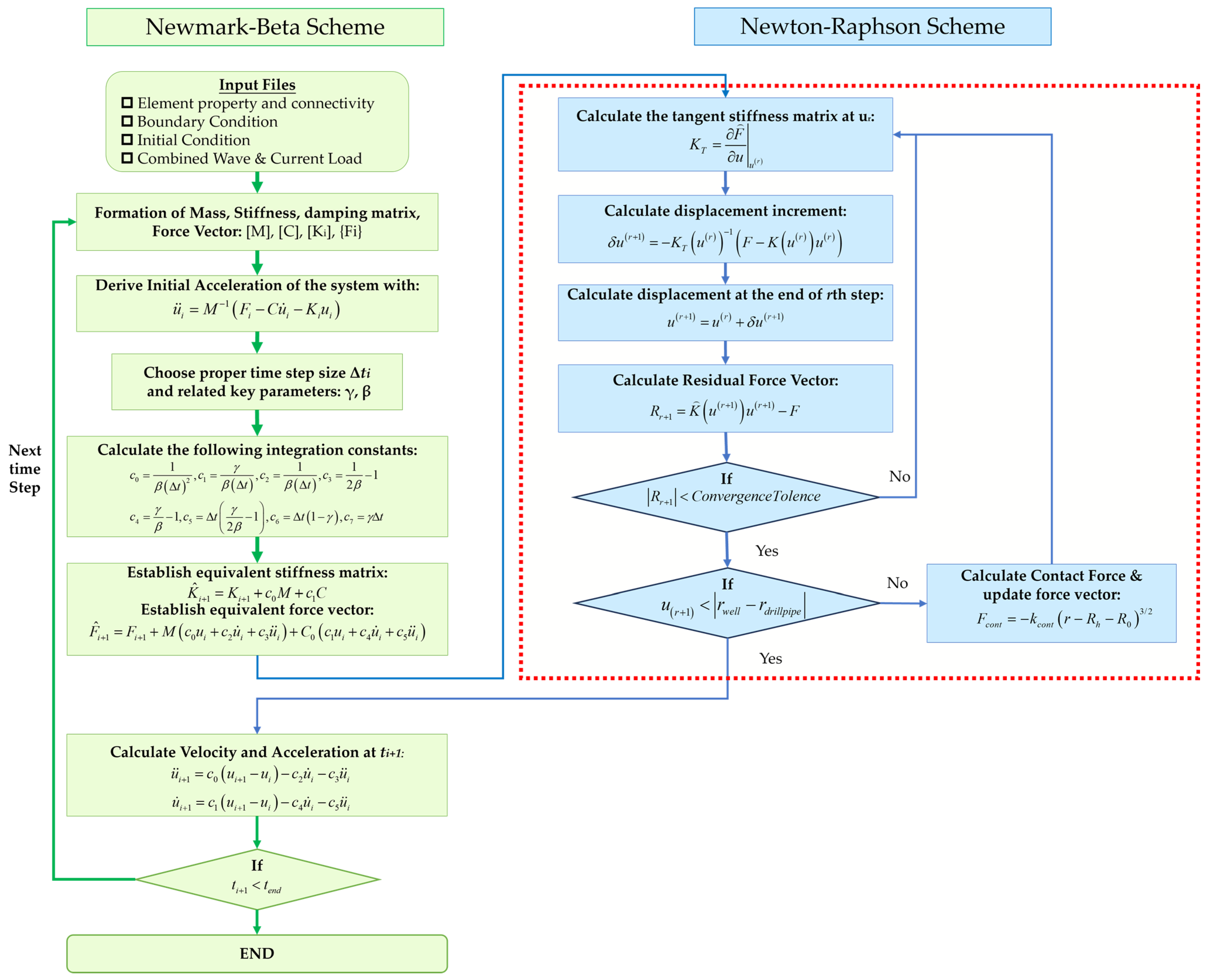
In order to derive the vibration state of the drilling assembly, the boundary conditions should also be explicitly specified.

In the deepwater surface casing drilling process, the upper end of the drilling assembly is connected to the hook, and the drag force exerted by the hook on the top end of the drilling assembly depends on the weight on the bit. Since the drilling assembly is driven by the rotary table, the top end of the drilling assembly can be considered to be rigidly supported in the transverse direction. Thus, the boundary condition at the top end of the drilling assembly can be expressed as follows:

$$\begin{array}{r}{E{A}_{oL}\left(u^{\prime }+{\displaystyle \frac{1}{2}}{v^{\prime }}^2+{\displaystyle \frac{1}{2}}{w^{\prime }}^2\right)|}_{0,t}=-T_{hl}\\ v\left(0,t\right)=0\\ E{I}_{oL}{v}^{″}\left(0,t\right)=0\\ w\left(0,t\right)=0\\ E{I}_{oL}{w}^{″}\left(0,t\right)=0\end{array}$$

(40)

Since the shallow layer of the seabed is unconsolidated, the drill bit can be assumed to be always in the center of the wellbore and remains in continuous contact with the formation. Thus, the bottom end boundary condition of the drilling assembly can be expressed as follows:

$$\begin{array}{r}{E{A}_{oC}\left(u^{\prime }+{\displaystyle \frac{1}{2}}{v^{\prime }}^2+{\displaystyle \frac{1}{2}}{w^{\prime }}^2\right)|}_{0,t}=-N_{wob}\left(t\right)\\ v\left(L_c,t\right)=0\\ E{I}_{oC}{v}^{″}\left(L_c,t\right)=0\\ w\left(L_c,t\right)=0\\ E{I}_{oC}{w}^{″}\left(L_c,t\right)=0\end{array}$$

(41)

where A_oL and A_oC denote the cross-sectional area of the landing string and casing, respectively, m²; I_oL and I_oC denote the moment of inertia of the cross section of the landing string and casing, respectively, m⁴, and L_c denotes the bottom end position of the casing in global Cartesian coordinate system, m; T_hl denotes the hook load, N, and N_wob denotes the fluctuating weight on bit, N.

3. Solution Method

To solve the established nonlinear dynamic equations, the Newmark-β method combined with the Newton–Raphson method will be used in this analysis.

The Newmark-β integration scheme is primarily selected for its unconditional stability and robustness when solving nonlinear structural dynamics problems. Coupled with the Newton–Raphson iterative method, it efficiently handles nonlinearities arising from contact interactions and large displacements, making it especially suitable for the nonlinear dynamic analysis presented in this study. In analyzing and solving the dynamic problem with the Newmark-β method, the excitation function and the response history of the system are firstly divided into certain time intervals in the time domain, and then the dynamic response of the system at the end of each time step is solved by the differential equation of motion according to the initial state (displacement and velocity) and the excitation’s time history function during each time step. To this end, the displacement, velocity and acceleration of the system at the time t = 0 can be incrementally extrapolated to the response of the system at any time according to the pre-divided time interval.

When applying the incremental time stepping scheme, the temporal evolution of the acceleration within this time step should be determined firstly. N. M. Newmark proposed the Newmark-β method by introducing the parameters γ and β on the basis of the average acceleration method and the linear acceleration method [18]. In this method, the final velocity as well as displacement can be derived by the following expression for each time step [30]:

$${\dot{u}}_{i+1}={\dot{u}}_i+\left[\left(1-\gamma \right)\Delta t\right]{\ddot{u}}_i+\left(\gamma \Delta t\right){\ddot{u}}_{i+1}$$

(42)

$$u_{i+1}=u_i+\left(\Delta t\right){\dot{u}}_i+\left[\left(0.5-\beta \right){\left(\Delta t\right)}^2\right]{\ddot{u}}_i+\left[\beta {\left(\Delta t\right)}^2\right]{\ddot{u}}_{i+1}$$

(43)

The dynamic equilibrium equation of the system at $t_{i+1}$ is shown below:

$$M{\ddot{u}}_{i+1}+C{\dot{u}}_{i+1}+K{u}_{i+1}=F_{i+1}$$

(44)

In order to derive the response at time t_i+1 from that at time t_i, it is necessary to express the velocity and the acceleration of the system at time t_i+1 in terms of the displacement, velocity, and acceleration at time t_i as well as the displacement of the system at time t_i+1 according to Equations (45) and (46), that is:

$${\ddot{u}}_{i+1}={\displaystyle \frac{1}{\beta {\left(\Delta t\right)}^2}}\left(u_{i+1}-u_i\right)-{\displaystyle \frac{1}{\beta \left(\Delta t\right)}}{\dot{u}}_i-\left({\displaystyle \frac{1}{2\beta }}-1\right){\ddot{u}}_i$$

(45)

$${\dot{u}}_{i+1}={\displaystyle \frac{\gamma }{\beta \left(\Delta t\right)}}\left(u_{i+1}-u_i\right)+\left(1-{\displaystyle \frac{\gamma }{\beta }}\right){\dot{u}}_i+\Delta t\left(1-{\displaystyle \frac{\gamma }{2\beta }}\right){\ddot{u}}_i$$

(46)

Finally, by bringing the above expression into the dynamic equilibrium equation, the equation that can be used to solve the displacement of the system at time t_i+1 can be derived:

$$\widehat{K}{u}_{i+1}={\widehat{F}}_{i+1}$$

(47)

Of which, the expressions of ${\widehat{K}}_{i+1}$ and ${\widehat{F}}_{i+1}$ are shown below:

$$\widehat{K}=K+{\displaystyle \frac{1}{\beta {\left(\Delta t\right)}^2}}M+{\displaystyle \frac{\gamma }{\beta \left(\Delta t\right)}}C$$

(48)

$$\begin{array}{ll}{\widehat{F}}_{i+1}& =F_{i+1}+M\left[{\displaystyle \frac{1}{\beta {\left(\Delta t\right)}^2}}{u}_i+{\displaystyle \frac{1}{\beta \left(\Delta t\right)}}{\dot{u}}_i+\left({\displaystyle \frac{1}{2\beta }}-1\right){\ddot{u}}_i\right]\\ & +C\left[{\displaystyle \frac{\gamma }{\beta \left(\Delta t\right)}}{u}_i+\left({\displaystyle \frac{\gamma }{\beta }}-1\right){\dot{u}}_i+\Delta t\left({\displaystyle \frac{\gamma }{2\beta }}-1\right){\ddot{u}}_i\right]\end{array}$$

(49)

For the computational stability of Newmark-β method, the time step size should satisfy the following conditions:

$${\displaystyle \frac{\Delta t}{T}}\le {\displaystyle \frac{1}{\sqrt{2}\pi }}{\displaystyle \frac{1}{\sqrt{\gamma -2\beta }}}$$

(50)

where $\Delta t$ denotes the computational time step size, s; and T denotes the minimum natural vibration period of the system, s. Typically, the value of parameters γ and β are set as follows:

$$\gamma =1/2, 1/6\le \beta \le 1/4$$

(51)

For nonlinear dynamic problems, the system stiffness matrix K and the nodal load vectors F over time also needs to be considered when analyzing and solving the problem using the computational procedure described above. Thus, the nodal displacement vectors of the system at the end of each time step are solved using the equivalent stiffness matrix and the equivalent nodal load vectors by means of the Newton-Raphson method.

The Newton–Raphson method is adopted to address the geometric nonlinearity of the drilling assembly deformation and the contact nonlinearity between drill pipe and the wellbore wall. By coupling it with the Newmark-β integration scheme, the transient nonlinear problem is converted into a series of quasi-static nonlinear problems. In each time step, the tangent stiffness matrix is linearized based on the current displacement estimate, and the force vector is updated to account for contact effects. The residual force vector is calculated, and convergence is evaluated against a predefined tolerance criterion. If convergence is not achieved, the displacement increment is recalculated and the process repeats until convergence is satisfied. Once the displacement is obtained, the velocity and acceleration are subsequently updated using the Newmark-β formulas, as shown in Equations (45) and (46). The overall iterative process is summarized in the flowchart presented in Figure 7, where $K_T$ denotes the tangent stiffness matrix and $R_{i+1}$ represents the residual force vector at iteration i + 1.

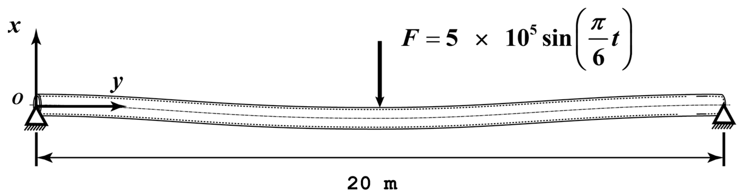
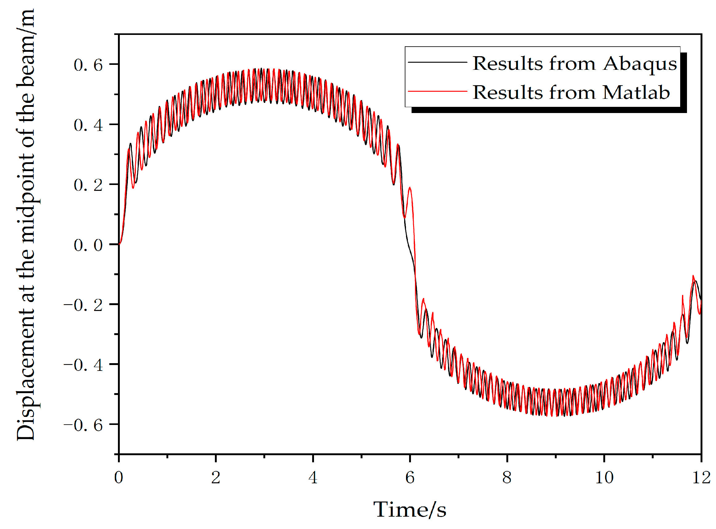
4. Model Verifications

In this study, a finite element program was developed in MATLAB 2014a to analyze the dynamic response of the integrated drillstring system based on the aforementioned solution method. To verify the accuracy of the program, a comparison was conducted between the simulation results obtained from the developed program and those from the commercial software Abaqus 6.14. The test model consisted of a slender beam with pinned supports at both ends and subjected to a periodic concentrated load at its mid-span. A schematic of the beam structure is shown in Figure 8. The inner and outer diameters of the beam are 0.05 m and 0.07 m, respectively, with a total length of 20 m. The applied periodic load has an amplitude of 500 kN and a period of 12 s.

This study primarily compares the time-history of displacement in the y-direction at the midpoint of the beam obtained from two different solution approaches. The comparison results are illustrated in Figure 9. As shown in Figure 9, the results computed by the proposed program closely match those obtained from Abaqus, indicating that the developed finite element program possesses a high level of accuracy and reliability.

5. Engineering Applications

In this study, the data of a deep water well in the South China Sea are taken as an example, the actual operating water depth of the well is 1272 m, the surface casing is expected to be set to 1320 m below the mudline. In this analysis, it is assumed that the well has been drilled up to 400 m below the mudline, thus, the total length of the casing string that is exposed to seawater will be 920 m, and the total length of the landing string will be 352 m. The specific parameters related to the landing string and the casing are listed in

Table 1. Characteristics of the tubulars pertaining to the landing string assembly.

Physical Property	Landing String	Casing
Outer diameter (mm)	168.3	508
Inner diameter (mm)	135.8	476.25
Wall thickness (mm)	16.25	15.875
Cross-sectional area (mm2)	7762	24,544
Line weight (N·m−1)	718.13	1888.2
Length (m)	352	1320
Material property	S-135	X56
Tensile strength (kN)	7221.4	9600
Bending stiffness (N·m2)	4,764,574.4	1,532,211.8
Yield strength (Mpa)	930.7	390

.

The density of seawater in the drilling operation area is 1025 kg/m³, the wind speed at the sea surface is 6.4 m/s, the current velocity at the sea surface is 0.15 m/s, the drag force coefficient is taken as 1.2, the inertia force coefficient is taken as 2.0, the effective wave height is 8.7 m, the peak period of the wave is 12.3 s, and the peak enhancement factor γ of the JONSWAP spectrum is 3.3.

Assuming that the flow rate of drilling fluid during the drilling operation of the deepwater surface section is 1500 gal/min (that is, 0.0946 m³/s) and the drilling pressure exerted on the drill bit is 100 kN, the fluctuation of drilling pressure at the bottom due to the interaction between the drill bit and the rock is a sinusoidal fluctuation function, and the expression of fluctuation function is: $50\sin 2\pi t$ (kN).

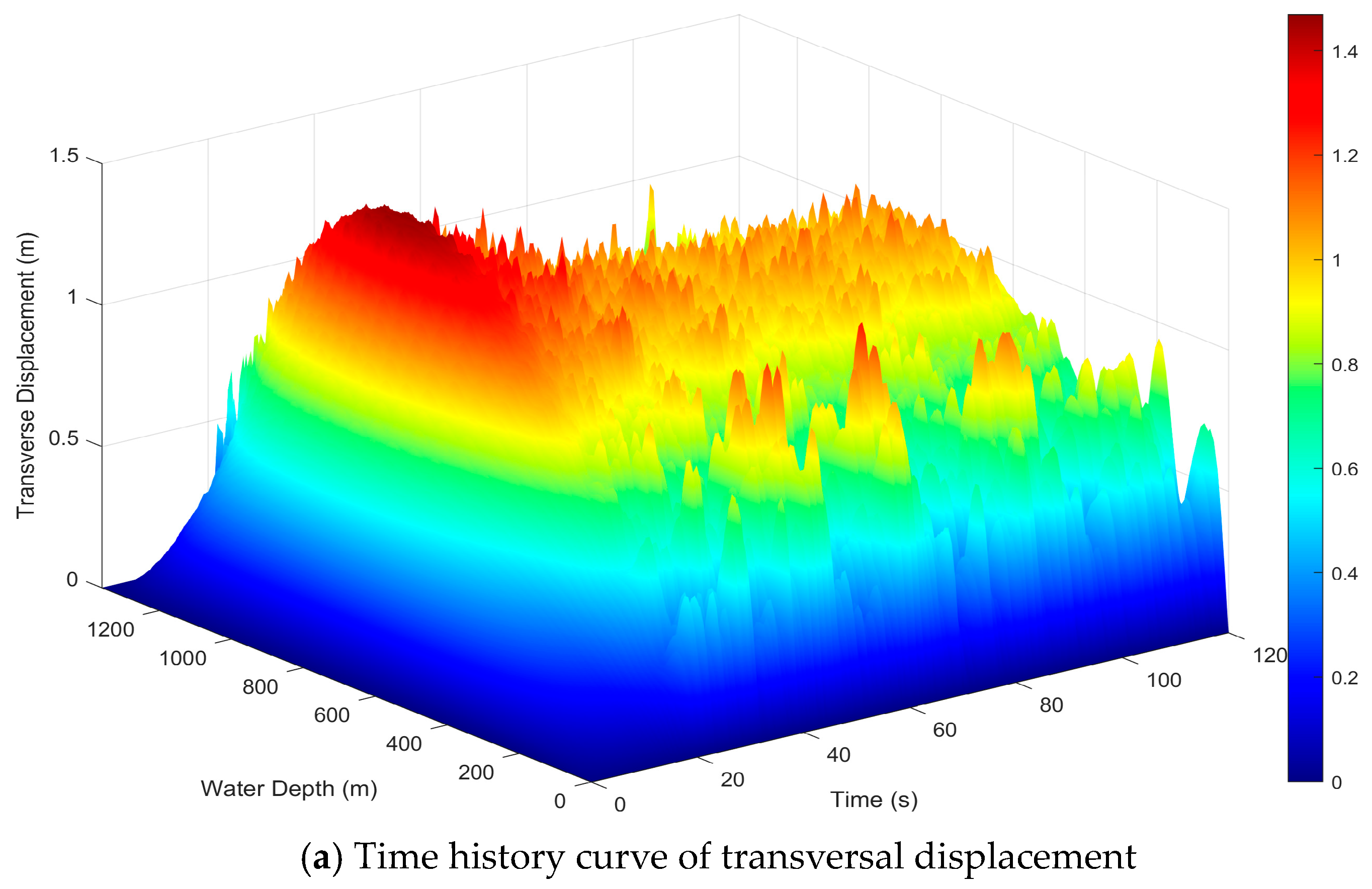
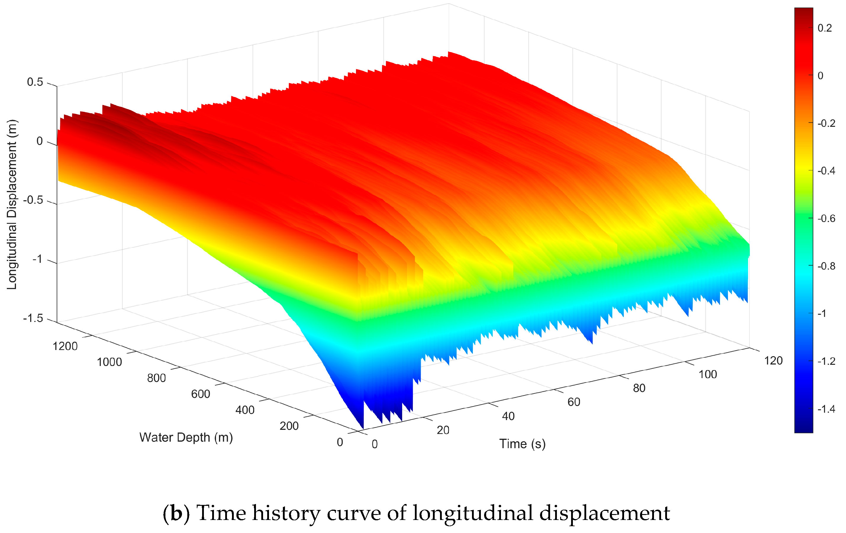
5.1. Dynamic Displacement Profile of the Drillstring

Figure 10 presents the time-history curves of the longitudinal and transverse displacements of any point on the drillstring and in the seawater section during the deepwater surface casing drilling process. It is evident that the longitudinal and transverse displacements of these points are maximal during the initial phase of vibration, subsequently diminishing and reaching a stable vibratory state. In the initial vibration phase, the peak transverse displacement occurs in the midsection of the casing, while the maximum longitudinal displacement is observed at the top end of the landing string, both the longitudinal displacement and its fluctuation amplitude on the landing string are significantly greater than the corresponding values on the casing. During the stable vibration state, the casing exhibit relatively small longitudinal displacements and fluctuation amplitudes, whereas the transverse displacement remains relatively large with noticeable minor oscillations. Conversely, for the landing string, both the longitudinal displacement and its fluctuation amplitude are remarkably greater than those on the casing, and the transverse displacement exhibits considerable oscillatory behavior.

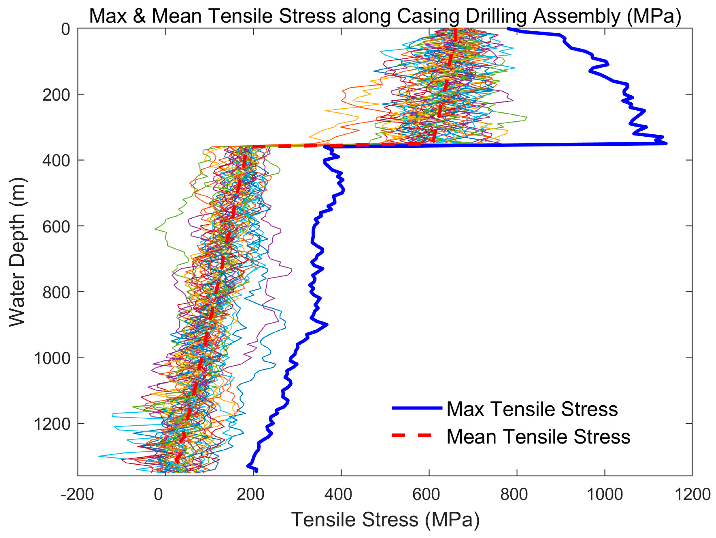
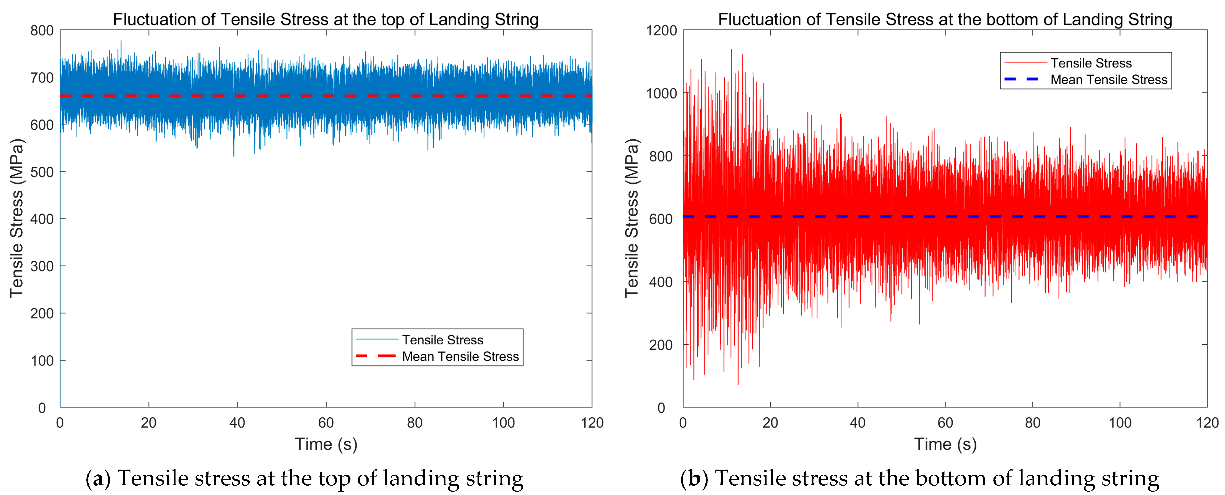
5.2. Distribution of Tensile Stresses on the Drillstring

Figure 11 depicts the axial tensile stress distribution along the casing drilling assembly in the seawater section. The data indicates that the mean axial tensile stress in the landing string decreases progressively with the increase of water depth, while the extreme values exhibit an increasing trend. In contrast, both the mean and extreme axial tensile stresses in the casing diminish with the increase of water depth. These observations align with the patterns observed in the time-history curves of longitudinal and transverse displacements of the whole drillstring.

Figure 12 illustrates the time-history curves of tensile stress at both the top and bottom end of the landing string during its drilling process. As depicted in Figure 12a, the tensile stress at the top of the landing string remains in a stable fluctuating state throughout the drilling process, with an average value of 536 MPa and a fluctuation amplitude of approximately 35 MPa. In contrast, Figure 12b shows that the fluctuation amplitude of tensile stress at the bottom of the landing string is significantly larger during the drilling process. Initially, the fluctuation amplitude at the bottom reaches its maximum, averaging around 310 MPa. Upon reaching a stable vibration state, this amplitude suddenly decreases to an average of about 180 MPa and stabilizes within a certain range. Although the mean tensile stress at the top of the landing string is higher, the extreme values of tensile stress at the bottom substantially exceed those at the top.

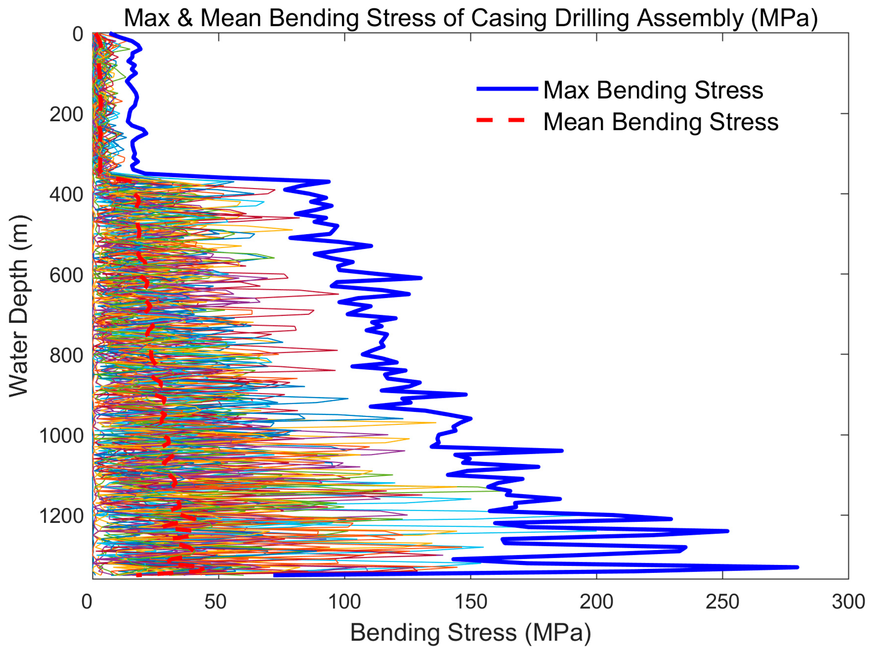
5.3. Distribution of Bending Stresses on the Casing Drilling Assembly

Figure 13 illustrates the bending stress distribution along the drillstring in the seawater section during its nonlinear vibration process. The data reveals that both the mean and extreme values of bending stress on the casing are significantly greater than the corresponding values on the landing string. Throughout the nonlinear vibration process, the mean and extreme bending stresses on the landing string remain relatively low and exhibit minor variation along the axial direction. In contrast, the casing experiences higher mean and extreme bending stresses, which show an approximately linear increase with the increase of water depth. Additionally, the fluctuation amplitude of bending stress along the axial direction of the casing becomes more pronounced closer to the lower end of the pipe string.

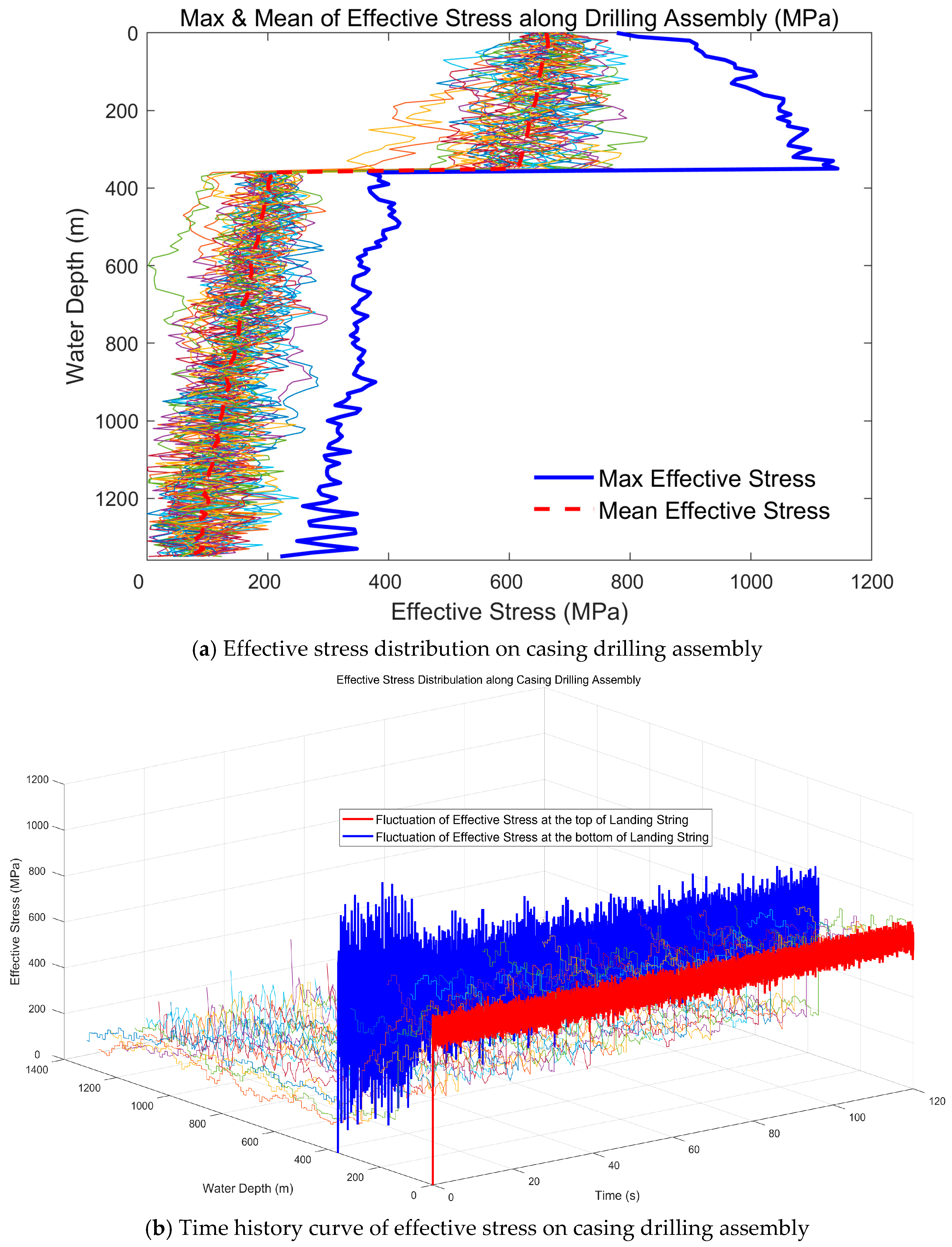
5.4. Distribution of Effective Stress on the Casing Drilling Assembly

Figure 14 illustrates the distribution and temporal variation of effective stress along the axial direction of the drillstring in the seawater section during its nonlinear vibration process. A comparison between Figure 11 and Figure 14a reveals that, throughout the vibration process, the distribution pattern of effective stress mirrors that of axial tensile stress. Specifically, both the mean and extreme values of effective stress on the landing string are significantly higher than those on the casing string. For the entire seawater section of the drillstring, the maximum value of the mean effective stress occurs at the top of the landing string, while the maximum value of extreme effective stress is observed at its bottom end. The phenomenon is primarily attributed to the fact that, the fluctuation amplitude of the effective stress on the landing string increases with the increase of water depth during the nonlinear vibration process. As it can be seen from Figure 14b, the fluctuation amplitude of effective stress at the bottom of the landing string consistently surpasses that at the top throughout the vibration process. The top of the landing string exhibits a smaller, stable fluctuation amplitude, whereas the bottom experiences larger fluctuations, and reaches its peak value during the initial vibration phase. Upon reaching a stable vibration state, these fluctuations at the bottom suddenly decrease and stabilize within a specific range. In the stable vibration state, the mean effective stress at the top of the landing string is 541 MPa with a fluctuation amplitude of approximately 24 MPa, while at the bottom, the mean effective stress is 508 MPa with a fluctuation amplitude of about 153 MPa.

5.5. Parameter Sensitivity Analysis

Based on the analysis above, it is evident that during the deepwater surface casing drilling process, the landing string experiences significant extreme values in tensile stress, bending stress, and effective stress, potentially leading to yield failure of the pipe string. Therefore, it is essential to investigate the factors influencing the stress distribution within the drillstring to implement appropriate measures for controlling the stress distribution across the pipe string’s cross-section. Typically, factors affecting the stress distribution of the drillstring include drilling engineering parameters—such as weight on bit (WOB), drill string rotational speed, and drilling fluid flow rate, and physical properties of the pipe string, including wall thickness and material density. Modifying drilling engineering parameters can impact drilling efficiency; thus, altering these parameters is generally not recommended. This study focuses on analyzing changes in stress distribution resulting from variations in the physical properties of the pipe string.

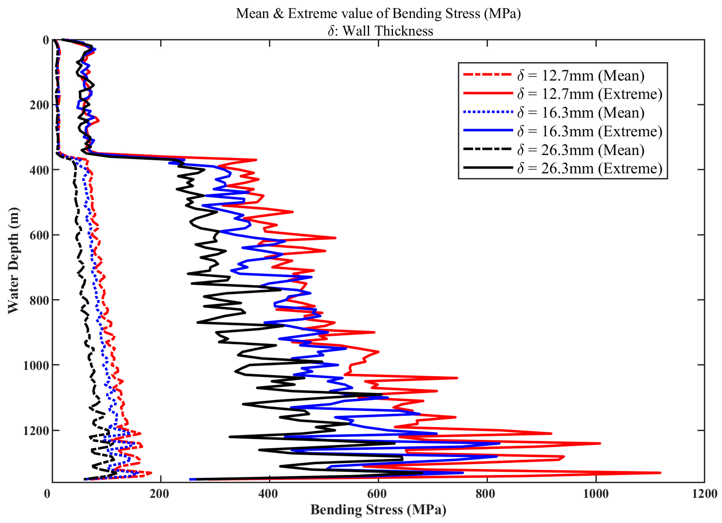
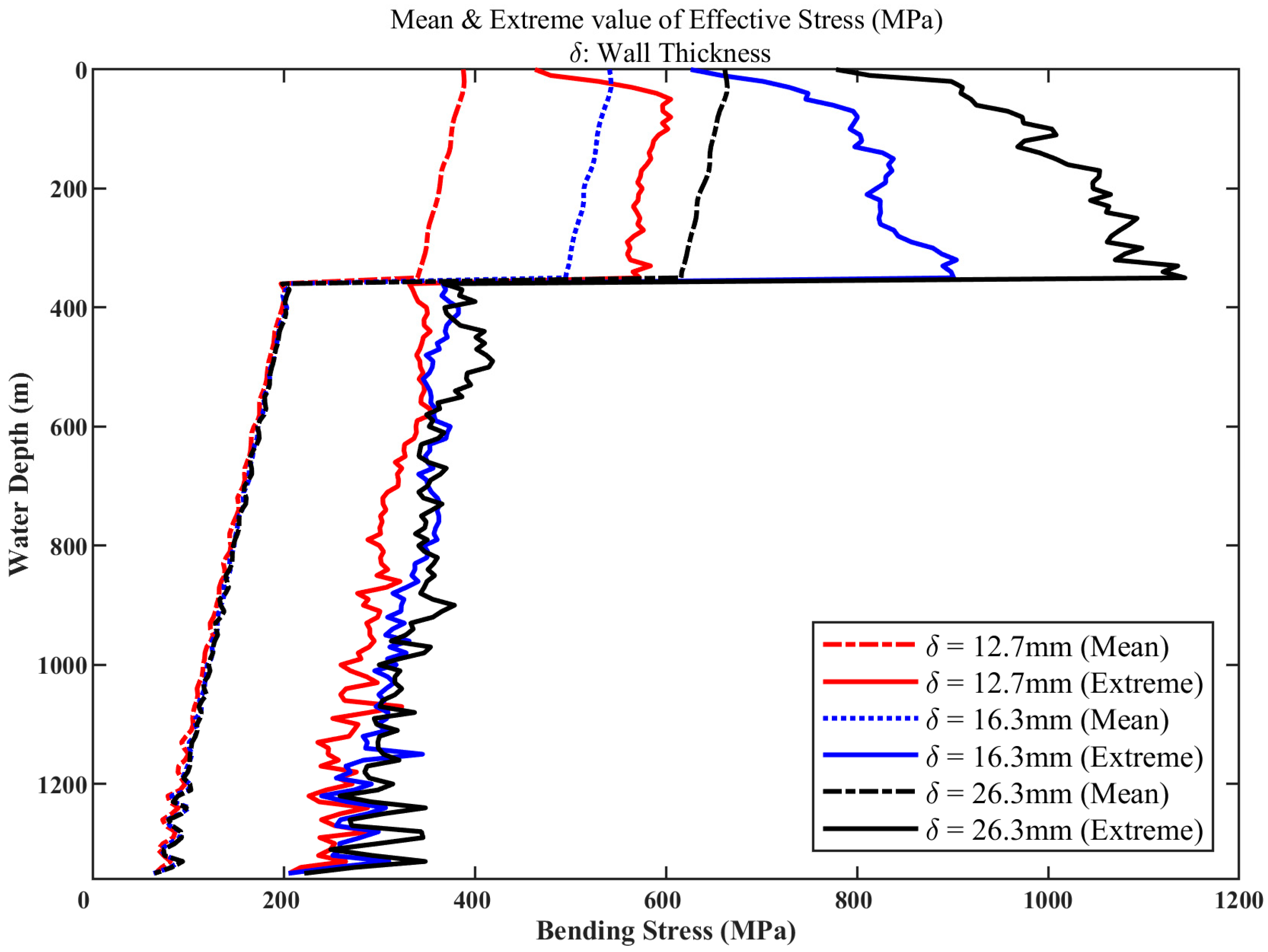
5.5.1. Effect of Wall Thickness

In addition to the landing string specifications mentioned in the previous example, another commonly used specification in the field features an outer diameter of 168.3 mm, an inner diameter of 149.2 mm, and a wall thickness of 12.7 mm. For comparative analysis, this study also considers a hypothetical landing string with an outer diameter of 168.3 mm, an inner diameter of 115.8 mm, and a wall thickness of 26.25 mm. The primary focus is to analyze the variations in the mean and extreme values of axial tensile stress, bending stress, and effective stress along the axial direction of the operating pipe string under different wall thicknesses.

(1)

Comparison of axial tensile stress

Figure 15 illustrates the distribution of mean and extreme axial tensile stresses along the landing string and casing for different wall thicknesses. In the figure, dashed lines represent mean axial tensile stresses, while solid lines denote extreme values. A comparative analysis reveals that increasing the wall thickness significantly reduces both the mean and extreme axial tensile stresses along the landing string. Moreover, a thicker wall results in a smaller difference between the mean and extreme stresses, indicating reduced stress fluctuation during vibration. Therefore, selecting a landing string with a larger wall thickness can effectively decrease axial tensile stress.

(2)

Comparison of bending stress

Figure 16 illustrates the distribution of mean and extreme bending stresses along the axial direction of the landing string and casing for varying wall thicknesses. The data indicates that increasing the wall thickness of the landing string leads to a noticeable reduction in both the mean and extreme bending stresses on the casing. Since the bending stress on the landing string is relatively low, changes in its wall thickness do not significantly affect its bending stress.

(3)

Comparison of effect stress

Figure 17 illustrates the variations in mean and extreme effective stresses along the axial direction of both the landing string and casing under different wall thicknesses. The data indicates that changes in effective stress closely mirror those observed in axial tensile stress. Specifically, as the wall thickness of the landing string increases, there is a significant reduction in effective stress. In contrast, the mean effective stress in the casing remains largely unaffected by changes in the landing string’s wall thickness, while the extreme values exhibit a slight decrease.

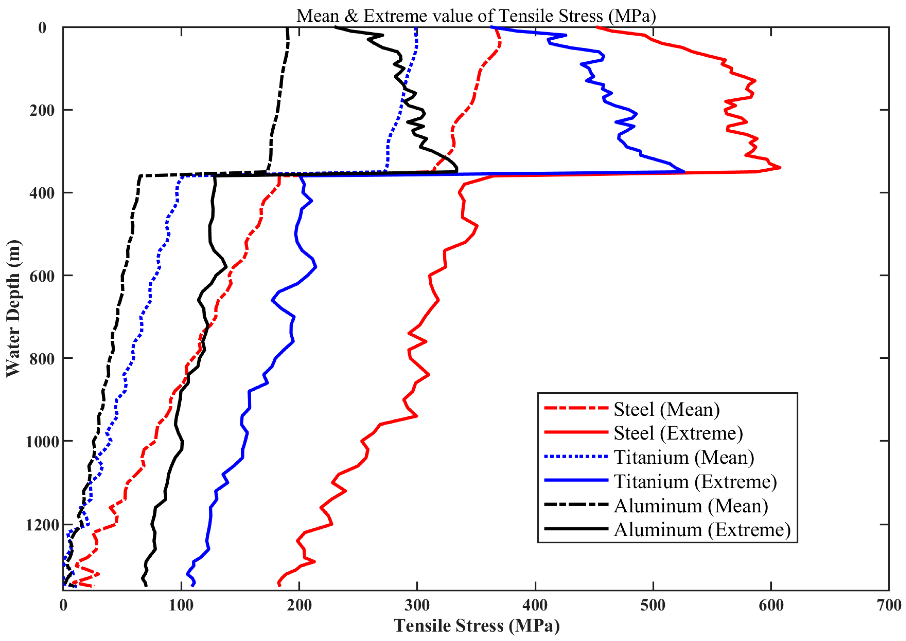
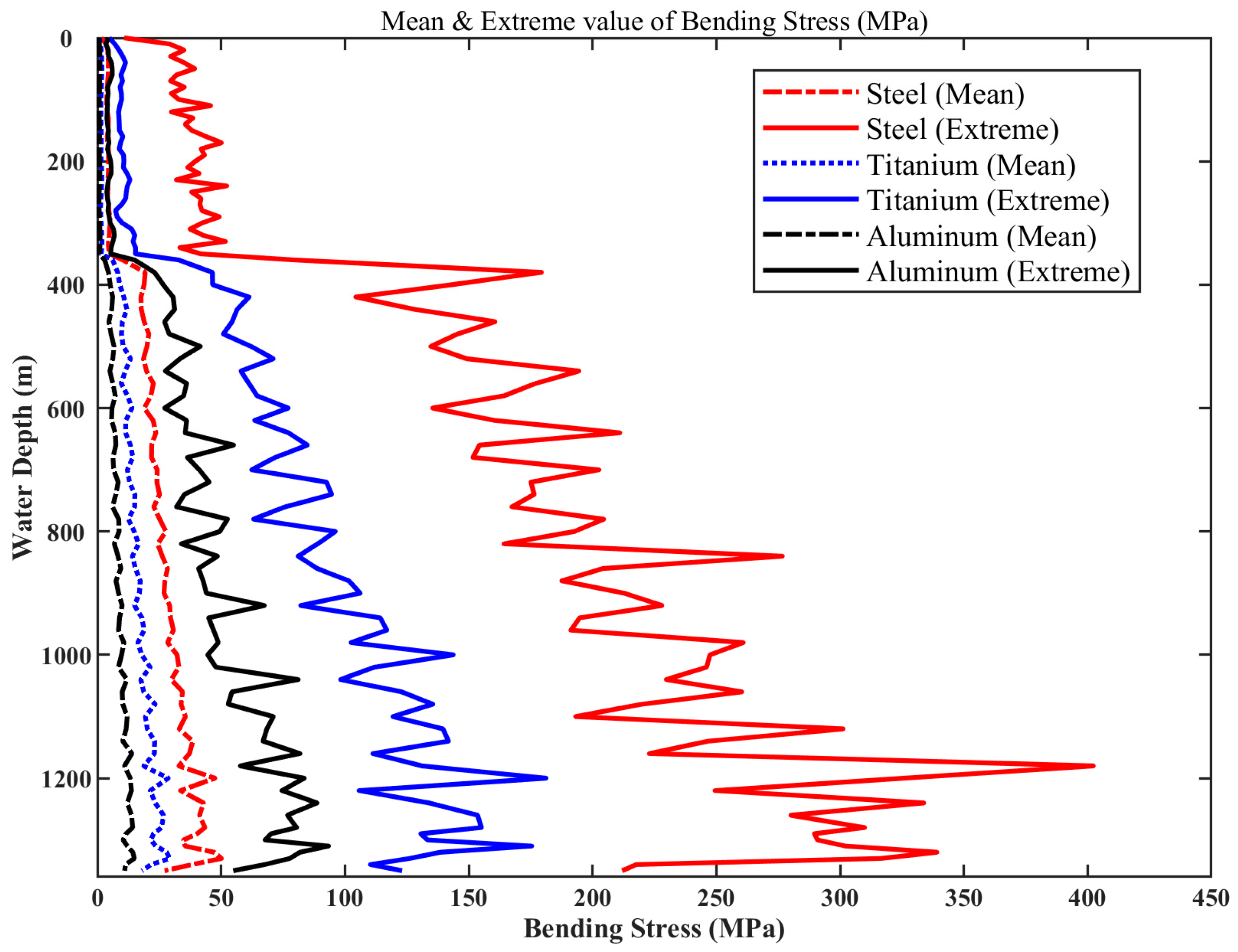
5.5.2. Effect of Pipe String Material

With advancements in drilling technology, contractors developed new types of drill string materials to address complex operational conditions. Commonly used new materials include aluminum alloy and titanium alloy drill strings. These materials typically have lower densities, effectively reducing the stress on the drill string during operations, thereby enhancing safety. Standard titanium alloy drill strings have a density of 4410 kg/m³, a Young’s modulus of 114 GPa, and a yield strength of 827 MPa. Standard aluminum alloy drill strings have a density of 2800 kg/m³, a Young’s modulus of 72 GPa, and a yield strength of 330 MPa.

(1)

Comparison of tensile stress

Figure 18 illustrates the variations in mean and extreme axial tensile stresses along the landing string and casing for different pipe string materials. The data indicates that as the material density decreases, the axial tensile stresses in both the landing string and casing significantly diminish. Furthermore, materials with lower densities exhibit reduced stress fluctuation amplitudes. Therefore, selecting pipe string materials with lower densities can effectively reduce axial tensile stresses.

(2)

Comparison of bending stress

Figure 19 illustrates the variations in mean and extreme bending stresses along the axial direction of the landing string and casing for different pipe string materials. The data indicates that as the material density decreases, the bending stresses in both the landing string and casing significantly diminish. Moreover, materials with lower densities exhibit reduced stress fluctuation amplitudes. Therefore, selecting pipe string materials with lower densities can effectively reduce bending stresses in the operating pipe string.

(3)

Comparison of effective stress

Figure 20 illustrates the variations in mean and extreme effective stresses along the axial direction of the landing string and casing for different pipe string materials. The data indicates that as material density decreases, the changes in effective stress closely resemble those observed in axial tensile stress. Specifically, reducing material density leads to a significant decrease in effective stress in both the landing string and casing.

The comparative analysis above demonstrates that both increasing the wall thickness of the landing string and utilizing low-density pipe string materials can effectively reduce stress-induced deformation during operations. Notably, the impact of employing low-density materials is more pronounced. To achieve optimal results, combining these two strategies may be beneficial for deepwater casing drilling operations without risers.

6. Conclusions

Based on the comprehensive consideration of ocean currents, random wave forces, internal fluid flow within the drillstring, fluctuations of weight on bit (WOB), and drillstring rotation, a three-dimensional longitudinal and transverse coupled dynamic model of casing drilling assembly for deepwater riserless casing drilling operations was established. The nonlinear dynamic model of the drillstring system was effectively solved and analyzed using the finite element method, incorporating realistic boundary conditions.

The numerical findings clearly indicated several key points:

(1)

During drilling operations, the axial tensile stress, bending stress, and effective stress of the casing drilling assembly fluctuate continuously. The landing string experiences significant fluctuations in axial tensile and effective stresses but minor fluctuations in bending stress, whereas the casing exhibits relatively smaller axial stress fluctuations and greater bending stress variations.

(2)

Both mean and extreme values of axial tensile and effective stresses in the landing string significantly exceed those in the casing. For the landing string, the mean stress decreases from top to bottom while the stress fluctuation amplitude increases along the same direction, resulting in higher extreme stresses at the lower section. Conversely, both mean and extreme stresses in the casing progressively decrease from top to bottom, identifying the bottom end of the landing string as the critical structural location.

(3)

The bending stress in the landing string is relatively small, with negligible axial variation. In contrast, the casing experiences greater bending stresses, significant fluctuation amplitudes, and increasing stresses towards the bottom of the assembly.

(4)

Increasing the wall thickness of the landing string and employing low-density pipe materials can effectively reduce operational stresses. However, using low-density materials demonstrates a more pronounced effect.

Despite the comprehensive modeling, this study has limitations:

• Platform motion, induced by wind, wave, and current interactions, was not explicitly considered. Although heave compensators and mooring systems mitigate these effects, resonance conditions at platform frequencies could significantly influence drillstring dynamics, thus requiring further attention.
• The model did not include the effects of the mass eccentricity of the drilling assembly, which causes centrifugal forces and whirl motions during drilling operations. Future analyses incorporating the mass eccentricity of the drilling assembly are necessary for a more accurate representation.
• The drill bit-rock interaction was simplified to a sinusoidal force without considering its inherent randomness, necessitating future research incorporating stochastic bit-rock interactions.

Inspired by literatures on structural stochastic and nonlinear dynamic analysis [31,32], future research should consider the influence of stochastic drillstring mass eccentricity and the stochastic nature of bit–rock interactions on the dynamic behavior and stress state of the drillstring in deepwater riserless casing drilling operations. Additionally, the impact of platform motions on drillstring dynamics should be systematically investigated to ensure structural safety under special operating conditions. Combining numerical simulations with field data validation would further enhance model accuracy and practical applicability.

The broader industry implications of this research are significant. By identifying stress distributions and critical sections within deepwater riserless casing drilling assemblies, this study provides essential insights for optimized structural designs, improved safety, and enhanced operational reliability. Specifically, recommendations regarding material selection and structural configurations can effectively reduce operational risks and costs, ultimately benefiting deepwater drilling practices.

References

1. Shepard, S.F.; Reiley, R.H.; Warren, T.M. Casing drilling: An emerging technology. In Proceedings of the SPE/IADC Drilling Conference, Amsterdam, The Netherlands, 27 February–1 March 2001; Society of Petroleum Engineers: Calgary, AB, Canada, 2001. [Google Scholar]
2. Karimi, M.; Petrie, S.W.; Moellendick, E.; Holt, C. A Review of Casing Drilling Advantages to Reduce Lost Circulation, Augment Wellbore Strengthening, Improve Wellbore Stability, and Mitigate Drilling-induced Formation Damage. In Proceedings of the SPE/IADC Middle East Drilling Technology Conference and Exhibition, Muscat, Oman, 24–26 October 2011; Society of Petroleum Engineers: Calgary, AB, Canada, 2011. [Google Scholar]
3. Yang, B.; Liao, R.; Zhang, J. Research and Application of Smear Effect in Casing Drilling Technology. China Pet. Mach. 2014, 42, 15–18. [Google Scholar]
4. Kumar, A.; Samuel, R. Analytical Model to Characterize “Smear Effect” Observed While Drilling with Casing. J. Energy Resour. Technol. 2014, 136, 33101. [Google Scholar] [CrossRef]
5. Wicaksono, N.T.; Falhum, H.M.; Subagio, A.; Ritamawan, R.; Pratomo, A.I.; Saragih, A.M.S.; Nasution, H.A.; Malik, M.A.; Budiono, K.; Mardiana, R.Y.; et al. Casing While Drilling Level 2 as Mitigation for Shallow Gas and Loss Circulation Hazards. In Proceedings of the Surface Section: SPE/IATMI Asia Pacific Oil & Gas Conference and Exhibition, Virtual, 12–14 October 2021. [Google Scholar]
6. Rosenberg, S.; Kotow, K.; Wakefield, J.; Sampietro, S.; Hulett, B. Riserless Casing Drilling for Mitigation of Shallow Hazards—A Paradigm Shift in Deepwater Well Construction. In Proceedings of the IADC/SPE International Drilling Conference and Exhibition, Galveston, TX, USA, 8–10 March 2022. [Google Scholar]
7. Kotow, K.J. Riserless Drilling-With-Casing: Deepwater Casing Seat Optimization. In Proceedings of the SPE Annual Technical Conference and Exhibition, Dallas, TX, USA, 24–26 September 2018; Society of Petroleum Engineers: Calgary, AB, Canada, 2010. [Google Scholar]
8. Kotow, K.J.; Pritchard, D.M. Riserless Drilling with Casing: A New Paradigm for Deepwater Well Design. In Proceedings of the Offshore Technology Conference, Houston, TX, USA, 4–7 May 2009; Offshore Technology Conference: Houston, TX, USA, 2009. [Google Scholar]
9. Nunzi, P.; Molaschi, C.; Beattie, S.; Feasey, G.F.; Odell, A.C.; Twardowski, E.M. Drive down Costs at Surface: Eliminate Contingency Strings in Deepwater. In Proceedings of the SPE Deepwater Drilling and Completions Conference, Galveston, TX, USA, 5–6 October 2010; Society of Petroleum Engineers: Calgary, AB, Canada, 2010. [Google Scholar]
10. Dou, Y.; Miska, S.; Cao, Y. An Experimental Study of Whirling Motion and the Relationship between Torque and Rotary Speed for Simulated Casing Drilling. Chem. Technol. Fuels Oils 2020, 56, 285–299. [Google Scholar] [CrossRef]
11. Graham, R.D. Forced Lateral Motion of Deep-Water Drill Strings. Master’s Thesis, Rice University, Houston, TX, USA, 1963. [Google Scholar]
12. Graham, R.D.; Frost, M.A.; Wilhoit, J.C. Analysis of the Motion of Deep-Water Drill Strings—Part 1: Forced Lateral Motion. J. Eng. Ind. 1965, 87, 137–144. [Google Scholar] [CrossRef]
13. Frost, M.A.; Wilhoit, J.C. Analysis of the Motion of Deep-Water Drill Strings—Part 2: Forced Rolling Motion. J. Eng. Ind. 1965, 87, 145–149. [Google Scholar] [CrossRef]
14. Rheem, C.; Kato, K. A basic research on the VIV response of rotating circular cylinder in flow. Int. Conf. Offshore Mech. Arct. Eng. 2011, 44397, 431–436. [Google Scholar]
15. Samuel, R. Modeling and Analysis of Drillstring Vibration in Riserless Environment. J. Energy Resour. Technol. 2013, 135, 013101. [Google Scholar] [CrossRef]
16. Obadina, A. Hydrodynamic Analysis of Drill String in Open Water. Master’s Thesis, University of Stavanger, Stavanger, Norway, 2013. [Google Scholar]
17. KSu, H.; Wan, W.; Liu, J.L. Effect of deepwater drilling platform movement on drilling string in riserless environment. Sci. Technol. Eng. 2013, 13, 1734–1739. [Google Scholar]
18. Inoue, T.; Suzuki, H.; Tar, T.; Senga, H.; Wada, K.; Matsuo, M.Y. Numerical Simulation of Motion of Rotating Drill Pipe due to Magnus Effect in Riserless Drilling. Int. Conf. Offshore Mech. Arct. Eng. 2017, 57762, V8T–V11T. [Google Scholar]
19. Wada, R.; Kaneko, T.; Ozaki, M.; Inoue, T.; Senga, H. Longitudinal natural vibration of ultra-long drill string during offshore drilling. Ocean Eng. 2018, 156, 1–13. [Google Scholar] [CrossRef]
20. Chen, Y.; Liu, J.; Cai, M. Three-dimensional nonlinear coupling vibration of drill string in deepwater riserless drilling and its influence on wellbore pressure field. Nonlinear Dyn. 2023, 111, 14639–14666. [Google Scholar] [CrossRef]
21. Wang, Y.; Lou, M.; Wang, Y.; Fan, C.; Tian, C.; Qi, X. Experimental investigation of the effect of rotation rate and current speed on the dynamic response of riserless rotating drill string. Ocean Eng. 2023, 280, 114542. [Google Scholar] [CrossRef]
22. Liu, Z.; Chen, J. Dynamics of Structure; Water & Power Press: Beijing, China, 2012; pp. 20–22. [Google Scholar]
23. Feng, Y. A First Course in Continuum Mechanics; Tsinghua University Press: Beijing, China, 2009; pp. 87–91. [Google Scholar]
24. Paı, M.P.; Luu, T.P.; Prabhakar, S. Dynamics of a long tubular cantilever conveying fluid downwards, which then flows upwards around the cantilever as a confined annular flow. J. Fluids Struct. 2008, 24, 111–128. [Google Scholar]
25. Lopes, J.-L.; Païdoussis, M.; Semler, C. Linear and nonlinear dynamics of cantilevered cylinders in axial flow. Part 2: The equations of motion. J. Fluids Struct. 2002, 16, 715–737. [Google Scholar] [CrossRef]
26. Païdoussis, M.; Grinevich, E.; Adamovic, D.; Semler, C. Linear and nonlinear dynamics of cantilevered cylinders in axial flow. Part 1: Physical dynamics. J. Fluids Struct. 2002, 16, 691–713. [Google Scholar] [CrossRef]
27. Xing, X.; Yan, W.; Deng, J.; Zhang, C. Influences of Deepwater Current Velocity Profile on Transverse Load on Marine Riser. Pet. Eng. Constr. 2012, 38, 8–10. [Google Scholar]
28. Wang, S.; Liang, B. Wave Mechanics for Ocean Engineering; China Ocean University Press: Tsingtao, China, 2013; pp. 109–115. [Google Scholar]
29. Veritas, N. Environmental Conditions and Environmental Loads; Det Norske Veritas Oslo: Høvik, Norway, 2000; pp. 89–90. [Google Scholar]
30. Clough, R.W.; Penzien, J. Dynamics of Structures; Computers and Structures: Berkeley, CA, USA, 2003. [Google Scholar]
31. Amjadi, A.H.; Johari, A. Stochastic nonlinear ground response analysis considering existing boreholes locations by the geostatistical method. Bull. Earthq. Eng. 2022, 20, 2285–2327. [Google Scholar] [CrossRef]
32. Johari, A.; Amjadi, A.H.; Heidari, A. Stochastic nonlinear ground response analysis: A case study site in Shiraz, Iran. Sci. Iran. 2021, 28, 2070–2086. [Google Scholar]
Figure 1. Schematic diagram of pipe assembly for casing drilling of surface casing in deepwater.
Jmse 13 00876 g001
Figure 2. Schematic diagram of casing drilling for the surface interval of deepwater well.
Jmse 13 00876 g002
Figure 3. Dynamic model of drillstring during the casing drilling operation of the surface interval of a deepwater well.
Jmse 13 00876 g003
Figure 4. Finite element model of drillstring during the casing drilling operation of the surface interval of a deepwater well.
Jmse 13 00876 g004
Figure 5. Power spectrum density of JONSWAP spectrum.
Jmse 13 00876 g005aJmse 13 00876 g005b
Figure 6. Schematic diagram of a representative element of the structure.
Jmse 13 00876 g006
Figure 7. Flow chart for the dynamic analysis of drilling assembly in deepwater riserless casing drilling operation.
Jmse 13 00876 g007
Figure 8. Schematic diagram of the model for verifying the Matlab procedure.
Jmse 13 00876 g008
Figure 9. Diagram for verifying the procedure in this paragraph by comparing the result calculated by Abaqus.
Jmse 13 00876 g009
Figure 10. Time history curve of transversal and vertical displacement along the drillstring that exposed to marine environmental load.
Jmse 13 00876 g010aJmse 13 00876 g010b
Figure 11. Tensile stress distribution along the casing drilling assembly.
Jmse 13 00876 g011
Figure 12. The time history of tensile stress at the top and bottom of landing string during the nonlinear vibration process.
Jmse 13 00876 g012
Figure 13. Bending stress distribution along the casing drilling assembly.
Jmse 13 00876 g013
Figure 14. Time history curve of Von Mises stress along the drillstring that exposed to marine environmental load.
Jmse 13 00876 g014
Figure 15. Tensile stress distribution along the casing drilling assembly with different wall thickness of landing string.
Jmse 13 00876 g015
Figure 16. Bending stress distribution along the drillstring with different wall thickness of landing string.
Jmse 13 00876 g016
Figure 17. Von Mises stress distribution along the drillstring with different wall thickness of landing string.
Jmse 13 00876 g017
Figure 18. Tensile stress distribution along the drillstring with different pipe material.
Jmse 13 00876 g018
Figure 19. Bending stress distribution along the drillstring with different pipe material.
Jmse 13 00876 g019
Figure 20. Von Mises stress distribution along the drillstring with different pipe material.
Jmse 13 00876 g020