Study on the Dynamic Characteristics of Floating Production Storage and Offloading Units and Steel Catenary Risers Under the Action of Internal Solitary Waves

Abstract

In the ocean, internal solitary waves (ISW) pose a serious threat to the safety of marine engineering structures such as floating production storage and offloading (FPSO) units and steel catenary risers (SCRs). In this work, a calculation method for the load acting on an FPSO by internal solitary waves and a calculation method for the cable recovery force were proposed, the motion characteristics of the FPSO under the action of internal solitary waves were analyzed, and the dynamic characteristics of SRCs were further studied. The results show that that the internal solitary wave load reaches its maximum value before the ISW reaches the FPSO position, and the displacement reaches its maximum value around the time when the ISW reaches the FPSO position. The smaller the horizontal pre-tension of the mooring cable, the greater the displacement of the FPSO. The stress of the SRC reaches its maximum value when the FPSO reaches its maximum displacement, while it reaches its minimum value when the FPSO reaches its minimum motion. As the incident angle of the ISW increases, the stress of the SCRs slightly decreases. This model and the findings can provide a technical support and guidance for the design of FPSOs and SCRs.

1. Introduction

Due to the influence of sunlight, temperature, and other weather conditions, the density of seawater is not constant. And the density of seawater uniformly varies at different depths. In ocean regions with stable stratification effects, a small disturbance can cause a huge wave, which is different from traditional ocean gravity waves, and such waves are generally referred to as oceanic internal waves or internal solitary waves. For offshore oil and gas production facilities, such as an FPSO, internal solitary waves greatly threaten their safety [1,2,3,4,5,6,7,8].

The steel catenary riser (SCR) system connected to the floating production storage and offloading unit (FPSO) is an important transportation channel between the sea surface and the seabed. Its safety and stability are crucial for ensuring the continuity of offshore oil and gas production. A large deformation of the SCR caused by an internal solitary wave and movement of the floating unit may lead to catastrophic accidents such as sudden rupture of the SCR [9,10,11,12,13,14,15].

Many scholars have conducted research on internal solitary waves, FPSOs and SCRs. Koop et al. [16] and Segment et al. [17] previously used layered density channels to generate isolated internal waves and found that the Kdv model was in good agreement with experimental results when the amplitude-to-depth ratio of the internal isolated waves was less than 0.1. Subsequently, Michalet et al. [18] and Grew et al. [19] conducted multiple experiments on internal solitary waves with upper and lower fluid density ratios and typical depth ratios, and found that the Kdv theory no longer applies when the amplitude-to-depth ratio of internal solitary waves exceeded 0.1. The reason was that when the amplitude of the internal solitary wave increased to a certain extent, the influence of high-order nonlinear terms increased, while the Kdv theory only retained second-order nonlinear terms [20]. To overcome this drawback, a cubic nonlinear term was introduced into the Kdv equation, resulting in the mKdv model. Michalet and Grew found that when the ratio of the amplitude of internal solitary waves to water depth was greater than 0.1, the mKdv theory was applicable to a relatively wide range of internal solitary wave amplitudes. The MCC (Miyata–Choi–Camassa) theory had no limitations on nonlinearity and belongs to the strong nonlinearity and weak dispersion theory of internal solitary waves, while the other three theories required internal solitary waves to be weak nonlinearity and weak dispersion. The main difference between them was that in the Kdv theory, only the influence of quadratic nonlinearity was considered, and nonlinearity and dispersion were balanced. In the mKdv and eKdv theories, the influence of third-order nonlinear terms was also considered, and nonlinearity and dispersion were unbalanced [21].

Liu et al. [22] used experimental methods to study the influence of certain parameters of internal solitary waves on the shear effect of anchor chains, and used numerical models to investigate the relative importance of shallow water effects and dispersion effects, finding that the anchor chain was affected by the shear effect caused by internal solitary waves and that it was necessary to consider it. Cai et al. [23] calculated the internal solitary wave load on the riser in combination with the Kdv model and Morison formula and found that the internal solitary wave load was mainly generated by the first mode wave, and that the more modes considered in the calculation, the more accurate the calculation results and the more consistency with the measured data. Based on the mKdv and MCC theory of double-layer fluids, Liu et al. [24] used commercial CFD software to numerically simulate the load response of a riser under the action of internal solitary waves. Their analysis results showed that the load generated by internal solitary waves on the riser was very large, leading to a deformation of the riser that would require close attention. Xu et al. [25] constructed a two-dimensional coupled dynamic response model of an FPSO under the action of internal solitary waves. They calculated and analyzed the motion characteristics of the FPSO in three degrees of freedom: longitudinal oscillation, vertical oscillation and longitudinal tilt. They also calculated the tension characteristics of the mooring system under the action of internal solitary wave loads. Ren et al. [26] studied the movement of turbidity currents, the generation and their effects on the bottom bed of internal solitary waves and excitation waves by flume tests and numerical simulations. Huang et al. [27] numerically simulated the hydrodynamic forces and flow fields of an underwater vehicle encountering internal solitary waves by the Reynolds-averaged Navier–Stokes method. The Korteweg–de Vries internal solitary theory was used to model the induced currents. Zhang et al. [28] applied the MCC-RL model to study the internal waves generated by a moving body on the bottom. For the case of the moving body speed U = 1.1c(0), where c(0) was the linear long-wave speed, the accuracy of the MCC-RL results was assessed by comparison with Euler’s solutions and very good agreement was observed. Li et al. [29] constructed a numerical scheme of the SLWR using the slender-rod theory. The internal solitary wave (ISW) with a two-layer seawater model was simulated by the extended Korteweg–deVries equation. The finite element method combined with the Newmark-beta method was applied to discretize the equations and update the time integration. Tan et al. [30] obtained the flow field of ISWs with the Korteweg–de Vries equation for a two-layer fluid system. Then, a linear analysis was performed for the dynamic response of a riser with its two ends simply supported under the action of ISWs. The explicit expressions of the deflection and the moment of the riser were deduced based on the modal superposition method.

At present, there are relatively complete theoretical models for numerical simulation of internal solitary waves, such as Kdv, mKdv, MCC and other theories. There has been sufficient development in the study of the effects of internal solitary waves on marine structures, but research on the effects of internal solitary waves on FPSOs is still relatively scarce. There is little mention of the analysis of the dynamic response of FPSOs under the action of internal solitary waves. The distribution of mooring cables and their impact on the motion of an FPSO under the action of internal solitary waves should be noted, but there is currently limited research, and further studies are needed to consider the effects of an FPSO and internal solitary waves on the riser. Regarding the above issues, in this work, based on the establishment of an FPSO motion equation, calculation methods for the load acting on an FPSO caused by internal solitary waves and for the cable recovery force were proposed, and the motion characteristics of the FPSO under the action of internal solitary waves were analyzed. Considering both the motion characteristics of an FPSO and internal solitary waves, the dynamic characteristics of an SRC were studied.

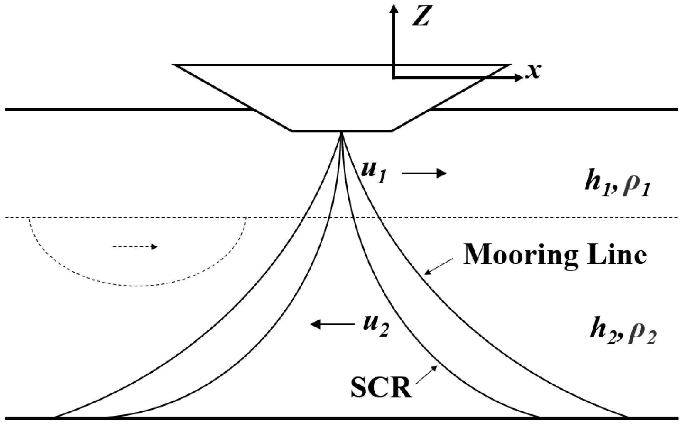
2. Model Description

As shown in Figure 1, an FPSO–SCR system comprises the FPSO, SCRs and the mooring system. The SCRs are connected to the FPSO, while the FPSO is held by the turret mooring system. Therefore, the force acting on the FPSO includes the internal solitary wave load, the restoring force of the mooring system, and the inertial fluid load. As the surface wave has little effect on the drift of the PFSO, especially in the relatively short period when the ISW pass through the FPSO, it is neglected in the present study.

In the present study, the FPSO motion equation is deduced and solved numerically with Matlab. As the restoring force of the mooring system could be easily solved based on the catenary equation, the response surface of the restoring surface to the FPSO motion is solved and incorporated into the solution of the FPSO motion. However, the responses of the SCRs are much more complicated. Therefore, the response of the riser is simulated with an FEM model in ABAQUS. As the FPSO is much larger than the riser, the riser motion has little effect on the FPSO motion; therefore, only one-way coupling is modeled in the FE model, i.e., by taking into account the FPSO motion by implementing a displacement constraint on the top end of the riser in the FEM model.

2.1. Internal Solitary Wave Equation

At present, most theories of internal solitary waves divide the flow field into two layers, with different depths and densities in each layer, and the flow directions of water particles are opposite to each other. As shown in Figure 1, each layer of fluid is assumed to be ideally incompressible and irrotational, and the upper surface of the fluid is assumed to be still, while the bottom of the water is considered an impermeable rigid wall. When the fluid is in a static equilibrium state, the height and density of the upper layer of fluid are h₁ and ρ₁, while the height and density of the lower layer are h₂ and ρ₂.

The mKdv theory is used to calculate this internal solitary wave. Although the mKdv theory requires the internal solitary wave to be weakly nonlinear, it does not need to consider the balance between dispersion and nonlinearity. It has a specified limit value for amplitude, and as long as it does not exceed this limit value, the model can be used for calculation. According to the mKdv theory, the wavefront equation of internal solitary waves can be obtained as follows:

$$\zeta ={\displaystyle \frac{{\mathrm{a} \mathrm{sech}}^2\left[\lambda \left(x-ct\right)\right]}{1-\mu { \tanh }^2\left[\lambda \left(x-ct\right)\right]}}$$

(1)

where ζ is the water particle displacement at the two-layer flow field interface, t is time, x is the position of the propagation direction of the internal solitary wave, h is the total water depth, a is the wave amplitude, λ is the characteristic wavelength, c is the phase velocity, and μ is the dispersion parameter. The λ, c and μ are deduced as follows:

$$\lambda ={\displaystyle \frac{1}{2(h-h_c)}}({\displaystyle \frac{3h{h}^{\prime }{h}^{″}}{{(h-h_c)}^3+{h_c}^3}})$$

(2)

$$c=c_0(1-{\displaystyle \frac{1}{2}}{({\displaystyle \frac{\overline{h}+a}{h-h_c}})}^2)$$

(3)

$$\mu =\left\{\begin{array}{l}{h}^{″}/h^{\prime },\overline{h}>0\\ h^{\prime }/h^{″},\overline{h}<0\end{array}\right.$$

(4)

where the intermediate variables are expressed as Equations (5)–(7):

$$h_c={\displaystyle \frac{h}{1+\sqrt{{\rho }_1/{\rho }_2}}}$$

(5)

$$\overline{h}=\left|h_2-h_c\right|, h^{\prime }=-\overline{h}-\left|\overline{h}+a\right|, h^{″}=-\overline{h}+\left|\overline{h}+a\right|$$

(6)

$$c_0=\left\{{\displaystyle \frac{gh}{2}}\left[1-{({\displaystyle \frac{4({\rho }_1-{\rho }_2)h_c(h-h_c)}{{\rho }_2{h}^2}})}^{1/2}\right]\right.{\}}^{1/2}$$

(7)

in which g is the gravitational acceleration.

The basic parameters of the selected internal solitary waves are shown in

Table 1. Internal solitary wave parameters.

Internal Solitary Waves Properties	Depth (m)	Seawater Density (kg/m3)	Wave Amplitude (m)
Upper layer fluid	274.4	1025	−90.4
Lower layer fluid	640	1028	−90.4

. The ship parameters of FPSO are shown in

Table 2. FPSO hull parameters [31].

Main Parameters of the Vessel	Symbol	Value	Unit
Production level		120,000	bpd
Storable volume		14,400	bbls
Length between perpendiculars	LBP	310	m
Molded breadth	B	47.17	m
Molded depth	H	28.04	m
Draft	T	18.9	m
Displacement of the vessel	D	240,869	mt
Center of buoyancy forward of section	FB	6.6	m
Center of gravity above base	KG	13.32	m

.

The velocity of each layer of fluid can be calculated using the following equation, while the calculation method for acceleration is obtained by taking the derivative of the following equation:

$$V=-c{\displaystyle \frac{\zeta }{h_i}}$$

(8)

where V is the fluid velocity and h_i is the depth of the desired fluid layer.

The time history curve of the fluid velocity of the internal solitary wave is shown in Figure 2. It can be seen from the figure that both the upper and lower fluids exhibit variation with time similar to a trigonometric waveform, that is, they first increase to a certain extreme value and then decrease to zero, and their period of action is relatively long, which is in line with the basic characteristics of internal solitary waves.

The time history curve of fluid acceleration for internal solitary waves is shown in Figure 3. It can be observed that the changes in acceleration and velocity are consistent, and that the value of acceleration is very small, indicating that the flow velocity in the flow field changes slowly. When the acceleration is zero, the velocity reaches its maximum value, which means that the change in fluid acceleration is consistent with the change in velocity.

2.2. Equation of the FPSO Motion

In this study, the FPSO system shown in Figure 4 is adopted for analysis. Figure 5 shows the layout of the mooring system of the FPSO. There are a total of 12 mooring lines, divided into four groups. The angle between each cable in the group is 5°, and the four groups of cables are symmetrically arranged around the FPSO.

Table 3. Mooring line parameters [31].

Name	Value	Unit
Water depth	914	m
Pre-tension	1201	kN
Mooring line quantity	4*3
Angle between three mooring lines	5	Deg
Mooring line length	2088	m
Chain stopper plate radius	7	m
First section: ground part	K4 without Block
Length	914.4	m
Diameter	88.9	mm
Dry weight	1617.1	N/m
Wet weight	1406.9	N/m
Stiffness AE	794,484	kN
Average breaking load	6512	kN
Second section: wire rope	Spiral Strand Wire
Length	1127.8	m
Diameter	88.9	mm
Dry weight	412.12	N/m
Wet weight	349.75	N/m
Stiffness AE	689,858	kN
Average breaking load	6418	kN
Third section: top part	K4 without Block
Length	45.7	m
Diameter	88.9	mm
Dry weight	1617.09	N/m
Wet weight	1406.89	N/m
Stiffness AE	794,484	kN
Average breaking load	6512	kN

shows the mooring line parameters. The mooring is a three-stage cable, with the first section being the towing bottom section, in the form of a K4 unshielded anchor chain, with a diameter of 88.9 mm, a wet weight per unit length of 1406.9 N/m, and a length of 914.4 m. The second section is the middle section, in the form of a spiral stranded polyester fiber material with a diameter of 88.9 mm, a wet weight per unit length of 349.75 N/m, and a length of 1127.8 m. The third section is the top connecting section, in the form of a K4 unsecured anchor chain, with a diameter of 88.9 mm, a wet weight per unit length of 1406.89 N/m, and a length of 45.7 m. It is shown in simplified form in Figure 6. M1 to M12 represent the 12 mooring ropes, respectively.

As shown in Figure 1, the bow direction is considered as the x positive. For a turret-moored FPSO, its longitudinal direction always aligns with the ISW direction. Taking into account the internal solitary wave load, the restoring force of the mooring system, and the inertial fluid load, the FPSO motion along the x direction is established as follows:

$$(M+M_a)∆\ddot{X}-M_a∆\ddot{\xi }=F_{xc}+F_{xr}$$

(9)

where M is the mass of the vessel, M_a is the additional mass of the vessel, $∆\ddot{X}$ is the longitudinal acceleration, and $∆\ddot{\xi }$ is the fluid acceleration. F_xc and F_xr represent the internal solitary wave load and the restoring force of the mooring system, respectively.

To solve Equation (9), the fourth-order Runge–Cutta method provided in Matlab is used; the time step size is automatically selected. As it is a classical differential equation, it is easily solved numerically. However, the key of the solution is to obtain the ISW load $F_{xc}$ and the restoring force $F_{xr}$, which is emphasized in the following parts.

2.2.1. Dragging Force of the ISW

The drag force on the FPSO is calculated using the following formula:

$$F_{xc}={\displaystyle \frac{1}{2}}{C}_{xc}\rho V^2{L}_{BP}T$$

(10)

where C_xc is the longitudinal current force coefficient, V is the fluid velocity, L_BP is the length between perpendiculars, and T is the ship’s draft. The longitudinal current force coefficient is critical to the calculation of the ISW force on the FPSO. In the present study, the suggested value from the OCIMF (Oil Companies International Marine Forum) report is adopted [32].

2.2.2. Restoring Force of the Mooring System

The fundamental reason for the generation of restoring force is due to the displacement of the FPSO, which causes changes in the horizontal and vertical forces of the cable. The relationship between the restoring force and the displacement is nonlinear and needs to be iteratively solved through the catenary equation. As shown in Figure 6, one section of the three-stage mooring line is selected for analysis.

From the catenary equation, the following can be inferred:

$$Y=(H_t/W)\left[\cosh \left({\sinh }^{-1}\tan {\theta }_t\right)-\cosh \left({\sinh }^{-1}\tan {\theta }_b\right)\right]$$

(11)

$$X=(H_t/W)\left[{\sinh }^{-1}\tan {\theta }_t-{\sinh }^{-1}\tan {\theta }_b\right]$$

(12)

$$\tan {\theta }_b=(V_t-S·W)/H_t$$

(13)

$$V_t=H_t·\tan {\theta }_t$$

(14)

where V_t and H_t are the vertical and horizontal tension at its top, V_b and H_b are the vertical and horizontal tension at its bottom, θ_t and θ_b are the top inclination angle and bottom inclination angle, S is the length of this section of cable, and W is the unit length weight of this section of cable.

From the above equation, it is easy to derive the catenary equation for the bottom section (anchor chain) when θ_b is equal to 0°:

$$Y=(H_t/W)\left[\cosh \left({\sinh }^{-1}\tan {\theta }_t\right)-1\right]$$

(15)

$$X=(H_{\mathrm{t}}/W)\left[{\sinh }^{-1}\tan {\theta }_t\right]$$

(16)

If the horizontal tension H_t at the top, vertical height Y, top inclination angle θ_t, and unit length weight W are known, then the above equation can be used to determine the following:

$$Y=(H_{\mathrm{t}}/W)\left[\cosh \left({\sinh }^{-1}\tan \theta \right)-1\right]$$

(17)

$$S=H_t\left[\tan {\theta }_t-\tan {\theta }_b\right]/W$$

(18)

Under the same conditions, the horizontal length X of the catenary can be solved by combining Equations (12), (17) and (18).

On the basis of the above catenary theory, the relationship curve between the restoring force and FPSO displacement of a specific mooring system can be solved.

Firstly, the initial state of the mooring system is solved. The mooring system of the FPSO studied in this paper has a three-stage mooring system. Generally, the initial horizontal pre-tension H₀ and initial top inclination angle θ₀ of the mooring system are known and can be calculated according to the following steps:

(1)

The initial vertical pre-tension V₀ can be calculated based on H₀ and θ₀. At this point, the middle wire part of the cable is assumed to be completely floating. The vertical force V_j and angle θ_t at the connection between the wire and the top anchor chain can be calculated.

(2)

According to the calculated V_j and θ_t, the vertical heights Y₁, Y₂ and Y₃ of the three cable segments can be solved.

(3)

The solved Y₁ + Y₂ + Y₃ is compared with the height h. If the error meets the set threshold, the next step can be taken. If not, V_j can be reasonably increased or decreased based on the positive or negative value and magnitude of the difference, and the above steps can be repeated until the difference between Y₁ + Y₂ + Y₃ and the h meets the threshold.

(4)

Then X₀, X₁, X₂, X₃ can be calculated, where X₀ is the length of the bottom support section.

(5)

After obtaining the initial conditions for the mooring line, the relationship between the restoring force and the displacement of the mooring point can be calculated. Firstly, a small uniform displacement du is assumed, and a new value of H can be determined. Then, by repeating steps (2) to (4) with the new value of H, the new X₀, X₁, X₂, X₃ values can be calculated.

(6)

After obtaining the new values for X₀, X₁, X₂, X₃, their sum can be subtracted from the result obtained in step (4), and the difference can be compared with the set threshold. If it meets the requirement, the following steps can be performed. If it does not meet the requirement, H can be slightly adjusted by the difference, and step (5) can be repeated until the difference meets the threshold.

After obtaining the value of H corresponding to the small displacement du, du can be slowly and uniformly increased, and steps (5) to (6) can be repeated to obtain the corresponding H; thus, the correspondence between the horizontal tension of a mooring point and its displacement can be obtained.

Based on the above theory, specific three-stage or multi-stage catenary mooring systems can be calculated and analyzed.

The bow of the FPSO is assumed to be moving in the direction of the M2 mooring line. The calculation method for the restoring force of the M8 and M2 mooring lines can be directly used as described above, while the restoring force of the other mooring lines needs to be modified to a certain extent. The changes in restoring force of the M1, M3, M7, and M9 mooring lines can be calculated through simple geometric substitution. The restoring force of the remaining six root cables can be solved through simple coordinate transformation, and the calculation method is as follows:

$$F_r=(2\ast \cos 5^{\circ }+1){\sin }^2\beta ({\displaystyle \sum F_{ri}}+{\displaystyle \sum F_{rj}})$$

(19)

where F_r is the total restoring force of the mooring system, F_ri is the restoring force of a single mooring line away from the FPSO, F_rj is the restoring force of a single mooring line close to the FPSO, and β is the angle between the M2 mooring line and the bow direction of the FPSO.

The variation in the total restoring force of the mooring system after solving is shown in Figure 7. It can be seen that the magnitude of the total restoring force is positively correlated with the displacement of the FPSO. Compared to the work of Wichers and Devlin (2001) [31], the solution of the restoring shows very good agreement.

2.3. FEM Model of the Coupled FPSO–SCR System

The response of the SCR is simulated in ABAQUS. As shown in Figure 8, the FEM model comprises two parts, i.e., the SCR and the seabed. As the soil–pipe interaction is not of interest in the present study, the seabed is considered as a rigid flat surface. Therefore, the soil–pipe interaction is considered as rigid contact, and a friction coefficient of 0.2 is assumed between the seabed and the SCR. The SCR has a diameter of 0.4064 m (16 inch), and a thickness of 0.0254 m (1 inch). The SCR geometry is initially modeled according to the solution of the catenary equation. And then the gravity is implemented on the SCR. The number of mesh grids in this model is 467,342. The number of grid nodes directly affects the iterative equations and the accuracy and convergence speed of the calculation model. If the number of mesh nodes is too small, the accuracy of the calculation result is low. If the number of mesh nodes is too large, the number of iteration steps and convergence time increases. Therefore, through the verification of grid sensitivity (as shown in

Table 4. Grid sensitivity analysis.

Number of Grid Nodes	Maximum Stress	Deviation
89,543	129 MPa	-
203,537	138 MPa	9 MPa
391,352	144 MPa	6 MPa
467,342	148 MPa	4 MPa
503,456	149 MPa	1 MPa

), for this model, when the grid nodes are greater than 467,342, the deviation of maximum stress is very small, and it can be concluded that the number of grid nodes has little impact on the simulation results. The initial geometry of the SCR in the equilibrium position is shown in Figure 8. The maximum stress in the SCR is at the top end of the SCR, which is caused by its self-gravity.

SCR is a type of catenary. The equation of a catenary can be derived through differential equations. By representing the arc length of the chain as a function of the position of the particle on the catenary, the parametric equation of the catenary can be obtained. When the tangent slope of the catenary at the origin is 0, the standard equation of the catenary is as follows:

$$y={\displaystyle \frac{T}{g\rho }}\left(\cosh \left({\displaystyle \frac{g\rho }{T}}x\right)-1\right)$$

(20)

The standard equation for a catenary with an angle at the origin is as follows [33]:

$$y={\displaystyle \frac{T}{g\rho }}\cosh \left({\displaystyle \frac{g\rho }{T}}x+\ln \left(\tan \alpha +\sec \alpha \right)\right)-{\displaystyle \frac{T}{g\rho }}\sec \alpha$$

(21)

where T is the horizontal pulling force to the left at the lowest point, and ρ is the mass per unit length of the iron chain.

Given the water depth h and initial angle θ of the SCR, the relevant catenary theory can be used to derive the following:

$$\left\{\begin{array}{c}y=a\left(\cosh {\displaystyle \frac{x}{a}}-1\right)\\ {\displaystyle \frac{x}{a}}={\sinh }^{-1}\tan \theta \\ h=a\cosh {\sinh }^{-1}\tan \theta -a\end{array}\right.$$

(22)

Table 5. SCR parameters [31].

Calculated Parameters	Value	Unit
Water depth	914.4	m
Angle between the top and the water surface	60	°
Outer diameter of riser	0.4064	m
Inner diameter of riser	0.3556	m
Poisson’s ratio	0.3
Young’s modulus	2.1 × 105	MPa
Quality density	7850	kg/m
Total length of pipeline	2085	m
Dragging section length	500	m
Horizontal tension	8220.5	N

provides detailed parameters of the selected SCR. Figure 9 shows the form of the catenary equation corresponding to the SCR riser, which is the approximate static equilibrium form of the riser without considering fluid loads.

3. Results and Discussion

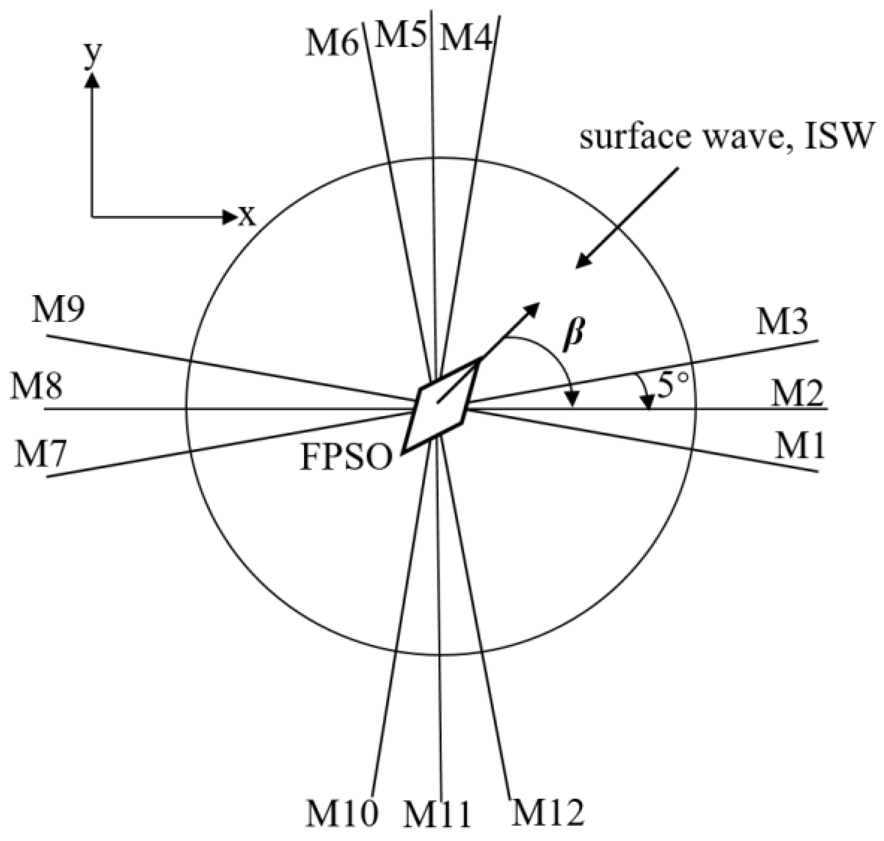
3.1. FPSO Motion Response and Influence of Mooring Pre-Tension on FPSO Motion

The horizontal displacement time history and horizontal velocity time history of an FPSO under three different pre-tensions are shown in Figure 10 and Figure 11. It can be clearly seen from the figures that a positive displacement peak appears around 2000 s when the fluid flow velocity reaches its maximum value. This is due to the effect of internal solitary waves. Then, as the fluid flow velocity decreases, the FPSO moves towards the equilibrium position under the restoring force of the mooring line. After returning to the equilibrium position, it begins to move in the opposite direction. After losing the effect of internal solitary waves, it undergoes harmonic motion with gradually decreasing displacement amplitude under the influence of fluid resistance and additional mass force. It can be clearly seen that, under the action of internal solitary waves, the FPSO experiences significant horizontal displacement. By analyzing the velocity image, it can be concluded that the overall velocity of FPSO under the action of internal solitary waves is not significant, but its changes are very complex. When changing the horizontal pre-tension, the displacement time history curve of the FPSO undergoes significant changes. As the horizontal pre-tension decreases, the displacement of the FPSO increases significantly at the same time. At the same time, the occurrence time of the FPSO displacement amplitude also lags behind the decrease in horizontal pre-tension. The main reason for this phenomenon is that, due to the unchanged internal solitary wave load, it takes more time for the cable recovery force to reach equilibrium with the internal solitary wave load. The smaller the pre-tension, the larger the peak velocity, which is also related to the longer time required for the cable recovery force to balance with the internal solitary wave load.

Figure 12 shows the time history curve of the internal solitary wave load. The internal solitary wave load reaches its maximum value before 2000 s, and the displacement reaches its maximum value around 2000 s, which is consistent with the actual situation.

3.2. Influence of Mooring Line Distribution on FPSO Motion

In the previous analysis, due to the constant propagation direction of internal solitary waves, the influence of the cable distribution on FPSO displacement cannot be intuitively observed. Therefore, the angle between the internal solitary waves and the hull is set to 0°, and the angle between the bow and M2 cable is changed to achieve a relative change in the direction of internal solitary waves with respect to the cable. Due to the symmetrical arrangement of the selected mooring lines modeled in this article, the motion characteristics of the FPSO can be analyzed by selecting angles of 0°, 15°, 30°, and 45° between the bow of the ship and the M2 mooring line, where β is the angle between the bow of the ship and the M2 mooring line.

As shown in Figure 13, it can be seen that with the increase in angle, the horizontal displacement time history of FPSO changes to a certain extent and its displacement amplitude become smaller, while the appearance of displacement amplitude is relatively earlier. The reason is that, as the angle increases, the utilization rate of the mooring line by the FPSO increases. For example, when the angle between the bow of the ship and the M2 mooring line is 0° propagation, only one mooring line is preventing the displacement of the FPSO at 0 s. As the displacement increases, the two adjacent mooring lines begin to participate. If the bow of the ship forms a 45° angle with the M2 mooring line, two mooring lines will directly participate at 0 s. Although the effect of a single mooring line on preventing FPSO displacement may be weakened due to the angle, the combined effect of the two mooring lines is stronger. As shown in Figure 14, the change in speed is relatively insignificant.

3.3. Tension Characteristics of Mooring Lines

The mooring system, as an important component of the FPSO, cannot ignore the changes in tension caused by the displacement of the FPSO in its mooring lines. The tension characteristics of the middle mooring lines in each group, namely M2, M5, M8, and M11, are analyzed. The bow of the FPSO is selected to form a 15° angle with the M2 mooring line, in order to highlight the changes in tension of each mooring line and analyze the tension characteristics of different mooring lines.

Figure 15 shows the time history curves of tension changes in cables M2, M5, M8, and M11. The tension changes in the cables also exhibit a certain periodicity, and the amplitude of the changes appears during the time of the internal solitary wave action. Comparing the tension changes of the four cables, it is found that the tension change of the M8 cable is more significant than that of the M2 cable. The change of the M5 cable is the least significant, as it is both close to the FPSO and is less affected by angles.

Taking the M8 mooring line as an example, the angle between the bow of the ship and the M2 mooring line is changed, and the influence of different mooring line arrangements on the tension characteristics of the mooring line is analyzed. Figure 16 shows the time history of tension changes in the FPSO under different incident angles of internal solitary waves. It can be seen that, after changing the angle from 0° to other angles, the peak tension change of the mooring line significantly decreases, which is due to the improved utilization rate of the mooring line.

3.4. Influence of FPSO Motion on SCR Dynamic Response

Figure 17 shows the stress envelope of the SCR under the floating body motion. When the ISW crest reach the FPSO position, i.e., t ≈ 2000 s, the stress data curve of the SCR reaches its maximum value.

In order to more intuitively find the trend of SCR stress in dynamic characteristic analysis over time, a key node at the touch-down region is selected to output the stress over time, which is a node located at a distance of approximately 1250 m along the SCR direction. Figure 18 shows the stress history data of the selected node under different floating body motion conditions. In the absence of floating body motion and surface wave action, the SCR is only affected by internal solitary waves. The maximum stress value is about 87.3 MPa when the combined effects of internal solitary wave velocity and acceleration are at a maximum, and the minimum stress value is about 83.8 MPa when the combined effects of internal solitary wave velocity and acceleration are at a minimum. When the corresponding floating body motion and surface wave action are added, the curve trajectories of the two cases are basically the same, and are similar to the top floating body motion trajectory curve. In addition, after adding surface waves, the process curve fluctuates continuously up and down with the fluctuation in surface waves. When the top floating body motion reaches its maximum (t ≈ 2000 s), there is a maximum stress value of about 104.3 MPa, and when the top floating body motion reaches its minimum (t = 2800 s), there is a minimum stress value of about 79.6 MPa.

Figure 19 shows the maximum displacement time data for the corresponding effects of floating body motion with surface waves and floating body motion without surface waves. The sizes of the two are almost the same, but there is a slight difference in the occurrence time, which is t = 2084 s and t = 2072 s, respectively. In other words, the presence of surface waves causes the maximum displacement of the SCR to appear earlier, but the addition of surface waves does not produce a significant dynamic response in the SCR, which is attributed to the SCR’s ability to handle deep and large movements of the top floating body.

3.5. Influence of ISW Incident Angle on SCR Dynamic Response

Figure 20, Figure 21, Figure 22 and Figure 23 show the stress envelope diagrams of SRC for inflow angles of 0°, 30°, 60°, and 90°, respectively. By observing the stress curve at each moment, it is ultimately found that the stress values at various inflow angles reached their maximum at times around t = 2000 s.

As the inflow angle increases, the stress value of the SCR slightly decreases, and the specific comparison data are shown in Figure 24. The main reason may be that, when the incoming direction of the internal solitary wave is consistent with the SCR arrangement direction, stress concentration is easily generated, and when the internal solitary wave propagates laterally, a portion of the stress concentration is released.

Figure 25 shows the maximum displacement time values at different inflow angles. By comparing the displacement of the SCR in different inflow directions, it is found that there is no certain linear relationship between inflow angle and SCR displacement in the range of 0°~90° inflow directions, and there is not much change in displacement under the four different inflow angles.

4. Conclusions

(1)

The velocity of the FPSO under the action of internal solitary waves is generally not large, but its variation is very complex. The internal solitary wave load reaches its maximum value before the ISW crest reaches the FPSO, but the FPSO displacement reaches a maximum when it reaches the FPS, which is consistent with the actual situation.

(2)

The smaller the horizontal pre-tension of the mooring cable, the greater the displacement of the FPSO, and the more time needed for the FPSO displacement to decay. The arrangement of mooring lines also has a significant impact on the FPSO. For symmetrically arranged mooring systems, the larger the angle between the internal solitary waves and the mooring lines, the smaller the horizontal displacement of the FPSO.

(3)

Considering both the motion of the FPSO and the internal solitary waves, the stress of the SRC reaches its maximum value when the FPSO reaches its maximum motion, while it reaches its minimum value when the FPSO reaches its minimum motion.

(4)

When the ISW crest reaches the FPSO, the stress values of the SCR at the four incident angles of 0°, 30°, 60°, and 90° all reach their maximum. As the incident angle increases, the stress value of the SCR slightly decreases.

References

1. Zheng, Y.D.; Lin, J.; Chen, X. Application of fluctuations in the sound field in inversion of internal solitary wave phase speed. Ocean Eng. 2024, 305, 117878. [Google Scholar] [CrossRef]
2. Li, R.J.; Li, M. Generation and evolution of internal solitary waves in a coastal plain estuary. J. Phys. Oceanogr. 2024, 54, 641–652. [Google Scholar] [CrossRef]
3. Cheng, L.; Wang, C.; Guo, B.B.; Liang, Q.Y.; Xie, Z.L.; Yuan, Z.M.; Chen, X.P.; Hu, H.B.; Du, P. Numerical investigation on the interaction between large-scale continuously stratified internal solitary wave and moving submersible. Appl. Ocean Res. 2024, 145, 103938. [Google Scholar] [CrossRef]
4. Zhang, X.D.; Li, X.F. Unveiling three-dimensional sea surface signatures caused by internal solitary waves: Insights from the surface water ocean topography mission. J. Oceanol. Limnol. 2024, 42, 709–714. [Google Scholar] [CrossRef]
5. Sun, H.W.; You, Y.X.; Lei, J.R. Deflection and drag on flexible marine structures in steady currents and internal solitary waves. Phys. Fluids 2024, 36, 106603. [Google Scholar] [CrossRef]
6. Yu, J.X.; Liu, X.W.; Sun, B.; Yu, Y.; Wu, S.B.; Li, Z.M. Nonlinear dynamic response of touchdown zone for steel catenary riser under multiple internal solitary waves. Ocean Eng. 2024, 297, 117141. [Google Scholar] [CrossRef]
7. Guo, Y.L.; Li, Q.; Chen, X.; Peng, J.H.; He, X. Dynamic analysis on the interaction of two successive internal solitary waves with a ridge. Phys. Fluids 2024, 36, 066612. [Google Scholar] [CrossRef]
8. Adim, M.; Bianchini, R.; Duchene, V. Relaxing the sharp density stratification and columnar motion assumptions in layered shallow water systems. Comptes Rendus Math. 2024, 362, 1597–1626. [Google Scholar] [CrossRef]
9. Qiu, N.; Liu, X.Q.; Liu, Z.W.; Li, Y.W.; Hu, P.J.; Chang, Y.J.; Chen, G.M. Mechanical model and characteristics of deep-water drilling riser-wellhead system under internal solitary waves. Mar. Struct. 2023, 90, 103439. [Google Scholar] [CrossRef]
10. Lin, Z.H. Numerical study on the forces and moments on a bottom-mounted cylinder by internal solitary wave. J. Fluids Struct. 2023, 121, 103952. [Google Scholar] [CrossRef]
11. Makarenko, N.I.; Maltseva, J.L.; Cherevko, A.A. Solitary Waves in a Two-Layer Fluid with Piecewise Exponential Stratification. Fluid Dyn. 2023, 58, 1235–1245. [Google Scholar] [CrossRef]
12. Li, Z.X.; Wang, J.; Lu, Y.G.; Huang, S.S.; Yang, Z. Propagation speed model of mode-2 internal solitary waves in the northern South China Sea based on multi-source optical remote sensing. Ocean Eng. 2024, 315, 119850. [Google Scholar] [CrossRef]
13. Qiu, N.; Liu, X.Q.; Li, Y.W.; Hu, P.J.; Chang, Y.J.; Chen, G.M.; Meng, H.X. Dynamic catastrophe analysis of deepwater mooring platform/riser/ wellhead coupled system under ISW. Reliab. Eng. Syst. Saf. 2024, 246, 110084. [Google Scholar] [CrossRef]
14. Yilmaz, E.U.; Khodad, F.S.; Ozkan, Y.S.; Abazari, R.; Abouelregal, A.E.; Shaayesteh, M.T.; Rezazadeh, H.; Ahmad, H. Manakov model of coupled NLS equation and its optical soliton solutions. J. Ocean Eng. Sci. 2024, 9, 364–372. [Google Scholar] [CrossRef]
15. Chang, Z.; Sun, L.N.; Liu, T.F.; Zhang, M.; Liang, K.D.; Meng, J.M.; Wang, J. Experimental study on the variation of optical remote sensing imaging characteristics of internal solitary waves with wind speed. J. Oceanol. Limnol. 2024, 42, 408–420. [Google Scholar] [CrossRef]
16. Koop, C.G.; Butler, G. An investigation of internal solitary waves in a two-fluid system. J. Fluid Mech. 1981, 112, 225–251. [Google Scholar] [CrossRef]
17. Segur, H.; Hammack, J.L. Soliton models of long internal waves. J. Fluid Mech. 1982, 118, 285–304. [Google Scholar] [CrossRef]
18. Michallet, H.; Barthelemy, E. Experimental study of interfacial solitary waves. J. Fluid Mech. 1998, 366, 159–177. [Google Scholar] [CrossRef]
19. Grue, J.; Jensen, A.; Russ, P.O.; Sveen, J.K. Properties of large-amplitude internal waves. J. Fluid Mech. 1999, 380, 257–278. [Google Scholar] [CrossRef]
20. Brandt, P.; Rubino, A.; Alpers, W.; Backhaus, J.O. Internal waves in the Strait of Messina studied by a numerical model and synthetic aperture radar images from the ERS 1/2 satellites. J. Phys. Oceanogr. 1997, 27, 648–663. [Google Scholar] [CrossRef]
21. Huang, W.H.; You, Y.X.; Wang, X.; Hu, T.Q. Experimental study and theoretical model of internal solitary wave generation in finite depth two-layer fluid. Acta Phys. Sin. 2013, 62, 354–367. [Google Scholar] [CrossRef]
22. Liu, A.K. Analysis of nonlinear internal waves in the New York Bight. J. Geophys. Res. Ocean. 1988, 93, 12317–12329. [Google Scholar] [CrossRef]
23. Cai, S.Q.; Long, X.M.; Gan, Z.J. A method to estimate the forces exerted by internal solitons on cylindrical piles. Ocean Eng. 2003, 30, 673–689. [Google Scholar] [CrossRef]
24. Liu, B.T. The Numerical Simulation of the Interaction of Internal Solitary Waves with the Deep-Sea Riser. Master’s Thesis, Shanghai Jiao Tong University, Shanghai, China, 2011. [Google Scholar]
25. Xu, Z.H. The Interaction Characteristics of Internal Solitary Waves with Floating Production Storage and Offloading System. Master’s Thesis, Shanghai Jiao Tong University, Shanghai, China, 2014. [Google Scholar]
26. Ren, Y.P.; Tian, H.; Chen, Z.Y.; Xu, G.H.; Liu, L.J.; Li, Y.B. Two kinds of waves causing the resuspension of deep-sea sediments: Excitation and internal solitary waves. J. Ocean Univ. China 2023, 22, 429–440. [Google Scholar] [CrossRef]
27. Huang, M.M.; Gao, C.J.; Zhang, N. Numerical research on hydrodynamic characteristics and influence factors of underwater vehicle in internal solitary waves. Int. J. Offshore Polar Eng. 2023, 33, 27–35. [Google Scholar] [CrossRef]
28. Zhang, B.B.; Zhang, T.Y.; Duan, W.Y.; Wang, Z.; Guo, X.Y.; Hayatdavoodi, M.; Ertekin, R.C. Internal solitary waves generated by a moving bottom disturbance. J. Fluid Mech. 2023, 963, 32. [Google Scholar] [CrossRef]
29. Li, F.H.; Guo, H.Y.; Gu, H.L.; Liu, Z.; Li, X.M. Deformation and stress analysis of the deepwater steel lazy wave riser subjected to internal solitary waves. J. Ocean Univ. China 2023, 22, 377–392. [Google Scholar] [CrossRef]
30. Tan, D.L.; Wang, X.; Duan, J.L.; Zhou, J.F. Linear analysis of the dynamic response of a riser subject to internal solitary waves. Appl. Math. Mech.-Engl. Ed. 2023, 44, 1023–1034. [Google Scholar] [CrossRef]
31. Wichers, J.E.W.; Devlin, P.V. Effect of coupling of mooring lines and risers on the design values for a turret moored FPSO in deep water of the Gulf of Mexico. In Proceedings of the ISOPE International Ocean and Polar Engineering Conference, Stavanger, Norway, 17 June 2001. [Google Scholar]
32. OCIMF. Prediction of Wind and Current Loads on VLCCs; Oil Companies International Marine Forum: London, UK, 1977. [Google Scholar]
33. Zhang, H.J.; Yi, H.R.; Wang, H.; Liang, J.L. The derivation and application of the catenary equation. Technol. Innov. Appl. 2019, 26, 173–176. [Google Scholar] [CrossRef]
Figure 1. Schematic diagram of internal solitary wave model.
Jmse 13 00521 g001
Figure 2. Time history curve of fluid flow velocity.
Jmse 13 00521 g002
Figure 3. Time history curve of fluid acceleration.
Jmse 13 00521 g003
Figure 4. Three-dimensional cable layout of the inner turret mooring system.
Jmse 13 00521 g004
Figure 5. Projection of mooring rope layout.
Jmse 13 00521 g005
Figure 6. A certain section of the cable.
Jmse 13 00521 g006
Figure 7. Changes in total restoring force of mooring system.
Jmse 13 00521 g007
Figure 8. FEM model of the SCR.
Jmse 13 00521 g008
Figure 9. The form of the catenary equation corresponding to the SCR riser.
Jmse 13 00521 g009
Figure 10. Displacement time history of FPSO under different pre-tension conditions.
Jmse 13 00521 g010
Figure 11. Speed time history of FPSO under different pre-tension conditions.
Jmse 13 00521 g011
Figure 12. Time history curve of the internal solitary wave load.
Jmse 13 00521 g012
Figure 13. Time history of horizontal displacement of FPSO under different incident angles of internal solitary waves.
Jmse 13 00521 g013
Figure 14. Time history of FPSO velocity under different incident angles of internal solitary waves.
Jmse 13 00521 g014
Figure 15. Time history curves of tension changes in cables M2, M5, M8, and M11.
Jmse 13 00521 g015
Figure 16. Time history of tension changes in FPSO under different incident angles of internal solitary waves.
Jmse 13 00521 g016
Figure 17. The stress envelope of the SCR under floating body motion.
Jmse 13 00521 g017
Figure 18. Stress history data of selected nodes under different floating body motion conditions.
Jmse 13 00521 g018
Figure 19. The effect of surface waves on displacement.
Jmse 13 00521 g019
Figure 20. Stress envelope diagram when the inflow angle is 0°.
Jmse 13 00521 g020
Figure 21. Stress envelope diagram at an inflow angle of 30°.
Jmse 13 00521 g021
Figure 22. Stress envelope diagram at an inflow angle of 60°.
Jmse 13 00521 g022
Figure 23. Stress envelope diagram at a flow angle of 90°.
Jmse 13 00521 g023
Figure 24. Maximum stress values at different inflow angles.
Jmse 13 00521 g024
Figure 25. Maximum displacement time values at different inflow angles.
Jmse 13 00521 g025