Article

Fatigue Life Prediction of Submarine Pipelines with Varying Span Length and Position

1
Haikou Sub-Bureau of Guangzhou Bureau, EHV Transmission Company of China Southern Power Grid Co., Ltd., Haikou 570216, China
2
State Key Laboratory of Coastal and Offshore Engineering, Dalian University of Technology, Dalian 116024, China
*
Author to whom correspondence should be addressed.
J. Mar. Sci. Eng. 2025, 13(4), 763; https://doi.org/10.3390/jmse13040763
Submission received: 16 March 2025 / Revised: 6 April 2025 / Accepted: 8 April 2025 / Published: 11 April 2025
(This article belongs to the Special Issue Advanced Research in Flexible Riser and Pipelines)

Abstract

:
Free spans of submarine pipelines are prone to be subjected to vortex-induced vibration (VIV) under the action of currents, leading to fatigue damage of submarine pipelines. In the traditional method, the fatigue damage is predicted assuming that the length of free span is a constant. However, the free-span length may vary in time and space due to local scour and sand wave migration in engineering practice. This study proposed probabilistic methods to predict the fatigue life of the free spans by considering the effect of variant span length and span position. Truncated Gaussian, Raileigh and Uniform distributions of span length due to local scour, and a sinusoidal pattern with a constant migration rate is assumed for the sand wave due to the lack of field scan data. The fatigue life of a 120 m long span under a constant current-induced flow with the velocity of 0.7 m/s has been assessed. Results show that comparing with the fatigue life of a fixed span, the present method leads to an increase in the fatigue life by about ten times.

1. Introduction

Submarine pipelines are widely used to transport oil and gas in ocean engineering. Free spans might form due to the local scour, sand wave migration, etc. When the currents flow through the free-spanning pipelines, periodic displacement responses will occur if VIV happens. VIV might lead to the fatigue failure of submarine pipelines, causing severe economic losses and environmental disasters.
Many studies have focused on the fatigue failure of free-spanning pipelines. Kapurial et al. [1] studied the fatigue failure problem caused by the cross-flow VIV of free-spanning pipelines supported on semi-infinite elastic soil seabed at the ends and gave the formula for calculating the fatigue damage of pipelines under the combined action of waves and currents. Fyrileiv and Mørk [2] studied the dynamic responses of the free-spanning pipelines based on the Euler–Bernoulli beam theory and predicted the fatigue life of the pipelines under different boundary conditions. Gamino [3] used the Euler–Lagrange coupling method to simulate the interaction between pipelines and seabed. There are many seabed—pipeline interaction models used to predict the VIV, and accurate prediction of VIV is necessary to reasonably predict the fatigue life of submarine pipelines. The realistic model is the nonlinear model due to the varying seabed contact. Ulveseter et al. [4] used the time domain model to calculate the cross-flow VIV and used discrete dampers and springs to model the seabed–pipeline contact. The fatigue analysis of the pipelines is affected not only by the seabed–pipeline interaction, there are many other factors that can also affect the fatigue analysis. Yttervik et al. [5] analyzed the influence of current velocity and direction on the fatigue failure of submarine pipelines. Esplin and Stappenbelt [6] evaluated the maximum allowable span length and fatigue damage characteristics of the submarine pipeline through the S-N curve. Gazis [7] presented a Monte Carlo simulation methodology for a reliability assessment of free-spanning pipeline systems subjected to random waves. Dong et al. [8] calculated the fatigue life under different span lengths using a finite element numerical model.
Numerous factors influence pipeline fatigue, and the seabed environment is intricate, jointly contributing to significant uncertainties in submarine pipeline fatigue. The fatigue of submarine pipelines has great uncertainty. Therefore, some studies have analyzed the fatigue reliability of pipelines from the perspective of probability. Palmer [9] discussed the definition of failure probabilities in pipeline reliability analysis. Shabani et al. [10] used the theory of Probability of Failure (POF) to estimate the reliability of free-spanning submarine pipelines. They used the Monte Carlo method to calculate the POF of pipelines with different ratios of span length to pipeline diameter. Shabani et al. [11] used Finite-Element Reliability based on the Artificial Neural Network method to evaluate the fatigue probability of free-spanning pipelines. Monte Carlo Sampling was used to optimize the Artificial Neural Network to obtain the POF, which was used to evaluate the fatigue reliability level. They also investigated the effect of different span lengths and operating pressure on POF. Li et al. [12] considered the dynamic characteristics and uncertainties of free-spanning submarine pipeline fatigue failure. The Dynamic Bayesian Network was used to model dynamic fatigue failure scenarios. And then, analyzing the dynamic probability of pipeline fatigue failure, the time-dependent occurrence probability of fatigue failure causes is obtained. The above probabilistic analysis used the Monte Carlo method, which requires considerable work.
The above research on pipeline fatigue was based on fixed free span. However, engineering investigations confirm that free-spanning pipelines are dynamic because of local scour or sand waves. Some pipelines may be re-buried by the transported sediment or may continue to be eroded by the current to form a longer span (Pinna et al. [13]). With the movement of sand waves, the original free span is buried, and a new free span is simultaneously formed at both ends of the sand wave (Pu et al. [14]). This study considers the varying span length and position due to the local scour and sand wave migration, respectively. The fatigue life of the pipeline is predicted from the perspective of probability. The proposed method can quickly solve the fatigue life’s PDF under the various PDF of span length. More field or experimental data related to the damage determined from pipeline monitoring (c.f., Worden et al. [15], West et al. [16], Ceravolo et al. [17]) are helpful to improve the accuracy and robustness of the proposed model.
The rest of this study is organized as follows: The numerical model used in this study is briefly introduced in Section 2. Then, the numerical model is validated by considering the VIV response of a free span. Section 3 investigates the PDF of the fatigue life of the pipeline under varying span lengths due to local scour, and then the fatigue life of the free-spanning pipeline in the situation where the suspension position changes due to sand wave migration is predicted; Finally, conclusions are drawn in Section 4.

2. Numerical Model

In the present study, a time domain numerical model, proposed by Ulveseter et al. [4], is employed to estimate the cross-flow VIV dynamic response of the free span due to local scour. The sketch of the formation of the free span is shown in Figure 1. The sketch of the formation of free span due to local scour. The coordinate origin locates at the leftmost side of the pipeline. The x-axis is along the axis of the pipeline and the y-axis is perpendicular to the seabed. Two parts of the pipeline contacting with the seabed are defined as the span shoulder, with their lengths (Ls) both 130 m. The starting point of the free span is 130 m away from the coordinate origin, and the total length of the span (L) is 120 m.
In the present study, the pipeline is idealized as an Euler–Bernoulli beam. The governing equation for the oscillation of the free span subjects to VIV is:
E I 4 u y x 4 N 2 u y x 2 + C u y t + m p 2 u y t 2 = f ( x , t )
where EI is the bending stiffness, N is the pretension in the pipeline, C is the total damping, including the soil damping and structural damping, uy is the displacement of the pipeline in the y direction, mp is the specific mass per unit length, and f (x, t) is the hydrodynamic force on the pipeline.
In the present study, the governing Equation (1) is solved by the finite element method. The finite element method is used to discretize Equation (1) using the Hermit interpolation function. The dynamic response of the free span can be obtained by solving the following dynamic equilibrium equation:
M s ¨ ( t ) + ( C s + C b ) s ˙ ( t ) + ( K s + K b ) s ( t ) = F y
where M is the consistent mass matrix including added mass, Cs and Cb are the structural damping matrix and the soil damping matrix, Ks and Kb are the structural stiffness matrix and the soil stiffness matrix, s(t) is the response displacement of the pipeline, and Fy is the hydrodynamic force from Thorsen’s model (Thorsen et al. [18]). A Rayleigh-damping, Cs = α1M + α2Ks, is employed to model the structural damping with α1 = 1.18 and α2 = 1.42 × 10⁻⁴ as proposed by Thorsen et al. [18].
The pipeline is idealized as an assembly of a set of beam elements. Each element involves four degrees of freedom, including one cross-flow translation and one rotation at each end. Employing the Hermit shape function, the element mass matrix me and the element structural stiffness matrix ks are illustrated by Equations (3) and (4), respectively.
m e = m 420 156 22 l 22 l 4 l 2 54 13 l 13 l 3 l 2 54 13 l 13 l 3 l 2 156 22 l 22 l 4 l 2
k s = E I l 3 12 6 l 6 l 4 l 2 12 6 l 6 l 2 l 2 12 6 l 6 l 2 l 2 12 6 l 6 l 4 l 2 + N 30 l 36 3 l 3 l 4 l 2 36 3 l 3 l l 2 36 3 l 3 l l 2 36 3 l 3 l 4 l 2
where m is the sum of specific mass and added mass per unit length, and l is the element length.
Complex contact between the pipeline and the surrounding seabed can occur when VIV takes place, and significant changes in the contact region are possible including separation and recontact, hence a nonlinear seabed–pipeline contact model is introduced as shown in Figure 2. The seabed–pipeline interaction is piecewise nonlinear, which is modeled as a series of discrete soil dampers and soil springs. Nonlinear seabed–pipeline interaction analysis requires the update of the stiffness matrix and damping matrix for each time step during time integration. The vertical soil stiffness kb = 40,000 N/m, at each time step, using the information associated with the seabed position and the pipeline displacement to check whether the pipeline is in contact with the seabed. If there is contact, the value of stiffness and damping is added. If there is no contact, we check the next node along the pipeline without adding stiffness and damping terms (Ulveseter et al. [4]).
The hydrodynamic force perpendicular to the incoming flow direction consists of the added mass term, the excitation force term, and the hydrodynamic damping term (Thorsen et al. [18]):
F y = ρ π D 2 4 s ¨ + 1 2 ρ D U 2 C v cos ( φ e x c , y ) 1 2 ρ D C d , y s ˙ s ˙
where Cv is an empirical coefficient for amplitude-dependent force (Thorsen et al. [18], Figure 2), which is a function of the displacement amplitude ratio s0/D determined from the empirical database used in the frequency-domain model for predicting the VIV response (Passano et al. [19]), φexc,y = 2πfst + θ is the instantaneous phase of Fy with fs = StU/D being the vortex shedding frequency, where St ≈ 0.2 is the Strouhal number (Summer [20]), θ is the initial phase at t = 0, and Cd,y = 0.31 + 0.89 s0/D. It worth noting that the wall-proximity effect has not been considered by Thorsen’s hydrodynamic model. For spans with the gap ratio e/D < 1, adopting this model will overestimate the fatigue damage, because the vortex shedding will be noticeably suppressed when the pipeline gets closer to the wall.
The model parameters of the mentioned numerical model are listed in Table 1.
Using Newmark-β time integration, the response cross-flow displacement along the axis of the free span (x-axis) is calculated. Then, the stress is obtained according to the following relationship:
σ = D s x x 2 E
where sxx is the second derivative of the response.
Figure 3 and Figure 4 show the simulated response amplitude ratio s0/D and stress amplitude σa comparisons among the present numerical model, the nonlinear model of seabed–pipeline interaction developed by Ulveseter et al. [4], and the linear model in VIVANA, respectively. The present results agree well with those predicted by Ulveseter et al. [4]. However, the results derived from the VIVANA give a much larger response and stress because the linear model in VIVANV cannot consider the nonlinear contact between the pipeline and the seabed.
The rainflow counting method is used for the stress statistics to obtain the number of stress cycles ni under the i-th order stress. From the S-N curve, under the stress range Si, the predicted number of failure cycles Ni can be obtained. Noting that the S-N curve is suitable for the zero-mean stress case, which cannot be directly used in this study. For handling the non-zero mean stress, an additional equation σar = f (σa, σm) is needed to modify the stress (Dowling et al. [21]):
σ a r = σ a σ max
where σm is the mean stress, and σmax = σa + σm is the maximum stress.
The fatigue damage of a submarine pipeline is calculated by Miner’s linear damage accumulation rule (Palmgren [22]; Miner [23]).
D f = n i N i
where 1 < Df < 0 is the cumulative fatigue damage.
When the variable of the cumulative fatigue damage Df is obtained, the fatigue damage over one year can be calculated as:
D a = D f × t s / ( Δ t × t 1 )
where ts = 3600 × 24 × 365 is the number of seconds in a year, Δt is the time interval, t1 is the time history measured by the rain flow method. The fatigue life of the pipeline can be calculated as:
T = 1 D a
The result of the fatigue damage of the pipeline over one year is shown in Figure 5. It can be seen from Figure 5 that from the starting point of the span, the pipeline begins to have fatigue damage, and the largest fatigue damage is found at 190 m, near the mid-span. Its fatigue damage is 0.00563 1/year, and the predicted fatigue life of the pipeline is about 177 years.

3. Numerical Results

3.1. Fatigue Life Analysis of the Pipeline Under Varying Span Length Due to Local Scour

When the pipeline is installed on the seabed, the current may erode the seabed to form larger spans. With the increase in the span length, the pipeline will gradually sag. Eventually, the center of the spanning section of the pipeline will contact with the seabed again, and the soil will accrete around the touchdown section, forming a new span. The burial and suspension caused by the scouring are dynamic, so the span length varies with time.
For investigating the fatigue failure of the pipeline under varying free spans, the model introduced in Section 2 is chosen. The parameters are shown in Table 1. The span length caused by the local scour varies from 0 to Lmax. The maximum span length Lmax is defined as the pipeline deflecting one diameter (Leckie et al. [24]), which is estimated according to:
L max = ( 384 D E I 3 ω o p ) 1 4 = 120   m
where ωop is the submerged weight per unit pipeline length.
The varying span length L can be described by a PDF P(L). The uncertainty of L leads to the uncertainty of fatigue life T. Following Lin [25] and Cao et al. [26], if L and T have a one-to-one transformation relationship, given the PDF P(L) of L, one computes the PDF P(T) as:
P ( T ) = P ( L ) d L d T
There is a limited amount of information regarding observations of the span length in the field. Therefore, some assumed distributions of the span length are studied to demonstrate the procedure of the proposed method. It is noteworthy that in a specific engineering design, the PDF of span length is better to be determined based on field scans.
Because L must be nonnegative in physics, a truncated Gaussian PDF between nonnegative values 0 m and 120 m is first investigated:
P 1 ( L ) = 1 σ 2 π e ( L μ ) 2 2 σ 2
where μ = 60 m is the mathematic expectation and σ = 25 m is the standard deviation in the truncated Gaussian PDF.
According to Equation (12), the key to obtaining P(T) lies in deriving the mathematical relationship between the span length L and the fatigue life T. For this purpose, an array of L values ranging from 0 m to 120 m with an equal interval of 3 m can be generated, and the corresponding fatigue life T for each L value is computed using the method proposed in Section 2. According to the DNV-RP-F105 design code (DNV [27]), when the span length is smaller than 30 D, the fatigue damage induced by VIV is negligible. Hence, the fatigue life is infinite, as shown in Table 2 when the span length is less than 16.5 m.
According to the results associated with (T, L) in Table 2, an empirical formula with the form written in Equation (14) is proposed to describe the correlation between L and T, where the empirical parameters a1 = −3.083, a2 = −3.724, a3 = 396.4 and a4 = −0.2252 are determined based on the least square method.
L = a 1 e a 2 ln ( T ) + a 3 e a 4 ln ( T )         16 . 5   m L 120   m T =       0   m L 16 . 5   m
Taking the partial derivative of L in Equation (14) with respect to T, one obtains:
d L d T = 11.48 e 3.724 ln ( T ) 1 T 89.27 e 0.2252 ln ( T ) 1 T
Substituting Equation (15) into Equation (12) yields the analytical expression of P(T):
P ( T ) = P ( L ) 11.48 e 3.724 ln ( T ) 1 T 89.27 e 0.2252 ln ( T ) 1 T
Figure 6 is the plot of Equation (16) with P1(L).
The span length satisfying Rayleigh distribution (Equation (17)) and Uniform distribution (Equation (18)) are also studied. Following the same procedure, the analytical expression of P(T) is obtained. Figure 7 and Figure 8 plot Equation (12) when P(L) is modeled as Equations (17) and (18), respectively.
P 2 ( L ) = L 53 2 e L 2 2 × 53 2
P 3 ( L ) = 1 120
The traditional calculation method assumes that the span length of the model remains unchanged, and the maximum length is usually used as the basis of VIV and fatigue analysis (He et al. [28]; Esplin [6]). According to Section 2, the fatigue life of the pipeline with a maximum span length of 120 m is 177 years. In this section, the average fatigue life is obtained by E(T) when the fatigue life PDF is known.
E ( T ) = 0 T max T P ( T ) d T
where Tmax is the fatigue life of the pipeline when the span length is 18 m.
From Table 3, the fatigue life calculated by the proposed method is 1766 years or more, about ten times even more than that of the traditional method. The traditional fatigue life calculation method based on fixed span length could be modified to consider the effect of the variant span length. However, it should be noted that the distribution of span length in the field conditions might not strictly follow the three PDFs examined in this paper.
The Coefficient of Variation (COV) is a helpful statistic for comparing the degree of variation between two data series, even if their means are significantly different. It is the ratio of standard deviation to the expected value. The comparison of the COVs between the span length (COVL) and fatigue life (COVT) is shown in Table 4. From Table 4, the COV of fatigue life is about five times the span length. The slight uncertainty of the span length leads to considerable uncertainty of the fatigue life. Thus, it is necessary to consider the effect of the varying span length on fatigue life.

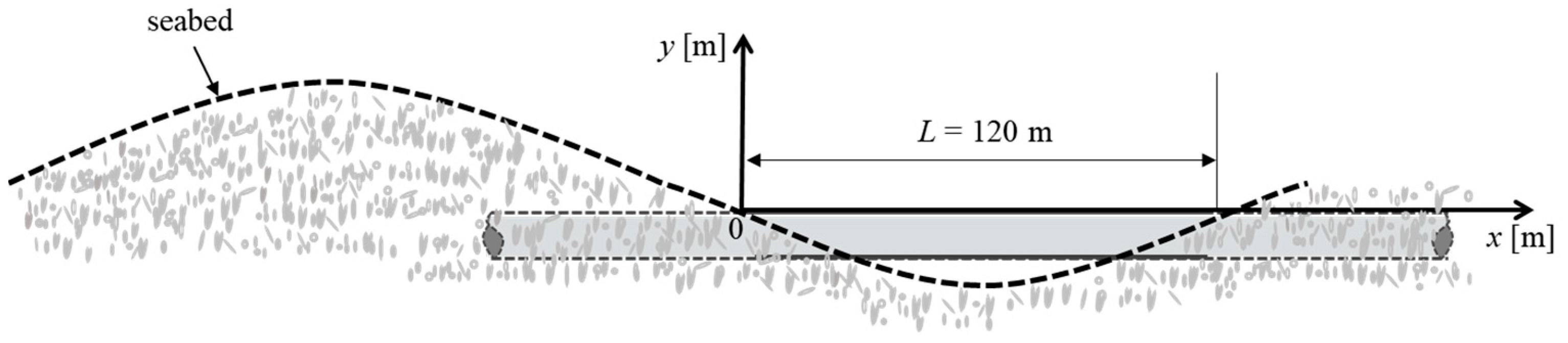
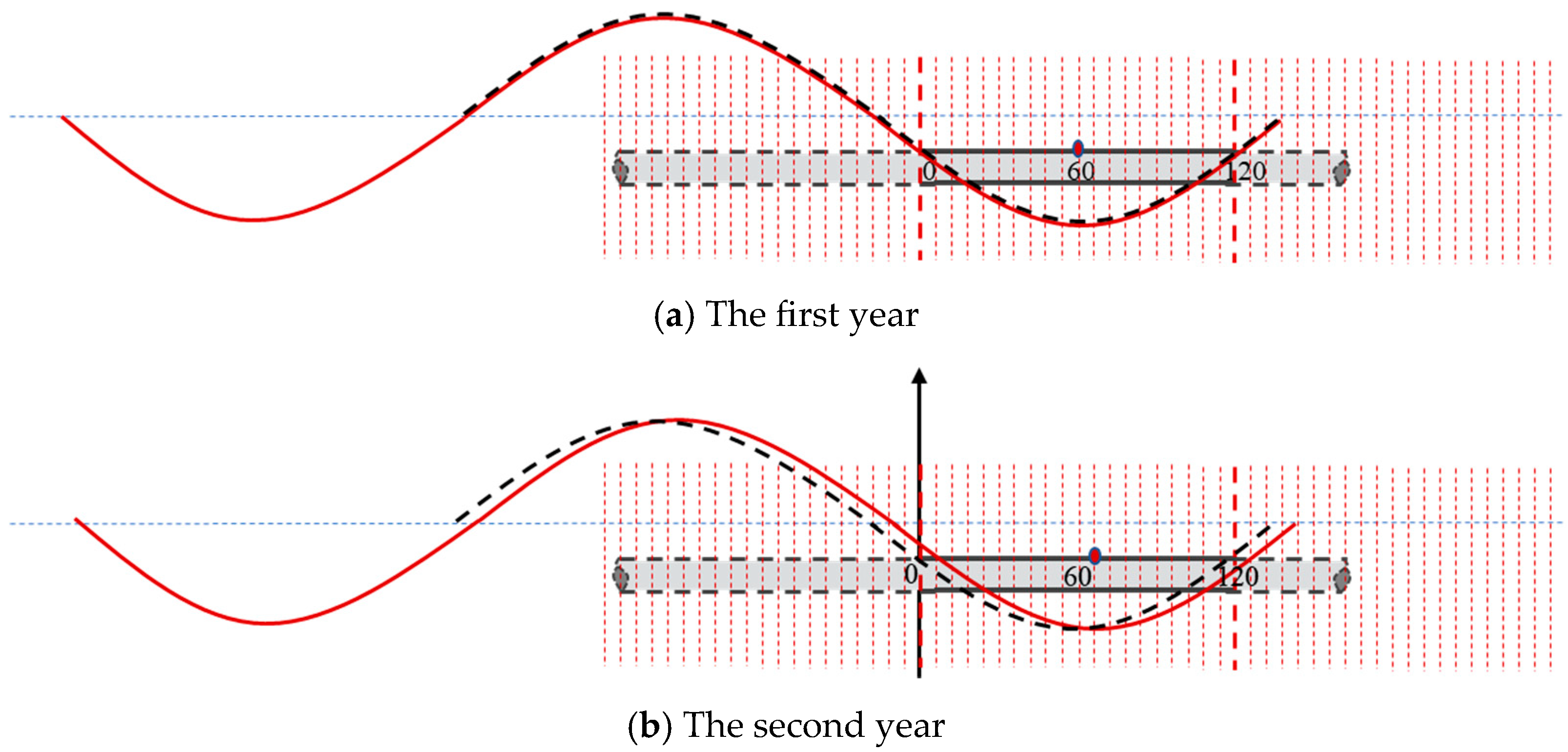
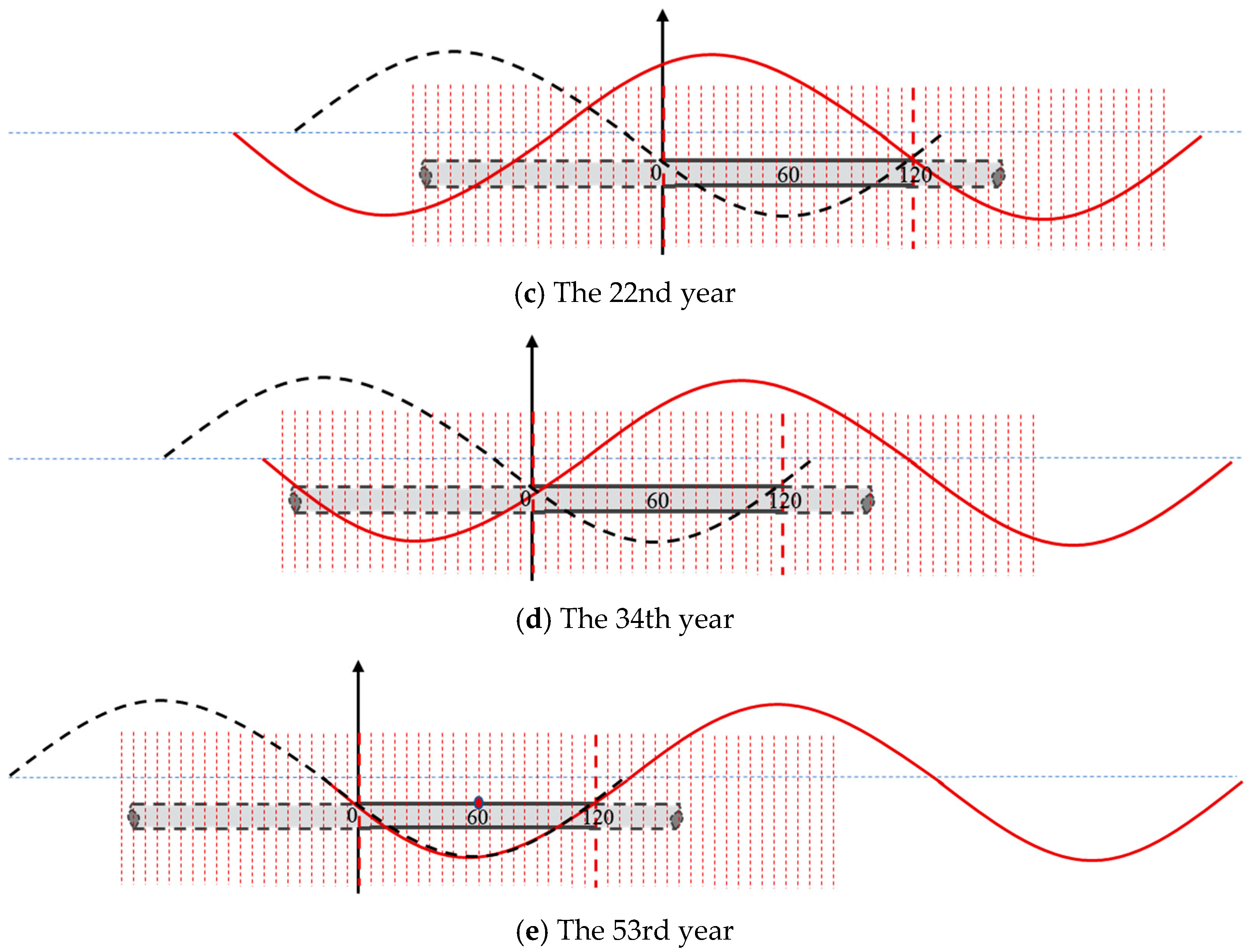
3.2. Fatigue Life Analysis of the Pipeline Under Changing Suspension Position Due to Sand Wave Migration

The seabed is not entirely flat. There are various seabed forms in many different areas (Knaapen [29]). Sand wave is a kind of seabed form, and its migration may lead to the formation and elimination of free spans. As the sand wave migrates, the suspension position will change correspondingly (Pu et al. [14]). This section aims to propose a method to compute fatigue damage and fatigue life of pipelines caused by sand wave migration. A sinusoidal sand wave migration is assumed.
Sand waves are widely distributed along the pipeline route areas. Engineering investigations show that their crest-to-crest distances vary from 200 m to 800 m, and the observed migration rates range from zero to tens of meters per year (Hulscher and Van Den Brink [30]; Bijker et al. [31]). In this section, the selected wavelength is 312 m, and the sand wave migration rate is 6 m per year. The parameters of the model are shown in Table 1. The model of this section is shown in Figure 9. The origin of the coordinates is located at the starting position of the span, and the span length is 120 m. The x-axis represents the direction of sand wave migration, and the y-axis represents the direction perpendicular to the seabed.
With the migration of sand waves, the buried and exposed parts of the pipeline change; that is, the suspension position changes and the span length of the studied pipeline remains unchanged. The migration process is shown in Figure 10, where the black dotted line indicates the initial position of the sand wave, and the red curve represents the moving sand wave. The red dot represents the suspension position. It can be seen from Figure 10 that the exposure and burial of the pipeline change periodically. The burial and exposure states of the pipeline due to sand wave migration are closely related to the fatigue damage of the pipeline.
At the initial moment, the mid-span position is at 60 m (Figure 10a). The chosen pipeline section is completely exposed, and the entire pipeline is considered when calculating the fatigue damage. One year later, the sand wave moves a certain distance, and the mid-span position moves a corresponding distance at 66 m (Figure 10b). During this period, part of the model is buried, and a new part of the pipeline will be exposed. Since we only focus on the chosen pipeline section, the new part is not considered when calculating the fatigue damage. In the 22nd year, the model is completely buried. At this moment, the buried model does not have fatigue damage (Figure 10c). As the sand wave continues to move, the model is exposed again, and only the fatigue damage of the exposed part of the model needs to be calculated (Figure 10d). After 53 years, all the chosen section is exposed again (Figure 10e). From Figure 10, the process is a complete cycle of 53 years. During this migration process, the pipeline is not vibrating all the time, so fatigue damage does not always occur.
For computing the fatigue life of the chosen pipeline section model during the migration process, the fatigue damage at each position of the pipeline is calculated once a year, and the fatigue analysis is carried out according to Section 2. In this way, the fatigue damages of the pipeline section at various points in different periods are calculated. The cumulative fatigue damage in 53 years of each point and its fatigue life are shown in Table 5. The fatigue life is about 1437 years. According to the traditional calculation method, the span position of the model remains unchanged. The pipeline is always in the suspended span state, and the pipeline vibrates continuously. According to the method proposed in Section 2, the fatigue life of the pipeline under a fixed span position is 177 years. Compared with the approach proposed in this study, the fatigue damage calculated by the traditional method is much larger. Accordingly, the fatigue life calculated by the proposed method is about eight times that of the traditional method. It is further verified that the traditional fatigue life analysis method is conservative.

4. Conclusions and Recommendations for Further Work

This study proposed probabilistic methods to study the pipeline’s fatigue life under the changes in span length and position due to the local scour and sand wave migration, respectively. For the uncertainty of the span length caused by the local scour, a mathematical transformation relation between the span length and fatigue life was first established. Then, the explicit solution of the fatigue life’s PDF was computed. The proposed method can quickly solve the fatigue life’s PDF under the various PDF of span length. Furthermore, the change process of span position due to sand wave migration is simulated. The fatigue damage of each point on the pipeline over a cycle is accumulated, and then the fatigue life of the pipeline is predicted. Conclusions were summarized as follows:
The suspension of a submarine pipeline is a dynamic process, and the span length varies with time. In this study, the PDF of the fatigue life of the pipeline was derived. The fatigue life of the pipeline based on the traditional method of the fixed free span was 177 years. The average fatigue life calculated by the different PDFs was 1837 years, 1766 years, and 1876 years, respectively, about 10 times that of a fixed 120 m long span.
The span position changes with time and space. This study accumulated the fatigue damage of the pipeline under different span positions over 53 years and the fatigue life of the pipeline under the condition that the span position changes were predicted. The fatigue life predicted in this condition was 1437 years, about eight times that of a fixed 120 m long span. The comparison results further verified that the moving span due to sand wave migration is beneficial in terms of the fatigue limit state of free spans.
The methodology can be universally adopted for the assessment of spans laying on sandy seabed. The simulation takes a couple of hours for a single case at a common laptop which is acceptable for span analysis. In engineering applications, the inputs, such as flow velocity, soil stiffness, damping ratio, pipeline properties, should be updated. The PDF of span length distribution should be replaced based on field scans of the as laid pipeline positions, e.g., with the multibeam echosounder (MBES). Moreover, the migration rate of sand waves should be captured based on numerical modeling or field scans within a couple of years.
The limitation is that the present work only considers the variation in free span length and position separately without considering the interaction between them. The geometry of sand waves might change during the sand wave migration, and local scour might happen together with the sand wave migration. Both these two phenomena will lead to the interaction of span length and position variations. In the future work, these two physical procedures need to be further investigated, after which the interaction between span length and position variations could be quantitatively assessed.

Author Contributions

Conceptualization and methodology, D.J., X.H. and G.T.; Software and Validation, D.Z. and H.Y.; formal analysis and investigation, D.J., X.H., D.Z., H.Y. and G.T.; writing—original draft preparation, X.H., H.Y. and G.T.; writing—review and editing, D.J. and G.T. All authors have read and agreed to the published version of the manuscript.

Funding

The author Guoqiang Tang would like to acknowledge the support from the National Nature Science Foundation of China through Grant 52371262.

Data Availability Statement

The data presented in this study are available from the corresponding author on request.

Conflicts of Interest

Daoyu Jiang, Xiaowei Huang and Deping Zhao were employed by EHV Transmission Company of China Southern Power Grid Co., Ltd. The remaining authors declare that the research was conducted in the absence of any commercial or financial relationships that could be construed as a potential conflict of interest.

Abbreviations

The following abbreviations are used in this manuscript:
VIVvortex-induced vibration
POFProbability of Failure
PDFProbability density function
COVCoefficient of Variation

References

  1. Kapuria, S.; Salpekar, V.Y.; Sengupta, S. Fatigue due to vortex-induced crossflow oscillations in free spanning pipelines supported on elastic soil bed. In Proceedings of the 9th International Offshore and Polar Engineering Conference, Brest, France, 30 May–4 June 1999. [Google Scholar]
  2. Fyrileiv, O.; Mørk, K. Structural response of pipeline free spans based on beam theory. In Proceedings of the 21st International Conference on Offshore Mechanics and Arctic Engineering, Oslo, Norway, 23–28 June 2002. [Google Scholar]
  3. Gamino, M. FSI Methodology for Analyzing VIV on Subsea Pipeline Free Spans with Practical Boundary Conditions. Ph.D. Thesis, Department of Mechanical Engineering Technology, University of Houston, Houston, TX, USA, 2013. [Google Scholar]
  4. Ulveseter, J.V.; Sævik, S.; Larsen, C.M. Vortex induced vibrations of pipelines with non-linear seabed contact properties. In Proceedings of the 35th International Conference on Ocean, Offshore and Arctic Engineering (OMAE2016-54424), Busan, South Korea, 19–24 June 2016. [Google Scholar]
  5. Yttervik, R.; Larsen, C.M.; Furnes, G.K. Fatigue from vortex-induced vibrations of free span pipelines using statistics of current speed and direction. In Proceedings of the ASME 2003 22nd International Conference on Offshore Mechanics and Arctic Engineering, Cancun, Mexico, 8–13 June 2003. [Google Scholar]
  6. Esplin, G.D.; Stappenbelt, B. Reducing conservatism in free spanning pipeline vortex-induced vibration fatigue analysis. Aust. J. Mech. Eng. 2011, 8, 11–20. [Google Scholar] [CrossRef]
  7. Gazis, N. A probabilistic approach for reliability assessment and fatigue analysis of subsea free spanning pipelines. In Proceedings of the Twenty-Second International Offshore and Polar Engineering Conference, Rhodes, Greece, 17–22 June 2012. [Google Scholar]
  8. Dong, J.; Chen, X.D.; Wang, B.; Guan, W.X.; Yang, T.X.; Fan, Z.C. The effect of soil on the structural response and fatigue life of free span for submarine pipeline. In Proceedings of the ASME Pressure Vessels and Piping Conference, Boston, MA, USA, 19–23 July 2015. [Google Scholar]
  9. Palmer, A. 10−6 and all that: What do failure probabilities mean? J. Pipeline Eng. 2013, 2, 109–111. [Google Scholar]
  10. Shabani, M.M.; Taheri, A.; Daghigh, M. Reliability assessment of free spanning subsea pipeline. Thin-Walled Struct. 2017, 120, 116–123. [Google Scholar] [CrossRef]
  11. Shabani, M.M.; Shabani, H.; Goudarzi, N.; Taravati, R. Probabilistic modelling of free spanning pipelines considering multiple failure modes. Eng. Fail. Anal. 2019, 106, 104169. [Google Scholar] [CrossRef]
  12. Li, X.H.; Zhang, Y.; Abbassi, R.; Khan, F.; Chen, G.M. Probabilistic fatigue failure assessment of free spanning subsea pipeline using dynamic Bayesian network. Ocean. Eng. 2021, 234, 109323. [Google Scholar] [CrossRef]
  13. Pinna, R.; Weatherald, A.; Grulich, J.; Ronalds, B.F. Field observations and modelling of the self-burial of a North West Shelf pipeline. In Proceedings of the 22nd International Conference on Offshore Mechanics and Arctic Engineering, Cancun, Mexico, 8–13 June 2003. [Google Scholar]
  14. Pu, J.J.; Xu, J.S.; Li, G.X. Self-burial and potential hazards of a submarine pipeline in the sand wave area in the South China Sea. J. Pipeline Syst. Eng. Pract. 2013, 4, 124–130. [Google Scholar] [CrossRef]
  15. Worden, K.; Farrar, C.R.; Manson, G.; Park, G. The fundamental axioms of structural health monitoring. Proc. R. Soc. A Math. Phys. Eng. Sci. 2007, 463, 1639–1664. [Google Scholar] [CrossRef]
  16. West, B.M.; Locke, W.R.; Andrews, T.C.; Scheinker, A.; Farrar, C.R. Applying Concepts of Complexity to Structural Health Monitoring. In Structural Health Monitoring, Photogrammetry & DIC; Springer: Cham, Switzerland, 2019; Volume 6, pp. 205–215. [Google Scholar]
  17. Ceravolo, R.; Civera, M.; Lenticchia, E.; Miraglia, G.; Surace, C. Detection and localization of multiple damages through entropy in information theory. Appl. Sci. 2021, 11, 5773. [Google Scholar] [CrossRef]
  18. Thorsen, M.J.; Sævik, S.; Larsen, C.M. Fatigue damage from time domain simulation of combined in-line and cross-flow vortex-induced vibrations. Mar. Struct. 2015, 41, 200–222. [Google Scholar] [CrossRef]
  19. Passano, E.; Larsen, C.M.; Lie, H.; Wu, J. VIVANA Theory Manual. User Manual; Norwegian University of Science and Technology: Trondheim, Norway, 2014. [Google Scholar]
  20. Sumer, B.M. Hydrodynamics Around Cylindrical Structures; World Scientific: Singapore, 2006. [Google Scholar]
  21. Dowling, N.E.; Calhoun, C.A.; Arcari, A. Mean stress effects in stress-life fatigue and the Walker equation. Fatigue. Fract. Eng. M. 2009, 32, 163–179. [Google Scholar] [CrossRef]
  22. Palmgren, A. Die lebensdauer von Kugellagern. Verfahrenstechnik Berl. 1924, 68, 339–341. [Google Scholar]
  23. Miner, M.A. Cumulative damage in fatigue. J. Appl. Mech. Sep. 1945, 12, A159–A164. [Google Scholar] [CrossRef]
  24. Leckie, S.H.F.; Draper, S.; White, D.J.; Cheng, L.; Fogliani, A. Lifelong embedment and spanning of a pipeline on a mobile seabed. Coast. Eng. 2015, 95, 130–146. [Google Scholar] [CrossRef]
  25. Lin, Y.K.M. Probabilistic Theory of Structural Dynamics; McGraw-Hill: New York, NY, USA, 1967. [Google Scholar]
  26. Cao, Q.Y.; Hu, S.L.J.; Li, H.J. Global maximum response of linear systems with uncertain damping to irregular excitation. J. Eng. Mech. 2020, 146, 04020043. [Google Scholar] [CrossRef]
  27. Det Norske Veritas. Recommended Practice DNV-RP-F105: Free Spanning Pipelines; DNV: Oslo, Norway, 2006. [Google Scholar]
  28. He, Z.F.; Wei, Y.; Liu, S.L. Analysis of safe span length and fatigue life of submarine pipelines. COE 2020, 34, 119–130. [Google Scholar] [CrossRef]
  29. Knaapen, M.A.F. Sandwave migration predictor based on shape information. J. Geophys. Res. Earth Surf. 2005, 110, 3. [Google Scholar] [CrossRef]
  30. Hulscher, S.J.M.H.; van den Brink, G.M. Comparison between predicted and observed sand waves and sand banks in the North Sea. J. Geophys. Res. Ocean. 2001, 106, 9327–9338. [Google Scholar] [CrossRef]
  31. Bijker, R.; Wilkens, J.; Hulscher, S. Sandwaves: Where and why. In Proceedings of the Eighth International Offshore and Polar Engineering Conference, Montreal, QC, Canada, 24 May 1998. [Google Scholar]
Figure 1. The sketch of the formation of free span due to local scour.
Jmse 13 00763 g001
Figure 2. Seabed–pipe interaction model.
Jmse 13 00763 g002
Figure 3. Comparison of response amplitude ratio distribution.
Jmse 13 00763 g003
Figure 4. Comparison of the stress amplitude distribution.
Jmse 13 00763 g004
Figure 5. Fatigue damage in one year.
Jmse 13 00763 g005
Figure 6. PDF of P(T) with P1(L).
Jmse 13 00763 g006
Figure 7. PDF of P(T) with P2(L).
Jmse 13 00763 g007
Figure 8. PDF of P(T) with P3(L).
Jmse 13 00763 g008
Figure 9. Pipeline model.
Jmse 13 00763 g009
Figure 10. The change process of pipeline suspension position.
Jmse 13 00763 g010aJmse 13 00763 g010b
Table 1. Model parameters.
ParameterSymbolValue
Outside diameter/(m)D0.55
Wall thickness/(m)d0.02
Pipeline mass for unit length/(kg/m)mp315
Young’s modulus/(Pa)E2.08 × 1011
Bending stiffness of pipeline/(N/m)EI2.9 × 108
Span length/(m)L120
Shoulder length/(m)LS130
Current velocity/(m/s)U0.7
Water density/(kg/m3)ρ1025
Vertical soil stiffness/(N/m)kb40,000
Table 2. The data of span length and fatigue life.
Span length (m)120117……6360……1512……0
Fatigue life (year)177315……18932494…………
Table 3. The average fatigue life calculated by the different PDFs.
Probability Density CurveTruncated GaussianRayleighUniform
E(T)/(year)183717661876
Table 4. The average fatigue life calculated by the probability density curve.
COVCOVLCOVT
Probability Density Curve
Truncated Gaussian distribution0.47232.9459
Rayleigh distribution0.46492.7337
Uniform distribution0.57742.8033
Table 5. The calculation results of fatigue damage at each point under the varying suspension position.
Position (m)
In Year024487296120
11.24 × 10−101.58 × 10−53.70 × 10−34.13 × 10−33.20 × 10−57.28 × 10⁻¹¹
2 1.33 × 10−72.14 × 10−35.29 × 10−33.10 × 10−46.81 × 10⁻¹¹
3 1.13 × 10−108.95 × 10−45.63 × 10−31.13 × 10−31.33 × 10−10
4 6.57 × 10−112.20 × 10−45.16 × 10−32.58 × 10−31.33 × 10−7
5 1.24 × 10−101.58 × 10−53.70 × 10−34.13 × 10−33.20 × 10−5
6 1.33 × 10−72.14 × 10−35.29 × 10−33.10 × 10−4
7 1.13 × 10−108.95 × 10−45.63 × 10−31.13 × 10⁻³
8 6.57 × 10−112.20 × 10−45.16 × 10−32.58 × 10⁻³
9 1.24 × 10−101.58 × 10−53.70 × 10−34.13 × 10⁻³
10 1.33 × 10−72.14 × 10−35.29 × 10⁻³
11 1.13 × 10−108.95 × 10−45.63 × 10−3
12 6.57 × 10−112.20 × 10−45.16 × 10−3
13 1.24 × 10−101.58 × 10−53.70 × 10−3
14 1.33 × 10−72.14 × 10−3
15 1.13 × 10−108.95 × 10⁻⁴
16 6.57 × 10−112.20 × 10⁻⁴
17 1.24 × 10−101.58 × 10⁻⁵
18 1.33 × 10⁻⁷
19 1.13 × 10⁻¹⁰
20 6.57 × 10⁻¹¹
21 1.24 × 10⁻¹⁰
……
337.28 × 10⁻¹¹
346.81 × 10⁻¹¹
351.33 × 10⁻¹⁰
361.33 × 10⁻⁷
373.20 × 10−57.28 × 10−11
383.10 × 10−46.81 × 10−11
391.13 × 10−31.33 × 10−10
402.58 × 10−31.33 × 10−7
414.13 × 10−33.20 × 10−57.28 × 10⁻¹¹
425.29 × 10−33.10 × 10−46.81 × 10⁻¹¹
435.63 × 10−31.13 × 10−31.33 × 10⁻¹⁰
445.16 × 10−32.58 × 10−31.33 × 10⁻⁷
453.70 × 10−34.13 × 10−33.20 × 10−57.28 × 10−11
462.14 × 10−35.29 × 10−33.10 × 10−46.81 × 10−11
478.95 × 10−45.63 × 10−31.13 × 10−31.33 × 10−10
482.20 × 10−45.16 × 10−32.58 × 10−31.33 × 10−7
491.58 × 10−53.70 × 10−34.13 × 10−33.20 × 10−57.28 × 10⁻¹¹
501.33 × 10−72.14 × 10−35.29 × 10−33.10 × 10−46.81 × 10⁻¹¹
511.13 × 10−108.95 × 10−45.63 × 10−31.13 × 10−31.33 × 10−10
526.57 × 10−112.20 × 10−45.16 × 10−32.58 × 10−31.33 × 10−7
531.24 × 10−101.58 × 10−53.70 × 10−34.13 × 10−33.20 × 10−57.28 × 10⁻¹¹
Sum in 53 years3.12 × 10−23.12 × 10−23.49 × 10−23.54 × 10−23.13 × 10−23.12 × 10⁻²
Fatingue life (year)169716961518149916961697
Disclaimer/Publisher’s Note: The statements, opinions and data contained in all publications are solely those of the individual author(s) and contributor(s) and not of MDPI and/or the editor(s). MDPI and/or the editor(s) disclaim responsibility for any injury to people or property resulting from any ideas, methods, instructions or products referred to in the content.

