Interfacial Failure in Flexible Pipe End Fittings: DIC and Cohesive Zone Modeling for Defect Analysis

Abstract

Flexible pipe end fittings (EFs) transfer axial loads by embedding tensile armor within epoxy matrices. The integrity of bonding between the armor and resin profoundly influences the EF load-bearing capacity. This study investigated the debonding failure mechanism at the epoxy-resin–tensile-armor interface in flexible pipe end fittings through integrated experimental and numerical approaches. Combining tensile tests with digital image correlation (DIC) and cohesive zone modeling (CZM), the research quantified the impacts of interfacial defects and adhesive properties on structural integrity. Specimens with varying bond lengths (40–60 mm) and defect diameters (0–4 mm) revealed that defects significantly reduced load-bearing capacity, with larger defects exacerbating strain localization and accelerating failure. A dimensionless parameter, the defect-size-to-bond-length ratio ($\lambda =D/2L$), was proposed to unify defect impact analysis, demonstrating its nonlinear relationship with failure load reduction. High-toughness adhesives, such as Sikaforce^® 7752, mitigated defect sensitivity by redistributing stress concentrations, outperforming brittle alternatives like Araldite^® AV138. DIC captured real-time strain evolution and crack propagation, validating strain concentrations up to 3.2 at defect edges, while CZM simulations achieved high accuracy (errors: 3.0–7.2%) in predicting failure loads. Critical thresholds for λ (λ < 0.025 for negligible impact; λ > 0.05 requiring defect control or high-toughness adhesives) were established, providing actionable guidelines for manufacturing optimization and adhesive selection. By bridging experimental dynamics with predictive modeling, this work advances the design of robust deepwater energy infrastructure through defect management and material innovation, offering practical strategies to enhance structural reliability in critical applications.

1. Introduction

The expansion of oil and gas exploration into deepwater regions in recent years has significantly increased the demand for flexible pipes [1]. Each unbonded flexible pipe is meticulously engineered to withstand specific loads, including tension, internal pressure, external pressure, and torsion [2]. 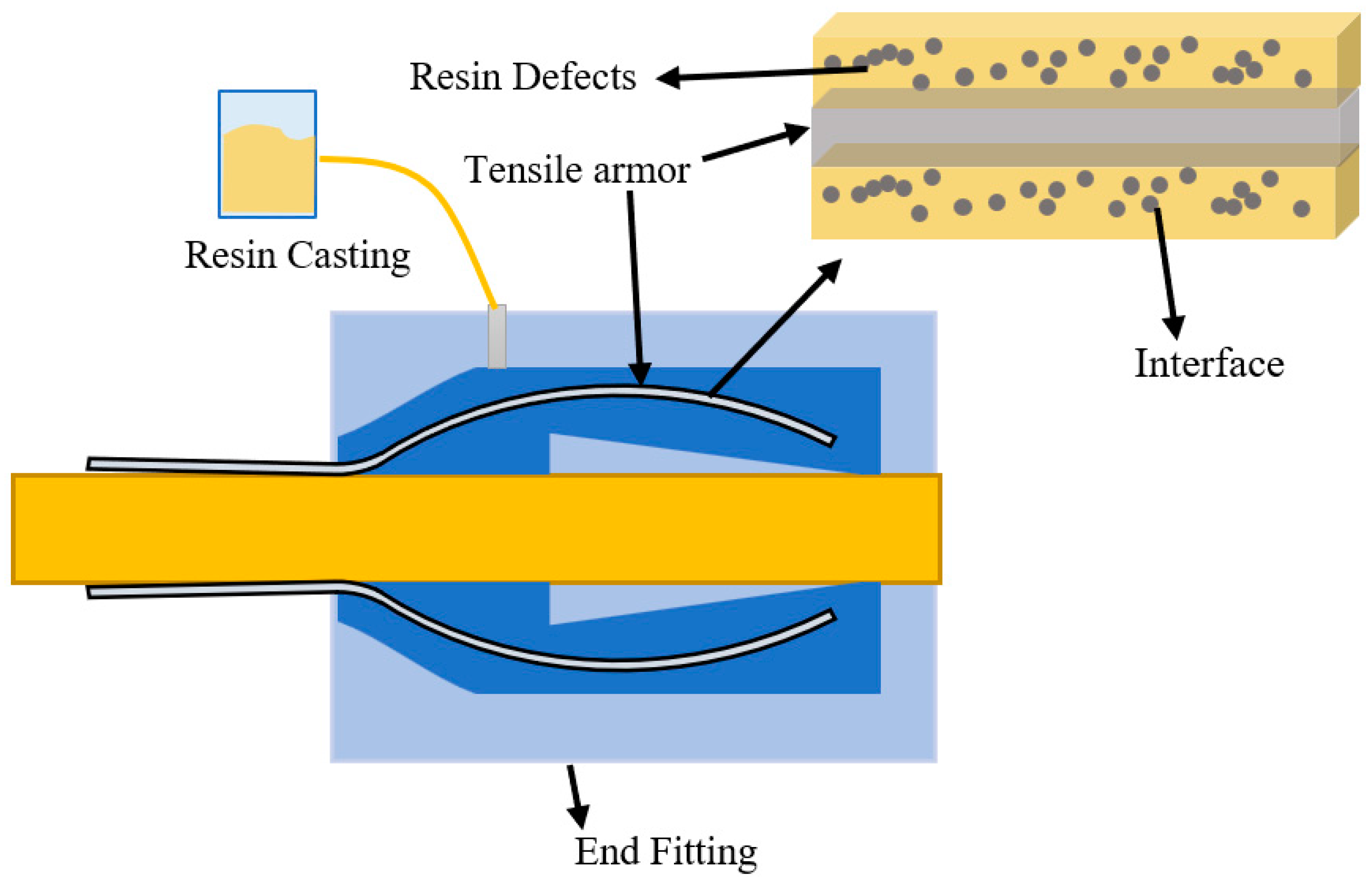A typical flexible pipe comprises several layers, such as an internal carcass layer, a pressure barrier layer, pressure armor layers, tensile armor layers, and an anti-abrasion layer, all encased within an outer sheath [3]. End fittings are specially designed to connect these layers and facilitate the necessary connections with the customer’s production facility. A typical end fitting structure is shown in Figure 1.

Researchers have extensively investigated the mechanical properties of the tensile armor within flexible pipes, particularly focusing on the impact of end restraints. End fitting regions have received significant attention because they represent the weakest points in the entire pipe system [4]. Studies have shown that these constraints lead to stress concentrations in the steel wires near the end fittings [5]. Numerical methods are frequently employed to predict stress concentrations within tensile armor, with the wire geometry being a primary factor in stress distribution [6]. Moreover, residual stresses induced by wire folding during end-fitting operations have been identified as significant contributors to end fitting and wire failure, ultimately reducing the fatigue life of the pipes [7]. Mid-scale model tests have confirmed the adverse effects of end-fitting constraints on fatigue performance, particularly through the examination of S-N curves [8]. Additionally, fiber-optic measurements have been used to highlight stress concentration effects by measuring steel wire strain [9].

Accurately characterizing the interaction between the steel wire and the resin is crucial because the adhesive interaction has a substantial impact on the performance of flexible pipe end fitting [10]. Numerical methods are commonly used to simulate the interfacial failure behavior of bonded structures similar to end fittings. Though it is essential to consider the adhesive effect as a kind of friction when assessing the anchoring capacity of the fitting, correctly characterizing the fracture failure between the steel wire and the resin presents a significant challenge [11]. Fracture mechanics methods that are commonly used to describe the fracture failure of the adhesive interface include the Cohesive Zone Method [12], XFEM [13], and VCCT [14]. The progressive failure behavior of flexible pipe end fittings was investigated through cohesive zone modeling, demonstrating that interfacial bonding constitutes a critical controlling factor for the connection performance, with mechanical response characteristics showing significant correlation with adhesive layer failure mechanisms [15]. Although there have been few reports in the literature, some scholars have employed experimental methods to investigate the interfacial failure of end fittings. Thermal imaging has been demonstrated to be an effective technique for instantly monitoring interfacial damage caused by cyclic stress [16]. Conventional techniques meet difficulties in accurately evaluating the detailed deformation of bonded structures in actual time while digital image correlation (DIC) is capable of accurately recording the complete deformation of a structure and bond damage condition. For example, the DIC approach allows us to evaluate the behavior of single lap joints when they fail and to record, in real time, the procedures and mechanisms of fatigue failure in joints made of carbon and aluminum. Furthermore, the DIC approach was used in a study to explore the fatigue failure process and failure mechanism of carbon–aluminum bonding [17].

The complex structure of the tensile armor can result in insufficient flow within the end-fitting cavity during casting, leading to defects of varying sizes near the steel wires [18], as depicted in Figure 2. One of the most critical factors affecting the performance of end-fitting connections is the presence of cavity defects formed during the casting process. However, the literature on processing defects in flexible pipe end fittings is limited due to the large structural scale and the non-periodic helical arrangement of the internal steel wire. Finite element simulations quantifying void defect effects have revealed that epoxy adhesives show 18% lower stress concentration than polyurethane counterparts under equivalent shear loading conditions [19]. The study cited utilized numerical methods to investigate the effects of voids in the adhesive layer both on the bond strength in lap joints and on the stress concentration in the adhesive layer due to the existence of voids. The results showed that the sizes of the voids had the most significant effect on the reduction in bond strength [20]. Interface defects, including voids, microcracks, and delamination, are widely recognized as critical factors influencing the structural integrity and failure of adhesive joints and composite materials. These defects often serve as stress concentrators, initiating localized material degradation and ultimately leading to catastrophic failure under mechanical loading conditions [21]. For instance, the presence of voids can substantially diminish the load-bearing capacity of adhesive joints, while delamination tends to propagate rapidly under cyclic loading or shear stress [22,23]. In the specific context of flexible pipe end fit tings, these failure mechanisms are particularly pronounced due to the complex stress states and harsh environmental conditions to which these systems are subjected. A comprehensive understanding of the initiation and evolution of such defects is, therefore, imperative for the development of more robust and reliable adhesive bonding systems.

The helical geometry of flexible pipe end fittings induces multi-axial stress states under operational loads, complicating direct experimental replication. While existing research has extensively explored stress concentrations and numerical simulations (e.g., cohesive zone modeling and XFEM) for interfacial failure analysis, critical gaps persist in quantifying the impact of manufacturing defects—particularly cavity voids formed during casting due to the non-periodic helical arrangement of tensile armor. To address this, simplified uniaxial specimens were designed to isolate defect-driven failure mechanisms (e.g., strain localization and crack propagation) by preserving two critical parameters: the defect-size-to-bond-length ratio $(\lambda =D/2L)$ and material toughness ($\Gamma =G_{IC}/{\sigma }_f$). This approach aligns with composite joint methodologies, where controlled experiments on reduced-scale geometries yield insights transferable to complex systems. By integrating tensile tests with full-field DIC strain mapping and CZM simulations, this study systematically linked defect geometry and material properties to interfacial debonding. The proposed λ–Γ framework establishes predictive tools for defect tolerance optimization, validated by numerical results matching experimental strain fields (errors: 3.0–7.2%). These findings bridge idealized models with real-world helical behavior, offering actionable guidelines for adhesive selection and defect control in deepwater pipeline reliability. This study investigated the interaction between defect geometry, adhesive properties, and structural degradation, a previously underexplored aspect, and provided a quantitative framework to improve the integrity of flexible pipe end fittings.

2. Specimen Preparation

This research examined the effects of different defect sizes by fabricating tensile specimens with different defect sizes, as illustrated in Figure 3. The bonding length (L) of the wire was available in three specific lengths: 40 mm, 50 mm, and 60 mm. Additionally, the diameter D of the semicircular defect varied, with dimensions of 0 mm (indicating no defect), 2 mm, and 4 mm. The specimens were constructed using SAE 1070 high-strength tensile armor (Mingjie steel, Dongguan, China) and bonded using Araldite^® 2015 adhesive (Huntsman Advanced Materials (Shanghai) Co., Ltd., Shanghai, China). The selection of SAE 1070 steel ensured that the specimen remained within the elastic range during the tensile test, thereby mitigating any potential influences from yield-related effects on the experimental outcomes. Araldite^® 2015 was chosen for its widespread application in cohesive zone modeling (CZM), which supported the research on its cohesive parameters, microstructure, and fracture characteristics. The fundamental material properties were sourced from the supplier and are detailed in

Table 1. Properties of specimen material.

Material	Araldite® 2015	SAE 1070
Young’s modulus, E [GPa]	1.85	205
$\mathrm{Poisson}’\mathrm{s}\mathrm{ratio},\nu$	0.33	0.3
$\mathrm{Tensile}\mathrm{yield}\mathrm{stress},{\sigma }_y$ [MPa]	12.63	1268
$\mathrm{Tensile}\mathrm{strength},{\sigma }_s$ [MPa]	21.63	1422

.

The fabrication of bonded specimens involves a meticulously controlled multi-step process designed to optimize the strength and durability of the bond. Initially, the specimen surfaces undergo a thorough cleaning regimen, employing a solution of isopropyl alcohol and water to remove any oils and contaminants. Subsequently, the surfaces are polished to enhance adhesive bonding. In this study, the adhesive preparation followed strict adherence to the manufacturer’s guidelines (the adhesive was cured at 25 °C for 24 h). A plastic semi-cylindrical mold coated with a release agent was pre-embedded at the bonding interface. After curing, the mold was removed to create predefined defects, ensuring dimensional accuracy.

3. DIC Experiment

Digital image correlation (DIC) is a non-contact, full-field optical technique used to measure the strain, displacement, and deformation of an object. The methodology comprises three crucial stages:

(1)

Speckle Application: In the initial preparation phase, speckles are applied to the surface of the specimen. These speckles form a high-contrast, random, isotropic, and stable pattern essential for accurate strain measurements. Techniques such as gun spraying, photolithography, and spin coating are employed to achieve speckle patterns that fulfill these stringent criteria.

(2)

Image Acquisition: During the testing phase, images are captured at various stages of loading. It is crucial to position the camera sensor optimally concerning the specimen to minimize geometric distortions and ensure high-quality images. This positioning is vital in high-resolution systems to avoid any impact on the correlation and matching accuracy of the images.

(3)

Image Analysis: The final step involves analyzing the captured images using a correlation algorithm. DIC utilizes a subset of pixel values to track the movement of points across the original and deformed images. Each subset features a broad greyscale distribution, aiding in the precise localization of the subset in the deformed image. Unique features within each deformed subset facilitate its distinction from other subsets. Figure 4 illustrates the displacement mapping in DIC, demonstrating the relationship between a reference subset and a deformed subset.

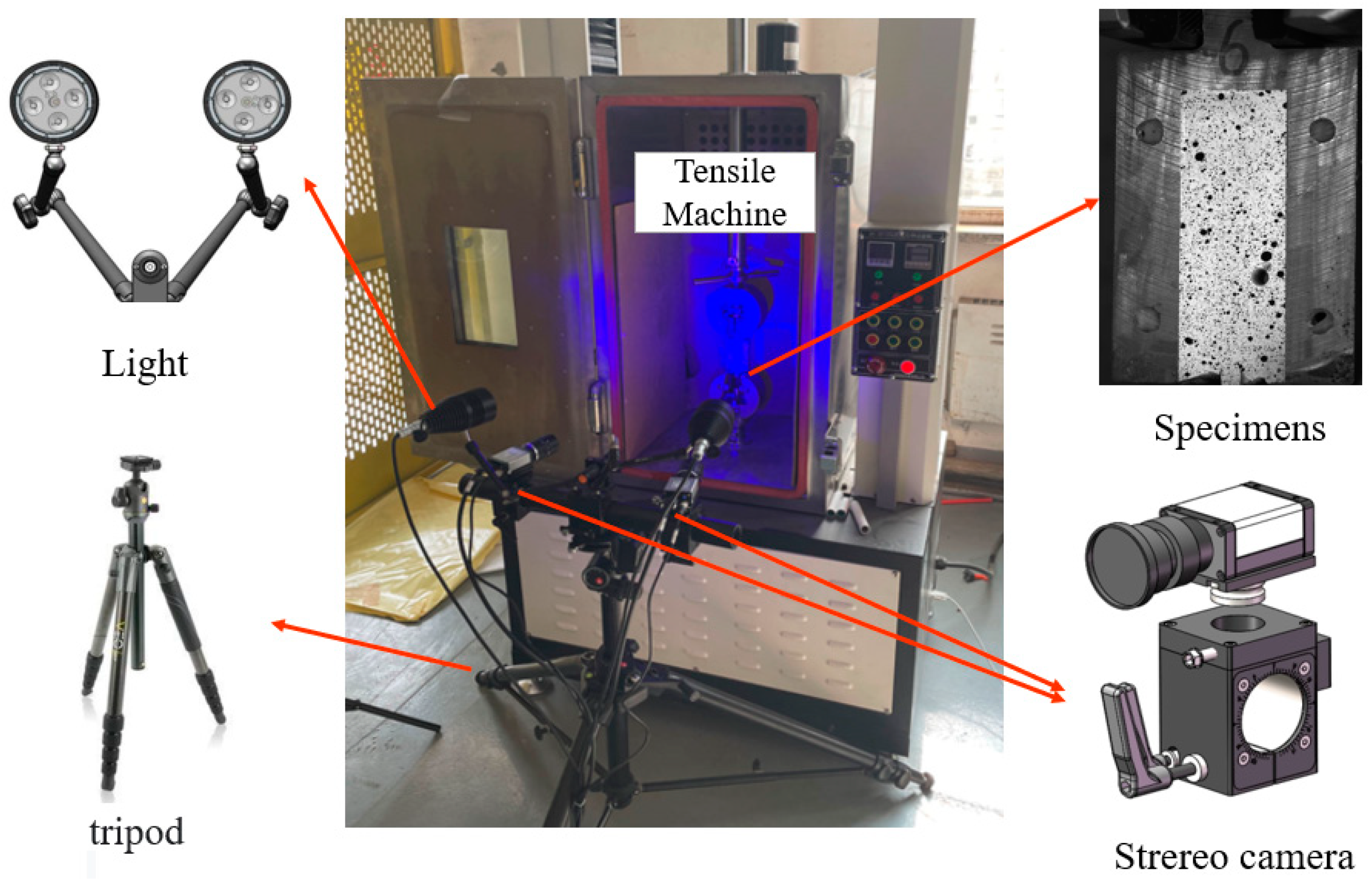
The experiments were conducted using the advanced revealer DIC-3D technique, utilizing two GigE CCD cameras (PMLAB, Hefei, China), each boasting a resolution of 4096 × 3000 pixels. These cameras were equipped with Ricoh 50 mm lenses and strategically positioned at a distance of 300 mm from the specimen. The cameras were securely fixed on a tripod. The experiment setup commenced with the precise alignment of the imaging system. The cameras were arranged perpendicular to the specimen at approximately 50 cm and adjusted to the correct height to optimize the field of view. Each camera was configured to cover an overlapping field of view measuring 20 cm × 20 cm, which was critical for the accurate functioning of the associated image processing algorithms. Calibration of the cameras was carried out at an angle of approximately 45° using a standard checkerboard pattern with a 9 × 12-point grid. This calibration process involved repositioning the calibration target multiple times within the measurement volume to capture a comprehensive set of images. These images were then analyzed to extract both internal and external calibration parameters, ensuring the precision of subsequent measurements.

To achieve synchronization between the initiation of the tensile testing and the image acquisition, a trigger signal was employed. The cameras captured images at a frequency of 5 Hz throughout the experiment, allowing for detailed analysis of the specimen behavior under load.

The mechanical testing of the specimens was performed using a displacement-controlled testing machine, which applied a constant loading rate of 2 mm/min. This procedure was continued until the failure of the specimens, with all displacement and load data being automatically recorded by the system. The setup of the experiment, along with the positioning of the equipment, is illustrated in Figure 5.

4. Experiment Results

4.1. Failure Load

The load-displacement curve is a fundamental graphical representation of the relationship between applied mechanical load and the resulting displacement in a joint. The peak load, representing the maximum force a specimen can withstand before failure, serves as a key indicator of bond strength. As a critical parameter, it provides a direct measure of the effectiveness and durability of adhesive bonds, making it a standard criterion for evaluating joint performance across various applications.

Figure 6 presents the load-displacement curves of the tested specimens, all of which exhibited brittle failure characterized by rapid crack propagation and a subsequent decline in load-bearing capacity. As shown in Figure 6a, the failure load increased with bond length, with the L = 60 mm specimen exhibiting 34% and 13% higher failure loads than those with L = 50 mm and L = 40 mm, respectively. Figure 6b–d further illustrate the effect of defect size and bond length, revealing that for specimens with L = 40 mm, L = 50 mm, and L = 60 mm, the presence of a D = 4 mm defect led to failure load reductions of 9.5%, 8.8%, and 8.0%, respectively, compared to non-defective specimens. These findings demonstrate that defects reduce load-bearing capacity, with larger defect areas causing greater reductions. The extent of this reduction correlates with the ratio of defect length to bond length, emphasizing the importance of defect management in maintaining joint integrity and optimizing performance.

Figure 6e presents the mean failure loads and standard deviations (SD, N = 3) for nine specimen groups, combining three bond lengths (L40, L50, L60) and three defect sizes (D0, D2, D4). The failure load increased with bond length: defect-free specimens (D0) achieved 5.66 ± 0.09 kN (L40), 6.68 ± 0.11 kN (L50), and 7.59 ± 0.15 kN (L60), demonstrating a 34% improvement from L40 to L60. Conversely, larger defects reduced load-bearing capacity—for example, L40-D4 specimens (5.12 ± 0.12 kN) showed a 9.5% decrease compared to L40-D0. Notably, an increased bond length partially mitigated defect effects: L60-D4 specimens (6.98 ± 0.21 kN) retained 82% of the defect-free L60 capacity, outperforming L40-D4 by 36%. Tight standard deviations (±0.09–0.21 kN) confirmed data reproducibility, supporting the reliability of the observed trends.

4.2. Failure Mode

Theoretically, the bond interface between tensile armor and epoxy in flexible pipe end fitting can exhibit four primary failure modes: at the steel-plate–bond layer interface, colloid bond failure, yielding of the steel plate, and hybrid failure, which involves damage at the steel plate interface. In our experiments, due to the short bonding length of the tensile armor, that did not reach its yield point. It was observed that either increasing the bonding length or altering the wire’s geometry could induce yielding, which may have manifested as a distinct plateau in the load-displacement curve. This phenomenon indicated a shift in the failure mechanism, underscoring the wire’s significant contribution to the overall failure process. Understanding these diverse failure modes is essential for the design and analysis of bonded structures as it enables more accurate predictions of their behavior under load. Such knowledge can also guide strategies to enhance their structural strength and durability.

Under displacement loading, cracking was observed at the steel plate and bond interface, accompanied by a gradual debonding process. Concurrently, the distinct fracture sound emitted by the adhesive suggested that the Araldite^® 2015 adhesive exhibited brittle characteristics. Notably, some specimens exhibited processing failures, such as adhesive residue on the wire, likely due to imperfect prefabrication techniques.

The relative strengths of the interfacial and adhesive components play a determinant role in determining the failure mode of the specimen. In specimens devoid of prefabricated defects and possessing strong adhesive strength, the primary failure mode observed was adhesive interface debonding, as depicted in Figure 7. Conversely, specimens with prefabricated defects displayed both macroscopic and internal microscopic defects, which compromised the bond strength. This condition resulted in the wire pulling out while localized damage occurred within the adhesive. The experimental outcomes suggested that the failure of steel-wire-reinforced epoxy-bonded flexible pipe end fittings was predominantly related to the interface, although the adhesive’s properties also influenced the failure mode. The presence of processing defects further predisposed the adhesive to damage, emphasizing the need for meticulous control over fabrication processes to mitigate such vulnerabilities.

4.3. DIC Results

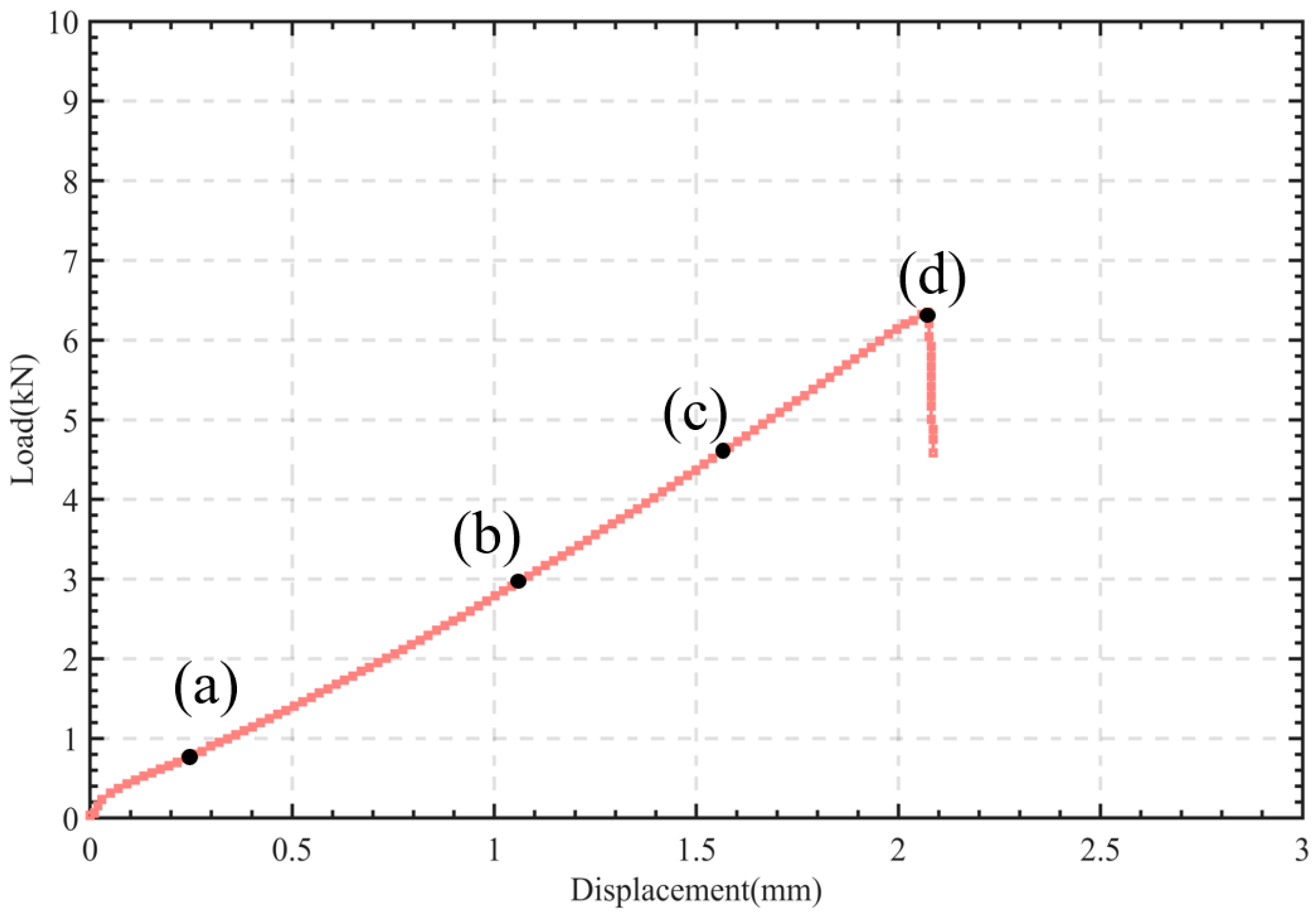
Figure 8 illustrates the load-displacement curve for the SP4 (L50-D0) specimen, highlighting four critical points that correspond to the 10%, 50%, 75%, and 100% failure displacement stages. An examination of the strain field results at these designated displacements allows for a detailed investigation into the history of the damage of the bonded structure. This analysis is instrumental in elucidating the progressive deterioration and the structural response at various phases of loading, which is crucial for comprehending the behavior of the bonded interface when subjected to tensile stress.

Figure 9 delineates the evolution of the strain field throughout the destruction of the bonded structure, focusing on the interface between the wire and the epoxy. This analysis is essential for comprehending the response and damage mechanisms of the structure under tensile loading. The strain field mapping reveals areas of high stress, pathways for crack extension, and points of bond separation. Such insights are vital for optimizing bond design and material selection to enhance the durability and reliability of the structure under stress.

As depicted in Figure 9a, the observed strain was minimal due to the adhesive’s elastic modulus being significantly lower than that of the steel wire, resulting in greater strain within the colloidal area compared to the wire. Figure 9b shows that at 25% failure displacement, distinct strain patterns became evident in the steel wire, bonding interface, and colloidal phase, as seen from the strain contour plot. With further loading, as illustrated in Figure 9c, the strain distribution remained largely consistent; the steel wire exhibited the lowest strain, and the bonding interface near the wire showed higher strain than the wire itself but lower than the colloidal area. As loading continued, the bonding components began to fail, and the interface started to crack, as indicated in Figure 9d. The cracks extended along the bond interface and load transfer direction, resulting in a gradual loss of shear load transfer capacity. Simultaneously, significant strain redistribution occurred in the interface zone, leading to a markedly lower strain in the wire and adhesive compared to the interface crack extension zone.

4.4. Interfacial Strain Evolution

To further explore the failure behavior, digital image correlation (DIC) was employed to capture the evolution of strain at the bonded interface. Eleven points (P1–P11) were selected along the interface, with P1 located at the starting point (y = 0) and P11 at the end point (y = 50 mm), 5 mm apart. The selection scheme is depicted in Figure 10, which shows the interface strain point selection map.

Figure 11 illustrates the evolution of strain at selected points over the loading history. The data reveal two stages of progression. Initially, during the loading phase, strain at each point increased with loading, exhibiting a minimal overall increase. Typically, the strain decreased from P1 to P11 due to load depletion in interfacial shear.

The subsequent stage was characterized by failure, where the strain time–history curve exhibits an inflection point, indicating a significant increase in strain. This sharp rise in strain signals interfacial bond rupture. Strain initially increases at P1, followed by an inflection point at P2, and progresses gradually to P11. This pattern indicates that crack propagation occurred from the outer edge towards the center.

4.5. Local Strain Concentration

In the exploration of how defects influence failure mechanisms, this study employed digital image correlation (DIC) techniques to perform full-field strain measurements. Special emphasis was placed on the phenomenon of localized strain concentrations around defective regions, which remain undetectable using conventional measurement method.

Figure 12 displays the strain evolution at six points in proximity to a 2 mm defect within the specimen (SP5 (L50-D2)). Points A and B, located at −5 mm and −2 mm, respectively, and points C and D at +2 mm and +5 mm, are positioned away from the defect. Conversely, points E and F are situated at the defect’s edge. The analysis of the data presented in Figure 12 reveals significantly higher strain levels at points E and F, located at the defect’s edge, compared to other points. This observation validates the DIC technique’s efficacy in detecting strain concentrations as the specimen approached failure. The strain at each point escalated as the tensile load increased, and the strain concentration became more pronounced as the tensile load increased.

In this study, the level of strain concentration was quantified using a strain concentration factor (SCF). The SCF was determined by dividing the maximum strain observed at the defect site by the average strain measured in an area not affected by the defect. For example, in the case of Figure 12, SCF = ${\epsilon }_E∕{\epsilon }_A$.

Figure 13 illustrates the variation of strain concentration factor (SCF) over time for specimens with defects of different sizes (i.e., 2 mm and 4 mm). As the loading time progressed, the SCF initially displayed a linear increase corresponding to the increasing tensile load. In the early stages of loading, the SCF exhibited a linear increase in response to the increasing tensile load. However, as the specimen approached the failure stage, the SCF escalated at a faster rate.

By comparison, it is evident that the SCF trends for smaller and larger defects were similar, yet the SCF values were consistently higher for smaller defects. This can be attributed to the more abrupt changes in the geometrical configuration associated with smaller defects, which consequently resulted in a larger SCF. The disparity in SCF values between the two defect sizes emphasizes the influence of defect geometry on the response of the structure to applied loads.

5. Numerical Model

5.1. Cohesive Zone Model (CZM)

In this research, bonded components were modelled using three-dimensional FEA in ABAQUS 2022, ensuring consistency with the dimensions of the experimental setup. The finite element model was instrumental in predicting failure loads and elucidating the effects of defects on failure mechanisms. When examining defects of varying sizes, the 3D model provided enhanced accuracy in predicting failure loads and detailing stress distributions, as is shown in Figure 14.

Cohesive zone models (CZMs) are employed to predict failure loads and capture the interaction between the wire and the adhesive through cohesive behavior. Within the CZM framework, fracture formation is treated as a progressive event occurring at an extended crack tip, or cohesive zone, subjected to cohesive traction forces. The traction–separation law integral to CZMs delineates the relationship between cohesive traction and the corresponding displacement separation at the crack surface. The stress distribution at any given location can be measured by the range of openings, which is essential for the accurate prediction of delamination in bonded structures. The law demonstrates a direct relationship between the cohesive traction vector and the displacement separation vector acting on the fracture surface. For interfaces involving brittle adhesives, the bilinear model is often sufficient and computationally efficient to implement [24].

Figure 15 depicts the traction–separation law for a singular fracture mode. In scenarios where a single fracture mode is predominant, crack initiation occurs at ${\sigma }_c$. As the bonding system is subjected to loading, the relative displacement of the contact surfaces generates contact stress within the cohesive zone. The constant K represents the proportionality between the contact stress and the separation at the interface prior to the initiation of damage. ${\delta }_c$ denotes the critical separation at which damage occurs. Subsequently, the damage progresses, leading to a reduction in interface stiffness. Upon reaching the maximum displacement ${\delta }_{sep}$, the contact surfaces become completely separated. The extent of damage is quantified using the damage parameter D.

5.2. Numerical Results

Concurrently, a finite element model was constructed to match the scale of the experimental setup, and

Table 2. Comparison between finite element method and experimental results.

No.	Specimen Name	${\mathit{P}}_{\mathit{t}\mathit{e}\mathit{s}\mathit{t}}$/kN	${\mathit{P}}_{\mathit{f}\mathit{e}\mathit{m}}$/kN	Error (%)
1	L40-D0	5.66	5.83	3.00
2	L40-D2	5.34	5.59	4.68
3	L40-D4	5.12	5.42	5.86
4	L50-D0	6.68	6.91	3.44
5	L50-D2	6.36	6.71	5.50
6	L50-D4	6.09	6.49	6.57
7	L60-D0	7.59	7.95	4.74
8	L60-D2	7.28	7.71	5.91
9	L60-D4	6.98	7.48	7.16

provides a comparison along with the discrepancies between the finite element predictions and the experimental outcomes for various specimens. Generally, there is a strong correlation between the results obtained from finite element analysis and experimentation. This alignment validates the utility of finite element analysis as an efficient method for estimating the damage load of bonded epoxy specimens.

Computational results from the finite element analyses tend to be slightly larger than experimental data. In experimental settings, variability in the quality of the bonding interface can influence the results. Notably, in this study, specimens with defects exhibited greater deviations from the predicted outcomes compared to those without defects. This disparity underscores the detrimental impact that defects can have on the integrity of the bonding process.

The selection of adhesive plays a significant role in the performance of bonding processes. This paper aims to explore the impact of defects on the ultimate load-bearing capacity of adhesive joints that vary in strengths. The adhesives chosen for this investigation are Araldite^® AV138, Araldite^® 2015, and Sikaforce^® 7752, listed in descending order of their mechanical strength. The mechanical properties of these adhesives have been sourced from the existing literature [25] and are detailed in

Table 3. Cohesive parameter of different adhesives for CZM modeling.

Property	AV 138	2015	7752
Young’s modulus, E (GPa)	4.89	1.89	0.49
Shear modulus, G (GPa)	1.56	0.56	0.19
Tensile strength, ${\sigma }_f$ (MPa)	39.45	21.63	11.48
Shear strength, ${\tau }_f$ (MPa)	30.2	17.9	10.17
Toughness in tension, $G_{IC}$ (N/mm)	0.20	0.43	2.36
Toughness in shear, $G_{IIC}$ (N/mm)	0.38	4.70	5.41

. While the experimental section focused solely on Araldite^® 2015, the inclusion of all three adhesives in the numerical analysis provides a broader perspective on the influence of adhesive properties in defective joints.

Figure 16 presents the numerical results of failure loads across different types of adhesives and varying sizes of adhesive defects. Araldite^® AV138, known for its high strength but low toughness, shows a 6% reduction in failure load for specimens with 2 mm defect diameters, and an 8.3% reduction for those with 4 mm defect diameters, compared to specimens without defects. Conversely, Sikaforce^® 7752, which possesses the lowest strength but highest toughness among the evaluated adhesives, demonstrates a smaller decrease in failure load—2.1% for 2 mm defects and 4.3% for 4 mm defects. Araldite^® 2015, characterized by its moderate strength and toughness, experiences a failure load reduction of 3.1% for the 2 mm defects and 5.9% for the 4 mm defects. These results highlight the impact of bonding defects on structural integrity and the performance of bonded joints.

The paper finds that adhesive joints with high-strength, low-toughness adhesives are particularly susceptible to corroborating findings from similar studies in the current literature [25], thus reinforcing the validity of these observations.

6. Discussion

The experimental and numerical analyses presented in this paper reveal critical insights into the relationship between defect geometry, adhesive properties, and structural integrity of flexible pipe end fittings. Due to our redefining the dimensionless-parameter defect-size-to-bond-length ratio as $\lambda =D/2L,$ where D represents the defect diameter and L the bond length, this parameter better captures the spatial interaction between defects and load-transfer regions, enabling a more nuanced analysis of defect tolerance and failure behavior. The key findings are summarized below, with emphasis on material dependency and engineering implications.

6.1. Defect-Size-to-Bond-Length Ratio ($\lambda =D/2L$)

The parameter $\lambda$ highlights the nonlinear relationship between defect geometry and failure load reduction. Experimental results demonstrate that larger $\lambda$ values amplify stress concentrations at defect edges, accelerating interfacial debonding.

A power-law model formula, Formula (1), was derived to quantify this relationship:

$$\Delta P(\%)=170.6\cdot {\lambda }^{0.85}$$

(1)

$\Delta P(\%)$ represents the loss rate of failure load due to defects, and the model fitting error is $R^2=0.992$.

Full-field DIC measurements have revealed that $\lambda$ governs strain localization. Defect edges ($\lambda \ge 0.05$) exhibit strain concentration factors (SCF) up to 3.2, accelerating interfacial debonding (Figure 13). For $\lambda =0.033$, SCF values stabilize at 2.5, indicating reduced strain gradients and delayed crack initiation. The parameter $\lambda$ thus provides an intuitive metric for predicting stress redistribution and failure thresholds.

6.2. Material-Dependent Defect Tolerance

The interaction between $\lambda$ and adhesive toughness ($\Gamma =G_{IC}/{\sigma }_f$) was quantified through a generalized formula, Formula (2):

$$\Delta P(\%)=264\cdot {\Gamma }^{-0.3}\cdot {\lambda }^{0.85}$$

(2)

Calculations of the material parameters for the adhesives discussed in this paper are shown in

Table 4. Summary of the mechanical properties and defect sensitivity of adhesives.

Adhesive Type	${\mathit{G}}_{\mathit{I}\mathit{C}}$ (N/mm)	${\mathit{\sigma }}_{\mathit{f}} \left(\mathbf{M}\mathbf{P}\mathbf{a}\right)$	$\mathit{\Gamma }={\mathit{G}}_{\mathit{I}\mathit{C}}/{\mathit{\sigma }}_{\mathit{f}}$	$\mathsf{\Delta }\mathit{P}\left(\mathbf{\%}\right) \mathbf{a}\mathbf{t} \mathit{\lambda }=0.05$
Araldite® AV138	0.20	39.45	0.0051	12.5%
Araldite® 2015	0.43	21.63	0.0199	8.2%
Sikaforce® 7752	2.36	11.48	0.2056	4.3%

.

High-toughness adhesives (e.g., Sikaforce^® 7752) reduce failure load degradation by redistributing stresses, even at higher $\lambda$ values. For example, at $\lambda =0.05$, Sikaforce^® 7752 limits $\Delta P$ to 4.3%, compared to 8.3% for brittle Araldite^® AV138 (Figure 16). This underscores the dual dependency of structural integrity on defect geometry and material ductility.

6.3. Numerical Validation and Engineering Implications

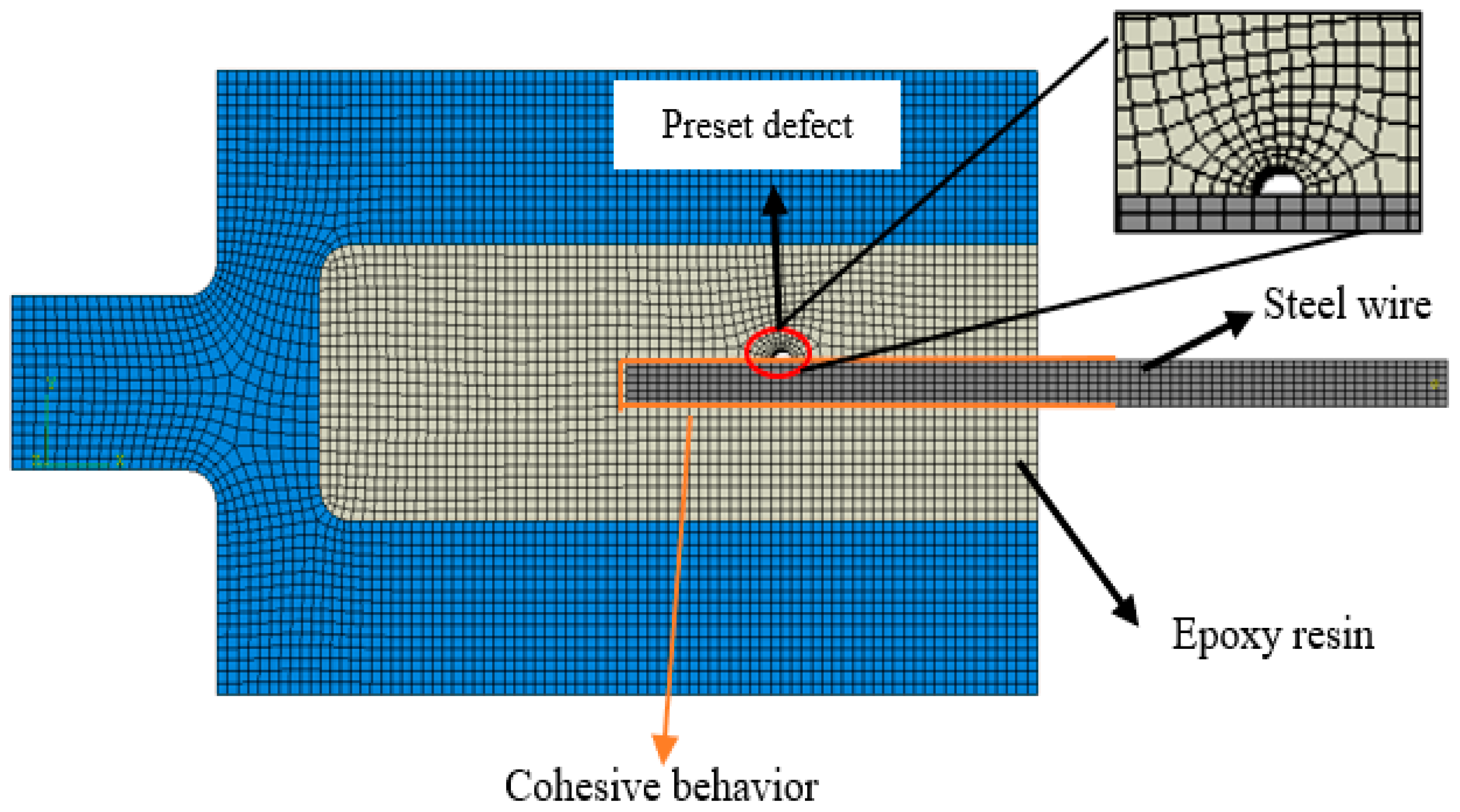
Finite element analysis (FEA) using the cohesive zone model (CZM) validates the revised parameterization, with errors between experimental and numerical results ranging from 3.0% to 7.2% (Table 2). Simulations confirm that $\lambda$ governs the effective load-transfer area and cohesive damage progression. Based on this, a revised critical defect threshold is proposed:

• $\lambda <0.025$: Defect effects are negligible; high-strength adhesives (e.g., Araldite^® AV138) are optimal.
• $0.025<\lambda <0.05$: Moderate defect control or moderate-toughness adhesives (e.g., Araldite^® 2015) are recommended.
• $\lambda >0.05$: Strict defect avoidance or high-toughness adhesives (e.g., Sikaforce^® 7752) are required.

For instance, in offshore applications where defect inspection is challenging, specifying $\lambda <0.025$ ensures structural reliability without excessive manufacturing costs. Conversely, in high-risk environments, combining $\lambda$-based defect limits with high-toughness adhesives mitigates failure risks.

7. Conclusions

This study systematically investigated the debonding failure mechanism at the epoxy-resin–tensile-armor interface in flexible pipe end fittings through experimental and numerical approaches. By integrating advanced digital image correlation (DIC) technology and cohesive zone modeling (CZM), the research quantified the impact of defect geometry and adhesive properties on structural integrity, offering actionable insights for deepwater engineering applications. The key findings are summarized as follows:

• Load-displacement curves for bonded specimens with defects revealed that interfacial defects significantly degraded load-bearing capacity. For specimens with a short bond length (L = 40 mm) and a defect diameter D = 4 mm, the failure load decreased by 9.5%. A dimensionless parameter, the defect-size-to-bond-length ratio ($\lambda =D/2L$), was proposed to unify defect impact across geometries. The derived power-law model $\Delta P(\%)=170.6\cdot {\lambda }^{0.85}$ quantifies failure load reduction with exceptional precision, establishing a benchmark for defect tolerance evaluation in industrial settings.
• Full-field DIC measurements captured real-time strain localization and crack propagation at defect edges, revealing a strain concentration factor (SCF) as high as 3.2. Crack initiation occurred at the outer interface and advanced inward, with strain redistribution accelerating interfacial debonding. This breakthrough visualization technique overcomes traditional limitations, enabling engineers to monitor failure progression with unprecedented spatial resolution.
• The CZM-based finite element model demonstrated remarkable accuracy, with errors between experimental and simulated failure loads ranging from 3.0% to 7.2%. Simulations confirmed that λ governs effective load-transfer area and damage progression. Critical thresholds were identified: $\lambda <0.025$ indicates negligible defect impact while $\lambda >0.05$ necessitates strict defect control or high-toughness adhesives.
• Adhesive performance varied dramatically under defect conditions. For L = 60 mm and D = 4 mm defects, high-toughness adhesives (e.g., Sikaforce^® 7752) reduced the failure load by only 4.3%, outperforming brittle adhesives (e.g., Araldite^® AV138, 8.3% reduction). The material toughness factor $(\Gamma =G_{IC}/{\sigma }_f)$ enabled a universal formula ($\Delta P\left(\%\right)=264\cdot {\Gamma }^{-0.3}\cdot {\lambda }^{0.85}$) to optimize adhesive selection for strength–toughness balance.

In conclusion, this study systematically investigated the debonding failure mechanisms at the epoxy-resin–tensile-armor interface in flexible pipe end fittings through integrated experimental and numerical approaches. The combined use of tensile testing, digital image correlation (DIC), and cohesive zone modeling (CZM) provided a comprehensive understanding of how interfacial defects influence structural integrity. By analyzing strain evolution and crack propagation dynamics, the research elucidated the critical role of defect geometry and adhesive properties in governing failure behavior. The proposed dimensionless parameter and material toughness framework offer practical guidelines for optimizing manufacturing processes and adhesive selection. However, the simplified uniaxial loading setup does not fully replicate operational multi-axial stresses in helical end fittings, and DIC resolution constraints limited the explicit visualization of defect-edge strain gradients. Future work will extend the λ–Γ framework to multi-axial loading scenarios using helical specimens and integrate high-resolution imaging (e.g., micro-DIC) to resolve localized strain fields, validating defect tolerance thresholds in industrial-scale prototypes. These findings advance the design of robust end fittings for deepwater applications, emphasizing defect control and material performance enhancement to ensure structural reliability under operational loads.