Abstract
Taiwan is frequently affected by typhoons, which cause storm surges and wave impacts that damage sea dikes, resulting in overflow and subsequent flooding. Therefore, it is essential to analyze the damage to sea dikes caused by storm surges and wave impacts, leading to overflow, for effective coastal protection. This study employs the ADCIRC model coupled with the SWAN model to simulate storm surges and waves around Taiwan and develops a sea dike failure model that incorporates mechanisms for impact damage, run-up damage, and overflow calculation. To ensure model accuracy, three historical typhoon events were used for calibration and validation of the ADCIRC+SWAN model. The results show that the ADCIRC coupled with SWAN model can effectively simulate storm surges and waves during typhoons. Typhoon Soulik (2013) was simulated to examine a breach in the Tamsui Youchekou sea dike in northern Taiwan, and an uncertainty analysis was conducted using the Monte Carlo method and Bayesian theorem. The results indicate that when the compressive strength of the sea dike is reduced to 5% of its original strength, impact and run-up damage occur, leading to overflow. In the case of impact damage, the overflow volume due to the breach falls within a 95% confidence interval of 0.16 × 10⁶ m3 to 130 × 106 m3. For run-up damage, the 95% confidence interval for the overflow volume ranges from 0.16 × 10⁶ m3 to 639 × 106 m3. The ADCIRC+SWAN model is used to simulate storm surge and waves, incorporating impact damage and run-up damage mechanisms to represent concrete sea dike failure. This approach effectively models dike failure and calculates the resulting overflow.
1. Introduction
Taiwan is situated in the Pacific typhoon belt and frequently experiences the impacts of typhoons. The storm surges and waves generated by typhoons pose significant threats to the lives and property of coastal populations, making sea dikes critical protective structures. These dikes are directly affected by storm surges and waves, and when the forces exerted exceed the design strength of the sea dikes, breaches may occur. In recent years, the increasing intensity and frequency of typhoons due to extreme weather, alongside tsunami disasters triggered by earthquakes, have resulted in more frequent damage to sea dikes. For example, Typhoon Herb in 1996 caused damage to at least five sea dikes in western Taiwan, with the total damaged length exceeding 2000 m. Typhoon Nari in 2001 destroyed over 1500 m of sea dikes in northern Taiwan, and Typhoon Mindulle in 2004 damaged around 200 m of sea dikes in western Taiwan. Typhoon Haitang in 2005 caused damage to 4340 m of sea dikes, while Typhoon Sepat in 2007 damaged approximately 500 m of dike structures. According to statistics from the Water Resources Agency, Ministry of Economic Affairs [1], a total of 6754 m of sea dikes was damaged between 2010 and 2019.
Given the variation in types, materials, and sea conditions of sea dikes, no widely accepted method exists for calculating dike breaches. Current numerical simulations focus primarily on overflow and hydrodynamic characteristics following a breach, often modeling breaches by reducing the dike crest height. Additionally, uncertainties in simulating typhoon-induced storm surges and waves further complicate the understanding of sea dike failure mechanisms. Therefore, this study applies uncertainty analysis to assess the potential extent of sea dike damage and overflow resulting from typhoon events.
Various models have been developed to simulate typhoon-induced storm surges and waves, each possessing distinct characteristics and limitations that render them suitable for specific applications. The primary models for storm surge simulation include SLOSH (Sea, Lake, and Overland Surges from Hurricanes), ADCIRC (ADvanced CIRCulation), and SCHISM (Semi-implicit Cross-scale Hydroscience Integrated System Model). The SLOSH model, developed by the U.S. National Weather Service in the 1990s (official website: https://vlab.noaa.gov/web/mdl/slosh, accessed on 12 March 2025), remains in use by the National Hurricane Center due to its computational efficiency [2,3]. SCHISM (http://ccrm.vims.edu/schismweb/, accessed on 5 January 2025), derived from SELFE, a semi-implicit Eulerian–Lagrangian finite-element model [4], incorporates enhancements such as extensions for large-scale eddy mechanisms and seamless cross-scale capability from streams to oceans [5]. ADCIRC, developed in 1992 by Dr. Luettich at the University of North Carolina (https://adcirc.org/, accessed on 20 February 2025), utilizes a highly flexible mesh system and combines the Generalized Wave Continuity Equation (GWCE) with the momentum conservation equation to address related challenges [6].
Common wave models include SWAN (Simulating WAves Nearshore), WAM, and WAVEWATCH III. The SWAN model (https://swanmodel.sourceforge.io/, accessed on 20 February 2025) is widely used for predicting coastal waves [7,8,9,10,11]. Like other spectral wave models, SWAN represents wave evolution by parameterizing sources (e.g., wind), sinks (e.g., whitecapping, bottom friction, and depth-limited breaking), and resonance (e.g., wave–wave interactions). The WAM model (https://github.com/mywave/WAM, accessed on 10 January 2024), developed by the WAM Group in 1988, uses a basic transport equation to describe the evolution of the two-dimensional wave spectrum without special assumptions regarding spectral shape. As a result, WAM has been increasingly used to study wave variations [12,13,14]. WAVEWATCH III solves the random phase spectral action density balance equation for wave number and directional spectra. Recent advancements, such as hurricane–wave interaction physics and wave–bottom interaction physics, have made WAVEWATCH III increasingly attractive for wave simulations [15,16,17].
To simultaneously simulate storm surges and waves, this study uses the ADCIRC model coupled with SWAN to simulate typhoon-induced storm surges and waves. The ADCIRC+SWAN coupling method has been widely utilized and demonstrated to be reliable [18,19,20,21]. For instance, simulations in the Gulf of Mexico have shown that the model can accurately simulate extreme storm surges and waves. When compared to the observed maximum wave height of 2.69 m during a hurricane, the ADCIRC+SWAN model’s error was only 0.04 m [22]. The model has also been applied in the Bay of Bengal, where it was able to accurately predict storm surges and waves [23].
Failure modes of sea dikes include cracking, toppling, sliding, and crest collapse due to wave impact [24,25]. Most research focuses on failure modes but does not examine overflow after a breach [26,27,28,29]. Some studies combine storm surge or wave models to explore sea dike failure mechanisms under wind and wave conditions [30,31,32,33,34]. In these cases, waves cause the failure, while storm surges lead to overflow. Research has also focused on the hydrodynamic characteristics of waves [35,36,37], distinguishing between breaking [38,39,40] and non-breaking waves [41,42,43,44]. Whether waves break or not, the primary failure modes are impact damage and run-up damage [45,46,47]. The results indicate a strong correlation between run-up height and the Iribarren number, defined , where β, H, and L represent the beach slope, wave height, and wavelength, respectively. Additionally, wave pressure increases with steeper dike slopes.
In uncertainty analysis, the choice of methods must balance accuracy, computational cost, and application goals. Common approaches include Monte Carlo Simulation (MCS) and Bayesian inference, which are often used in hydrological analyses to reduce model parameter uncertainty and improve prediction reliability [48,49,50,51,52,53]. Recently, these methods have also been used to explore uncertainties in storm surge predictions and their effects on coastal risk management under climate change, including uncertainties related to tidal levels, wave conditions, and model parameters [54,55,56].
The literature review demonstrates that while simulation techniques for typhoon-induced storm surges and waves are well developed, uncertainties remain due to the impacts of climate change. Future storm surges and waves caused by typhoons will continue to present challenges. In studies of sea dike failure, most research has focused on earth dikes [25,26,30,31], with relatively little attention paid to concrete dikes. Differences in dike type and material lead to a wide range of parameter values in failure models, further contributing to uncertainty. The main goal of this study is to apply the ADCIRC coupled SWAN model to simulate storm surges and waves in Taiwan’s surrounding waters and to establish a coastal concrete sea dike failure model. An uncertainty analysis is incorporated to enhance the accuracy of damage assessments, specifically evaluating impact damage and run-up damage caused by typhoon events.
2. Materials and Methods
2.1. Study Area Description
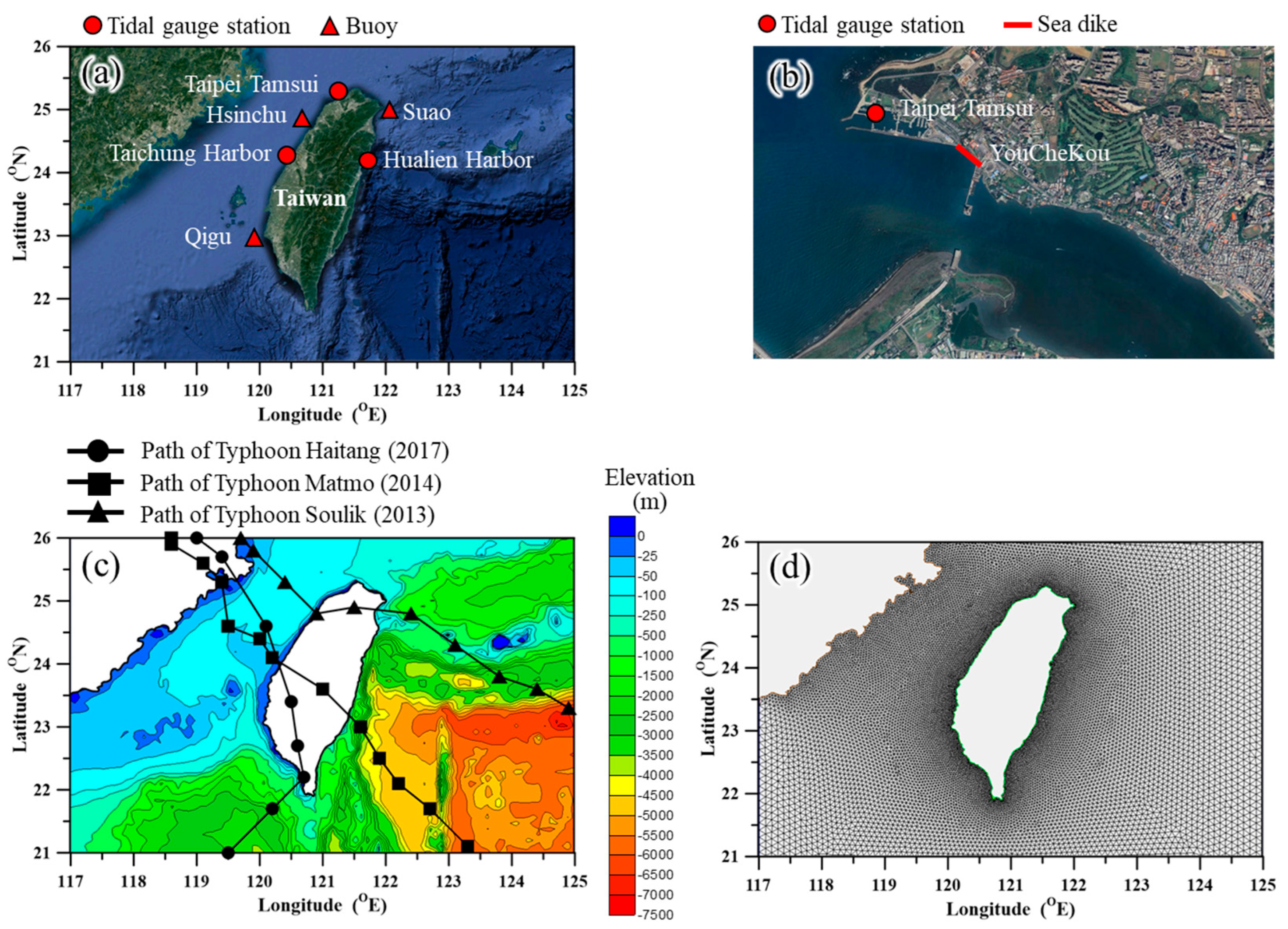
The sea dike section affected by overflow due to damage is situated in northern Taiwan. For calibration and validation of the ADCIRC+SWAN coupled model, tidal data from stations located at Taipei Tamsui, Taichung harbor, and Hualien harbor were used. Wave height data for calibration and validation were collected from the Suao, Hsinchu, and Qigu buoys (Figure 1a). The observational data were provided by the Central Weather Agency of Taiwan. This study focused on the Youchekou Dike on the right bank of the Tamsui River estuary (Figure 1b), with a total length of 461 m, a crest height of 5.57 m, and a front slope of 1:3.
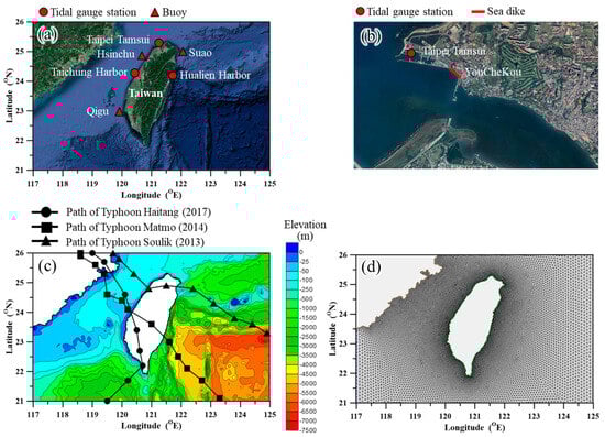
Figure 1.
Study area (a) tidal gauge and buoy stations, (b) location of YouCheKou dike, (c) path of typhoons and bathymetry around Taiwan, and (d) unstructured grids for ADCIRC+SWAN model.
Two typhoons, Soulik (2013) and Matmo (2014), were used for calibration, while Haitang (2017) was used for validation. Typhoon Soulik (2013) was further analyzed to assess uncertainty in overflow due to sea dike failure. Typhoon data, including central coordinates, central pressure, and maximum wind speed near the center, were sourced from the Central Weather Agency of Taiwan. Typhoon Soulik made landfall in northern Taiwan from the east and exited through the west. Typhoon Matmo entered central Taiwan from the east and exited from the west, while Typhoon Haitang approached southern Taiwan from the west and followed an arc-shaped path through central Taiwan (Figure 1c).
Topographic data for the ADCIRC+SWAN model were provided by the Ocean Science Center of the National Science Council (Figure 1c). The model utilized an unstructured triangular mesh consisting of 9560 nodes and 18,543 elements, with 200 offshore boundary nodes spaced approximately 20 km apart and 300 land boundary nodes along the Taiwan coast, spaced roughly 2 km apart (Figure 1d).
2.2. Typhoon Model
Storm surges during typhoons are primarily driven by the inverted barometric effect due to low pressure at the typhoon’s center, as well as wind shear acting on the sea surface. These forces are the primary mechanisms in storm surge models. To model the pressure and wind fields generated during typhoon events, this study employed a parameterized circular typhoon pressure empirical formula [2].
Accurate simulation of typhoon wind and atmospheric pressure fields is essential for applying the ADCIRC+SWAN model to simulate storm surges and waves during typhoon events. The parametric typhoon model provides a simple and efficient method for generating these wind and pressure fields. Compared to other typhoon models, its primary advantage is that it requires less input data and is straightforward to implement [57]. In this study, the atmospheric pressure field is modeled using the equation developed by [2], while the wind field follows the approach of [58]. The equations for the pressure field are as follows:
where ΔP= P∞ − P0; P∞ denotes the peripheral atmospheric pressure of the typhoon, P0 expresses the central atmospheric pressure of the typhoon, r represents the distance from any point to the typhoon center, and R is the radius of maximum wind (RMW).
The RMW can be calculated using the following equation [59]:
where φ denotes the latitude of the typhoon center, and Vf expresses the forward speed of the typhoon.
Young and Sobey [58] proposed that the wind speed, Vw, at any location within the typhoon wind field is composed of two components: the rotational wind speed, Vr, and the translational wind speed, Vt. These are expressed by the following equations:
where denotes the angle between the radial arm of the typhoon and the line of maximum winds.
2.3. Storm Surge and Wave Model
2.3.1. ADCIRC Model v52
ADCIRC (Advanced Circulation Model) is a finite-element model developed by Luettich et al. [60]. It is particularly suitable for simulating storm surges over large-scale offshore areas due to its flexible grid system, which allows for an unstructured mesh that can adapt to complex boundary shapes. The model can be driven by surface elevation at open boundaries and is set to no flux at land boundaries. Additionally, boundary conditions can be defined to accommodate time- and space-varying wind and pressure fields. At the land–sea interface, the model can simulate wetting and drying processes caused by tides.
When simulating tides with the ADCIRC model, it is necessary to input tidal parameters at the open boundaries. These parameters are obtained through the TOPEX/Poseidon Global Inverse Solution (v7.2), a global ocean tidal model developed by Oregon State University. This model provides the tidal height for each location and time, and it also offers the amplitude and phase angles for multiple tidal constituents, including M2, N2, S2, K1, and O1.
This study adopts a quadratic bottom friction law. For sandy seabeds, the quadratic friction coefficient typically ranges between 0.002 and 0.004 [61]. The model employs a Smagorinsky closure scheme with an eddy viscosity of 20 m2/s, and the initial wind stress parameter (TAU0) is set to 0.02. The model also utilizes variable Coriolis force (NCOR = 1), activates tidal forcing (NTIP = 1), and enables the terrain slope option (NRAMP = 1). The simulation time step is set to 20 s.
2.3.2. SWAN Model v41.31
The wave model used in this study is SWAN (Simulating WAves Nearshore), developed by Delft University of Technology. SWAN calculates wave propagation in both time and space domains, accounting for nonlinear wave–wave interactions, wave growth by wind, wave breaking, energy dissipation due to bottom friction, frequency shifts caused by currents and bathymetric changes, and processes such as shoaling and refraction. This makes it particularly effective for nearshore wave predictions [62]. SWAN uses a wave action density spectrum, defined as , where σ denotes the relative frequency and θ represents the wave direction. However, studies indicate that SWAN tends to underestimate wave height and period in the absence of background wind fields for wave energy [63]. Additionally, it does not account for advective and microturbulent transport in the vertical direction in coastal areas and may fail to accurately predict short-distance wave growth when spatial resolution is insufficiently refined [64,65].
The coupling between SWAN and ADCIRC is achieved by sharing the same unstructured finite element mesh. Initially, ADCIRC computes wind fields, water levels, and velocities at each mesh node. These outputs are then passed to SWAN, which solves the wave action density balance equation to obtain the wave spectrum for each node. The radiation stress caused by surface gravity waves [66] is then passed back to ADCIRC to update water levels and velocities for the next time step [67].
In SWAN, the wind input parameters based on [68] are used along with the whitecapping dissipation formula. Key settings include a whitecap dissipation rate (Cds2) of 4.5, a Pierson–Moskowitz spectrum slope parameter (Stpm) of 0.00302, a normalized slope parameter (Powst) of 4.0, and coefficients Delta and Powk both set to 1.0. The settings of these parameters are the default values of the model.
2.4. Sea Dike Failure Model
This study does not include physical model experiments, making it challenging to directly validate the failure mechanisms of concrete sea dikes. Instead, the reasonableness of impact damage and run-up damage mechanisms can only be inferred based on the physical principles embedded in the equations.
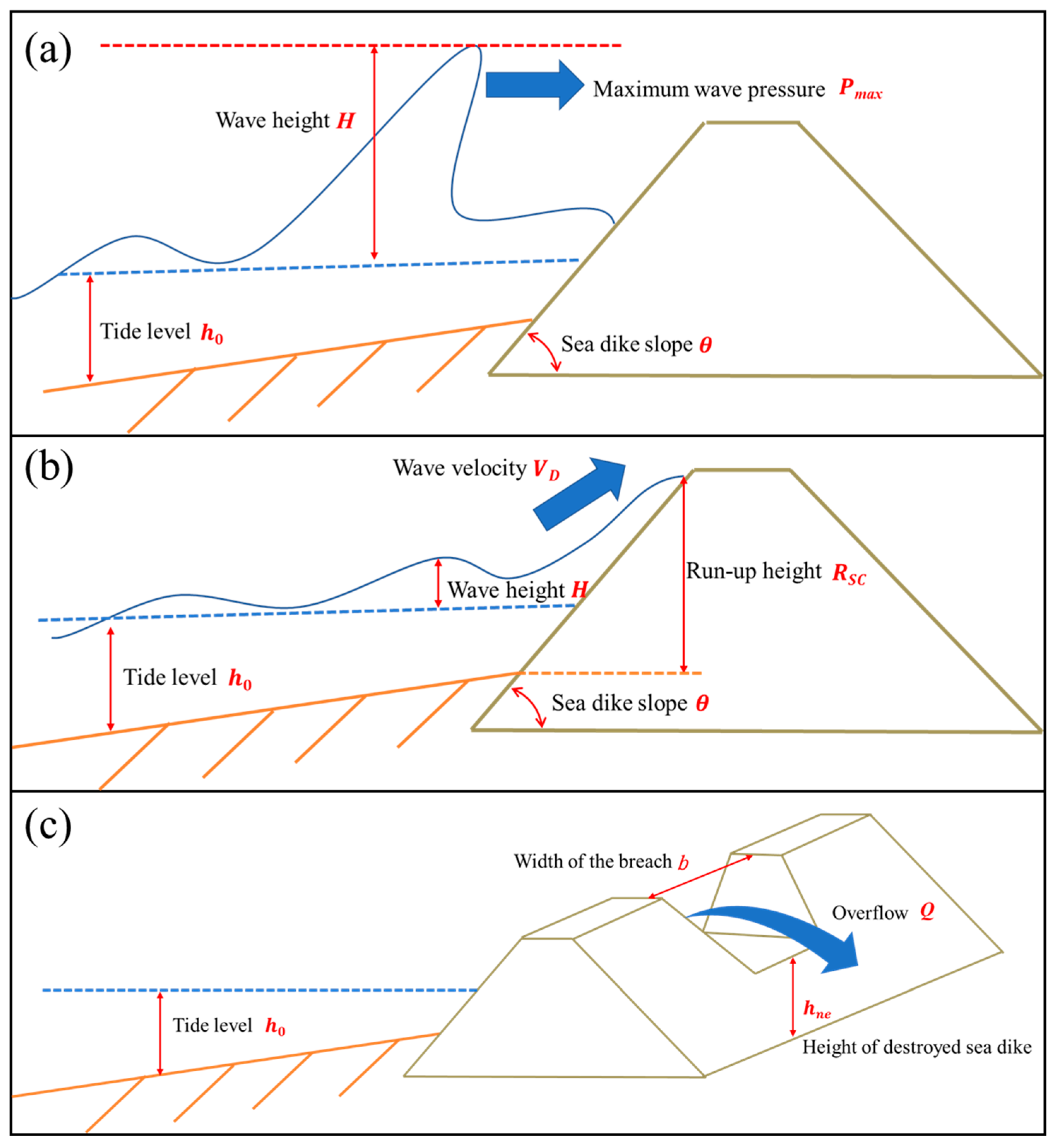
Impact damage occurs when wave pressure exceeds the compressive strength of the offshore flat-incline concrete sea dike (Figure 2a). For sea dikes, the compressive strength is 210 kgf/cm2, or 20,600 kN/m2. The maximum wave pressure (Pmax) is determined following the method described by McGovern et al. [69] (see Equation (9)). Equation (9) holds for obstacles with a vertical face. For sea dikes with inclined surfaces, the impact wave pressure can be adjusted using the Hoshiyama wave pressure formula [70] (see Equation (10)).
where is the maximum wave pressure (kN/m2), γ denotes a coefficient between 1.2 and 100 [71,72], ρ expresses the seawater density (ton/m3), g is gravitational acceleration (m/s2), H is wave height (m), expresses the maximum wave force acting on the inclined surface (kN/m2), represents the correction coefficient for the wave force acting on the slope, selected as the smaller of and , denotes the slope of sea dike (degrees), and L is the wavelength (m). When exceeds the compressive strength of concrete, the sea dike fails. The height of the breach ( can be expressed as
where is a coefficient equal to the compressive strength of concrete (0.05Ccs kN/m2) divided by the maximum wave force acting on the inclined surface and expresses the compressive strength of concrete (kN/m2). Because the compressive strength of concrete is always greater than the maximum wave force (FsH), impact damage will only occur when the compressive strength of concrete is reduced to 5%.
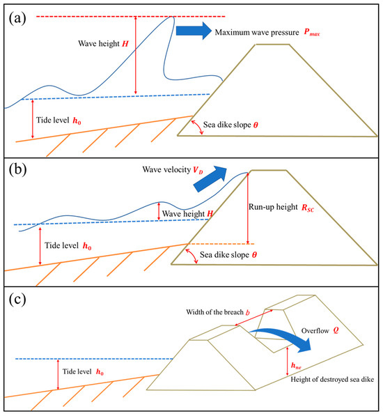
Figure 2.
Diagram of sea dike damage (a) impact damage, (b) run-up damage, and (c) breach overflow.
The run-up height (Figure 2b) is determined using the method outlined by [73] (see Equation (15)) to calculate .
where denotes the run-up height (m), α and β are coefficients, H expresses the wave height (m), and is defined by [73] Equation (16):
where denotes the slope of sea dike (degrees), and expresses the tide level (m).
Run-up damage occurs when the first wave reaches the run-up height, and the second wave collides with the receding first wave, creating suction that damages the sea dike slope. The wave travel distance along the sea dike slope is represented by x cot The time required for the wave to reach the run-up height is determined by dividing this travel distance by the wave velocity on the slope, with equal to 0 at this moment. Upon reaching the run-up height, the wave retreats along the slope back to the ocean. Since the travel distance remains unchanged, the retreat time equals the ascent time, which is twice the travel distance divided by the wave velocity on the slope. At this moment, equals 1. The time (T2) for the wave to reach the run-up height and retreat is calculated using Equation (17).
where VD denotes the wave velocity (m/s) and is a coefficient which ranges between 0 and 1. When the time T2 approaches the wave period T1, it indicates that the retreating first wave will intersect with the incoming second wave. This collision point can result in damage, defining the failure height of the sea dike as given in Equation (18).
In model calculations, achieving exact equality between T1 and T2 is challenging due to computational precision, which may introduce minor differences beyond the decimal point. Therefore, this study defines damage occurrence when the wave period T1 ranges between 0.9 and 1.1 times T2.
Once the sea dike breach height is determined from impact and run-up damage, the overflow volume can be calculated using the formula from [74] (see Figure 2c and Equation (19)).
where Q expresses the overflow volume (m3/s) and b is the width of the breach (m).
2.5. Statistical Error Analysis
The performance of the ADCIRC+SWAN model in simulating water levels and wave heights was evaluated using three metrics: root mean squared error (RMSE), dimensionless bias (DB) [75], and the Skill model [76]. The corresponding formulas are provided below:
where Oi represents the observed data, denotes the mean of the observed data, Si refers to the simulated data, and N is the number of data points. For RMSE and DB, lower values indicate a closer alignment between the model’s simulations and the observed data. A Skill metric closer to 1 reflects higher model accuracy. The Kolmogorov–Smirnov test (KS) [77] and the Akaike Information Criterion (AIC) [78] are used to assess the goodness of fit and identify the most suitable parameter distribution functions.
where x denotes the parameter value, expresses the sample cumulative distribution function, represents the compared cumulative distribution function, and is the degree of freedom (i.e., the number of parameters in the distribution function). The smaller the KS and AIC values, the closer the distribution function is to the sample distribution. Furthermore, in the analysis of the optimal number of groups for uncertainty analysis, the root mean square (RMS) and estimation uncertainty confidence interval (ECI) are utilized to evaluate the simulation results [79,80].
where OFi denotes the overflow (m3/h) in the ith simulation and OF5% and OF95% represent the 5th and 95th percentiles of all the simulated overflow, respectively. Once stable values for the RMS and ECI are obtained, an appropriate number of simulations or samples can be determined.
2.6. Research Outline
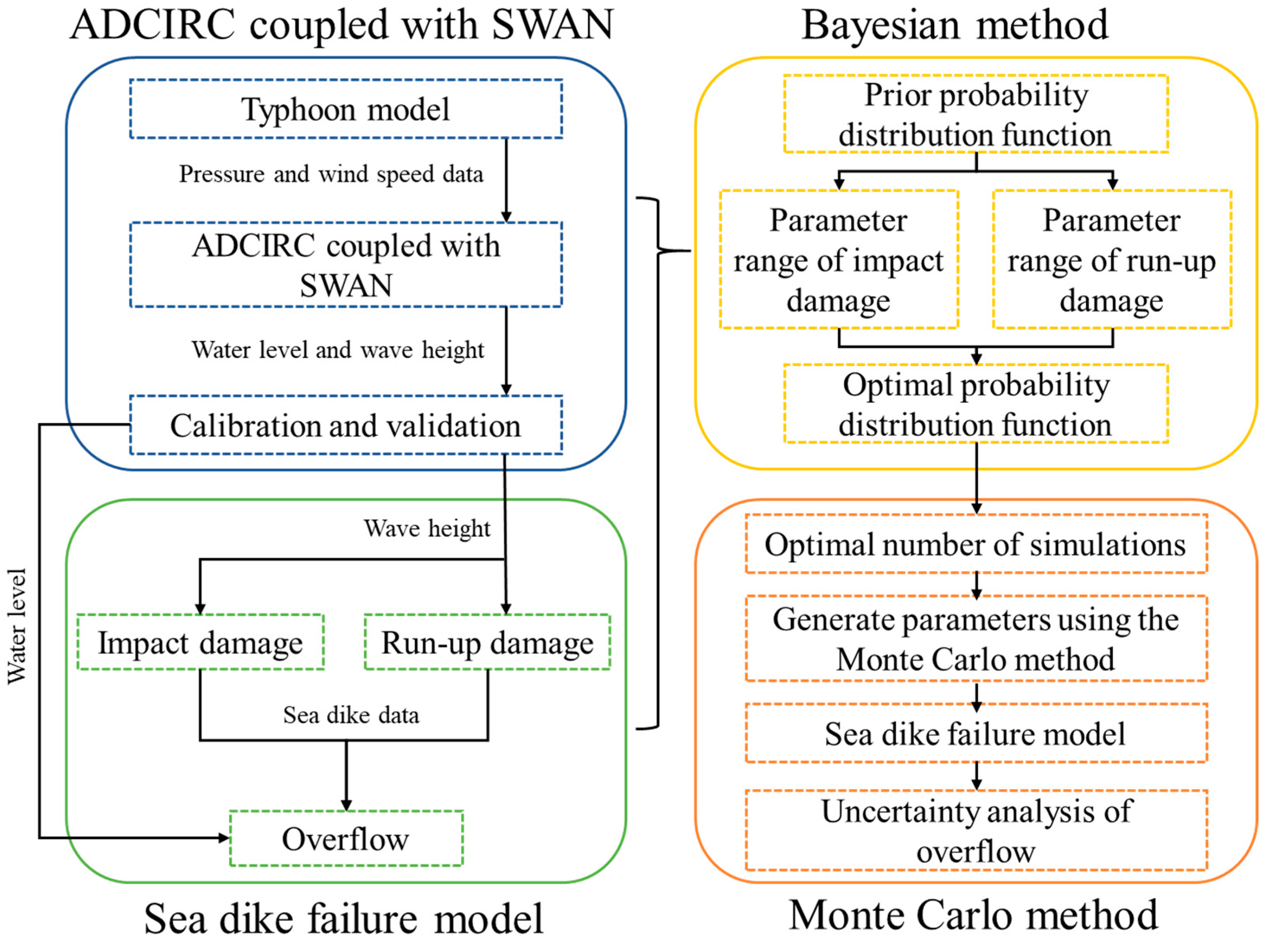
The research outline of this study is presented in Figure 3. The research outline is divided into four parts: ADCIRC coupled with SWAN, sea dike failure model, Bayesian method, and Monte Carlo method. In ADCIRC coupled with SWAN, the typhoon model generates wind speed and pressure field data, which serve as input for the ADCIRC model, coupled with the SWAN model. Calibration and validation of the ADCIRC+SWAN model were conducted using water level and wave height data from three historical typhoon events: Typhoon Soulik (2013), Typhoon Matmo (2014), and Typhoon Haitang (2017). After validation, the ADCIRC+SWAN model provides hourly water levels, wave heights, wave periods, and wave currents, which are used as inputs for the sea dike failure model.
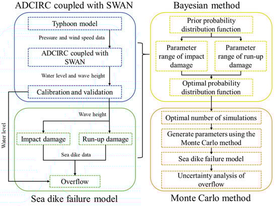
Figure 3.
Schematic representation of the research outline.
A concrete sea dike failure model is developed in this study, incorporating mechanisms for run-up damage, impact damage, and overflow calculations. When the wave height is below the dike height, the model determines the likelihood of run-up damage, while impact damage is calculated when the wave height exceeds the dike height. When the sea dike fails, the tidal water level and sea dike height are compared. If the tide water level is greater than the sea dike height, the overflow volume is calculated.
In the next step, the Bayesian method and Monte Carlo simulation are employed to evaluate the uncertainty associated with overflow due to sea dike failure. The Bayesian method is utilized to establish parameter ranges for run-up and impact damage mechanisms, ensuring a precise representation of dike failure. Simultaneously, the optimal probability distribution functions for these parameters are determined.
In the Monte Carlo method, the optimal number of simulations refers to the threshold below which the results of the probability distribution functions become unstable, with different numbers of simulations potentially producing varying distribution functions. To address this, this study first determines the optimal number of simulations and then applies Monte Carlo random sampling to select parameters for run-up and impact damages, assessing the uncertainty in sea dike failure and overflow. In this study, run-up damage and impact damage leading to sea dike failure during typhoon events are analyzed separately rather than in combination. If both failure mechanisms were simulated simultaneously, a single typhoon event might result in either impact damage or run-up damage, rather than capturing their potential coexistence.
3. Results
3.1. Storm Surge and Wave Model Calibration and Validation
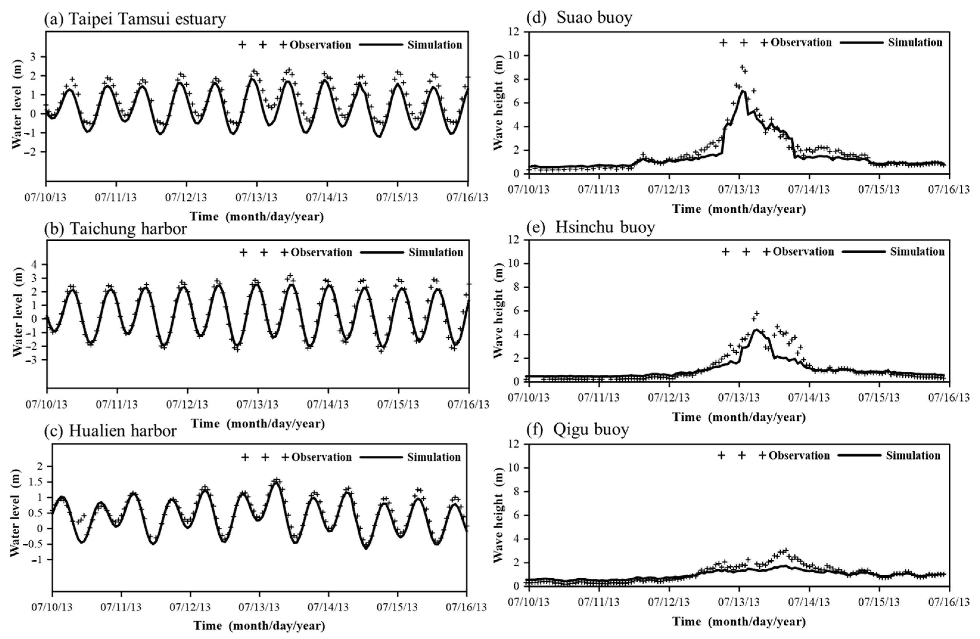
This study employed three typhoon events to calibrate and validate the storm surge and wave models. Observed water levels at Taipei Tamsui estuary, Taichung harbor, and Hualien harbor were compared with the simulated water levels, while observed wave heights from Suao buoy, Hsinchu buoy, and Qigu buoy were compared with the corresponding simulated wave heights. The parameters used in the ADCIRC and SWAN models for this study are detailed in Section 2.3.1 and Section 2.3.2. Calibration results for Typhoon Soulik (2013) and Typhoon Matmo (2014) are illustrated in Figure 4 and Figure 5, respectively, while validation results for Typhoon Haitang (2017) are presented in Figure 6.
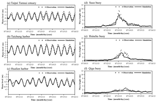
Figure 4.
Comparison of simulated and observed water levels at (a) Taipei Tamsui estuary, (b) Taichung harbor, and (c) Hualien harbor and wave heights at (d) Suao buoy, (e) Hsinchu buoy, and (f) Qigu buoy for Typhoon Soulik (2013).
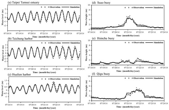
Figure 5.
Comparison of simulated and observed water levels at (a) Taipei Tamsui estuary, (b) Taichung harbor, and (c) Hualien harbor and wave heights at (d) Suao buoy, (e) Hsinchu buoy, and (f) Qigu buoy for Typhoon Matmo (2014).

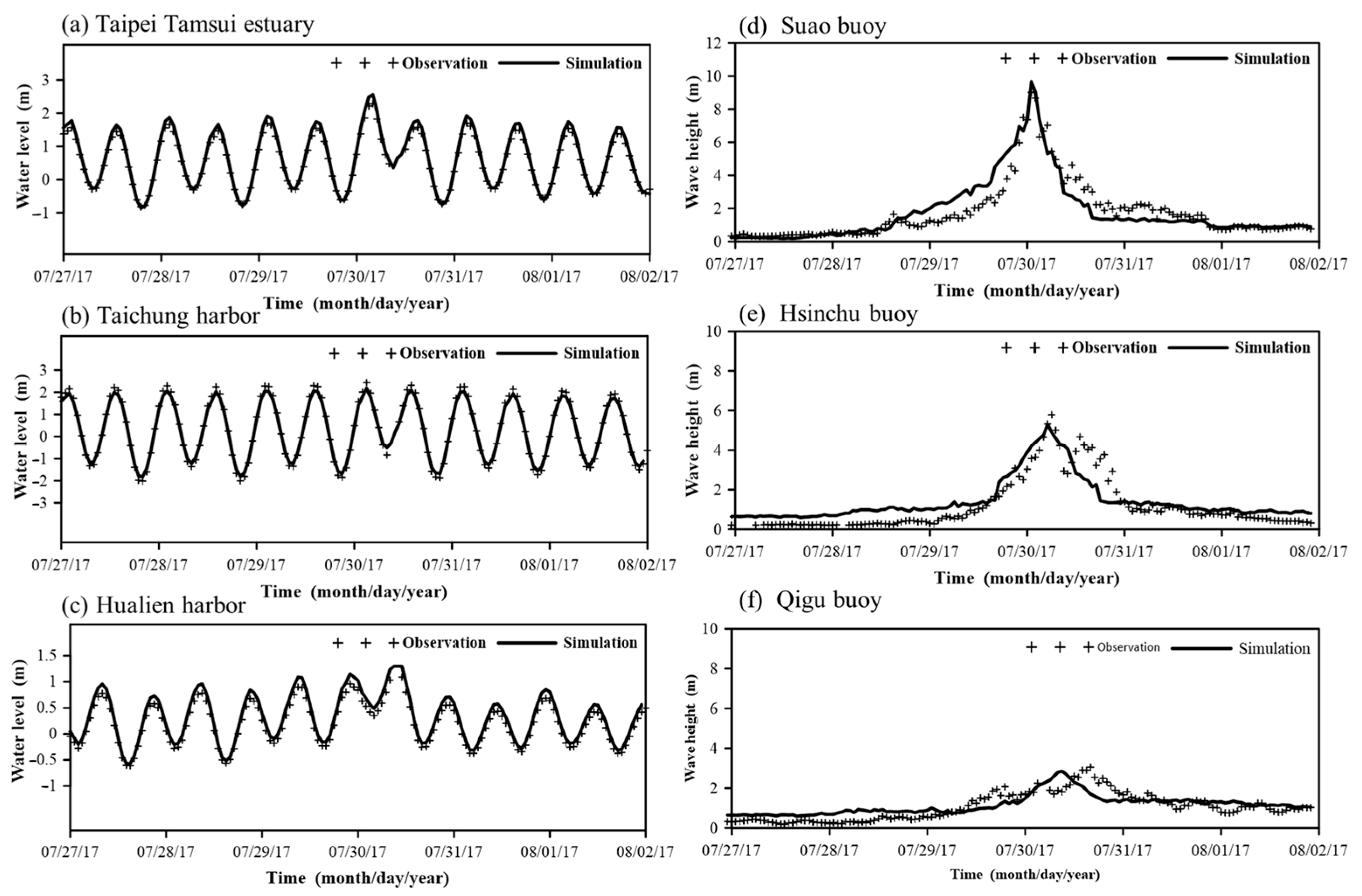
Figure 6.
Comparison of simulated and observed water levels at (a) Taipei Tamsui estuary, (b) Taichung harbor, and (c) Hualien harbor and wave heights at (d) Suao buoy, (e) Hsinchu buoy, and (f) Qigu buoy for Typhoon Haitang (2017).
The statistical errors obtained from the calibration and validation of the three typhoon events are summarized in Table 1. For water levels, the RMSE ranged from 0.11 m to 0.35 m, the DB varied between −0.39 and 0.23, and the Skill score ranged from 0.92 to 0.99. Similarly, for wave heights, the RMSE ranged from 0.21 m to 0.37 m, the DB varied between −0.11 and 0.21, and the Skill score ranged from 0.88 to 0.95. The findings demonstrate that the ADCIRC model, coupled with SWAN, effectively simulates water levels and wave heights along Taiwan’s coastal regions. Furthermore, the results confirm the reasonableness of the parameter values used in the ADCIRC and SWAN models.

Table 1.
Statistical errors for model calibration and validation across various typhoon events.
3.2. Sensitivity Analysis of Sea Dike Failure Model Parameters
Typhoon Soulik (2013), which made landfall in Taiwan as a severe typhoon, had a path closely aligned with the sea dike location under study. Therefore, this event was used to analyze the impact and run-up damage on the sea dike. In the sea dike failure model, key parameters were set to their maximum values: for impact damage, parameters γ and λSH were set to 100 and 1.2, respectively, while for run-up damage, parameters α and β were set to 0.2 and 2.0, respectively. Additionally, concrete strength was reduced to 5% of its original value.
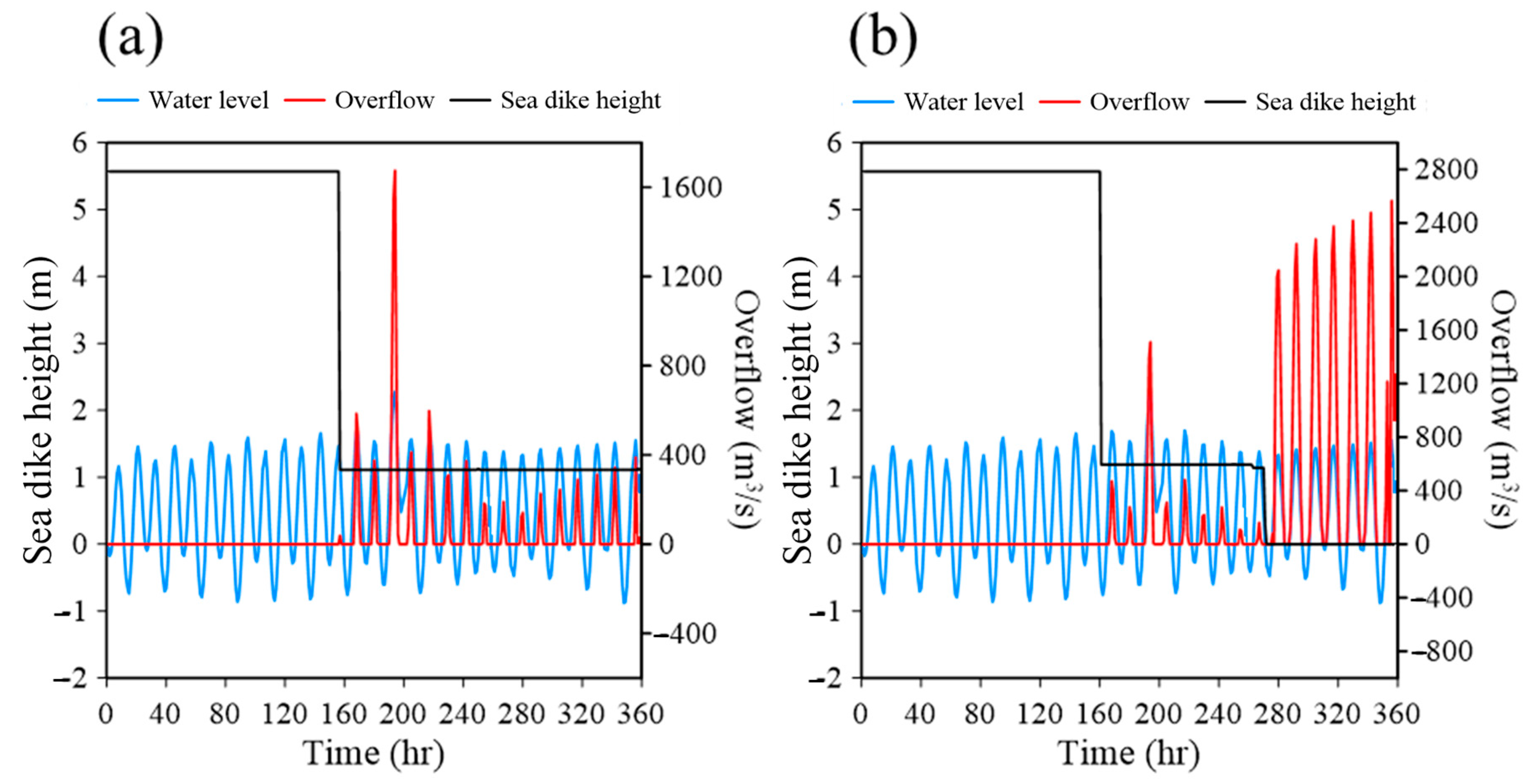
The simulation results are presented in Figure 7. The blue line shows the simulated water level, the red line indicates overflow, and the black line represents sea dike height. Figure 7a,b illustrate the impact and run-up damage, respectively. In Figure 7a, impact damage is observed at the 152nd hour, reducing the sea dike height from 5.8 m to 1.2 m, which led to overflow when the water level surpassed the dike height. The highest storm surge level, recorded at the 198th hour, reached 2.1 m, resulting in a maximum overflow of 1600 m3/s. In Figure 7b, run-up damage occurs at the 162nd hour, lowering the dike height from 5.8 m to 1.4 m. A second run-up event happened at the 276th hour, reducing the dike height to 0 m, which led to overflow exceeding 2000 m3/s during high tide.
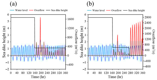
Figure 7.
Temporal variations in sea dike height and overflow during Typhoon Soulik (2013) (a) impact damage and (b) run-up damage.
A comparison of Figure 7a,b reveals that following the first dike failure due to impact damage at the 152nd hour, the subsequent decrease in wave height stabilized the dike height at 1.2 m, preventing further impact-induced failure. In contrast, for the run-up damage mechanism, the initial dike failure occurred at the 162nd hour. As the typhoon moved away and the wave period shortened, a second dike failure occurred at the 276th hour, ultimately reducing the dike height to 0 m. These findings suggest that, under certain conditions, run-up damage may pose a greater threat to dike stability than impact damage.
Figure 7 further illustrates the independence of the impact and run-up failure mechanisms during the simulation. The two mechanisms trigger dike failure at different times: impact failure causes the first dike failure at the 152nd hour (Figure 7a), whereas run-up failure induces the first dike failure at the 162nd hour (Figure 7b). Additionally, while run-up failure leads to a second dike failure at the 276th hour, impact failure does not result in a subsequent failure event.
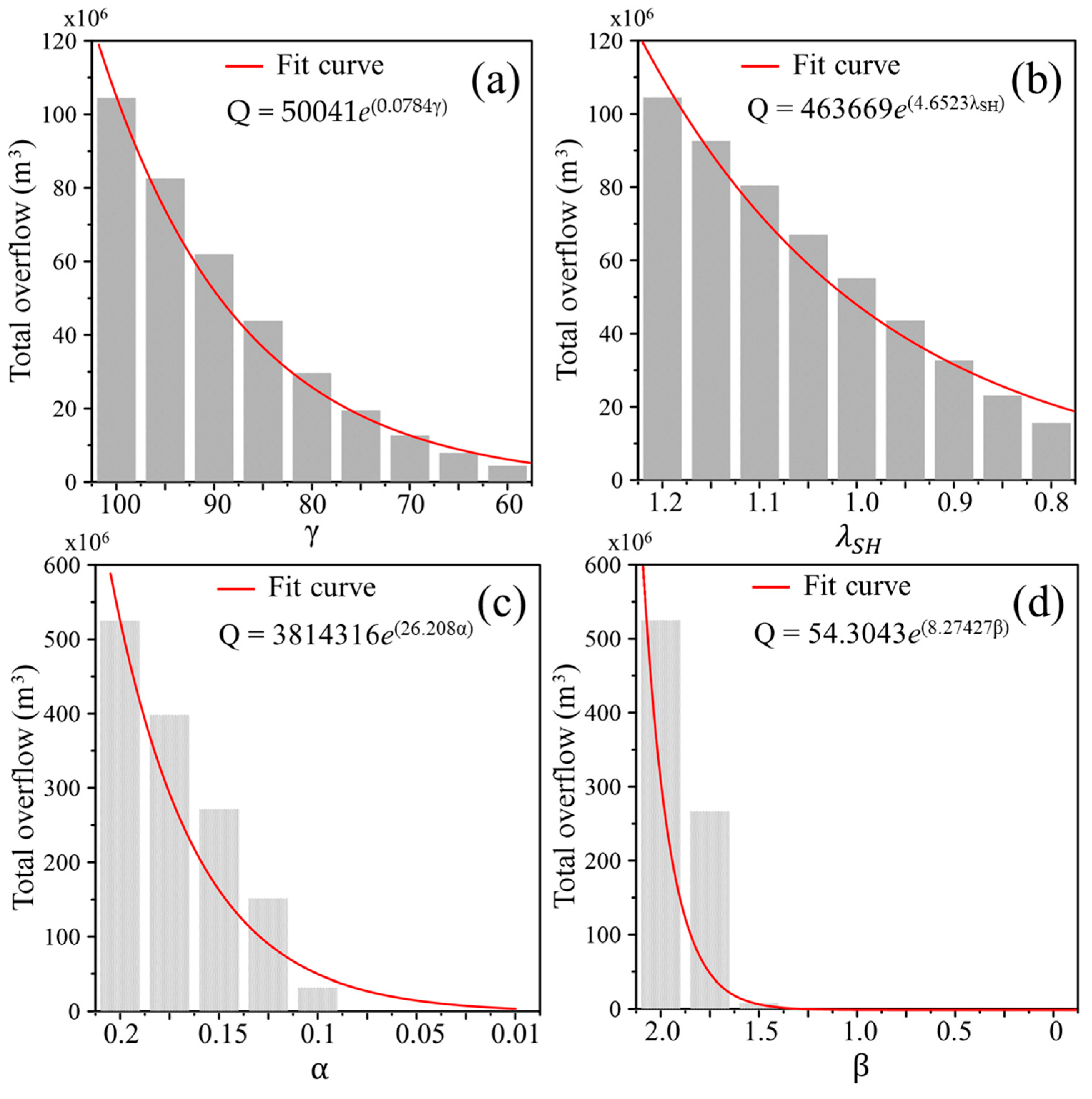
For uncertainty analysis of overflow following dike failure, the Bayesian method was used to determine parameter ranges for the impact and run-up damage mechanisms. The Typhoon Soulik event served as the basis for the analysis, and results are shown in Figure 8. Figure 8a demonstrates that no overflow occurs for the impact damage mechanism when parameter γ is below 60 and λSH is set to 1.2. When γ reaches 100, the overflow volume is approximately 104 × 106 m3. Additionally, when γ is set to 100 and λSH is between 0.8 and 1.2, overflow occurs (Figure 8b). The relationship between parameter γ and overflow can be expressed as Q = 50041e(0.0784γ), with a correlation coefficient (R) of 0.99. Similarly, the relationship between λSH and overflow is expressed as Q = 463669e(4.6523λSH), with a correlation coefficient of 0.98.
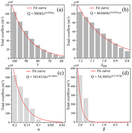
Figure 8.
Sensitivity analysis for sea dike failure model parameters: (a) γ and (b) λSH for impact damage and (c) α and (d) β for run-up damage parameters.
For the run-up damage mechanism, overflow occurs when parameter β is set to 2.0 and parameter α exceeds 0.1 (Figure 8c). Similarly, when parameter α is set to 0.2 and parameter β is greater than 1.5, overflow occurs (Figure 8d). When α is set to 0.2 and β to 2.0, the resulting overflow is 532 × 106 m3. The relationship between α and overflow is given by Q = 3814316e(26.208α), with a correlation coefficient (R) of 0.96, while the relationship between β and overflow is expressed as Q = 54.3043e(8.27427β), with an R of 0.96.
By applying the Bayesian method and sensitivity analysis, the parameter ranges for impact damage and run-up damage mechanisms can be determined. Additionally, the analysis reveals that although the parameter range for the run-up damage mechanism is narrower, it exhibits greater sensitivity than the impact damage mechanism, leading to increased overflow.
3.3. Uncertainty Analysis
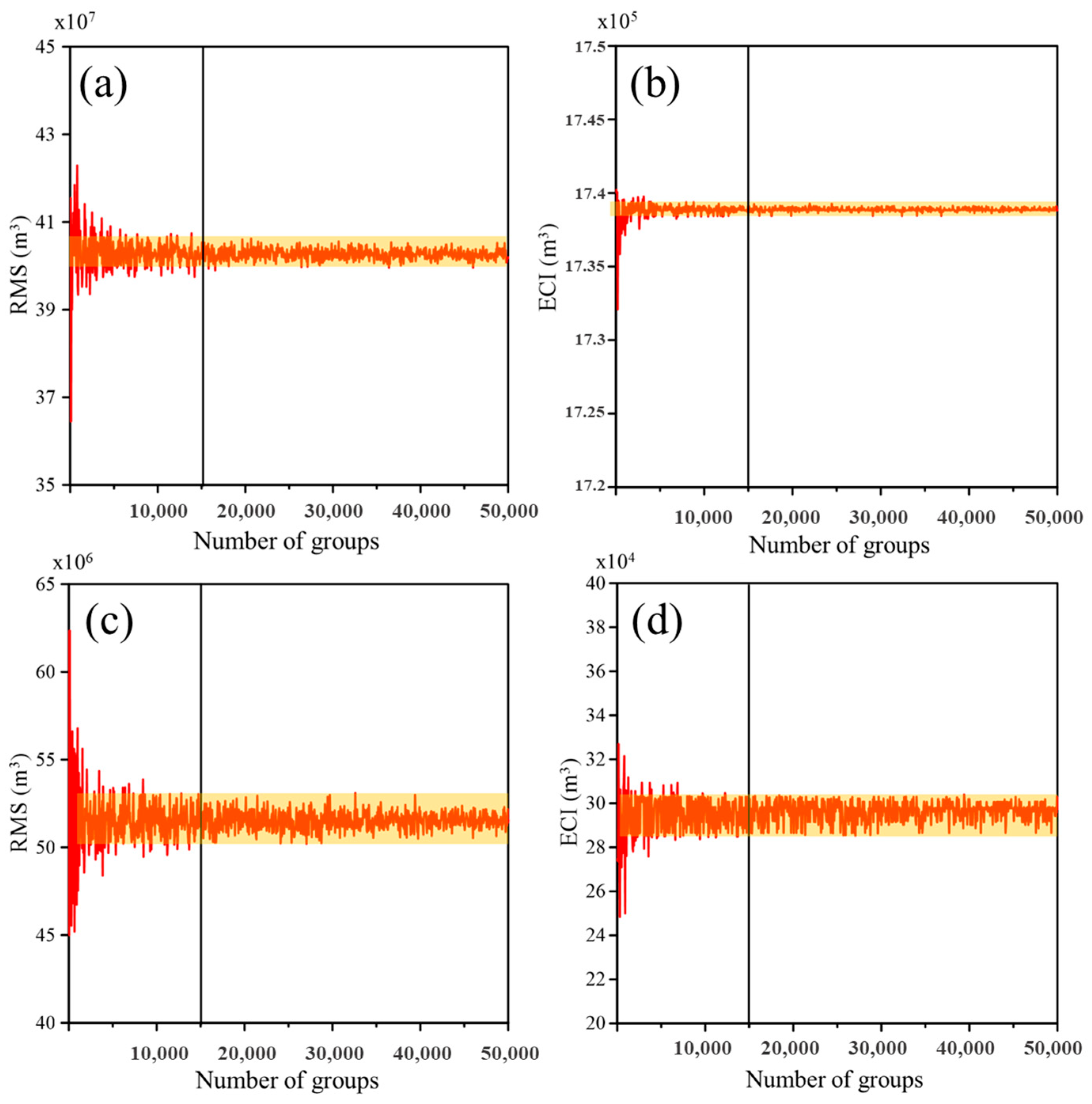
Prior to conducting uncertainty analysis using Monte Carlo and Bayesian methods, it was necessary to establish the optimal number of simulations and the parametric distribution functions. Determining the appropriate number of simulations is crucial to avoid either too few simulations, which could cause significant variability in results, or too many, which would waste computational resources. In this study, the variation in overflow caused by impact and run-up damages was assessed under different numbers of simulations using the RMS and ECI (Figure 9). Figure 9a,b present the number of simulations for impact damage, while Figure 9c,d display the number of simulations for run-up damage. The simulations stabilized after approximately 15,000 simulations, which were subsequently used for the uncertainty analysis.
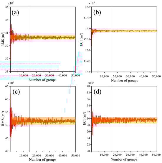
Figure 9.
Number of simulations for RMS and ECI indices: (a) γ and (b) λSH for impact damage parameters and (c) α and (d) β for run-up damage parameters.
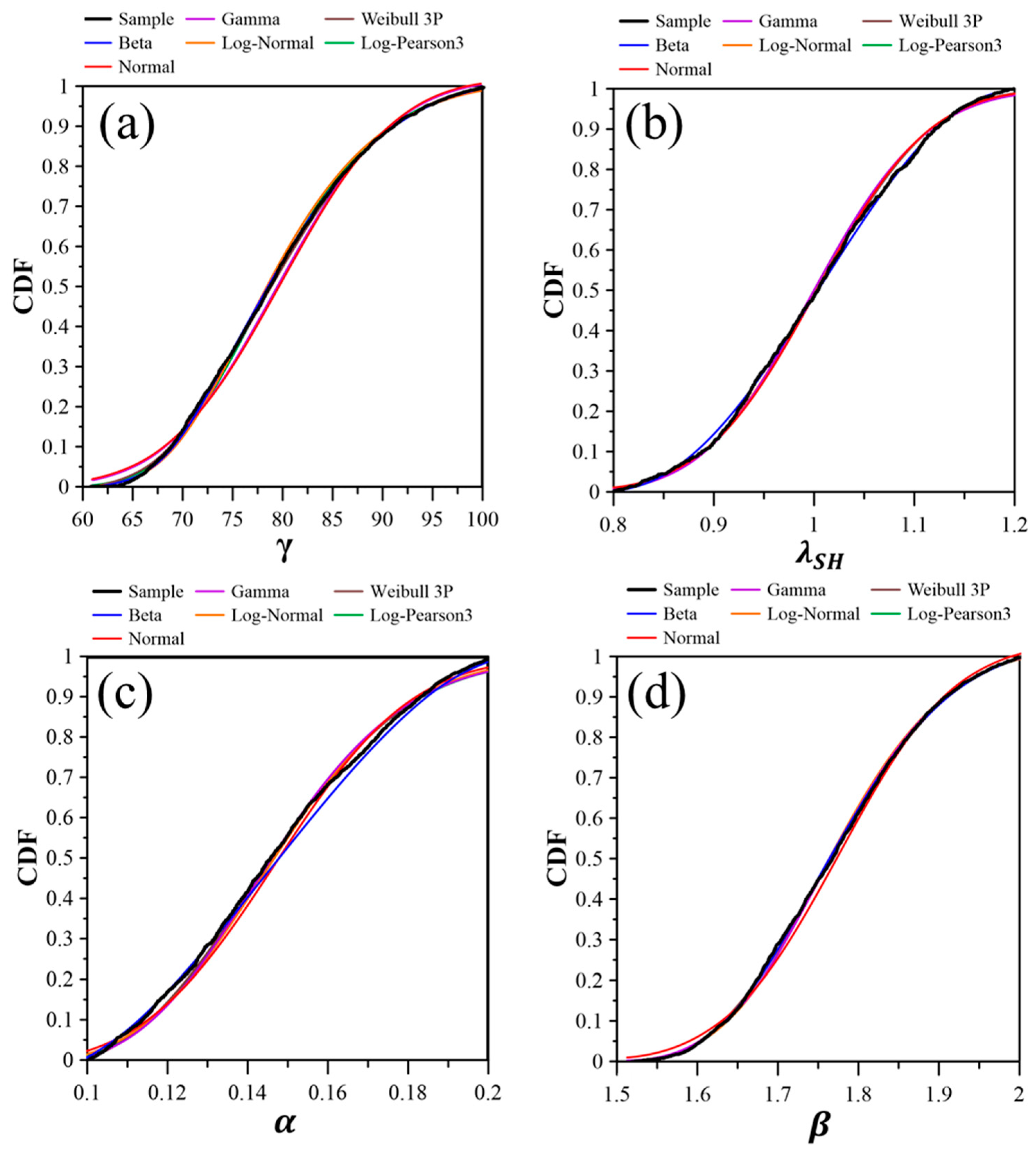
To identify the parameter distribution functions, six frequency functions were examined: Beta, Normal, Gamma, Lognormal, Weibull 3P, and Log-Pearson 3P. Parameters γ and λSH for impact damage (Figure 10a,b) and α and β for run-up damage (Figure 10c,d) were considered. The parameter samples were derived through the prior procedure of the Bayesian method, where initial parameter ranges for the impact and run-up damage mechanisms were assigned normal distribution functions. Through repeated sampling and evaluation of dike failure and overflow occurrence, the parameter ranges were refined, while simultaneously identifying the parameter samples that lead to dike failure and overflow. Figure 10 shows the cumulative distribution function (CDF) for six frequency functions across various parameters, demonstrating a close alignment with the sample distribution. Based on the fitness assessment using KS and AIC, the Beta distribution provided the best fit for γ and λSH, while the Weibull 3P distribution was optimal for α and β (Table 2).
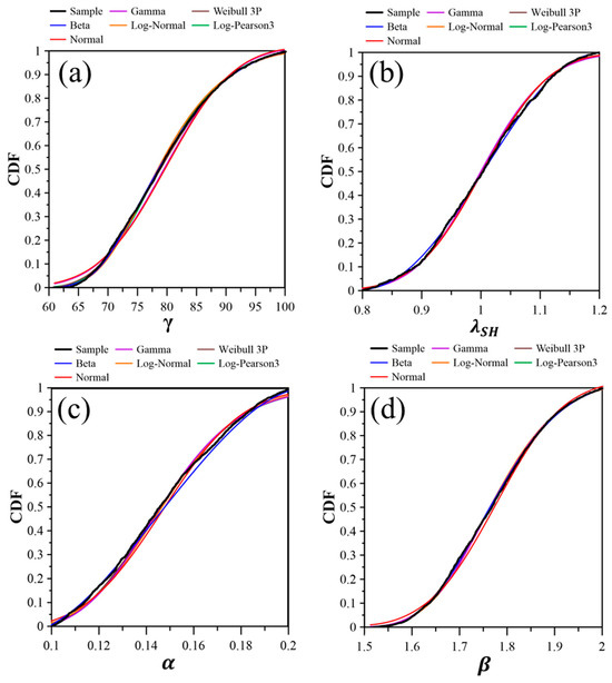
Figure 10.
Cumulative distribution functions (CDFs) for various frequency functions: (a) γ and (b) λSH for impact damage parameters and (c) α and (d) β for run-up damage parameters.
Table 2.
Statistical analysis of different frequency functions.
Based on the identified frequency functions, an uncertainty analysis of overflow due to impact and run-up damages was conducted using 15,000 simulations. Figure 11 presents the mean and the 95% confidence interval of the simulated overflow resulting from impact and run-up damages. Figure 11a shows that impact damage leads to overflow at the 152nd hour, and at the highest tide (198th hour), the overflow within the 95% confidence interval ranges from 0.13 × 10⁶ m3/h to 8 × 10⁶ m3/h, with an average of 3.8 × 10⁶ m3/h. The total overflow ranges from 0.16 × 10⁶ m3 to 130 × 106 m3, with an average of 26.77 × 10⁶ m3. Figure 11b depicts that run-up damage results in overflow at the 162nd hour, and at the highest tide (198th hour), the overflow ranges from 0.83 × 10⁶ m3/h to 16 × 106 m3/h, with an average of 7.2 × 10⁶ m3/h. The total overflow due to dike failure under the run-up damage model falls within 0.16 × 10⁶ m3 to 639 × 106 m3, with an average value of 323 × 106 m3.
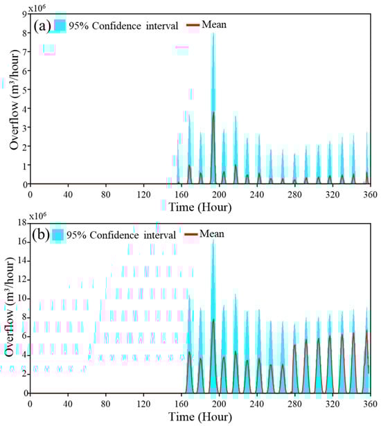
Figure 11.
Uncertainty analysis of temporal variations in overflow: (a) impact damage and (b) run-up damage.
4. Discussion
4.1. Novelty and Strength
Previous research on sea dike failure has primarily centered on laboratory experiments, with a focus on understanding the failure mechanisms of sea dikes [28,29,33,34]. However, there is a notable gap in studies addressing sea dike failures triggered by storm surges and waves generated during typhoon events, as well as the overflow resulting from these failures. This study bridges this gap by integrating a surge–wave model with a sea dike failure model to investigate these phenomena. The reliability of surge–wave models has been confirmed in several studies [20,21,22,23], while the formulas and parameters for the sea dike failure model are derived from previous research [69,70,71,72,73,74]. This research is pioneering in combining a surge–wave model with a sea dike failure model. The surge–wave model supplies accurate tidal and wave data to the sea dike failure model, which then assesses the likelihood of failure and performs uncertainty analysis on the overflow volume if failure occurs. The strength of this method lies in its ability to simulate sea dike failure and overflow during typhoon events without requiring the development of a new model that integrates storm surges, waves, dike failure, and overflow. By leveraging existing models and established failure mechanisms, the approach effectively simulates failure scenarios and conducts uncertainty analyses of the resulting overflow.
4.2. Limitations and Applicability
The model developed in this study has two primary limitations. First, in real-world scenarios, impact damage and run-up damage may occur simultaneously when waves strike a sea dike. Factors such as dike thickness and surface friction coefficient must be considered; however, accurately capturing these phenomena requires high-resolution numerical models, such as Smoothed Particle Hydrodynamics (SPH), Moving Particle Semi-Implicit (MPS), and OpenFOAM [26,46,81,82,83]. These models are typically constrained to small-scale regions and can only simulate the effects of a limited number of waves over short timeframes (minutes to hours). To analyze large-scale storm surges and waves and assess sea dike failure, computational limitations necessitate reducing spatial resolution and employing simplified classification methods to categorize waves before selecting the appropriate failure mechanism for analysis. This trade-off inevitably reduces simulation accuracy and may result in the underestimation of wave-induced dike failure.
Second, the model’s limited grid resolution restricts its ability to accurately simulate wave breaking in shallow water, potentially leading to an underestimation of wave height. To precisely capture shallow-water wave breaking, a grid resolution finer than 50 m is required [9,18]. However, achieving such resolution significantly increases computational demands and processing time, posing challenges to simulation efficiency.
The method proposed in this study has broad applicability, primarily because surge–wave coupling models are well established. In addition to the ADCIRC+SWAN coupled model, other storm surge models like SLOSH and SCHISM [3,5] and wave models like WAM and WAVEWATCH [14,16] can be used to simulate surge and wave data as inputs for the sea dike failure model. Developing the sea dike failure model requires additional programming, using failure mechanism equations from prior studies. The storm surge and wave data are inputted into the sea dike failure model to determine whether failure will occur and, if so, to predict the post-failure sea dike height. The assumption that storm surge and wave data are available allows for immediate calculation of sea dike failure and overflow volume. This method is therefore more practical and applicable for disaster prevention and response.
4.3. Future Work
Future research in this area can advance in three primary directions. First, it is essential to account for additional sea dike failure mechanisms such as overtopping, toppling, and sliding [24,25,33,84]. Second, the development of a comprehensive database of regional sea dikes could facilitate real-time failure analysis. For instance, in Taiwan, once additional failure mechanisms are incorporated and a complete sea dike database is in place, analyses of sea dike failure and overflow for the upcoming 15 days could be completed within 30 min. Third, the determination of sea dike strength parameters requires further investigation. As discussed in Section 3.2, standard-strength concrete sea dikes typically resist damage, yet prolonged exposure to weathering or insufficient maintenance can weaken them, increasing their vulnerability to storm surges and wave action. Accordingly, future studies should aim to establish suitable strength parameters for sea dikes, considering factors such as age and maintenance conditions.
5. Conclusions
This study employs the ADCIRC+SWAN coupled model to simulate storm surges and waves around Taiwan. Additionally, it integrates models for impact and run-up damage mechanisms on sea dikes to simulate overflow due to sea dike breaches. Uncertainties in overflow caused by dike failure are evaluated using Monte Carlo and Bayesian methods. Model calibration and validation were performed using three historical typhoon events. The results indicate that the RMSE between simulated and observed water levels is less than 0.35 m, with a DB ranging from −0.39 to 0.23 and a Skill score exceeding 0.92. Similarly, the RMSE for wave heights is below 0.37 m, with a DB ranging from −0.11 to 0.21 and a Skill score above 0.88. These findings confirm the model’s accuracy in simulating storm surges and waves around Taiwan.
Following validation, Typhoon Soulik (2013) was selected for sea dike failure analysis at the YouCheKou sea dike in Tamsui, northern Taiwan. The Bayesian method was applied to estimate parameter ranges for overflow due to impact and run-up damage. The impact damage parameter, γ, ranged from 60 to 100, and λSH ranged from 0.8 to 1.2. For run-up damage, α ranged from 0.1 to 0.2, while β ranged from 1.5 to 2.0. Monte Carlo simulations were used to determine the best probability distributions for these parameters. The Beta frequency function was identified as the best fit for γ and λSH, while the Weibull 3P frequency function best represented α and β. The RMS and ECI indices were employed to determine the optimal simulation count, set at 15,000. Subsequently, 15,000 sets of failure parameters were used to simulate sea dike damage and overflow. Under the worst-case scenario, the impact damage resulted in an overflow of 130 × 106 m3, while run-up damage caused an overflow of 639 × 106 m3.
This study demonstrates that the ADCIRC+SWAN coupled model, in combination with a sea dike failure mechanism model and uncertainty analysis, provides a viable approach for simulating storm surges, waves, and offshore flat-incline concrete sea dike breaches in Taiwan.
Author Contributions
Conceptualization, W.-C.L. and W.-C.H.; methodology, W.-C.H. and H.-M.L.; software, W.-C.H.; validation, W.-C.L., W.-C.H. and H.-M.L.; formal analysis, W.-C.H.; investigation, W.-C.L. and W.-C.H.; resources, W.-C.L.; data curation, W.-C.H. and H.-M.L.; writing—original draft preparation, W.-C.L. and W.-C.H.; writing—review and editing, W.-C.L. and H.-M.L.; visualization, W.-C.H. and H.-M.L.; supervision, W.-C.L.; project administration, W.-C.L. and W.-C.H.; funding acquisition, W.-C.L. All authors have read and agreed to the published version of the manuscript.
Funding
This research was funded by the National Science and Technology Council of Taiwan (NSTC) under grant no. 112-2625-M-239-001.
Institutional Review Board Statement
Not applicable.
Informed Consent Statement
Not applicable.
Data Availability Statement
Data are contained within the article.
Acknowledgments
The authors gratefully acknowledge the Central Weather Administration of Taiwan for supplying the observational data.
Conflicts of Interest
The authors declare no conflicts of interest.
References
- Water Resources Agency, Ministry of Economic Affairs. 2020 Water Resources Statistics of the Republic of China; Water Resources Agency, Ministry of Economic Affairs: Taipei City, Taiwan, 2020.
- Jelesnianski, C.P. A numerical calculation of storm tides induced by a tropical storm impinging on a continental shelf. Mon. Weather Rev. 1965, 93, 343–358. [Google Scholar] [CrossRef]
- Glahn, B.; Taylor, A.; Kurkowski, N.; Shaffer, W.A. The Role of the SLOSH model in national weather service storm surge forecasting. Natl. Weather Dig. 2009, 33, 3–14. [Google Scholar]
- Zhang, Y.; Baptista, A.M. SELFE: A semi-implicit Eulerian-Lagrangian finite-element model for cross-scale ocean circulation. Ocean Model. 2008, 21, 71–96. [Google Scholar] [CrossRef]
- Zhang, Y.; Ye, F.; Stanev, E.V.; Grashorn, S. Seamless cross-scale modeling with SCHISM. Ocean Model. 2016, 102, 64–81. [Google Scholar] [CrossRef]
- Westerink, J.J.; Luettich, R.A.; Blain, C.A.; Scheffner, N.W. ADCIRC: An Advanced Three-Dimensional Circulation Model for Shelves, Coasts and Estuaries; Report 2: Users’ Manual for ADCIRC-2DDI. Technical Report, DRP-94; U.S. Army Corps of Engineers: Wahington, DC, USA, 1994.
- Amarouche, K.; Akpinor, A.; Bachari, N.E.S.; Cakmak, R.E.; Houma, F. Evaluation of a high-resolution wave hindcast model SWAN for the West Mediterranean basin. Appl. Ocean Res. 2019, 84, 225–241. [Google Scholar] [CrossRef]
- Vieira, F.; Cavalcante, G.; Campos, E. Analysis of wave climate and trends in a semi-enclosed basin (Persian Gulf) using a validated SWAN model. Ocean Eng. 2020, 196, 106821. [Google Scholar] [CrossRef]
- Yan, J.; Rong, Z.; Li, P.; Qin, T.; Yu, X.; Chi, Y.; Gao, Z. Modeling waves over the Changjiang River Estuary using a high-resolution unstructured SWAN model. Ocean Model. 2022, 173, 102007. [Google Scholar]
- Rybalko, A.; Myslenkov, S. Analysis of current influence on the wind wave parameters in the Black Sea based on SWAN simulations. J. Ocean Eng. Mar. Energy 2023, 9, 145–163. [Google Scholar] [CrossRef]
- Jialei, L.; Shi, J.; Zhang, W.; Xia, J.; Wang, Q. Numerical simulations on waves in the Northwest Pacific Ocean based on SWAN models. J. Phys. Conf. Ser. 2023, 2486, 012034. [Google Scholar] [CrossRef]
- Foteinis, S.; Hancock, J.; Mazarakis, N.; Tsoutsos, T.; Synolakis, C.E. A comparative analysis of wave power in the nearshore by WAM estimates and in-situ (AWAC) measurements. The case study of Varkiza, Athens, Greece. Energy 2017, 138, 500–508. [Google Scholar] [CrossRef]
- Stathopoulos, C.; Galanis, G.; Kallos, G. A coupled modeling study of mechanical and thermodynamical air-ocean interface processes under sea storm conditions. Dyn. Atmos. Ocean. 2020, 91, 101140. [Google Scholar] [CrossRef]
- Bhavithra, R.S.; Sannasiraj, S.A. Climate change projection of wave climate due to Vardah cyclone in the Bay of Bengal. Dyn. Atmos. Ocean. 2022, 97, 101279. [Google Scholar] [CrossRef]
- Heo, K.Y.; Ha, T.; Park, K.S. The effects of a typhoon-induced oceanic cold wake on typhoon intensity and typhoon-induced ocean waves. J. Hydro-Environ. Res. 2017, 14, 61–75. [Google Scholar] [CrossRef]
- Abdolali, A.; Roland, A.; van der Westhuysen, A.; Meixner, J.; Chawla, A.; Hesser, T.J.; Smith, J.M.; Sikiric, M.D. Large-scale hurricane modeling using domain decomposition parallelization and implicit scheme implemented in WAVEWATCH III wave model. Coast. Eng. 2020, 157, 103656. [Google Scholar] [CrossRef]
- Soran, M.B.; Amarouche, K.; Akpinar, A. Spatial calibration of WAVEWATCH III model against satellite observations using different input and dissipation parameterizations in the Black Sea. Ocean Eng. 2022, 257, 111627. [Google Scholar] [CrossRef]
- Dietrich, J.C.; Tanaka, S.; Westerink, J.J.; Dawson, C.N.; Luettich, R.A., Jr.; Zijlema, M.; Holthuijsen, L.H.; Smith, J.M.; Westerink, L.G.; Westerink, H.J. Performance of the unstructured-mesh, SWAN+ADCIRC model in computing hurricane waves and surge. J. Sci. Comput. 2012, 52, 468–497. [Google Scholar] [CrossRef]
- Bhaskaran, P.K.; Nayak, S.; Bonthu, S.R.; Murty, P.L.N.; Sen, D. Performance and validation of a coupled parallel ADCIRC–SWAN model for THANE cyclone in the Bay of Bengal. Environ. Fluid Mech. 2013, 13, 601–623. [Google Scholar] [CrossRef]
- Marsooli, R.; Lin, N. Impacts of climate change on hurricane flood hazards in Jamaica Bay, New York. Clim. Change 2020, 163, 2153–2171. [Google Scholar] [CrossRef]
- Marsooli, R.; Wang, Y. Quantifying tidal phase effects on coastal flooding induced by hurricane sandy in manhattan, New York using a micro-scale hydrodynamic model. Front. Built Environ. 2020, 6, 149. [Google Scholar] [CrossRef]
- Vijayan, L.; Huang, W.; Ma, M.; Ozguven, E.; Ghorbanzadeh, M.; Yang, J.; Yang, Z. Improving the accuracy of hurricane wave modeling in Gulf of Mexico with dynamically-coupled SWAN and ADCIRC. Ocean Eng. 2023, 274, 114044. [Google Scholar] [CrossRef]
- Sebastian, M.; Behera, M.R.; Prakash, K.R.; Murty, P.L.N. Performance of various wind models for storm surge and wave prediction in the Bay of Bengal: A case study of Cyclone Hudhud. Ocean Eng. 2024, 297, 117113. [Google Scholar] [CrossRef]
- Burcharth, H.F. Reliability-based design of coastal structures. Adv. Coast. Ocean Eng. 1997, 3, 145–214. [Google Scholar]
- Schüttrumpf, H.; Oumeraci, H. Layer thicknesses and velocities of wave overtopping flow at seadikes. Coast. Eng. 2005, 52, 473–495. [Google Scholar] [CrossRef]
- Stanczak, G.; Oumeraci, H. Model for prediction of sea dike breaching initiated by breaking wave impact. Nat. Hazards 2012, 61, 673–687. [Google Scholar] [CrossRef]
- Zhang, Y.; Chen, G.; Hu, J.; Chen, X.; Yang, W.; Tao, A. Experimental study on mechanism of sea-dike failure due to wave overtopping. Appl. Ocean Res. 2017, 68, 171–181. [Google Scholar] [CrossRef]
- Yang, X. Study on slamming pressure calculation formula of plunging breaking wave on sloping sea dike. Int. J. Nav. Archit. Ocean Eng. 2017, 9, 439–445. [Google Scholar] [CrossRef]
- Losada, M.A. Method to assess the interplay of slope, relative water depth, wave steepness, and sea state persistence in the progression of damage to the rock layer over impermeable dikes. Ocean Eng. 2021, 239, 109904. [Google Scholar] [CrossRef]
- Bernitt, L.; Madsen, H.T. Temporal development of a sea dike breach. In Coastal Engineering 2008; World Scientific: Hackensack, NJ, USA, 2009; pp. 3237–3249. [Google Scholar]
- Bernitt, L.; Lynett, P. Breaching of sea dikes. Coast. Eng. Proc. 2011, 32, 1. [Google Scholar] [CrossRef]
- Van Steeg, P.; Joosten, R.A.; Steendam, G.J. Physical model tests to determine the roughness of stair shaped revetments. In Proceedings of the 3rd International Conference on Protection Against Overtopping, Grange-over-Sands, UK, 6–8 June 2018. [Google Scholar]
- Pan, J.; Wang, S.; Sun, T.; Chen, M.; Wang, D. Experimental study on inner slope failure mechanism of seawall by coupling effect of storm surge and wave. J. Oceanol. Limnol. 2019, 37, 1912–1920. [Google Scholar] [CrossRef]
- Li, M.S.; Hsu, C.J.; Hsu, H.C.; Tsai, L.H. Numerical analysis of vertical breakwater stability under extreme waves. J. Mar. Sci. Eng. 2020, 8, 986. [Google Scholar] [CrossRef]
- Synolakis, C.E. The runup of solitary waves. J. Fluid Mech. 1987, 185, 523–545. [Google Scholar] [CrossRef]
- Lo, H.Y.; Park, Y.S.; Liu, P.L.F. On the run-up and back-wash processes of single and double solitary waves—An experimental study. Coast. Eng. 2013, 80, 1–14. [Google Scholar] [CrossRef]
- Pujara, N.; Miller, D.; Park, Y.S.; Baldock, T.E.; Liu, P.L.F. The influence of wave acceleration and volume on the swash flow driven by breaking waves of elevation. Coast. Eng. 2020, 158, 103697. [Google Scholar] [CrossRef]
- Li, Y.; Raichlen, F. Energy balance model for breaking solitary wave runup. J. Waterw. Port Coast. Ocean Eng. 2003, 129, 47–59. [Google Scholar] [CrossRef]
- Hsiao, S.C.; Hsu, T.W.; Lin, T.C.; Chang, Y.H. On the evolution and run-up of breaking solitary waves on a mild sloping beach. Coast. Eng. 2008, 55, 975–988. [Google Scholar] [CrossRef]
- Wu, G.; Shi, F.; Kirby, J.T.; Liang, B.; Shi, J. Modeling wave effects on storm surge and coastal inundation. Coast. Eng. 2018, 140, 371–382. [Google Scholar] [CrossRef]
- Carrier, G.F.; Greenspan, H.P. Water waves of finite amplitude on a sloping beach. J. Fluid Mech. 1985, 4, 97–109. [Google Scholar] [CrossRef]
- Hughes, S.A. Estimation of wave run-up on smooth, impermeable slopes using the wave momentum flux parameter. Coast. Eng. 2004, 51, 1085–1104. [Google Scholar] [CrossRef]
- Pedersen, G.K.; Lindstrom, E.; Bertelsen, A.F.; Jensen, A.; Laskovski, D.; Saelevik, G. Runup and boundary layers on sloping beaches. Phys. Fluids 2013, 25, 012102. [Google Scholar] [CrossRef]
- Wu, W.; Li, P.; Zhai, F.; Gu, Y.; Liu, Z. Evaluation of different wind resources in simulating wave height for the Bohai, Yellow, and East China Seas (BYES) with SWAN model. Cont. Shelf Res. 2020, 207, 104217. [Google Scholar] [CrossRef]
- Hall, J.V.; Watts, J.W. Laboratory Investigation of the Vertical Rise of Solitary Waves on Impermeable Slopes: Tech. Memo; Beach Erosion US Board Engineer Research and Development Center: Vicksburg, MI, USA, 1953. [Google Scholar]
- Higuera, P.; Liu, P.L.F.; Lin, C.; Wong, W.Y.; Kao, M.J. Highly-resolved numerical and laboratory analysis for nonbreaking solitary wave swash over a steep slope. Coast. Eng. Proc. 2018, 36, 152266. [Google Scholar] [CrossRef]
- Li, C.; Özkan-Haller, H.T.; Lomonaco, P.; Maddux, T.B.; García-Medina, G. Experimental study of wave runup variability on a dissipative beach. J. Geophys. Res. Ocean. 2022, 127, e2022jc018418. [Google Scholar] [CrossRef]
- Svensson, C.; Kjeldsen, T.R.; Jones, D.A. Flood frequency estimation using a joint probability approach within a Monte Carlo framework. Hydrol. Sci. J. 2013, 58, 8–27. [Google Scholar] [CrossRef]
- Ficklin, D.L.; Luo, Y.; Zhang, M. Climate change sensitivity assessment of streamflow and agricultural pollutant transport in California’s Central Valley using Latin hypercube sampling. Hydrol. Process. 2013, 27, 2666–2675. [Google Scholar] [CrossRef]
- Li, N.; McLaughlin, D.; Kinzelbach, W.; Li, W.P.; Dong, X.G. Using an ensemble smoother to evaluate parameter uncertainty of an integrated hydrological model of Yanqi basin. J. Hydrol. 2015, 529, 146–158. [Google Scholar] [CrossRef]
- Sun, M.; Zhang, X.L.; Huo, Z.L.; Feng, S.Y.; Huang, G.H.; Mao, X.M. Uncertainty and sensitivity assessments of an agricultural–hydrological model (RZWQM2) using the GLUE method. J. Hydrol. 2016, 534, 19–30. [Google Scholar] [CrossRef]
- Reder, K.; Alcamo, J.; Flörke, M. A sensitivity and uncertainty analysis of a continental-scale water quality model of pathogen pollution in African rivers. Ecol. Model. 2017, 351, 129–139. [Google Scholar] [CrossRef]
- Moreno-Rodenas, A.M.; Tscheikner-Gratl, F.; Langeveld, J.G.; Clemens, F.H.L.R. Uncertainty analysis in a large-scale water quality integrated catchment modelling study. Water Res. 2019, 158, 46–60. [Google Scholar] [CrossRef]
- Oddo, P.C.; Lee, B.S.; Garner, G.G.; Srikrishnan, V.; Reed, P.M.; Forest, C.E.; Keller, K. Deep uncertainties in sea-level rise and storm surge projections: Implications for coastal flood risk management. Risk Anal. 2020, 40, 153–168. [Google Scholar] [CrossRef]
- Durap, A.; Balas, C.E.; Çokgör, S.; Balas, E.A. An integrated Bayesian risk model for coastal flow slides using 3-D hydrodynamic transport and Monte Carlo simulation. Mar. Sci. Eng. 2023, 11, 943. [Google Scholar] [CrossRef]
- Silva, A.V.; Gomes, G.J.C.; Huertas, J.R.C.; Cândido, E.S. Exploring tailings dam stability considering uncertainties in the critical state parameters of the NorSand model. Geotech. Geol. Eng. 2024, 42, 4721–4741. [Google Scholar] [CrossRef]
- Fleming, J.; Fulcher, C.; Luettich, R.; Estrade, B.; Allen, G.; Winer, H. A real time storm surge forecasting using ADCIRC. Estuarine and coastal modeling. In Proceedings of the 10th International Conference on Estuarine and Coastal Modeling, Newport, RI, USA, 5–7 November 2007; pp. 893–912. [Google Scholar]
- Young, I.R.; Sobey, R.J. The Numerical Prediction of Tropical Cyclone Wind-Waves; Department of Civil & Systems Engineering, James Cook University of North Queensland: Townsville, Australia, 1981. [Google Scholar]
- Graham, H.E.; Nunn, D.E. Meteorological Conditions Pertinent to Standard Project Hurricane; Atlantic and Gulf Coasts of United States, National Hurricane Research Project, Report No. 33; US Weather Service: Silver Spring, MA, USA, 1959.
- Luettich, R.A.; Westerink, J.J.; Scheffner, N.W. ADCIRC: An Advanced Three-Dimensional Circulation Model for Shelves, Coasts, and Estuaries, Report I: Theory and Methodology of ADCIRC-2DDI and ADCIRC-3DL; Technical Report DRP-92-6; US Army Corps of Engineers: Washington, DC, USA, 1992.
- Fofonova, V.; Androsov, A.; Sander, L.; Kuznetsov, I.; Amorim, F.; Hass, H.C.; Wiltshire, K.H. Non-linear aspects of the tidal dynamics in the Sylt-Rømø Bight, south-eastern North Sea. Ocean Sci. 2019, 15, 1761–1782. [Google Scholar] [CrossRef]
- Yang, Z.; Shao, W.; Ding, Y.; Shi, J.; Ji, Q. Wave simulation by the SWAN model and FVCOM considering the sea-water level around the Zhoushan Islands. J. Mar. Sci. Eng. 2020, 8, 783. [Google Scholar] [CrossRef]
- Ou, S.H.; Liau, J.M.; Hsu, T.W.; Tzang, S.Y. Simulating typhoon waves by SWAN wave model in coastal waters of Taiwan. Ocean Eng. 2002, 29, 947–971. [Google Scholar] [CrossRef]
- Sukhinov, A.; Protsenko, E.; Protsenko, S.; Panasenko, N. Wind wave dynamic’s analysis based on 3d wave hydrodynamics and SWAN models using remote sensing data. In Fundamental and Applied Scientific Research in the Development of Agriculture in the Far East; Springer Nature: Cham, Switzerland, 2024; pp. 399–406. [Google Scholar]
- Akpinar, A.; van Vledder, G.P.; Kömürcü, M.İ.; Ozger, M. Evaluation of the numerical wave model (SWAN) for wave simulation in the Black Sea. Cont. Shelf Res. 2012, 50–51, 80–99. [Google Scholar] [CrossRef]
- Longuet-Higgins, M.S.; Stewart, R.W. Radiation stress and mass transport in gravity waves, with application to ‘surf beats’. J. Fluid Mech. 1962, 13, 481–504. [Google Scholar] [CrossRef]
- Xie, D.M.; Zou, Q.P.; Canon, J.W. Application of SWAN+ADCIRC to tide-surge and wave simulation in Gulf of Maine during Patriot’s Day storm. Water Sci. Eng. 2016, 9, 33–41. [Google Scholar] [CrossRef]
- Janssen, P.A.E.M.; Lionello, P.; Reistad, M.; Hollingsworth, A. Hindcasts and data assimilation studies with the WAM model during the SEASET period. J. Geophys. Res. 1989, 94, 973–993. [Google Scholar] [CrossRef]
- McGovern, D.J.; Allsop, W.; Rossetto, T.; Chandler, I. Large-scale experiments on tsunami inundation and overtopping forces at vertical sea walls. Coast. Eng. 2023, 179, 104222. [Google Scholar] [CrossRef]
- Hoshiyamada. Technical Standards and Commentary for Harbor Facilities (Volume I); Japan Port and Harbor Association: Tokyo, Japan, 2007. [Google Scholar]
- Vicinanza, D.; Frigaard, P. Wave pressure acting on a seawave slot-cone generator. Coast. Eng. 2008, 55, 553–568. [Google Scholar] [CrossRef]
- Stephenson, W.J.; Kirk, R.M. Development of shore platforms on Kaikoura Peninsula, South Island, New Zealand: Part One: The role of waves. Geomorphology 2000, 32, 21–41. [Google Scholar] [CrossRef]
- Wu, D.; Liu, H. Effects of the bed roughness and beach slope on the non-breaking solitary wave runup height. Coast. Eng. 2022, 174, 104122. [Google Scholar] [CrossRef]
- Liu, W.C.; Wu, C.Y. Flash flood routing modeling for levee-breaks and overbank flows due to typhoon events in a complicated river system. Nat. Hazards 2011, 58, 1057–1076. [Google Scholar] [CrossRef]
- Chu, D.; Niu, H.; Qiao, W.; Zhang, X.; Zhang, J. Modeling study on the asymmetry of positive and negative storm surges along the southeastern coast of China. J. Mar. Sci. Eng. 2021, 9, 458. [Google Scholar] [CrossRef]
- Chen, W.B.; Liu, W.C. Modeling investigation of asymmetric tidal mixing and residual circulation in a partially mixing estuary. Environ. Fluid Mech. 2016, 16, 167–191. [Google Scholar] [CrossRef]
- Munroe, R.; Curtis, S. Storm surge evolution and its relationship to climate oscillations at Duck, NC. Theor. Appl. Climatol. 2017, 129, 185–200. [Google Scholar] [CrossRef]
- Xu, G.; Chen, X.; Gao, Z.; Dai, J.; Wang, J. Probabilistic models of marine environmental variables and their impact on dynamic responses of a sea-crossing suspension bridge. Ocean Eng. 2024, 308, 118210. [Google Scholar] [CrossRef]
- Smemoe, C.M.; Nelson, E.J.; Zundel, A.K.; Miller, A.W. Demonstrating floodplain uncertainty using flood probability maps. J. Am. Water Resour. Assoc. 2007, 43, 359–371. [Google Scholar] [CrossRef]
- Berends, K.D.; Warmink, J.J.; Hulscher, S.J.M.H. Efficient uncertainty quantification for impact analysis of human interventions in rivers. Environ. Model. Softw. 2018, 107, 50–58. [Google Scholar] [CrossRef]
- Altomare, C.; Tafuni, A.; Domínguez, J.M.; Crespo, A.J.C.; Gironella, X.; Sospedra, J. SPH simulations of real sea waves impacting a large-scale structure. J. Mar. Sci. Eng. 2020, 8, 826. [Google Scholar] [CrossRef]
- Wang, L.; Jiang, Q.; Zhang, C. Numerical simulation of solitary waves overtopping on a sloping sea dike using a particle method. Wave Motion 2020, 95, 102535. [Google Scholar] [CrossRef]
- Yang, X.; Liang, G.; Hu, T.; Zhang, G.; Zhang, Z. Establishment of 3D numerical wave flume and its application to the wave propagation based on SPH method. Ocean Eng. 2024, 313, 119460. [Google Scholar] [CrossRef]
- Rajesh, B.G.; Choudhury, D. Sliding and overturning stability of seawalls subjected to non-breaking waves. In Proceedings of the 15th Asian Regional Conference on Soil Mechanics and Geotechnical Engineering, Fukuoka, Japan, 9–13 November 2015. [Google Scholar]


Disclaimer/Publisher’s Note: The statements, opinions and data contained in all publications are solely those of the individual author(s) and contributor(s) and not of MDPI and/or the editor(s). MDPI and/or the editor(s) disclaim responsibility for any injury to people or property resulting from any ideas, methods, instructions or products referred to in the content. |
© 2025 by the authors. Licensee MDPI, Basel, Switzerland. This article is an open access article distributed under the terms and conditions of the Creative Commons Attribution (CC BY) license (https://creativecommons.org/licenses/by/4.0/).