The Impact of Air–Sea Flux Parameterization Methods on Simulating Storm Surges and Ocean Surface Currents

Abstract

As the primary driver of energy transfer between atmospheric and oceanic systems, the air–sea momentum flux fundamentally governs coupled model dynamics through its regulation of wind stress partitioning. Given the complexity of the physical processes involved, simplified representations of these interactions are widely adopted to balance computational efficiency and physical fidelity. This systematic evaluation of five wind stress parameterizations reveals scheme-dependent variability in momentum partitioning efficiency, particularly under typhoon conditions. Our results quantify how the wind stress drag coefficient’s formulation alters atmosphere–ocean feedback, with wave-state aware schemes exhibiting superior surge prediction accuracy compared to wind-speed-dependent approaches. Specifically, a larger wind stress drag coefficient leads to increased atmospheric bottom stress and sea surface stress, resulting in weaker winds and larger sea surface currents and storm surges. These findings provide actionable guidelines into the performance and sensitivity of various air–sea coupled models and offer useful suggestions for improving operational marine forecasting systems.

1. Introduction

The air–sea momentum flux holds a crucial position in air–sea coupled models. It serves as a key factor in mediating the energy and momentum transfer between the ocean and the atmosphere, which is fundamental for driving various oceanic and atmospheric processes. This flux is essential for driving ocean currents, influencing sea surface temperature, and modulating the intensity and track of tropical cyclones [1]. The inclusion of wave models in coupled atmosphere–ocean systems has been shown to significantly improve the representation of air–sea interactions, particularly during extreme events such as storms and typhoons [2,3,4]. For instance, studies have demonstrated that wave coupling can reduce wind speed and enhance agreement with observations during high-wind conditions [5,6]. Additionally, the interaction between waves and the ocean can lead to changes in SST and mixed layer depth, which further influence atmospheric conditions [7,8]. However, the processes involved in air–sea interaction are highly complex, encompassing the exchange of heat, momentum, water vapor, and other factors. For example, the presence of swell waves can significantly alter air–sea momentum fluxes by modifying surface stress and turbulence properties [9]. Direct numerical simulations of these processes are often computationally intensive and challenging due to the wide range of spatial and temporal scales involved. Consequently, parameterization methods have been developed to represent these processes in a simplified manner, enhancing the efficiency and feasibility of numerical modeling [1].

Accurate parameterization of the air–sea momentum flux is essential because it directly governs the transfer of momentum from the atmosphere to the ocean. This transfer involves two primary pathways: the immediate transfer to surface waves and the direct transfer to ocean currents through surface friction. The momentum that drives ocean currents originates from two sources: the dissipation of wave energy and the direct influence of wind [10,11]. The momentum transfer from the atmosphere, commonly referred to as wind stress, is described by Equation (1) [12]:

$$\tau =\rho U_{*}^2=\rho C_d{U}_{10}^2$$

(1)

here, $\tau$ denotes the wind stress, $\rho$ represents the air density, $U_{*}$ is the friction velocity, $U_{10}$ is the wind speed measured at a height of 10 m above the sea surface, and $C_d$ is the wind stress drag coefficient.

Theoretically, $C_d$ is governed by the dimensionless roughness length $z_0$ under neutral atmospheric conditions ($\mathsf{\Psi }=0$), as articulated by the Monin–Obukhov similarity theory [13,14]:

$$C_d^{1/2}={\displaystyle \frac{C_{dn}^{1/2}}{1-\frac{C_d^{1/2}}{\kappa }\mathsf{\Psi }}}; C_{dn}={\displaystyle \frac{{\kappa }^2}{{[\mathrm{l}\mathrm{n}(\frac{10}{z_0}\left)\right]}^2}}$$

(2)

where $\kappa$ (=0.41) denotes the von Kármán constant. This inverse-square logarithmic relationship reveals that even minor perturbations in $z_0$ disproportionately amplify uncertainties in $C_d$. Such sensitivity underscores the necessity of physically consistent $z_0$ parameterizations to resolve nonlinear feedbacks between wave-state-dependent roughness and momentum transfer efficiency. The accurate quantification of the air–sea momentum flux can be fundamentally reduced to determining the sea surface roughness length ($z_0$), which encapsulates microscale hydrodynamic processes that govern wind stress generation.

Over the years, laboratory experiments and observational studies have revealed that the wind stress drag coefficient is influenced by three key factors: (1) wave age [15,16,17,18], with studies demonstrating its role in modulating drag coefficient through air–sea momentum partitioning; (2) wave steepness [19,20,21], where empirical relationships between steepness and drag coefficient were established; and (3) sea surface roughness [12,17,22,23,24,25], with research quantifying how microscale roughness elements alter turbulent stress. Recent studies have also highlighted the importance of incorporating wave effects into air–sea momentum flux parameterizations, particularly under high-wind conditions [2,3,4,26]. For instance, Ref. [2] demonstrated that including wave effects in coupled atmosphere–ocean models can significantly improve the representation of air–sea interactions during extreme events.

However, the parameterization schemes for the air–sea momentum flux vary significantly under different oceanic and climatic conditions, which introduces complexity and uncertainty into simulations. For instance, under high-wind-speed conditions, the parameterization of the sea surface wind stress drag coefficient may deviate substantially from the actual conditions. Observations have indicated that when wind speed exceeds a certain threshold, the drag coefficient decreases rather than increases with further increases in wind speed [27,28,29,30]. This behavior has been attributed to the formation of sea spray and whitecaps, which can reduce the effective roughness of the sea surface [13,29]. Therefore, optimizing the parameterization schemes of the wind stress drag coefficient under diverse conditions to enhance simulation accuracy remains a significant challenge in current research.

Ref. [11] carried out a study to assess five distinct parameterization methods for air–sea momentum flux. Their research focused on two typhoon scenarios and provided valuable insights into the performance of these methods. Their results indicated that the typhoon’s track and minimum sea level pressure showed relatively low sensitivity to the choice of parameterization schemes. However, significant differences were observed in the spatial distribution of the wind stress drag coefficient and its variation with wind speed across the various methods. Notably, the parameterization method that incorporated sea spray effects demonstrated better agreement with the maximum wind speeds observed, particularly at higher wind speeds. Additionally, the air–sea momentum flux is a critical factor in the feedback mechanisms between the atmosphere and ocean during typhoons, influencing sea surface temperature (SST), ocean mixed layer depth, and ocean currents [29,31].

This study aims to evaluate the impact of air–sea momentum flux parameterization schemes on storm surge and ocean current simulations using a coupled atmosphere–wave–ocean model. Unlike previous studies focusing on isolated factors (e.g., wave age or wind speed), our work integrates multiple influences (sea spray, regional variations, and high-wind dynamics) to provide a holistic understanding of air–sea interactions. By comparing five schemes under typhoon conditions, we identify optimal parameterizations for coastal hazard prediction and demonstrate the necessity of incorporating sea spray and wave-state feedbacks into coupled models. The structure of this paper is organized as follows: Section 2 offers a comprehensive description of the model, model configuration, and the design of numerical experiments. Section 3 examines the influence of the drag coefficient ($C_d$) on the simulation outcomes. Section 4 provides a detailed discussion of the findings, and the key conclusions are summarized in Section 5.

2. Model and Methods

2.1. Coupled Model Configuration

This section discusses the impact of different air–sea momentum flux parameterization techniques on atmospheric and oceanic simulation outcomes, utilizing a coupled atmosphere–wave–ocean model. Ref. [11] have already provided a detailed introduction to the model and parameterization methods. This paper will briefly introduce the relevant model settings, and for more details, please refer to their article.

This research utilizes the COAWST model system, version 3.1, developed by Ref. [32] and further improved in Ref. [33], which integrates three core components:

(1) Atmosphere model: The Advanced Weather Research and Forecasting (WRF; [34] Model, version 3.6, configured with a horizontal resolution of 1/12° × 1/12° and 31 vertical sigma layers. The model’s domain spans 15° S–45° N and 99° E–135° E, initialized using the NCEP Final Operational Global Analysis (FNL) dataset (https://rda.ucar.edu/ (accessed on 1 March 2020), 0.25° resolution, 6 hourly intervals).

(2) Ocean model: The Regional Ocean Modeling System (ROMS), with the same horizontal resolution as WRF but 30 s-coordinate layers in the vertical. Boundary conditions are derived from the ETOPO1 dataset, which is provided by the National Geophysical Data Center (NGDC) (https://www.ncei.noaa.gov/ (accessed on 1 March 2020)).

(3) Wave model: the Simulating Waves Nearshore (SWAN) model operates on a coincident grid with identical bathymetric inputs to ROMS, ensuring spatial consistency across coupled components.

2.2. Air–Sea Momentum Flux Parameterization Schemes

Five air–sea momentum flux parameterization methods are compared, focusing on the wind stress drag coefficient ($C_d$) formulation. The key schemes include:

(1).

WRF–ROMS—without explicit wave effect:

$$z_0={\displaystyle \frac{0.018}{g}}{u}_{*}^2$$

(3)

(2).

WRF–ROMS–SWAN1—considering wave height and wave steepness [20]:

$$z_0=1200H_s{\left({\displaystyle \frac{H_s}{L_p}}\right)}^{4.5}$$

(4)

(3).

WRF–ROMS–SWAN2—considering wave height and wave age [18]:

$$z_0=3.35H_s{\left({\displaystyle \frac{u_{*}}{C_p}}\right)}^{3.4}$$

(5)

(4).

WRF–ROMS–SWAN3—considering wavelength and wave age [17]:

$$z_0={\displaystyle \frac{25}{\pi }}{L}_p{\left({\displaystyle \frac{u_{*}}{C_p}}\right)}^{4.5}$$

(6)

(5).

WRF–ROMS–SWAN4—considering wave age and sea spray [12]:

$${\displaystyle \frac{g{z}_0}{u_{*}^2}}=\left\{\begin{array}{c}{\left(0.085{\beta }_{*}^{3/2}\right)}^{1-{\displaystyle \frac{1}{\omega }}}{\left[0.03{\beta }_{*}exp(-0.14{\beta }_{*})\right]}^{{\displaystyle \frac{1}{\omega }}}, 0.35<{\beta }_{*}<35 \\ {17.6}^{1-{\displaystyle \frac{1}{\omega }}}{\left(0.008\right)}^{{\displaystyle \frac{1}{\omega }}}, {\beta }_{*}>35 \end{array}\right.$$

(7)

here, $u_{*}$ denotes the friction velocity, $g$ represents gravitational acceleration, $H_s$ corresponds to the significant wave height, and spectral wave characteristics are quantified through $C_p$ (the phase speed of the spectral peak) and $L_p$ (the wavelength of the spectral peak); ${\beta }_{*}$ is defined as $C_p/u_{*}$, $\omega =min(1,a_{rc}/\kappa u_{*})$, in which $a_{rc}$ represents the equilibrium settling velocity of marine spray droplets, empirically determined as 0.64 m/s through aerosol dynamic measurements.

2.3. Numerical Experiments

This investigation employs numerical simulations to examine two 2016 typhoon events (Haima and Nida), initialized with three-day forecast data. Our analysis concentrates on outputs generated by an advanced air–sea coupled modeling system. The modeling framework builds upon established coupling methodologies, with comprehensive validation procedures documented in prior research [11].

3. Results

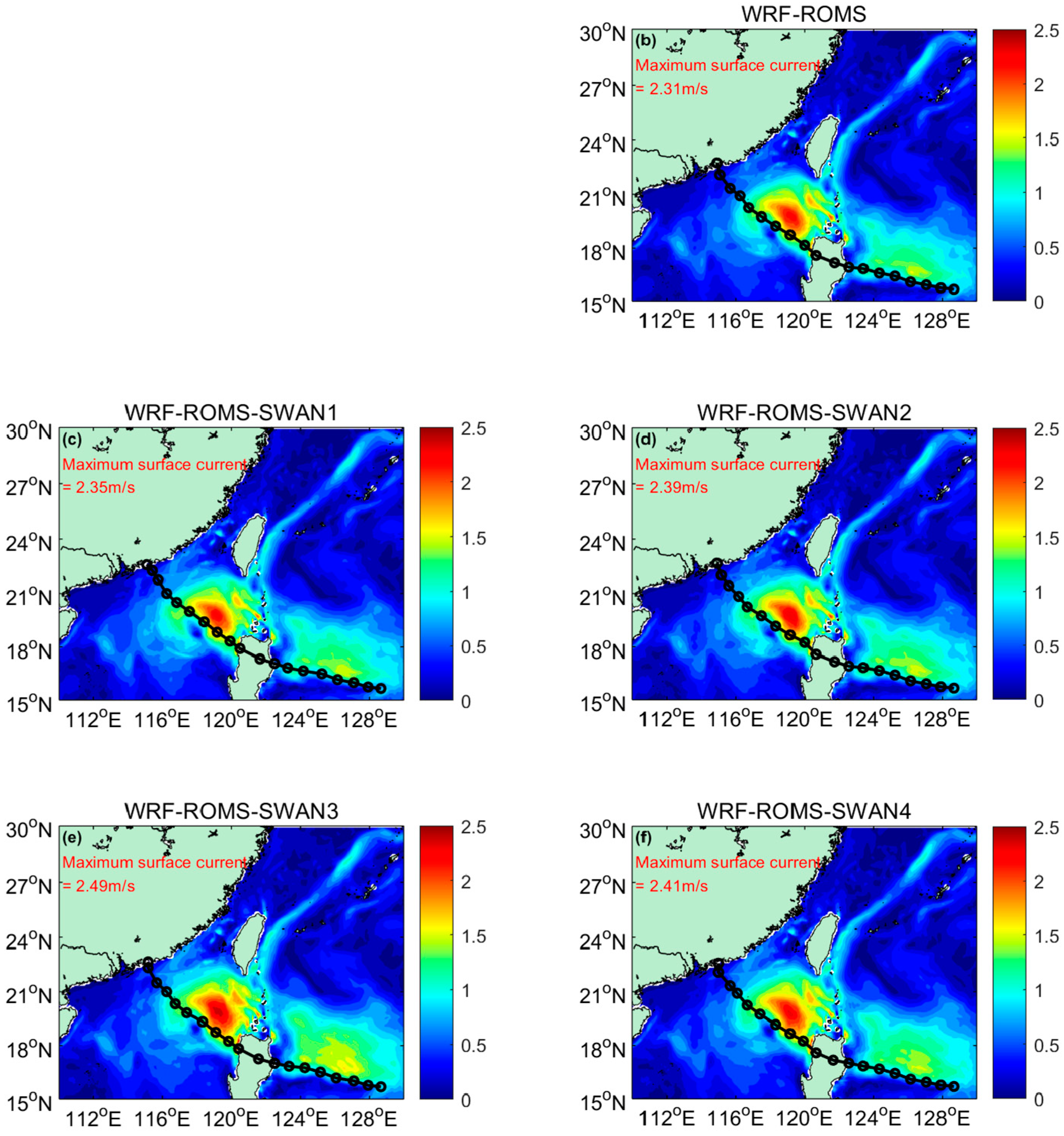
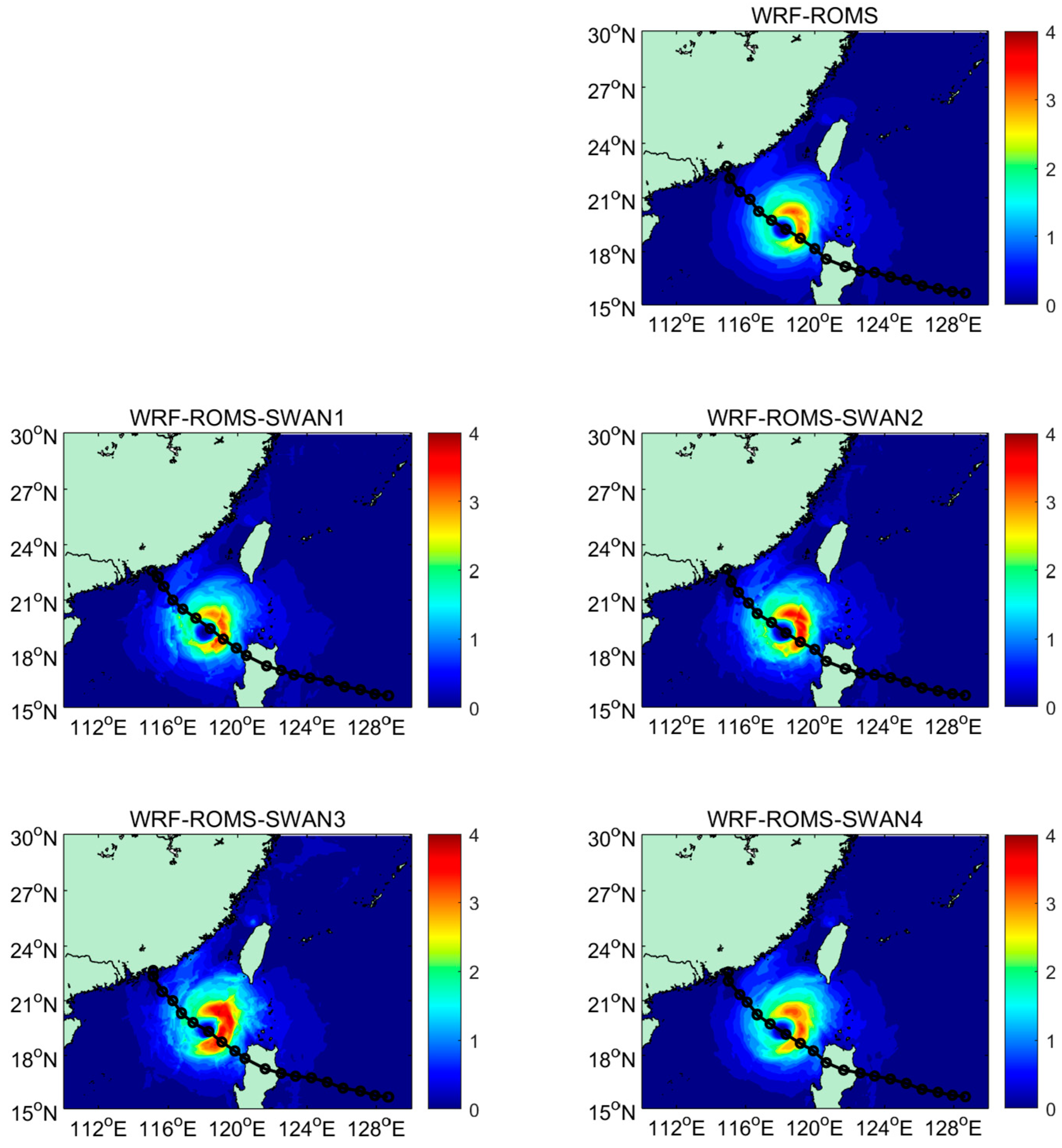
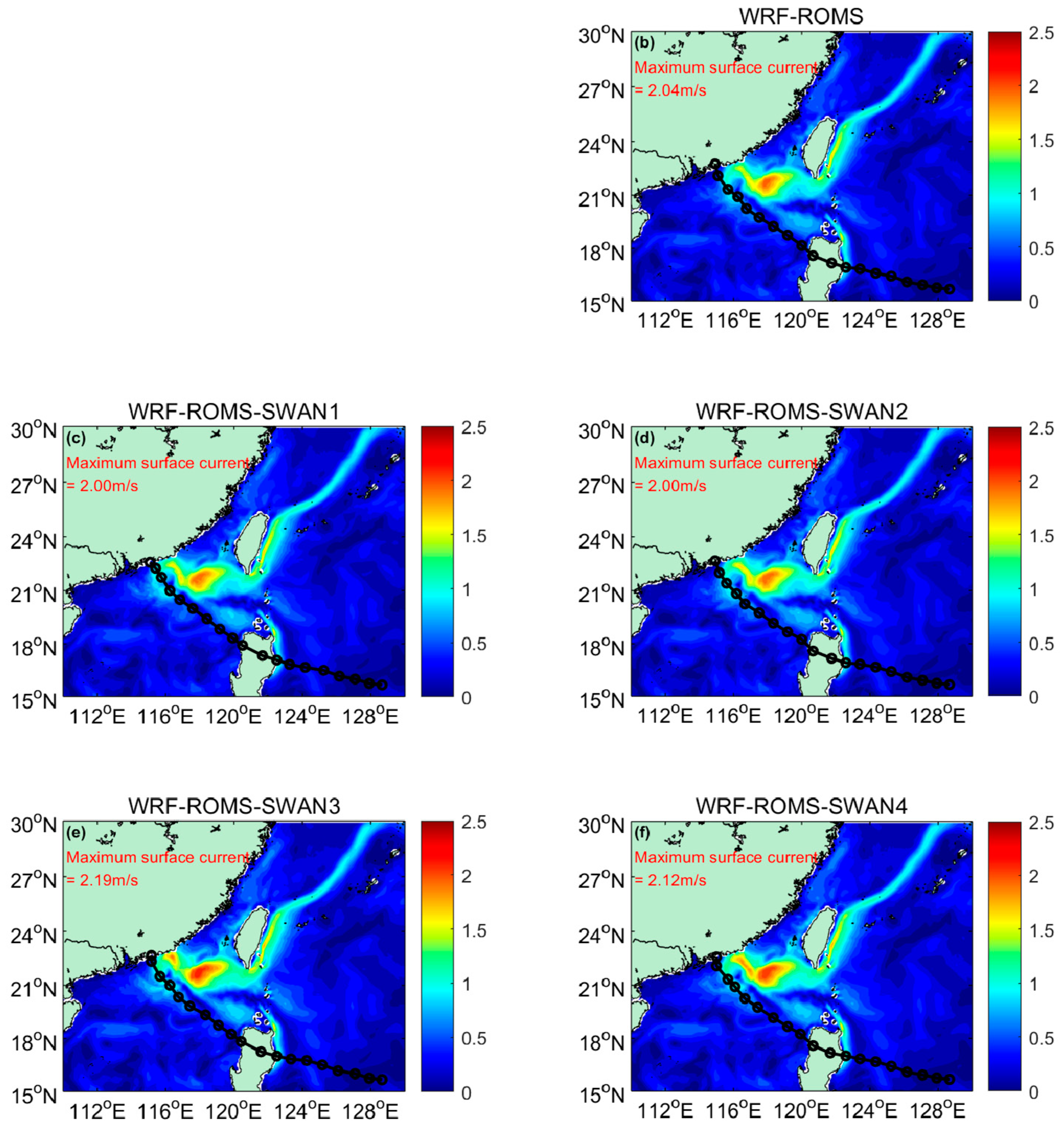
3.1. Surface Currents

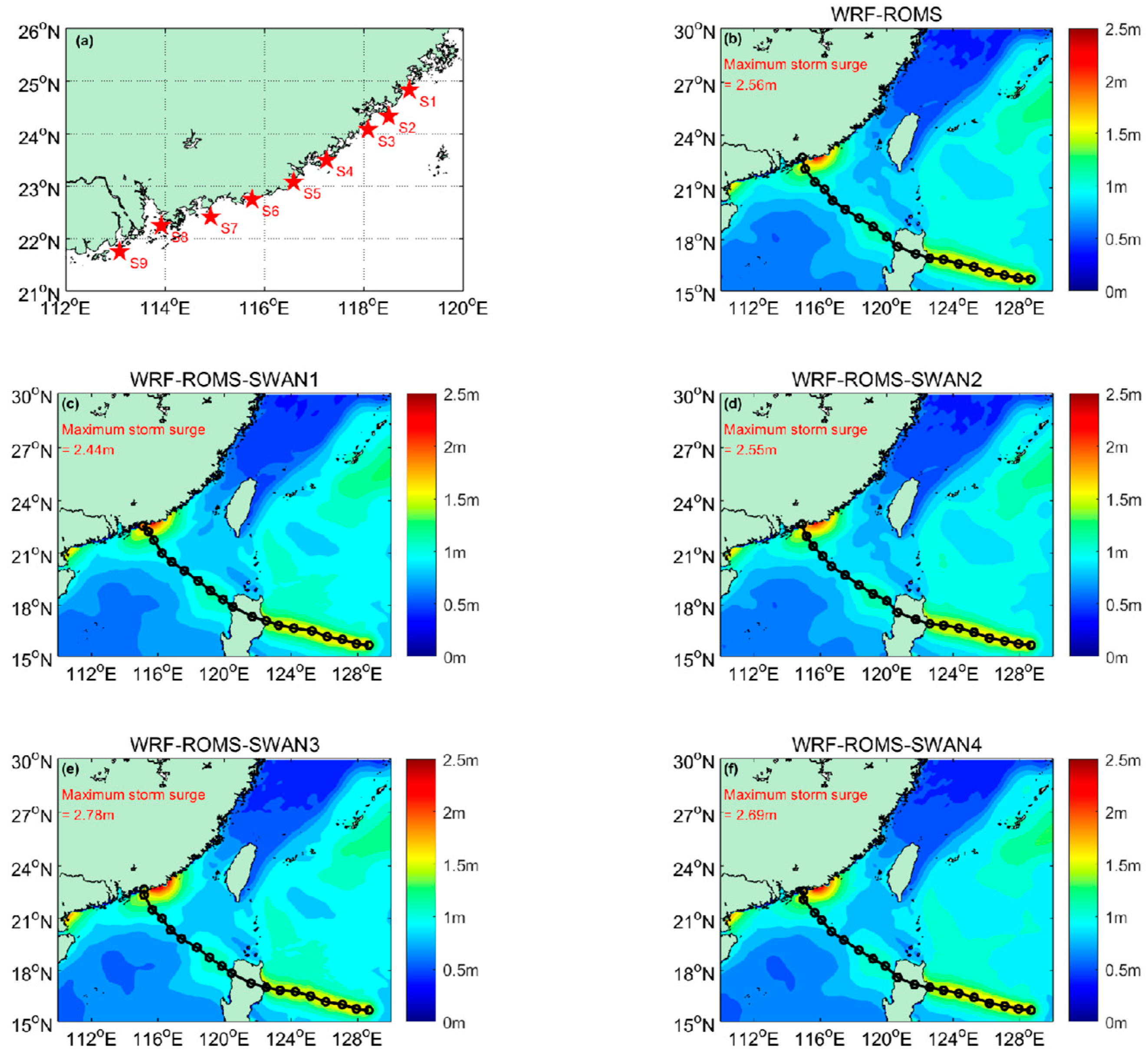
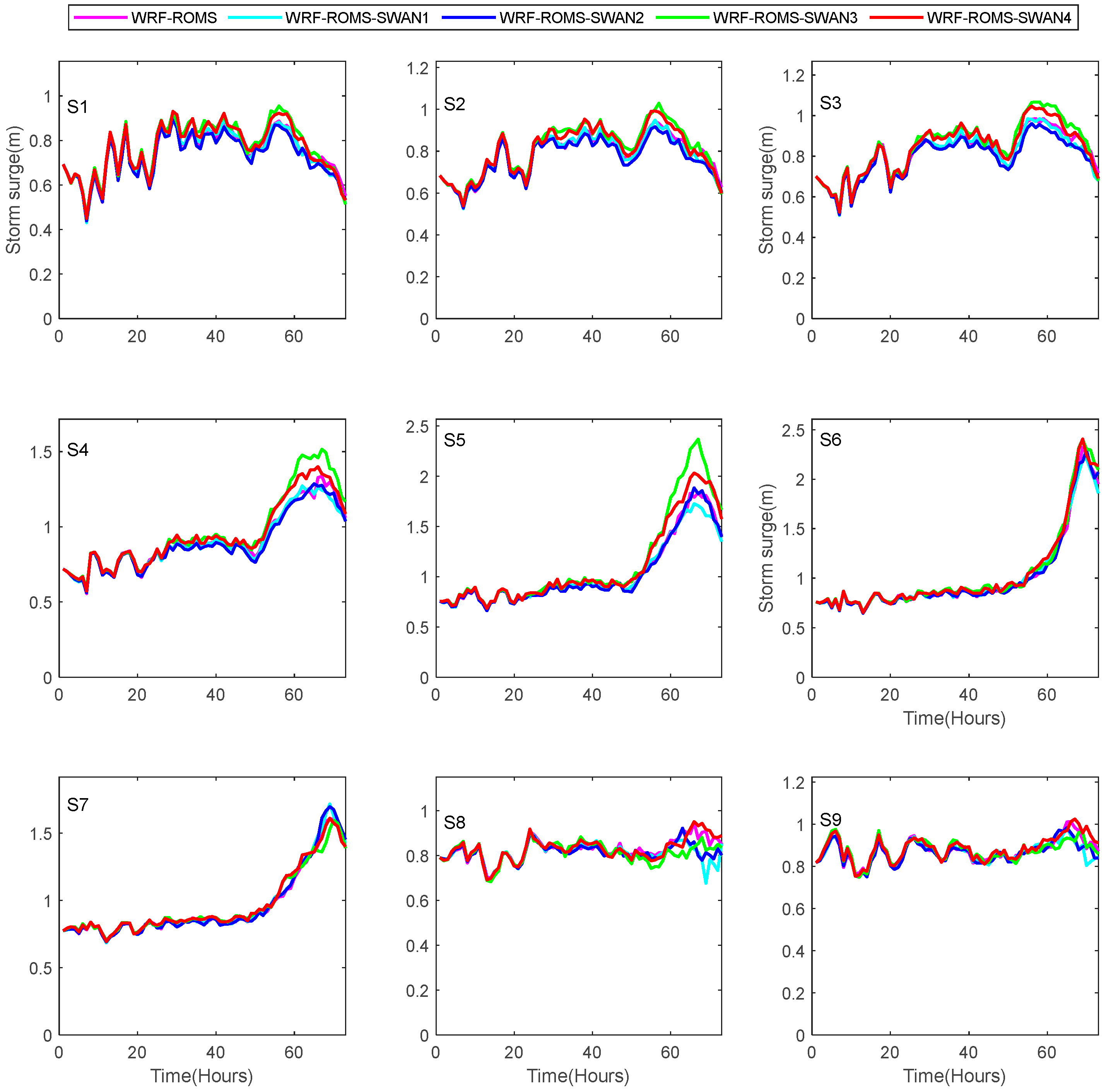
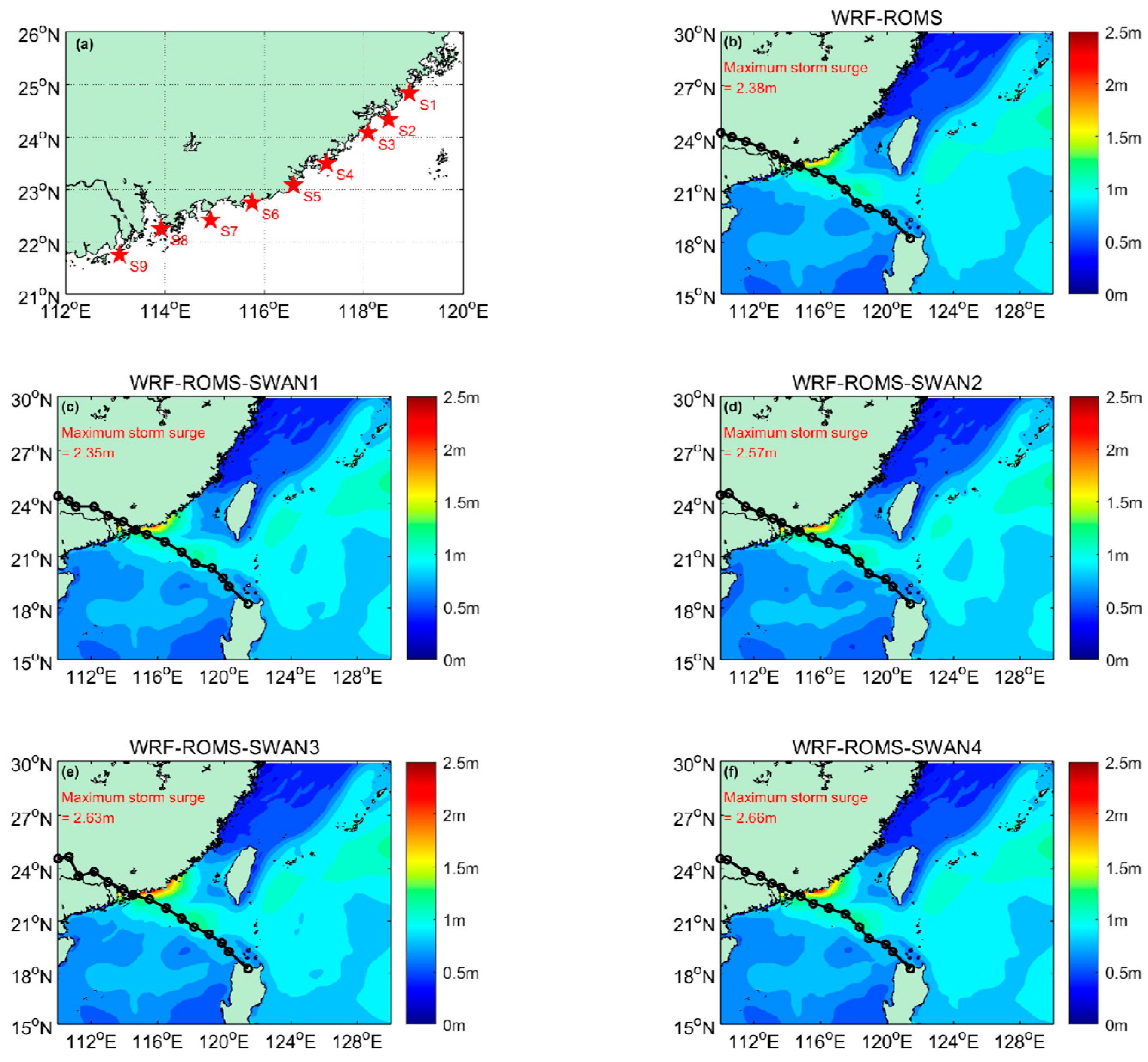
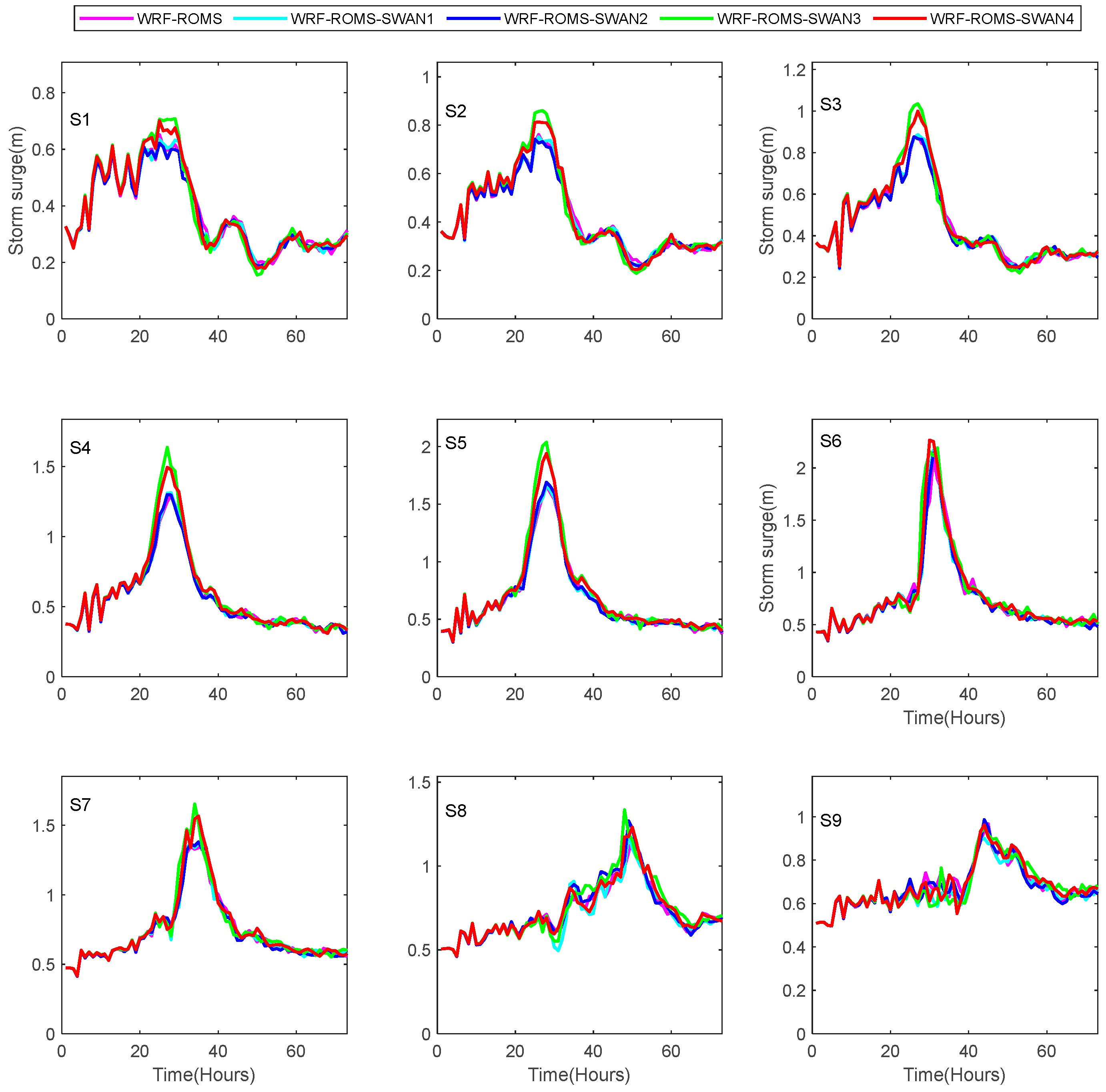
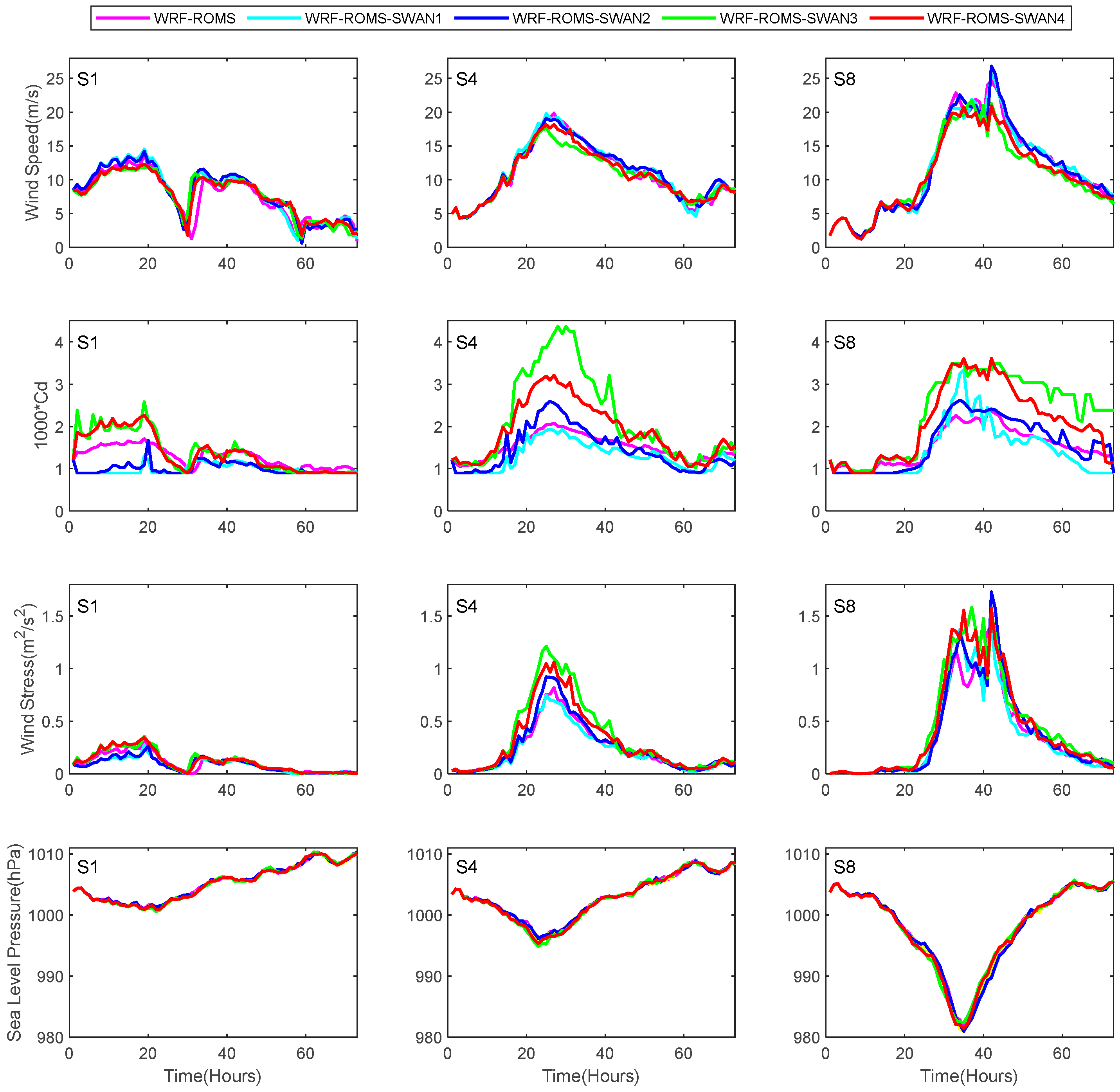
The parameterization of sea surface roughness plays a crucial role in modulating the momentum exchange between the atmosphere and the ocean, which, in turn, impacts the ocean’s dynamic processes, with surface currents being of particular significance. This section examines the simulated surface currents. When a typhoon is located over the open ocean, the sea surface currents near the radius of maximum wind speed are predominantly influenced by surface winds and exhibit minimal interaction with coastlines or tidal currents. The intense winds associated with a typhoon exert wind stress on the sea surface, facilitating the transfer of momentum from the atmosphere to the ocean and driving ocean surface currents [13]. Moreover, the low-pressure center of a typhoon generates a pressure gradient force that induces water to flow from regions of higher pressure (outside the typhoon) toward regions of lower pressure (inside the typhoon). Consequently, ocean surface currents converge toward the typhoon’s center, particularly in the vicinity of the maximum wind speed radius. This convergence can result in localized enhancements in surface current speeds.

To conduct the analysis, the simulation results of Typhoon Haima at the 51st hour were chosen. The corresponding simulated surface currents are presented in Figure 1, which provides a visual representation of the current patterns. Consistent with typhoon-induced current asymmetry, rightward track regions exhibited 15–20% higher surface current velocities compared to leftward sectors (Figure 1). This observation aligns with the asymmetric characteristics of typhoon-induced currents, where the right side of the typhoon’s path usually experiences stronger wind forcing, leading to enhanced surface currents.

When comparing the simulation results across different experiments, the maximum ocean surface currents simulated by each experiment were 2.31 m/s, 2.35 m/s, 2.39 m/s, 2.49 m/s, and 2.41 m/s, corresponding to the WRF-ROMS and WRF-ROMS-SWAN experiments 1 through 4, respectively. Although the maximum surface currents simulated by each group of experiments are quite similar, the WRF-ROMS-SWAN3 experiment demonstrates the broadest spatial influence, suggesting that this particular parameterization scheme may be more effective in capturing the extent of the surface currents. This could be attributed to a more accurate depiction of wind stress and its impact on the ocean surface.

Notably, the simulated wind speed in the WRF-ROMS-SWAN3 experiment is significantly weaker than that in the other experiments at the 51st hour of simulation (as shown in Figure 4 of the work of Ref. [11]. This raises an interesting point: despite the weaker wind speeds, the WRF-ROMS-SWAN3 experiment produces stronger surface currents. The inverse relationship between simulated wind speeds and surface current magnitudes in WRF-ROMS-SWAN3 reveals enhanced momentum transfer efficiency through its wave-state-dependent $C_d$ formulation.

To elucidate this phenomenon, the $C_d$ and sea surface wind stress at the corresponding time were also examined. The spatial distributions of $C_d$ in different experiments are illustrated in Figure 9 of the work of Ref. [11], where significant differences are observed. In the WRF-ROMS experiment, $C_d$ is mainly correlated with wind speed; hence, its spatial distributions are highly similar. In contrast, in the WRF-ROMS-SWAN experiments 1 to 4, the spatial distribution of $C_d$ is influenced not only by wind speed but also by the wave field. Notably, the $C_d$ value in the WRF-ROMS-SWAN3 experiment is significantly higher than that in the other experiments, which may contribute to its enhanced performance in simulating surface currents despite lower wind speeds.

Wind stress was computed using the wind speed and $C_d$ data according to Equation (1) during the simulation, and the wind stress distribution is illustrated in Figure 2. The results revealed that the wind stress in the WRF-ROMS-SWAN3 experiment was the highest among all experiments, attributed to its larger $C_d$ value, despite having a lower wind speed compared to the other experiments. This indicates that the greater sea surface roughness in the WRF-ROMS-SWAN3 experiment led to increased bottom stress in the atmospheric model, which subsequently weakened the wind field relative to the other experiments. However, the sea surface wind stress was also higher than in the other experiments, thereby driving stronger sea surface currents.

The comparison of surface currents in different experiments, along with the analysis of $C_d$ and sea surface wind stress, provides valuable insights into the performance and sensitivity of various air–sea coupled models. It highlights the importance of optimizing the parameterization schemes of $C_d$ and understanding the complex feedback mechanisms between the atmosphere and ocean. The results of this research provide valuable guidance for enhancing the operational marine forecasting system and promoting the development of more integrated models that are capable of predicting storm surges and sea level anomalies.

For Typhoon Nida, the intensity is not as strong as that of Typhoon Haima, and consequently, the surface currents caused by Typhoon Nida are also relatively smaller. However, the conclusion remains consistent: the results from the WRF-ROMS-SWAN3 experiment show the largest surface currents, with a maximum value of 2.19 m/s (Figure 3). We also analyzed the $C_d$ and wind stresss, which were found to be the largest in the WRF-ROMS-SWAN3 experiment as well (For brevity the figures are not shown here).

Although Typhoon Nida was less intense, the surface current and wave field characteristics it induced were similar to those of Typhoon Haima, particularly in terms of the higher flow velocity on the right side of the typhoon’s track. The WRF-ROMS-SWAN3 experiment demonstrated good performance in simulating the surface currents of both typhoons, indicating that the parameterization scheme used in this experiment is highly applicable across typhoons of different intensities. These findings help to improve and validate air–sea coupled models, enhancing the simulation and prediction capabilities for oceanic dynamic processes induced by typhoons.

3.2. Storm Surge

Another important ocean dynamic process during a typhoon is the storm surge, which can lead to significant economic losses and casualties. For instance, during Typhoon Haima, the storm surge disaster resulted in an economic loss of approximately USD 1.93 billion. The maximum storm surge observed occurred on the right flank of the typhoon’s landfall location. To elucidate the influence of different sea surface roughness parameterization schemes on the simulation of storm surges, Figure 4 presents the simulated maximum storm surges for various experiments. These simulations are crucial for understanding and predicting the potential damage of storm surges, which can affect a wide range of sectors, including agriculture, aquaculture, shipping, and infrastructure. Accurate simulations can help in developing more effective disaster prevention and mitigation strategies to reduce the economic and social impacts of such natural disasters.

As shown in Figure 4, the simulated maximum storm surge value differs among the experiments. In the WRF-ROMS-SWAN1 experiment, it reaches 2.44 m, while in the WRF-ROMS-SWAN3 experiment, it reaches 2.78 m. The significant storm surge predominantly occurred along the coastal regions situated to the right of the typhoon’s trajectory. This is attributed to the onshore wind direction in this region during the typhoon, which pushes seawater towards the coast, thereby increasing the sea level [35].

To provide a more detailed analysis of the storm surge processes, Figure 5 illustrates the storm surge time series recorded at nine strategically chosen stations during Typhoon Haima. These stations were selected based on their locations in the coastal regions where the storm surge impact was most significant, as shown in Figure 4a. Specifically, stations S1 to S5 are located on the right flank of the typhoon’s path, stations S6 and S7 are positioned near the typhoon center, and stations S8 and S9 are on the left flank of the typhoon.

Through a comparative analysis of the storm surge simulations from the five experiments (as shown in Figure 4 and Figure 5), it is apparent that at stations S1 to S5, the storm surge simulated by the WRF-ROMS-SWAN3 experiment is significantly higher than that from the other experiments. This difference is likely attributable to the influence of wind stress, which is a key factor in determining storm surge height. In contrast, the results from stations S6 and S7, which are located near the typhoon center, show relatively consistent storm surge magnitudes across all experiments. On the left side of the typhoon’s path, a process of storm surge reduction may occur, characterized by a decrease in sea level. This phenomenon is explained by the strong winds near the typhoon’s center, which push seawater in the direction of the typhoon’s movement, leading to a relative decrease in the sea level on the left side.

Figure 6 presents time series data of wind speed, $C_d$, wind stress, and sea level pressure to illustrate the differences in storm surge outcomes among various experiments. For clarity, the results are shown only for three representative stations. The figure indicates that the wind speed in the WRF-ROMS-SWAN3 experiment was generally lower compared to that of other experiments at these stations. However, the wind stress in WRF-ROMS-SWAN3 was higher, primarily due to the larger $C_d$ values in this experiment. This higher wind stress explains why the storm surge simulated by WRF-ROMS-SWAN3 was generally the highest during Typhoon Haima.

At station S8, the maximum simulated storm surge in the WRF-ROMS-SWAN3 experiment was lower than in other experiments. This is attributed to the station’s location on the left side of the typhoon track and its proximity to the landfall point. Here, the impact of sea level pressure on the storm surge is substantial, overshadowing the influence of wind stress. Specifically, the sea level pressure can counteract the wind stress, resulting in a decrease in storm surge height.

These results highlight the necessity of incorporating both wind stress and sea level pressure into storm surge modeling, particularly in regions near the typhoon’s landfall point. The precise depiction of these factors is essential for enhancing the accuracy of storm surge predictions, thereby supporting more effective disaster preparedness and mitigation efforts.

For Typhoon Nida, the simulation results from different models exhibit some discrepancies. The WRF-ROMS-SWAN1 model simulates a maximum storm surge of 2.35 m, whereas the WRF-ROMS-SWAN4 model simulates a maximum storm surge of 2.66 m (as shown in Figure 7). These differences may be associated with various factors, including model configuration, parameterization methods, and initial and boundary conditions. For example, under different coupling modes, the models have different accuracies in simulating the path and intensity of the typhoon, which, in turn, affects the simulation results of the storm surge. Overall, a difference of 0.31 m is relatively significant in the simulation of storm surges, indicating that different model configurations have a fairly noticeable impact on the simulation results. Additionally, since the maximum wind speed of Typhoon Nida is higher than that of Typhoon Haima, the resulting maximum storm surge is also larger. We used the same nine stations to analyze the specific storm process. From the specific storm surge process (Figure 8), the conclusion is consistent with Haima; that is, for S1–S5 stations, the maximum storm surge simulated by WRF-ROMS-SWAN3 is the largest.

We also presented the charts of wind speed, $C_d$, wind stress, and sea surface pressure for three stations (S1, S4, and S8) during Typhoon Nida (Figure 9). It is evident that, for most of the time at these stations, the wind speed in the WRF-ROMS-SWAN3 experiment is the lowest compared to other experiments. However, due to the higher $C_d$ values in WRF-ROMS-SWAN3, the wind stress in this experiment is greater than that in the other experiments. This is why the storm surge of WRF-ROMS-SWAN3 is the largest for most of the time. However, the wind speed, $C_d$, and wind stress of WRF-ROMS-SWAN4 are quite similar to those of WRF-ROMS-SWAN3, and at times, they even surpass the results of WRF-ROMS-SWAN3. This leads to WRF-ROMS-SWAN4 simulating the largest storm surge. At station S8, the sea surface pressure is notably lower than at stations S1 and S4, and this has a significant impact. Therefore, the simulation results from all experimental groups at station S8 are relatively consistent.

4. Discussion

The WRF-ROMS-SWAN3 experiment shows excellent performance in simulating surface currents and storm surges. This can be mainly ascribed to its distinctive way of representing the wind stress drag coefficient ($C_d$), which is closely related to wave dynamics. The coupling between them plays a crucial role in enhancing the simulation accuracy. In traditional parameterizations (e.g., WRF-ROMS), $C_d$ is primarily governed by wind speed, leading to a simplified linear relationship that fails to capture the saturation of momentum transfer under high-wind conditions [29]. In contrast, the WRF-ROMS-SWAN3 experiment incorporates wave-state dependencies, where $C_d$ is modulated by both wind speed and wave age. This dual dependency enhances the realism of sea surface roughness calculations, as waves with longer fetch or higher steepness increase surface roughness [20], thereby amplifying wind stress even under lower wind speeds. This mechanism explains why WRF-ROMS-SWAN3 generated stronger surface currents despite weaker simulated winds (Figure 6): the elevated $C_d$ compensated for reduced wind momentum by enhancing the efficiency of energy transfer from the atmosphere to the ocean.

The asymmetry in surface current intensity (stronger currents on the typhoon’s right flank) further highlights the role of wave–current interactions. During typhoon passage, wind–wave alignment on the right side generates younger, steeper waves, which increase local roughness and $C_d$ [17]. These transient wave states intensify wind stress in specific regions, driving stronger convergence of surface currents toward the typhoon center. Conversely, on the left flank, wave decoupling from wind direction reduces roughness, leading to weaker stress and current velocities. This spatial heterogeneity underscores the necessity of integrating wave dynamics into coupled models to resolve momentum transfer gradients.

For storm surges, the dominance of wind stress over sea level pressure at coastal stations (S1–S5) arises from the combined effects of onshore winds and wave setup. The WRF-ROMS-SWAN3 experiment’s higher $C_d$ amplified wind stress, which directly enhanced water mass transport toward the coast. However, near the typhoon center (stations S6 and S7), the balance between wind stress and pressure gradient forces minimized inter-experiment differences. Here, the low-pressure-induced suction effect dominated surge dynamics, masking variations caused by $C_d$ parameterizations. This dichotomy illustrates how localized feedback mechanisms—wind stress in shallow coastal zones versus pressure gradients in deep offshore regions—govern surge magnitude.

The discrepancies between Typhoons Haima and Nida further emphasize environmental dependencies. Nida’s higher maximum wind speeds likely induced stronger wave breaking and sea spray, which nonlinearly modulate $C_d$ [28]. In such conditions, parameterizations that neglect spray-mediated momentum dissipation (e.g., WRF-ROMS-SWAN1) overestimate $C_d$, whereas schemes accounting for spray effects (e.g., WRF-ROMS-SWAN3) better replicate the observed saturation of drag coefficients [12]. This explains why WRF-ROMS-SWAN3 maintained accuracy across both typhoons, despite differences in intensity.

Ultimately, the sensitivity of simulations to $C_d$ parameterizations stems from the interplay between atmospheric forcing, wave-state variability, and ocean response. Models that decouple these components (e.g., WRF-ROMS) oversimplify momentum transfer pathways, while coupled frameworks (e.g., WRF-ROMS-SWAN) resolve critical feedback loops. Future efforts should prioritize dynamic $C_d$ schemes that adapt to real-time wave and spray conditions, particularly in coastal zones where surge predictions hinge on precise wind stress estimates.

5. Conclusions

The research results highlight the significant influence of air–sea momentum flux parameterization, especially the representation of the wind stress drag coefficient ($C_d$), on the accuracy of coupled atmosphere–wave–ocean models when simulating typhoon-induced surface currents and storm surges. The superior performance of the WRF-ROMS-SWAN3 experiment stems from its explicit incorporation of wave-state dependencies into $C_d$, which dynamically accounts for wavelength and wave age. This approach enhances sea surface roughness calculations, enabling more efficient momentum transfer from the atmosphere to the ocean, even under high-wind conditions where traditional wind-speed-dependent schemes (e.g., WRF-ROMS) fail to capture saturation effects. The resultant amplification of wind stress compensates for weaker simulated winds, driving stronger surface currents and elevated storm surges in coastal regions.

The spatial asymmetry in surface currents—stronger flows on the typhoon’s right flank—is mechanistically linked to wave–current interactions. Younger, steeper waves on the right side increase local roughness, intensifying wind stress and current convergence toward the typhoon center. Conversely, reduced coupling between wind and waves on the left flank diminishes stress and flow velocities. For storm surges, wind stress dominates in shallow coastal zones (e.g., stations S1–S5), where elevated $C_d$ enhances onshore water transport, while pressure gradients prevail near the typhoon center (e.g., stations S6 and S7), minimizing parameterization-induced discrepancies.

The variation in model performance across typhoons (Haima vs. Nida) underscores the environmental sensitivity of $C_d$. Under extreme winds (e.g., Typhoon Nida), schemes neglecting sea-spray-mediated momentum dissipation (e.g., WRF-ROMS-SWAN1) overestimate drag, whereas wave-coupled frameworks (e.g., WRF-ROMS-SWAN3) better replicate observed saturation trends. This highlights the necessity of adaptive $C_d$ parameterizations that integrate real-time wave and spray dynamics, particularly for high-intensity typhoons.

To advance operational marine forecasting, future efforts should prioritize the development of dynamically coupled models that resolve atmosphere–wave–ocean feedbacks, with a focus on coastal regions where surge prediction accuracy hinges on precise wind stress estimates. Additionally, expanding validation datasets to include diverse typhoon intensities and oceanic conditions will further refine parameterization schemes, ultimately enhancing the reliability of storm surge and surface current forecasts.

References

1. Bhattacharya, T.; Chakraborty, K.; Anthoor, S.; Ghoshal, P.K. An assessment of air-sea CO2 flux parameterizations during tropical cyclones in the Bay of Bengal. Dyn. Atmos. Oceans 2023, 103, 101390. [Google Scholar] [CrossRef]
2. Gröger, M.; Dieterich, C.; Haapala, J.; Ho-Hagemann, H.T.M.; Hagemann, S.; Jakacki, J.; May, W.; Meier, H.E.M.; Miller, P.A.; Rutgersson, A.; et al. Coupled regional earth system modeling in the Baltic Sea region. Earth Syst. Dynam. 2021, 12, 939–973. [Google Scholar] [CrossRef]
3. Wahle, K.; Staneva, J.; Koch, W.; Fenoglio-Marc, L.; Ho-Hagemann, H.T.M.; Stanev, E.V. An atmosphere–wave regional coupled model: Improving predictions of wave heights and surface winds in the southern north Sea. Ocean Sci. 2017, 13, 289–301. [Google Scholar] [CrossRef]
4. Wiese, A.; Stanev, E.; Koch, W.; Behrens, A.; Geyer, B.; Staneva, J. The impact of the two-way coupling between wind wave and atmospheric models on the lower atmosphere over the north Sea. Atmosphere 2019, 10, 386. [Google Scholar] [CrossRef]
5. Wiese, A.; Staneva, J.; Ho-Hagemann, H.T.M.; Grayek, S.; Koch, W.; Schrum, C. Internal model variability of ensemble simulations with a regional coupled wave-atmosphere model GCOAST. Front. Mar. Sci. 2020, 7, 596843. [Google Scholar] [CrossRef]
6. Varlas, G.; Spyrou, C.; Papadopoulos, A.; Korres, G.; Katsafados, P. One-year assessment of the CHAOS two-way coupled atmosphere-ocean wave modelling system over the Mediterranean and black seas. Mediterr. Mar. Sci. 2020, 21, 372–385. [Google Scholar] [CrossRef]
7. Breivik, Ø.; Mogensen, K.; Bidlot, J.R.; Balmaseda, M.A.; Janssen, P.A.E.M. Surface wave effects in the NEMO ocean model: Forced and coupled experiments. J. Geophys. Res. Oceans 2015, 120, 2973–2992. [Google Scholar] [CrossRef]
8. Alari, V.; Staneva, J.; Breivik, Ø.; Bidlot, J.R.; Mogensen, K.; Janssen, P. Surface wave effects on water temperature in the Baltic Sea: Simulations with the coupled NEMO-WAM model. Ocean Dyn. 2016, 66, 917–930. [Google Scholar] [CrossRef]
9. Wu, L.; Sahlée, E.; Nilsson, E.; Rutgersson, A. A review of surface swell waves and their role in air–sea interactions. Ocean Modell. 2024, 190, 102397. [Google Scholar] [CrossRef]
10. Fan, Y.; Ginis, I.; Hara, T. Momentum flux budget across the air–sea interface under uniform and tropical cyclone winds. J. Phys. Oceanogr. 2010, 40, 2221–2242. [Google Scholar] [CrossRef]
11. Feng, X.; Sun, J.; Yang, D.; Yin, B.; Gao, G.; Wan, W. Effect of drag coefficient parameterizations on air–sea coupled simulations: A case study for Typhoons Haima and Nida in 2016. J. Atmos. Oceanic Technol. 2021, 38, 977–993. [Google Scholar] [CrossRef]
12. Liu, B.; Guan, C.; Xie, L. The wave state and sea spray related parameterization of wind stress applicable from low to extreme winds. J. Geophys. Res. 2012, 117, C00J22. [Google Scholar] [CrossRef]
13. Fairall, C.W.; Bradley, E.F.; Hare, J.E.; Grachev, A.A.; Edson, J.B. Bulk parameterization of air-sea fluxes for tropical ocean-global atmosphere coupled-ocean-atmosphere response experiment. J. Geophys. Res. Oceans 1996, 101, 3747–3764. [Google Scholar] [CrossRef]
14. Grachev, A.A.; Fairall, C.W.; Larsen, S.E. On the determination of the neutral drag coefficient in the convective boundary layer. Bound.-Layer Meteorol. 1998, 86, 257–278. [Google Scholar] [CrossRef]
15. Stewart, R.W. The air-sea momentum exchange. Bound.-Layer Meteorol. 1974, 6, 151–167. [Google Scholar] [CrossRef]
16. Toba, Y.; Iida, N.; Kawamura, H.; Ebuchi, N.; Jones, I.S.F. Wave dependence of sea-surface wind stress. J. Phys. Oceanogr. 1990, 20, 705–721. [Google Scholar] [CrossRef]
17. Oost, W.A.; Komen, G.J.; Jacobs, C.M.J.; Van Oort, C. New evidence for a relation between wind stress and wave age from measurements during ASGAMAGE. Bound.-Layer Meteorol. 2002, 103, 409–438. [Google Scholar] [CrossRef]
18. Drennan, W.M.; Taylor, P.K.; Yelland, M.J. Parameterizing the sea surface roughness. J. Phys. Oceanogr. 2005, 35, 835–848. [Google Scholar] [CrossRef]
19. Anctil, F.; Donelan, M.A. Air-water momentum flux observations over shoaling waves. J. Phys. Oceanogr. 1996, 26, 1344–1353. [Google Scholar] [CrossRef]
20. Taylor, P.K.; Yelland, M.J. The dependence of sea surface roughness on the height and steepness of the waves. J. Phys. Oceanogr. 2001, 31, 572–590. [Google Scholar] [CrossRef]
21. Guan, C.; Xie, L. On the linear parameterization of drag coefficient over sea surface. J. Phys. Oceanogr. 2004, 34, 2847–2851. [Google Scholar] [CrossRef]
22. Smith, S.D.; Anderson, R.J.; Oost, W.A.; Kraan, C.; Maat, N.; De Cosmo, J. Sea surface wind stress and drag coefficients: The HEXOS results. Bound.-Layer Meteorol. 1992, 60, 109–142. [Google Scholar] [CrossRef]
23. Johnson, H.K.; Højstrup, J.; Vested, H.J.; Larsen, S.E. On the dependence of sea surface roughness on wind waves. J. Phys. Oceanogr. 1998, 28, 1702–1716. [Google Scholar] [CrossRef]
24. Drennan, W.M.; Graber, H.C.; Hauser, D.; Quentin, C. On the wave age dependence of wind stress over pure wind seas. J. Geophys. Res. 2003, 108, 8062. [Google Scholar] [CrossRef]
25. Gao, Z.; Wang, Q.; Wang, S. An alternative approach to sea surface aerodynamic roughness. J. Geophys. Res. 2006, 111, D22108. [Google Scholar] [CrossRef]
26. Hu, Y.; Shao, W.; Wang, X.; Zuo, J.; Jiang, X. Analysis of wave breaking on synthetic aperture radar at C-band during tropical cyclones. Geo-Spat. Inf. Sci. 2024, 27, 2109–2122. [Google Scholar] [CrossRef]
27. Alamaro, M. Wind Wave Tank for Experimental Investigation of Momentum and Enthalpy Transfer from the Ocean Surface at High Wind Speed. Master’s Thesis, Massachusetts Institute of Technology, Cambridge, MA, USA, 2001. [Google Scholar]
28. Alamaro, M.; Emanuel, K.; Colton, J.; McGillis, W.; Edson, J. Experimental investigation of air–sea transfer of momentum and enthalpy at high wind speed. In Proceedings of the 25th Conference on Hurricanes and Tropical Meteorology, San Diego, CA, USA, 29 April–3 May 2002; pp. 667–668. [Google Scholar]
29. Powell, M.D.; Vickery, P.J.; Reinhold, T.A. Reduced drag coefficient for high wind speeds in tropical cyclones. Nature 2003, 422, 279–283. [Google Scholar] [CrossRef]
30. Lin, S.; Sheng, J. Revisiting dependences of the drag coefficient at the sea surface on wind speed and sea state. Cont. Shelf Res. 2020, 207, 104188. [Google Scholar] [CrossRef]
31. Businger, J.A.; Wyngaard, J.C.; Izumi, Y.; Bradley, E.F. Flux-profile relationships in the atmospheric boundary layer. J. Atmos. Sci. 1971, 28, 181–189. [Google Scholar] [CrossRef]
32. Skamarock, W.C.; Klemp, J.B.; Dudhia, J.; Gill, D.O.; Barker, D.M.; Wang, W.; Powers, J.G. A Description of the Advanced Research WRF Version 2; National Center for Atmospheric Research: Boulder, CO, USA, 2005; p. 88. [Google Scholar] [CrossRef]
33. Warner, J.C.; Sherwood, C.R.; Signell, R.P.; Harris, C.K.; Arango, H.G. Development of a three-dimensional, regional, coupled wave, current, and sediment-transport model. Comput. Geosci. 2008, 34, 1284–1306. [Google Scholar] [CrossRef]
34. Warner, J.C.; Armstrong, B.; He, R.; Zambon, J.B. Development of a Coupled Ocean–Atmosphere–Wave–Sediment Transport (COAWST) modeling system. Ocean Modell. 2010, 35, 230–244. [Google Scholar] [CrossRef]
35. Leung, N.-C.; Chow, C.-K.; Lau, D.-S.; Lam, C.-C.; Chan, P.-W. WRF-ROMS-SWAN Coupled Model Simulation Study: Effect of Atmosphere–Ocean Coupling on Sea Level Predictions Under Tropical Cyclone and Northeast Monsoon Conditions in Hong Kong. Atmosphere 2024, 15, 1242. [Google Scholar] [CrossRef]
Figure 1. Surface currents at the time of 51st hour of the simulation for Typhoon Haima. The values of the simulated maximum surface current velocity for the different numerical experiments are also shown in the corresponding subplot.
Jmse 13 00541 g001
Figure 2. Sea surface wind stress at the time of 51st hour of the simulation for Typhoon Haima.
Jmse 13 00541 g002
Figure 3. Surface currents at the time of 27th hour of the simulation for Typhoon Nida.
Jmse 13 00541 g003
Figure 4. Simulated maximum storm surge distribution during Typhoon Haima for five numerical experiments (af). The red stars represent the nine stations selected for analyzing the storm surge time series.
Jmse 13 00541 g004
Figure 5. Storm surge time series during Typhoon Haima at coastal stations; see Figure 4a for station locations.
Jmse 13 00541 g005
Figure 6. Time series of wind speed, C d , wind stress and sea level pressure at stations S1, S4 and S8 along the coast during typhoon Haima.
Jmse 13 00541 g006
Figure 7. Simulated maximum storm surge distribution during Typhoon Nida for five numerical experiments (af). The red stars represent the nine stations selected for analyzing the storm surge time series.
Jmse 13 00541 g007
Figure 8. Storm surge time series during Typhoon Nida at coastal stations; see Figure 7a for station locations.
Jmse 13 00541 g008
Figure 9. Time series of wind speed, C d , wind stress and sea level pressure at stations S1, S4 and S8 along the coast during typhoon Nida.
Jmse 13 00541 g009
Disclaimer/Publisher’s Note: The statements, opinions and data contained in all publications are solely those of the individual author(s) and contributor(s) and not of MDPI and/or the editor(s). MDPI and/or the editor(s) disclaim responsibility for any injury to people or property resulting from any ideas, methods, instructions or products referred to in the content.