Improved Variational Mode Decomposition in Pipeline Leakage Detection at the Oil Gas Chemical Terminals Based on Distributed Optical Fiber Acoustic Sensing System

Abstract

Leakage in oil and gas transportation pipelines is a critical issue that often leads to severe hazardous accidents at oil and gas chemical terminals, resulting in devastating consequences such as ocean environmental pollution, significant property damage, and personal injuries. To mitigate these risks, timely detection and precise localization of pipeline leaks are of paramount importance. This paper employs a distributed fiber optic sensing system to collect pipeline leakage signals and processes these signals using the traditional variational mode decomposition (VMD) algorithm. While traditional VMD methods require manual parameter setting, which can lead to suboptimal decomposition results if parameters are incorrectly chosen, our proposed method introduces an improved particle swarm optimization algorithm to automatically determine the optimal parameters. Furthermore, we integrate VMD with fuzzy dispersion entropy to effectively select and reconstruct intrinsic mode functions, significantly enhancing the denoising performance. Our results demonstrate that this approach can achieve a signal-to-noise ratio of up to 24.15 dB and reduce the mean square error to as low as 0.0027, showcasing its superior capability in noise reduction. Additionally, this paper proposes a novel threshold setting technique that addresses the limitations of traditional methods, which often rely on instantaneous values and are prone to false alarms. This innovative approach significantly reduces the false alarm rate in gas pipeline leakage detection, ensuring higher detection accuracy and reliability. The proposed method not only advances the technical capabilities of pipeline leakage monitoring but also offers strong practical applicability, making it a valuable tool for enhancing the safety and efficiency of oil and gas transportation systems.

1. Introduction

Pipeline transportation is widely employed for the conveyance of critical chemical raw materials, such as oil and natural gas, owing to its high efficiency, safety, and cost-effectiveness. In maritime environments, oil and gas chemical terminals play a crucial role as key hubs for the transportation and storage of these resources, serving as fundamental nodes within the maritime transportation network. Since oil and gas must temporarily halt at these terminals during transit and transfer, pipeline leakage at these sites is a major contributor to significant hazardous maritime incidents. Consequently, ensuring the safety of storage and transportation pipelines in the maritime settings is of critical importance for the overall security of oil and gas chemical terminals.

Non-destructive testing methods have increasingly gained prominence in pipeline leak detection due to their effectiveness and versatility. The most prominent techniques include pressure waves monitoring [1], ultrasound spectroscopy [2], time-domain and frequency-domain reflectometry [3], elastic waves [4], and signals from acoustic or vibration sensors detect [5,6]. Wang et al. [7] developed a fiber Bragg grating pipe-fixture sensor array to detect pipeline leakage and measure the pressure variations in the NPW signals. Muhammad et al. [8] introduced a deep learning-based pipeline leak detection algorithm that uses acoustic emission signals with great accuracy. Zahoor et al. [9] proposed a novel multiscale Mann–Whitney test applied to acoustic emission hit features to derive a new vulnerability index feature. Xiao et al. [10] conducted an experimental investigation into the feasibility of vibro-acoustic techniques for leak detection and localization in buried large-diameter gas pipelines. While these methods have demonstrated effectiveness in post-leakage scenarios, they are not without limitations, including challenges in precise positioning, restricted detection ranges, high operational costs, and a lack of early warning capabilities. Furthermore, the bustling activity of ships entering and exiting dock areas complicates routine radiographic testing, often necessitating isolation and making coordination difficult. Additionally, some crude oil or fuel oil pipelines s suffer from severe internal wall deposits and liquid accumulation, leading to insufficient exposure or even complete penetration failure in radiographic test results.

The emergence of novel sensing technologies utilizing optical fibers as both sensing elements and light transmission media has effectively addressed the limitations of traditional methods, providing innovative solutions for pipeline leakage detection [11]. The oil and gas chemical industry, characterized by high risk, strong corrosiveness, and flammability, presents significant challenges for the deployment of electrical sensors, particularly in hazardous environments such as oil and gas injection sites and wells. Distributed optical fiber acoustic sensing system (DAS), a cutting-edge technology in the field of distributed optical fiber monitoring, demonstrate exceptional resistance to electromagnetic and radio frequency interference, flexible deployment capabilities, and extensive monitoring range. These systems facilitate both distributed and network measurements [12,13]. Notably, the absence of electrical signals in DAS sensing components ensures excellent explosion-proof performance, making them particularly suitable for monitoring pipeline leaks in the flammable and explosive environments of the oil and gas chemical industry. Pavol Stajanca et al. [14] employed a DAS system to monitor gas pipeline leaks by directly winding optical fibers around the pipe wall to detect vibrations caused by leaks. However, the experimental results were notably affected by external factors, resulting in low positioning accuracy and requiring a substantial amount of optical fiber.

In contrast to conventional DAS-based leak detection methodologies, Wu et al. [15] installed the fiber-optic cable on the outside surface of the water pipe and introduced a leak identification algorithm utilizing 3D-convolutional neural networks. In this paper, DAS is used for pipeline monitoring signal acquisition. The detection fiber in this system is a single-mode compact type, and the sensing fiber is suspended in a relaxed state on the side of the pipeline. An acoustic sensor is positioned in a circular structure near the pipeline leakage hole to detect the sound of pipeline leakage.

For advanced processing of DAS-acquired pipeline signals, adaptive signal analysis methods are commonly used, such as empirical mode decomposition (EMD) algorithm, variational mode decomposition (VMD) algorithm, etc. However, EMD can suffer from mode aliasing [16,17], which limits its applicability. In contrast, the VMD algorithm [18] can effectively mitigate the drawbacks associated with EMD. Despite its advantages, the traditional VMD method still has some limitations in practical applications, requiring manual setting of key parameters such as mode number K and penalty factor α. For example, when dealing with leakage signals, if the mode number K is set improperly, it may lead to mode aliasing or incomplete decomposition, making it difficult to accurately extract fault features [19]. Therefore, selecting the appropriate parameter combination [K, α] is essential for achieving the desired decomposition effect of VMD algorithm.

The development of swarm intelligence optimization algorithms has significantly advanced their application in optimizing VMD parameters, leading to enhanced signal processing outcomes. Peng et al. [20] proposed a pipeline leak localization method based on VMD sparrow search algorithm (SSA) optimization and generalized quadratic cross-correlation. This approach leverages sample entropy and employs SSA optimization to refine the two key parameters of VMD. The experiment shows that the minimum relative error of this method can reach 0.6%. Du et al. [21] proposed an algorithm based on the Halton sequence and the Laplace crossover operator within the sparrow search algorithm–VMD framework to select the optimal VMD parameters. However, this approach only optimized the parameter α and did not address the parameter K. Jiang et al. [22]. proposed a denoising method based on VMD technology, utilizing information entropy to optimize the parameter K and ignore the parameter α. Diao et al. [23] developed a particle swarm optimization (PSO) algorithm that enhances the maximum entropy of intrinsic mode functions (IMFs) [18], and applied this improved algorithm to optimize both VMD parameters K and α. Nevertheless, traditional PSO algorithms often face challenges, such as convergence to local optima, limiting their effectiveness in complex optimization tasks.

In response to the existing problems, this work makes the following contributions:

• To combine particle swarm optimization with VMD and propose an improved particle swarm optimization (IPSO) algorithm for the first time, which optimizes the decomposition mode number K and penalty factor α.
• To employ a denoising method combining VMD and fuzzy dispersion entropy is first proposed to determine the effective IMFs.
• To present a new threshold setting method, which can avoid the drawbacks of traditional methods that rely on instantaneous values to determine leaks.

The subsequent sections of this article are organized as follows: Section 2 introduces the proposed methodology. Section 3 presents the leakage detection method based on IPSO–VMD, developed from the aforementioned methodology. Section 4 discusses the experimental results and provides a comprehensive discussion. Finally, Section 5 offers a conclusion.

2. Methodology

2.1. Brief Description of VMD

VMD is an adaptive, non-recursive method that decomposes signals into a finite sum of IMF components. This method is particularly well suited for the analysis and processing of nonlinear and non-stationary signals. VMD can adaptively determine the relevant frequency bands for each mode and estimate the corresponding mode. This method has been widely applied in the processing of pipeline monitoring signals. The algorithm’s principle is to decompose the input signal $f$ into K IMF components. The specific steps are as follows:

• For each mode function $u_k$, $k=1,2,\cdots K$, analyze the signal using the Hilbert transform [24] and obtain its unilateral spectrum [18].

  $$\left(\delta (t)+{\displaystyle \frac{j}{\pi t}}\right)\ast u_k(t)$$

  (1)

  where $\delta (t)$ is the impact function and $\left\{u_k(t)\right\}=\left\{u_1(t)\cdots u_k(t)\right\}$ represents the K IMFs, which are components of the signal being decomposed. ∗ denotes convolution, and it also represents convolution in the following formula.
• For each mode function $u_k$, mix the exponents $e^{-j{w}_{k}t}$ of its center frequency ${\omega }_k$, which can modulate the spectrum of each mode to the corresponding fundamental frequency band [25].

  $$\left[\left(\delta (t)+{\displaystyle \frac{j}{\pi t}}\right)\ast u_k(t)\right]e^{-j{w}_{k}t}$$

  (2)

  where $\left\{{\omega }_k(t)\right\}=\left\{{\omega }_1(t)\cdots {\omega }_k(t)\right\}$ is the K center frequency.
• Using the Gaussian smoothing method to demodulate the signal, estimate the bandwidth of each modal signal, i.e., the gradient squared norm, and then solve the variational problem with constraints. The expression for the constrained variational problem is [26]:

  $$\begin{array}{l}\underset{\left\{u_k\right\},\left\{{\omega }_k\right\}}{\min }\left\{{\displaystyle \sum _k{‖{\partial }_t\left[\left(\delta (t)+\frac{j}{\pi t}\right)\ast u_k(t)\right]e^{-j{w}_{k}t}‖}_2^2}\right\}\\ s.t.{\displaystyle \sum _k{u}_k}=f\end{array}$$

  (3)

  where ${\partial }_t$ is the derivative of the function over time.
• By introducing the Lagrangian multiplier $\lambda (t)$ and the second penalty factor α, the constrained variational problem can be transformed into an unconstrained variational problem [27], as follows:

  $$\begin{array}{l}L\left(\left\{u_k(t)\right\},\left\{{\omega }_k\right\},\left\{\lambda (t)\right\}\right)=\alpha {\displaystyle \sum _k{‖{\partial }_t\left[\left(\delta (t)+\frac{j}{\pi t}\right)\ast u_k(t)\right]e^{-j{w}_{k}t}‖}_2^2}+\\ {‖f(t)-{\displaystyle \sum _k{u}_k(t)}‖}_2^2+〈\lambda (t),f(t)-{\displaystyle \sum _k{u}_k(t)}〉\end{array}$$

  (4)

  where $\langle ·\rangle$ are commonly used to enclose the objective function to indicate that it is part of the variational problem pair that needs to be solved.
• Use the alternating direction multiplier method to solve the variational problem mentioned above, and find the “saddle point” of the extended Lagrangian expression through alternating updates ${u_k}^{n+1}$, ${{\omega }_k}^{n+1}$, and ${\lambda }_{n+1}$. $\omega -{\omega }_k$, which are the remainders of the Wiener filter. Formula (5) is converted to nonnegative frequency interval integral form to obtain the update method of ${\widehat{u}}_k^{n+1}(\omega )$; the solution of the quadratic optimization problem was solved in the literature [18]:

  $${\widehat{u}}_k^{n+1}(\omega )={\displaystyle \frac{\widehat{f}(\omega )-{\displaystyle \sum _{i=1,i\ne k}^K\widehat{u}(\omega )+\frac{\widehat{\lambda }(\omega )}{2}}}{1+2\alpha {(\omega -{\omega }_k)}^2}}$$

  (5)
• Similarly, the update method of the center frequency can be obtained [18]:

  $${\omega }_k^{n+1}={\displaystyle \frac{{\displaystyle {\int }_0^{\infty }\omega {\left|{\widehat{u}}_k(\omega )\right|}^{2}d\omega }}{{\displaystyle {\int }_0^{\infty }{\left|{\widehat{u}}_k(\omega )\right|}^{2}d\omega }}}$$

  (6)

Its iteration stop criteria are [18]:

$${\displaystyle {\sum }_k{‖{\widehat{u}}_k^{n+1}-{\widehat{u}}_k^n‖}_2^2/{‖{\widehat{u}}_k^n‖}_2^2}<\epsilon$$

(7)

2.2. Particle Swarm Optimization Algorithm

Research has demonstrated that, during the process of VMD decomposition, the penalty factor α and the number of IMF components K have a significant impact on its decomposition effect [28]. Traditional approaches typically set these parameters based on historical experience or focus solely on the impact of parameter K on VMD. This paper proposes an IPSO that introduces two-dimensional particle swarm to determine the optimal parameter pair.

PSO simulates the social behavior of bird and fish flocks to search for the optimal solution in a nonlinear search space. Each particle updates its next position based on its current velocity, previous best position (Gbest), and best fitness value (Zbest) [29]. The specific PSO theory can be referred to in detail in references [30,31,32]. However, the main drawback of traditional particle swarm optimization algorithms is that they are prone to getting stuck in local optima. To address this issue, this paper proposes a new PSO algorithm, namely IPSO, to improve optimization performance.

IPSO is achieved by adding a feature to the velocity equation of PSO. Additive features are referred to as the best positions randomly selected by individuals in a population. After adding another term, the velocity equation of the particle can be written as follows [29]:

$${\mathrm{V}}_{i,j}^{iter+1}=\omega V_{i,j}^{iter}+c_1{r}_1(G_{besti,j}-P_{i,j}^{iter})+c_2{r}_2(Z_{bestj}-P_{i,j}^{iter})+c_3{r}_3(P_{h,j}^{iter}-P_{i,j}^{iter})$$

(8)

$$P_{i.j}^{iter+1}=P_{i,j}^{iter}+V_{i,j}^{iter+1}$$

(9)

In the above equation, $c_3$ represents the scaling factor and $r_3$ is randomly selected within the range of [0, 1]. $h$ is a variable parameter (from 1 to N) that represents the expert particle corresponding to the target particle $p$. Figure 1 shows the update process of the new position of D-PSO. As can be clearly seen from Figure 1, $G_{besti,j}$ is the $j^{th}$ best component of the $i^{th}$ particle and $Z_j$ is the $j^{th}$ component of the best particle in the swarm at the iteration iter. It should be noted that ${\mathrm{V}}_i^{Diff}$ is the additive feature in the velocity equation, and its random scaling difference and another particle allows it to avoid local optima.

2.3. Selection of Effective IMFs

Fuzzy dispersion entropy (FuzzDispEn) is a new method proposed in 2021 [33], which combines the advantages of fuzzy entropy (FuzzEn) and dispersion entropy (DE). It replaces the circular mapping function of DE with fuzzy membership functions, thus preserving the dynamic changes of time series to a greater extent and alleviating the problem of useful information loss caused by circular mapping functions [34].

For a time series $x=\left\{x_1,x_2,\cdot \cdot \cdot ,x_N\right\}$ of a given length N, the steps for calculating FuzzDispEn are as follows.

• Firstly, utilizing the normal distribution function:

  $$y_i={\displaystyle \frac{1}{\sigma \sqrt{2\pi }}}{\displaystyle {\int }_{-\infty }^{x_i}{e}^{\frac{-{(t-\mu )}^2}{2{\sigma }^2}}}dt$$

  (10)
  Map $x_i(i=1,2,\cdot \cdot \cdot ,N)$ to $y_i(i=1,2,\cdot \cdot \cdot ,N)$, where $y_i\in (0,1)$. Among them, $\mu$ and $\sigma$ represent the standard deviation (SD) and mean value of the time series $x$, respectively.
• Furthermore, through linear transformation:

  $$z_i^c=c\times y_i+0.5$$

  (11)
  Map $y_i$ to $c\times y_i+0.5$, c indicates the number of classes.
• Calculate the dispersion pattern ${\pi }_{v_0{v}_1\cdot \cdot \cdot v_{m-1}}(v=1,2,\cdot \cdot \cdot ,c)$, where $z_j^c=v_0, z_{j+d}^c=v_1,\cdot \cdot \cdot ,z_{j+(m-1)d}^c=v_{m-1}$. The dispersion pattern is also composed of $c$-digit numbers, each number has $m$ different values, so there is a total of $c^m$ corresponding dispersion patterns.
• The probability of every dispersion pattern in the time series is calculated as follows [32]:

  $$p\left({\pi }_{v_0,v_1,\cdot \cdot \cdot ,v_{m-1}}\right)={\displaystyle \frac{{\displaystyle {\sum }_{j=1}^{N-(m-1)d}{\mu }_{{\pi }_{v_0{v}_1\cdot \cdot \cdot v_{m-1}}}(z_j^{m,c})}}{N-(m-1)d}}$$

  (12)

  where $p\left({\pi }_{v_0,v_1,\cdot \cdot \cdot ,v_{m-1}}\right)$ represents the sum of membership degrees of the dispersion patterns ${\pi }_{v_0,v_1,\cdot \cdot \cdot ,v_{m-1}}$ attributed to all series, $z_j^{m,c}$ is divided by the total number of embedded signals with embedding dimension $m$, and ${\mu }_{{\pi }_{v_0{v}_1\cdot \cdot \cdot v_{m-1}}}(z_j^{m,c})$ is the degree of membership of $z_j^{m,c}$.
• Finally, FuzzDispEn, with the embedding dimension $m$ and number of class c, is calculated as follows:

  $$FuzDisEn\left[x,m,c,d\right]=-{\displaystyle \sum _{\pi =1}^{c^m}P({\pi }_{v_0{v}_1\cdot \cdot \cdot v_{m-1}}})\cdot \ln P({\pi }_{v_0{v}_1\cdot \cdot \cdot v_{m-1}})$$

  (13)

This paper uses FuzzDispEn to calculate the similarity between the IMF components obtained by VMD decomposition and the original input signal and thus obtain effective IMF components. By reconstructing the effective IMF components, the filtered signal can be obtained.

3. Leakage Detection Method Based on IPSO–VMD

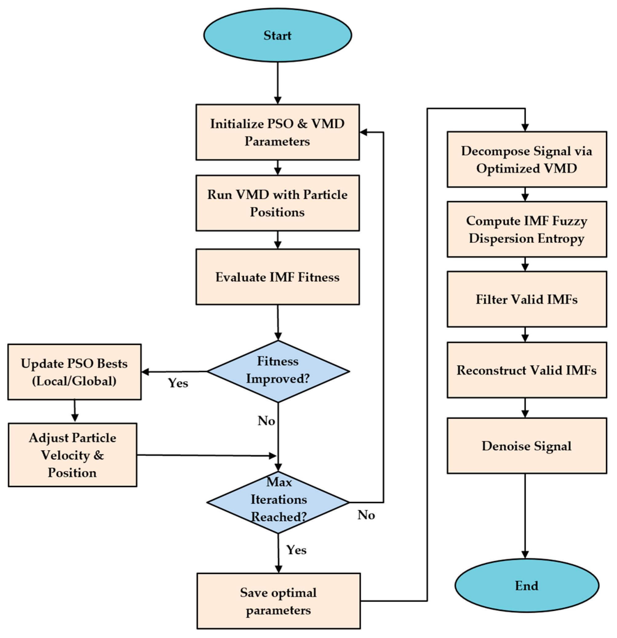
3.1. Signal Denoising Method Based on IPSO–VMD

In the process of pipeline leak detection, the acquired sensing signals often contain noise, which can adversely affect the detection process, resulting in false alarms and missed detections, etc. Therefore, it is crucial to perform noise reduction preprocessing on the detection signals to enhance the presence of leakage characteristics and improve detection accuracy. This paper proposes an improved VMD algorithm that utilizes an improved PSO algorithm to optimize the decomposition mode number K and penalty factor α. Propose a denoising method combining VMD and fuzzy dispersion entropy. The flowchart of the IPSO–VMD algorithm is shown in Figure 2.

The specific steps of IPSO–VMD are as follows:

• Preprocessing of signal $f(t_1)$ collected by DAS system using wavelet transform.
• Set the range of VMD parameters, where the value of K is set to [2–10], and α is set to [0–5000], initialize the parameters of the particle swarm optimization algorithm, where $c1$ = 2, $c2$ = 2, $c3$ = 2, $\omega$ = 0.7, sizepop = 50, and determine the fitness function $E_n$ during the optimization process [28]:

  $$\left\{\begin{array}{l}{E}_n=-{\displaystyle \sum _{i=1}^N{P}_i\log }{P}_i\\ P_i={\displaystyle \frac{a(i)}{{\displaystyle \sum _{i=1}^{N}a(i)}}}\end{array}\right.$$

  (14)
  Among them, $P_i$ is the normalized form of $a(i)$, $a(i)$ is the envelope signal obtained by Hilbert demodulation of signal $f(t_1)$.
• Initialize particle swarm to optimize parameter combinations [K, α] as the position of the particle swarm and randomly generate the initial position and movement speed of particles.
• Run VMD processing at different particle positions and calculate the fitness value $E_{\mathrm{n}}$ for each particle.
• Compare the fitness function values at different positions to obtain min$E_{\mathrm{n}}$, thereby updating individual local extremum and population global extremum. Update particle velocity and position with the Equations (8) and (9).
• Repeat steps (3) to (4) for the maximum number of iterations and output the best fitness value and the best particle position.
• Optimize [K, α] value input VMD algorithm for signal decomposition so that K IMF components can be obtained.
• Use FuzzDispEn [33] to calculate the similarity between the variance of the input signal and each IMF component, defined as follows:

  $$FuzDisEn\left[\mathrm{IMF}(i),m,c,d\right]=-{\displaystyle \sum _{\pi =1}^{c^m}P({\pi }_{v_1{v}_2\cdot \cdot \cdot v_{m-1}}})\cdot \ln P({\pi }_{v_1{v}_2\cdot \cdot \cdot v_{m-1}})$$

  (15)
• Calculate the maximum slope D of FuzzDispEn for two adjacent IMFs:

  $$\begin{array}{l}\mathrm{D}=\max \left|FuzzDispE(i)-FuzzDispE(i+1)\right|,\\ i=1,2,\cdot \cdot \cdot (K-1)\end{array}$$

  (16)
• The two adjacent modal components with the maximum increment of D are used as the turning points for selecting effective components, and the modal components with the maximum mutation of D and after are considered as noise signals. The final reconstructed signal s is obtained by adding up the effective modes.

  $$\tilde{s}={\displaystyle \sum _{m=1}^{i}IM{F}_m}$$

  (17)

This algorithm is based on MatlabR2020b, the algorithm begins with preprocessing pipeline monitoring signals (Step 1) using wavelet transform to remove noise. VMD parameters (K, α) and the particle swarm are initialized (Step 2 and 3) before optimizing these parameters using an IPSO technique (Step 5 and 6). The VMD algorithm (Step 7) is then applied to decompose the signal into IMFs. Effective IMFs are selected based on their similarity to the original signal, calculated using fuzzy dispersion entropy (Step 8 and 9). Finally, the effective IMFs are reconstructed to obtain a denoised signal (Step 10), used for threshold-based leak detection.

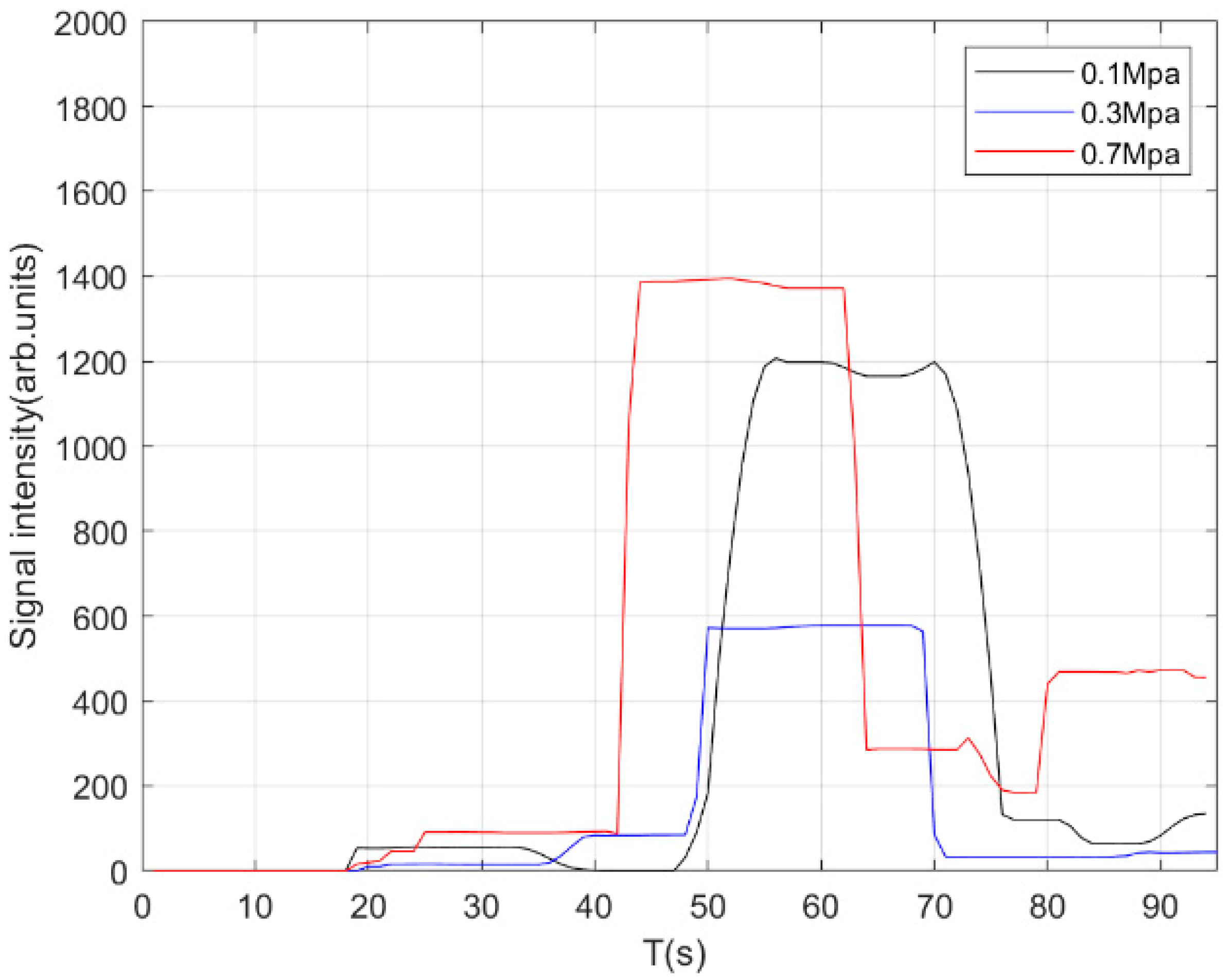
3.2. Leakage Threshold Setting

The precise setting of thresholds is crucial for effectively reducing false alarms and missed alarm rates in pipeline leakage detection. Accurately and effectively establishing system thresholds is of great practical significance in preventing false alarms and missed detections, thereby ensuring the safety and reliability of pipeline systems. Traditional methods primarily rely on determining the instantaneous value at the moment of leakage, which is often brief and susceptible to missed detections. To extend the duration of the leakage peak, this paper proposes a novel threshold setting method known as the moving standard deviation (MSD) algorithm [35]. It refers to the method of moving data with a fixed window size and calculating the standard deviation of data within the window. The specific implementation steps are as follows:

First, using the signal processed by IPSO–VMD, in order to avoid the negative value of the reconstructed signal, the negative value of the reconstructed signal is taken as 0 to obtain a new signal.

Then, the window size M is set, and the data are processed within the window using the MSD algorithm. The formula is as follows:

$$\mathrm{Std}=\sqrt{{\displaystyle \frac{{\displaystyle \sum _{i=1}^N{(x_i-\overline{x})}^2}}{\mathrm{M}-1}}}$$

(18)

The setting of M is crucial. If M is too large, it may weaken the signal strength, leading to potential misjudgment. Conversely, if M is too small, the leakage duration may be shortened, increasing the likelihood of missed detections. To determine M, data are taken to their limits, and the median is calculated, using primarily statistical and data analysis methods. Firstly, by applying extreme processing to the data, the maximum and minimum values of the data are identified, namely the upper and lower limits of the data. This step is essential for determining the data range and provides a foundation for subsequent threshold settings. After establishing the data limits, calculating the median is an important step. The median offers a better understanding of the central tendency of the data, particularly when the distribution is skewed or contains outliers. Unlike the average, the median is not influenced by extreme values, making it a more reliable indicator of the data’s central trend.

The steps are as follows:

First, it takes the minimum value of window 2 and calculates the difference between the MSD and the maximum noise value. Subsequently, the window size is extended to infinity, and the difference between the MSD and the maximum noise value is recalculated. The median of these two extreme values is then determined and compared with empirical values to establish the window size M. Statistical analysis was performed on a substantial dataset collected under varying pressures and leakage apertures. The lowest median of the two extreme values was identified as 423.336. To minimize false alarm rates, the alarm threshold was set to 80% of the lowest median, which is 338. Extensive experiments across different leakage apertures and pressures demonstrated that this threshold achieves an error accuracy of 99.5%, which can be effectively used for leak detection. Therefore, as long as the difference between the MSD and the maximum noise value in Equation (21) exceeds the alarm threshold and is maintained for 90% of the window length, it can be determined that the pipeline is leaking.

$$\mathrm{S}td-nois{e}_{\max }>338$$

(19)

4. Experimental Results and Discussion

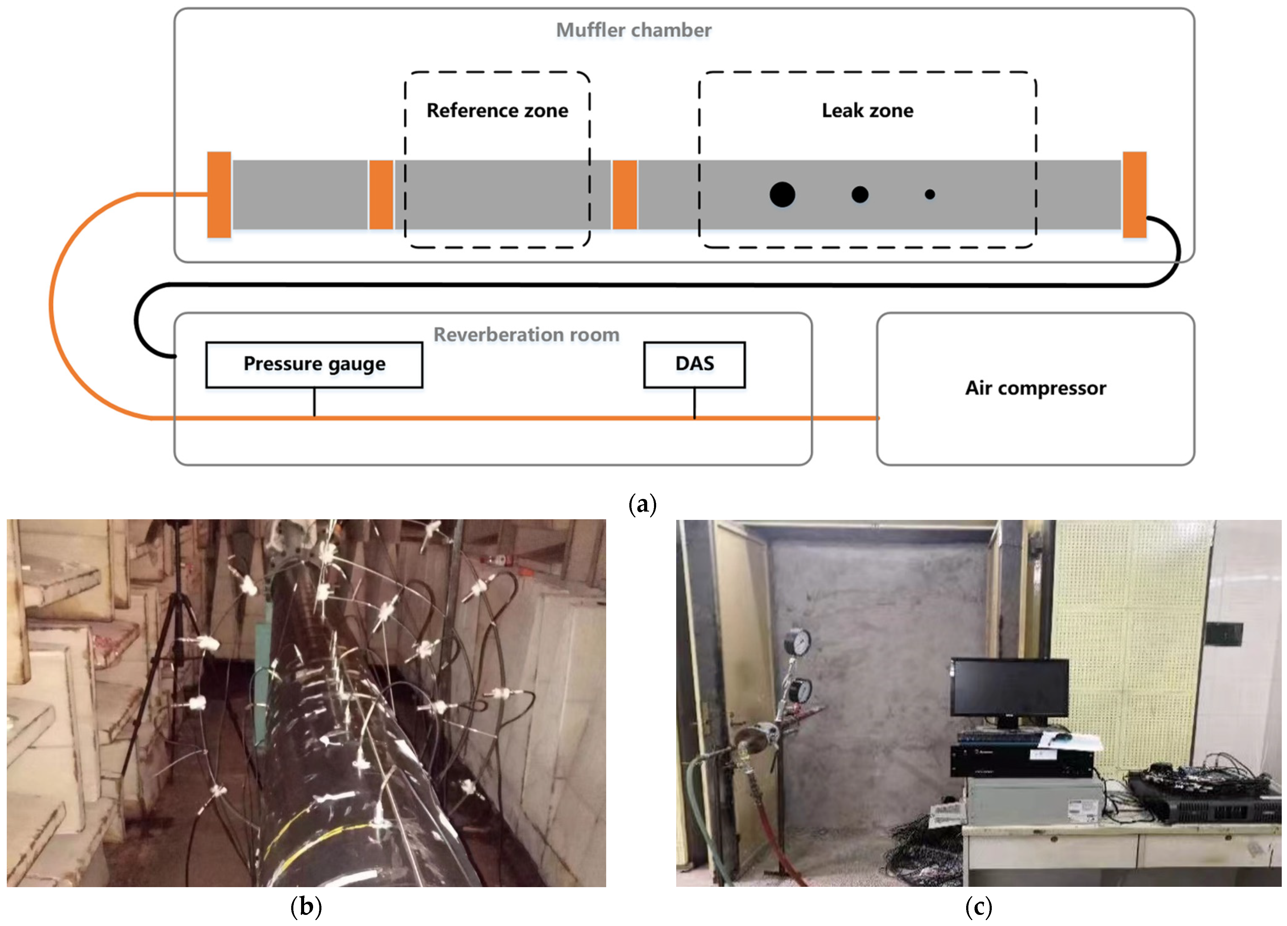
4.1. Experimental Instrumentations and Environment

The pipeline monitoring system primarily comprises a natural gas pipeline system and a fiber optic sensing system. The design of the natural gas pipeline system must align with practical engineering applications. The core of the fiber optic sensing system adopts the DAS system, which offers an innovative approach to pipeline leakage monitoring.

4.1.1. Gas Pipeline System

The DAS system is employed to detect natural gas pipeline leaks and hangs tightly packed optical fibers directly outside the pipe wall. The background noise of the full muffler room where the experiment is conducted is less than 40 dB, with frequencies below 1000 Hz, while the DAS detection system is situated in the reverberation room. The pipeline comprises three steel sections connected by flanges, as illustrated in Figure 3. It has a total length of 12.9 m and a diameter of 0.3 m. The sensing fiber used for DAS detection is directly suspended outside the pipeline [36].

The pipeline is divided into a reference area and a leak detection area. In the leak detection area, there is a simulated leak hole every 10 cm, located directly above the pipeline with diameters of 1 mm, 3 mm, and 5 mm, respectively. Both ends of the pipeline are sealed. A controllable valve is connected to the interior of pipelines via a hose and to an air compressor through pressure gauges. When the controllable valve is opened, the interior of the pipeline is pressurized using the air compressor.

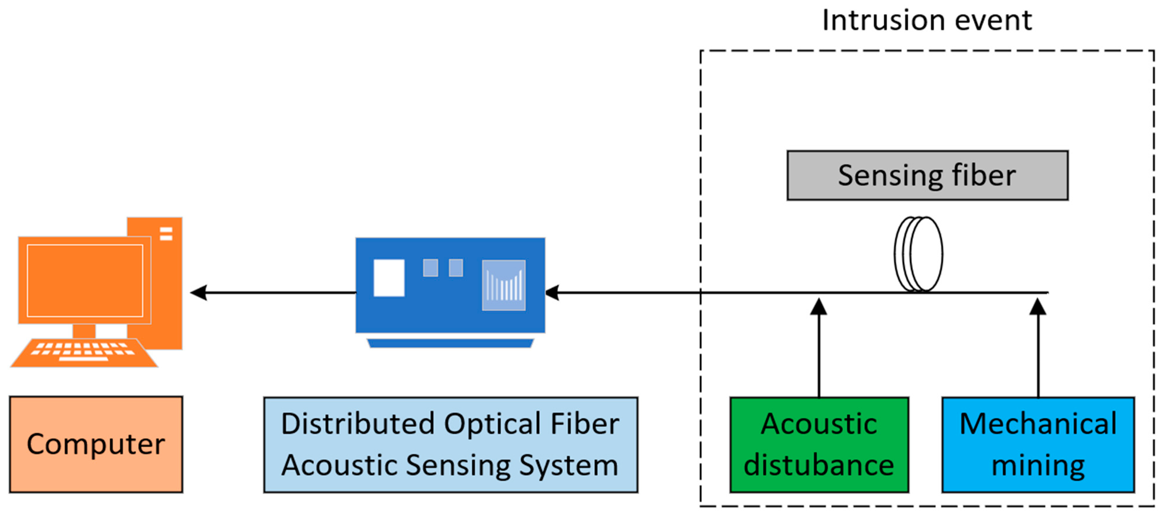
4.1.2. Fiber Optic Sensing System

The DAS system is a distributed fiber optic acoustic sensing system based on coherent Rayleigh scattering. Due to the sensitivity of sensing fibers to sound or vibration response. When an unknown intrusion event stimulates an optical fiber, the refractive index and length of the fiber will change due to the optical fiber effect, leading to a phase shift in the signal within the fiber and ultimately altering the light intensity. The fiber optic DAS system relies on the phase-sensitive Optical Time Domain Reflectometry (φ–OTDR technology, which lays the foundation for determining the location of intrusion points [37]. The detection process is shown in Figure 4. When an intrusion event (such as acoustic disturbance or mechanical excavation) occurs, the sound or vibration stimulates the optical fiber. The DAS system captures the sensing signals, which are subsequently processed by a computer. The improved algorithm proposed in this paper is specifically designed for noise reduction of the raw sensing signals acquired by the DAS system.

The detection fiber in DAS sensing system utilizes single-mode tightly packed fiber. As shown in Figure 3b, the probe optical fiber is suspended at one side of the pipeline, positioned 0.05 m from the pipe wall. To mitigate the influence of external factors, 20-m-long fiber rings at both ends of the pipeline are wrapped in the muffler cotton. Longer pulse lengths enhance the sensitivity to signals caused by leaks but reduce spatial resolution. A pulse length of 50 ns corresponds to a spatial resolution of approximately 5 m in optical fibers [38], enabling the localization of pipeline leaks. The pulse repetition frequency, which determines the maximum frequency of detectable signals, is set to a maximum value of 20 kHz in the DAS system to broaden the frequency range. To improve the sensitivity and linear stability of the system, the detection time is set to 3 min, with a detection fiber length of 1000 m [39].

During the experiment, both the size of the leakage hole and the pressure within the pipeline are comprehensively considered. For each experiment, the pressure is initially set to a predetermined value 0.1–0.7 Mpa. The pressure in the pipeline is increased to this predetermined value, and the leakage hole is opened once the pressure stabilizes. Simultaneously, a 3-min test is conducted using the DAS system, during which the pressure inside the pipe gradually decreases due to gas leakage.

To enhance applicability in practical scenarios, the sensing fiber adopts a tightly wrapped fiber optic overhead laying method, which differs from bare fiber optic laying and is more suitable for engineering applications. Sensing data is collected over a 3-m-long optical fiber segment, as opposed to a single point, thereby improving the calibration accuracy to meet engineering requirements.

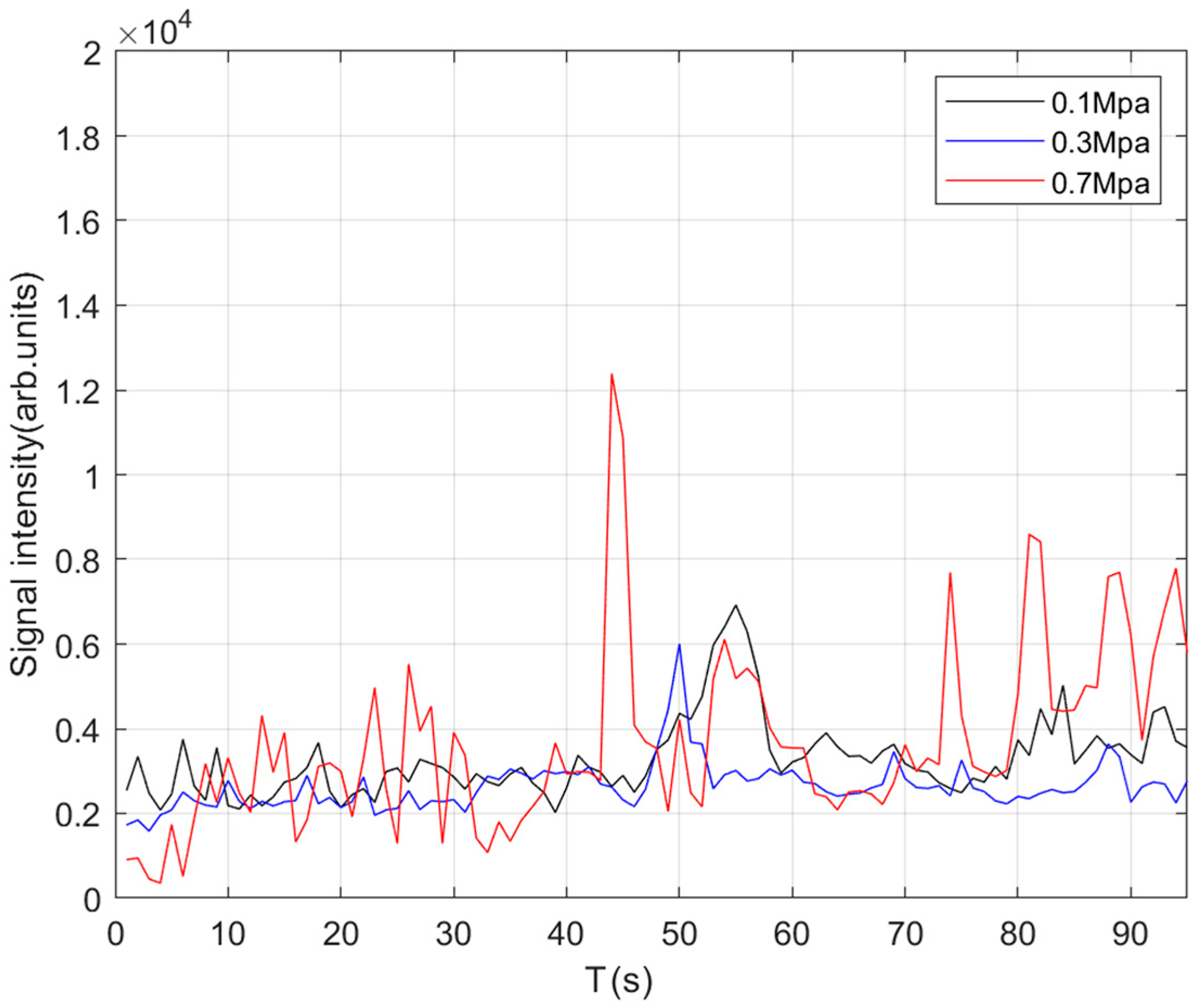
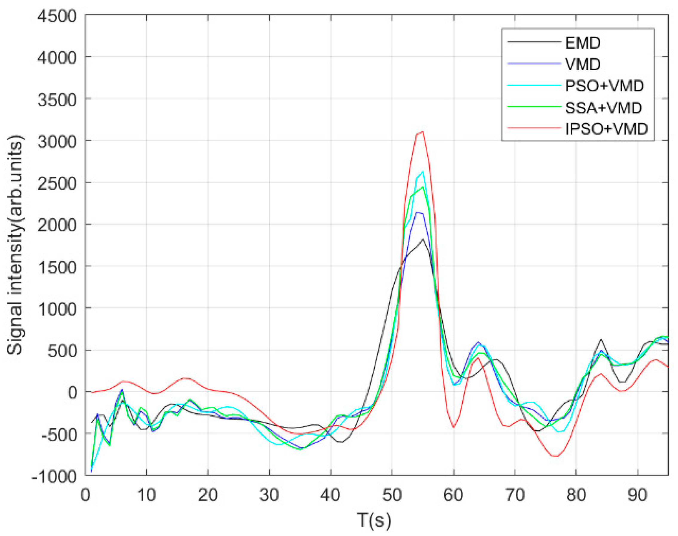
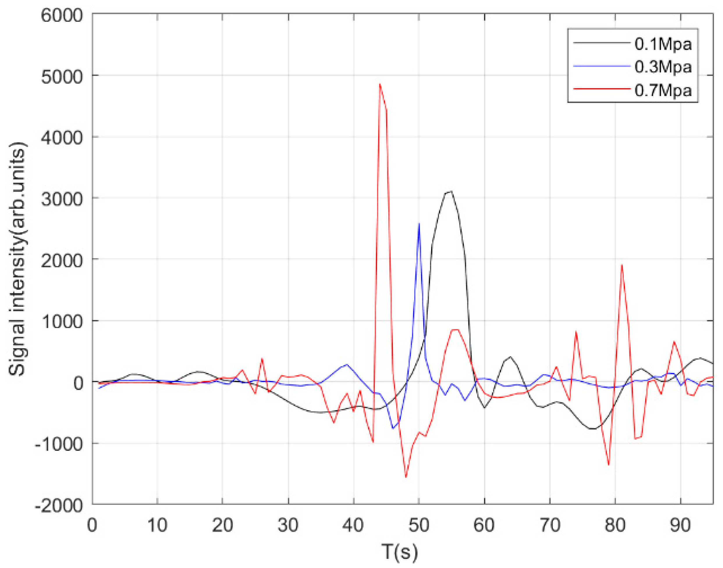
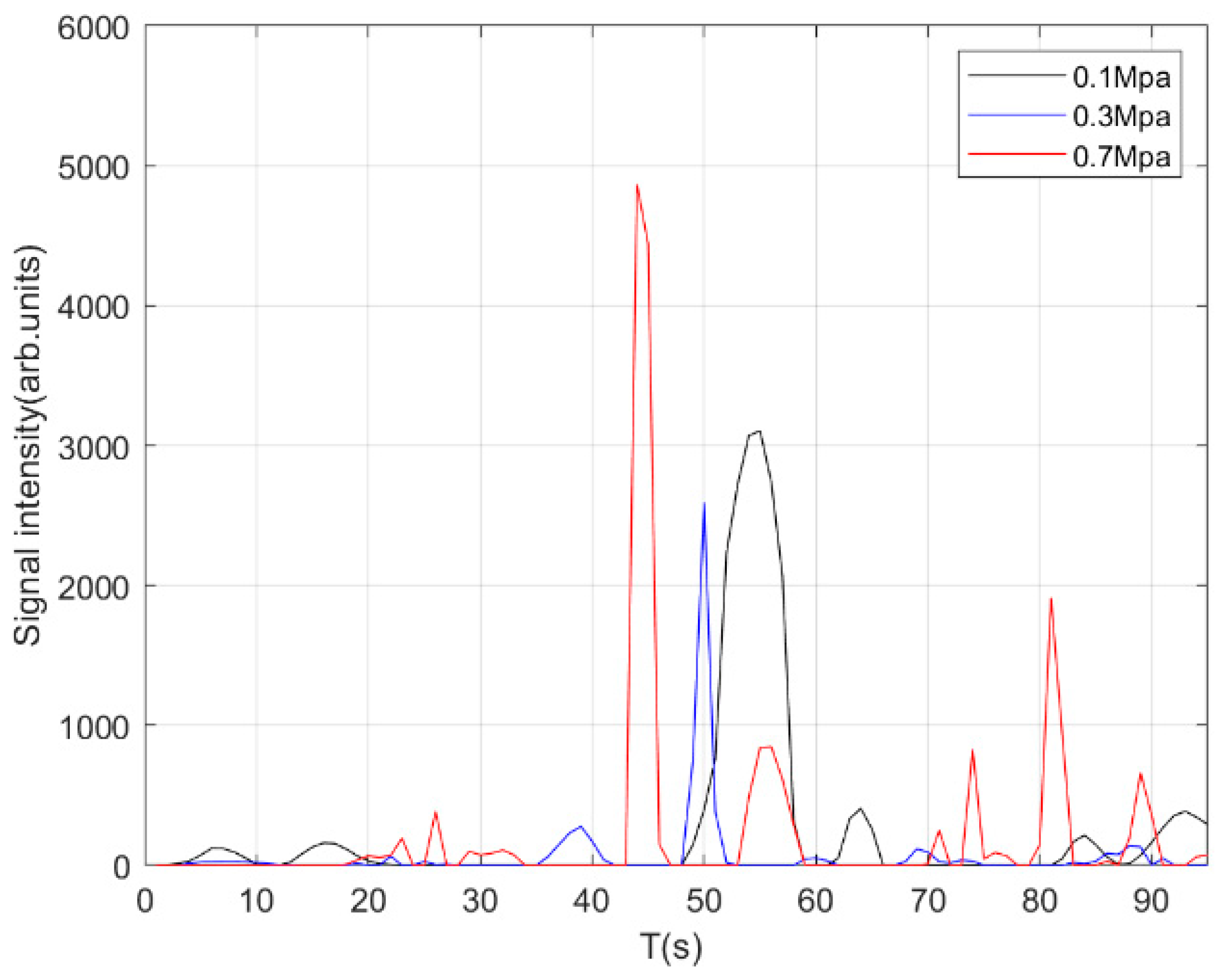
4.2. Results and Analysis Based on IPSO–VMD

Figure 5 illustrates the original time-domain signal for a leakage aperture of 1 mm at pipeline pressures of 0.1 Mpa, 0.3 Mpa, and 0.7 Mpa, respectively. The test signal is a continuously monitored signal, and a total of 90 s of continuous monitoring of the received signal was recorded. The pipeline leakage occurs at 55 s, 50 s, and 44 s, respectively, making it challenging to distinguish the useful pipeline leakage signals.

To verify the superiority of the proposed algorithm IPSO–VMD, this paper uses the original data at 0.1 Mpa as an example. Taking 0.1 MPa as an example, multiple tests conducted at this pressure level demonstrate that, despite variations among individual samples, similar leak signals are consistently obtained, indicating a satisfactory level of consistency and good repeatability. EMD, VMD, PSO, SSA, and IPSO–VMD were used to reconstruct the original signal, respectively, and the reconstructed signal was shown in Figure 6. Prior to applying these five algorithms, wavelet transform processing is performed. From the figure, the reconstructed signal by IPSO–VMD can retain the leaked information well and reduce the interference of sidelobe signal effectively. The leakage characteristics of IPSO–VMD algorithm are the most pronounced.

Mean square error (MSE) and signal-to-noise ratio (SNR) are commonly used to evaluate the de-noising effect; the specific formulas are shown in Equations (20) and (21). The SNR is used to measure the clarity and purity of a signal, MSE is used to measure the difference between predicted or restored results and the true values. A higher SNR and a lower MSE after de-noised signal indicate a better de-noising effect [19].

Table 1. MSE and SNR of simulated signals.

Method	MSE	SNR (dB)
EMD	0.0147	18.28
VMD	0.0097	19.96
PSO + VMD	0.0060	21.99
SSA + VMD	0.0068	21.38
IPSO + VMD	0.0027	24.15

compares the MSE and SNR values of five different algorithms. The table shows that the IPSO–VMD method proposed in this paper achieves the highest signal-to-noise ratio of 24.15 dB and the lowest mean square error of 0.0027.

$$\mathrm{SNR}=10 \lg \left({\displaystyle \sum _{i=1}^N{x_i}^2}/{\displaystyle \sum _{i=1}^N{(x_i-{\widehat{x}}_i)}^2}\right)$$

(20)

$$MSE={\displaystyle \frac{1}{N}}{\displaystyle \sum _{i=1}^N{({\widehat{x}}_i-x_i)}^2}$$

(21)

where $x_i$ is the pure signal, ${\widehat{x}}_i$ is the denoised signal, and N is the signal length.

In theory, IPSO can search for the global optimal solution more efficiently by improving the PSO. VMD can decompose complex signals into multiple modalities, which helps extract key features from the signal. IPSO–VMD combines the advantages of both, further improving the accuracy of signal processing. In practice, IPSO–VMD exhibits low error and high stability under different conditions. In summary, the IPSO–VMD outperforms other algorithms in both theory and practice, mainly due to its powerful optimization and signal processing capabilities, as well as its high precision and robustness demonstrated in practical applications.

Utilize the IPSO–VMD algorithm proposed in this paper to process monitoring signals, with a leakage aperture of 1 mm. Then, obtain the reconstructed time-domain signals at pressures of 0.1 Mpa, 0.3 Mpa, and 0.7 Mpa, respectively. As shown in Figure 7, the characteristic signals of pipeline leakage are evident at the 55th, 50th, and 44th seconds. The features of the reconstructed signals are basically consistent with the characteristic basis of the original time-domain signals. The improved algorithm proposed in this paper demonstrates strong anti-interference capabilities, enhances the extraction of useful signals, and improves positioning accuracy. In practical applications, it can significantly improve the efficiency and accuracy of underground pipeline leak detection. Provided effective technical methods for leak detection of underground pipelines, thereby ensuring the safe operation of gas pipelines. It also lays a solid foundation for subsequent signal analysis and leak localization.

4.3. Leakage Localization

According to the threshold setting method, the negative values of the reconstructed signal are initially set to zero to obtain a new signal under three pressure conditions, as shown in Figure 8. This step is crucial to prevent any potential impact of negative values on the results.

According to the methods mentioned in Section 3, the window size is set to 20. The data within this window are processed using the Moving standard deviation algorithm, with results depicted in Figure 9. As shown in Figure 9, the differences between the moving standard deviation and the maximum noise value at pressures of 0.1 Mpa, 0.3 Mpa, and 0.7 Mpa, which are 1132.138, 488.5939, 1296.5806, respectively, occurring at 55 s, 50 s, and 44 s. All values exceeded the alarm threshold of 185, and the values 1132.138, 488.5939, 1296.5806 persist for 18 s, confirming that the pipeline has leaked at 55 s, 50 s, 44 s, respectively. This is consistent with the actual leak occurrence times.

The leakage signal detection time can last for 18 s, effectively reducing missed and false alarms, improving the accuracy of gas pipeline leakage detection, lowering false alarm rates, and enabling timely and effective measures to prevent and mitigate leakage incidents. This is of great significance for practical applications. Although the improved algorithm proposed in this study demonstrates effective performance in denoising gas pipeline leakage signals, the extraction of weak pipeline signals remains challenging under complex working conditions and strong background noise interference. This difficulty may be attributed to the algorithm’s limitations in handling high–frequency noise, which can lead to signal distortion or inadequate denoising. Further research is required to integrate multiple signal processing methods for analyzing leakage signals, with the goal of enhancing the denoising performance and feature extraction capability for such signals. The algorithm proposed in this paper demonstrates robust capabilities in signal processing and feature extraction. Its application scope extends beyond pipeline leak detection to various other industries and fields. For example, in the early fault detection of mechanical components such as rolling bearings and gearboxes, the application of this algorithm can enhance the accuracy and reliability of fault diagnosis.

5. Conclusions

Leakage in transportation pipelines is a significant cause of major hazardous incidents at oil and gas chemical terminals, potentially leading to catastrophies such as fires and explosions. These incidents not only threaten human life and property but also cause severe marine environmental pollution and substantial economic losses. This paper aims to address these challenges by developing advanced denoising and detection models to significantly improve the accuracy of gas pipeline leak detection, reduce false alarms and omissions, and provide a robust theoretical foundation for ensuring safe and stable gas transportation. The proposed pipeline leak detection algorithm, based on IPSO–VMD, achieves a SNR of 24.15 dB and reduces the MSE to 0.0027, demonstrating superior performance in noise reduction and signal clarity. Furthermore, a novel threshold setting method is introduced to overcome the limitations of traditional approaches that rely on instantaneous values for leak detection. This approach effectively reduces the false alarm rate while maintaining high detection accuracy and strong practical applicability. The proposed approach not only enhances the safety and reliability of pipeline monitoring but also offers significant economic and environmental benefits by minimizing marine pollution and reducing the risk of leakage incidents at oil and gas terminals. By supporting rapid economic growth and fostering sustainable social development, this method represents a critical advancement in pipeline safety technologies.

Despite these advancements, it is important to acknowledge the limitations of this study. The experimental setup was conducted in a controlled environment, which may not fully capture the complexities of real–world pipeline conditions. Factors such as the shape of the leakage hole, environmental noise, and their potential impact on sensor performance were not considered in this work. Additionally, the influence of temperature on the DAS system was not explicitly addressed. While temperature-induced intensity variations are negligible compared to those caused by acoustic disturbances, and pipelines in practical engineering environments are typically buried underground with minimal temperature fluctuations, the potential effects of temperature on system performance warrant further investigation. Future research should focus on addressing these limitations by conducting experiments in more complex pipeline configurations and integrating artificial intelligence (AI) algorithms to achieve automated, efficient, and accurate identification of pipeline leaks. These efforts will enhance the practical applicability of the leak detection system and pave the way for its deployment in diverse real–world scenarios.

The broader implications of this research extend beyond pipeline safety. By advancing the capabilities of DAS systems and optimization algorithms, this study contributes to the development of intelligent monitoring technologies for critical infrastructure. The integration of AI and machine learning techniques holds promise for transforming pipeline monitoring into a proactive, data-driven process, ultimately reducing the risk of accidents and ensuring the sustainable operation of oil and gas transportation networks. This research not only addresses immediate technical challenges but also inspires future innovations in the field, fostering ongoing academic dialogue and industrial collaboration.

References

1. Latif, J.; Shakir, M.Z.; Edwards, N.; Jaszczykowski, M.; Ramzan, N.; Edwards, V. Review on condition monitoring techniques for water pipelines. Measurement 2022, 193, 110895. [Google Scholar] [CrossRef]
2. Manogharan, P.; Rivière, J.; Shokouhi, P. Toward In-situ characterization of additively manufactured parts using nonlinear resonance ultrasonic spectroscopy. Res. Nondestruct. Eval. 2022, 33, 243–266. [Google Scholar] [CrossRef]
3. Li, G.; Zeng, K.; Zhou, B.; Yang, W.; Lin, X.; Wang, F.; Chen, Y.; Ji, X.; Zheng, D.; Mao, B.-M. Vibration monitoring for the West-East Gas Pipeline Project of China by phase optical time domain reflectometry (phase-OTDR). Instrum. Sci. Technol. 2020, 49, 65–80. [Google Scholar] [CrossRef]
4. Tomassi, A.; de Franco, R.; Trippetta, F. High-resolution synthetic seismic modelling: Elucidating facies heterogeneity in carbonate ramp systems. Pet. Geosci. 2025, 31, petgeo2024-047. [Google Scholar] [CrossRef]
5. Philibert, M.; Yao, K.; Gresil, M.; Soutis, C. Lamb waves-based technologies for structural health monitoring of composite structures for aircraft applications. Eur. J. Mater. 2022, 2, 436–474. [Google Scholar] [CrossRef]
6. Butterfield, J.D.; Krynkin, A.; Collins, R.P.; Beck, S.B.M. Experimental investigation into vibro-acoustic emission signal processing techniques to quantify leak flow rate in plastic water distribution pipes. Appl. Acoust. 2017, 119, 146–155. [Google Scholar] [CrossRef]
7. Wang, J.; Ren, L.; Jia, Z.; Jiang, T.; Wang, G.-X. A novel pipeline leak detection and localization method based on the FBG pipe-fixture sensor array and compressed sensing theory. Mech. Syst. Signal Process. 2022, 169, 108669. [Google Scholar] [CrossRef]
8. Siddique, M.F.; Ahmad, Z.; Kim, J.-M. Pipeline leak diagnosis based on leak-augmented scalograms and deep learning. Eng. Appl. Comput. Fluid Mech. 2023, 17, 2225577. [Google Scholar] [CrossRef]
9. Ahmad, Z.; Nguyen, T.-K.; Kim, J.-M. Leak detection and size identification in fluid pipelines using a novel vulnerability index and 1-D convolutional neural network. Eng. Appl. Comput. Fluid Mech. 2023, 17, 2165159. [Google Scholar] [CrossRef]
10. Xiao, R.; Hu, Q.; Li, J. Experimental investigation on vibro-acoustic techniques to detect and locate leakages in gas pipelines. Meas. Sci. Technol. 2021, 32, 114004. [Google Scholar] [CrossRef]
11. Tu, Q.C.; Wei, B.; Zhang, Z.Y.; Shi, X.B. OTDR-type Distributed Optical Fiber Sensors and Application of Oil and Gas Pipelines Online Monitoring. Pipeline Technol. Equip. 2015, 3, 28–31. [Google Scholar]
12. Tong, J.K.; Jin, B.Q.; Wang, D.; Wang, Y.; Hui, Y.; Bai, L. Distributed Optical Fiber Temperature Measurement System for Pipeline Safety Monitoring Based on R-OTDR. Chin. J. Sens. Actuators 2018, 31, 158–162. [Google Scholar] [CrossRef]
13. Muanenda, Y. Recent advances in distributed acoustic sensing based on phase-sensitive optical time domain reflectometry. J. Sens. 2018, 2018, 3897873. [Google Scholar] [CrossRef]
14. Stajanca, P.; Chruscicki, S.; Homann, T.; Seifert, S.; Schmidt, D.; Habib, A. Detection of leak-induced pipeline vibrations using fiber—Optic distributed acoustic sensing. Sensors 2018, 18, 2841. [Google Scholar] [CrossRef] [PubMed]
15. Wu, H.; Duan, H.F.; Lai, W.W.; Zhu, K.; Cheng, X.; Yin, H.; Zhou, B.; Lai, C.C.; Lu, C.; Ding, X. Leveraging optical communication fiber and AI for distributed water pipe leak detection. IEEE Commun. Mag. 2023, 62, 126–132. [Google Scholar] [CrossRef]
16. Guo, C.; Wen, Y.; Li, P.; Wen, J. Adaptive noise cancellation based on EMD in water-supply pipeline leak detection. Measurement 2016, 79, 188–197. [Google Scholar] [CrossRef]
17. Li, Y.; Li, Y.; Chen, X.; Yu, J. Denoising and feature extraction algorithms using NPE combined with VMD and their applications in ship-radiated noise. Symmetry 2017, 9, 256. [Google Scholar] [CrossRef]
18. Dragomiretskiy, K.; Zosso, D. Variational mode decomposition. IEEE Trans. Signal Process. 2014, 62, 531–544. [Google Scholar] [CrossRef]
19. Lu, J.; Yue, J.; Zhu, L.; Li, G. Variational mode decomposition denoising combined with improved Bhattacharyya distance. Measurement 2019, 151, 107283. [Google Scholar] [CrossRef]
20. Peng, L.; Hu, Y.; Zhang, J.; Lin, J. Pipeline leak location method based on SSA-VMD with generalized quadratic cross-correlation. Meas. Sci. Technol. 2024, 35, 116105. [Google Scholar] [CrossRef]
21. Du, H.; Wang, J.; Qian, W.; Zhang, X. An Improved Sparrow Search Algorithm for the Optimization of Variational Modal Decomposition Parameters. Appl. Sci. 2024, 14, 2174. [Google Scholar] [CrossRef]
22. Jiang, Z.; Guo, G.; Liu, B. Application research of negative pressure wave signal denoising method based on VMD. Appl. Sci. 2023, 13, 4156. [Google Scholar] [CrossRef]
23. Diao, X.; Jiang, J.; Shen, G.; Chi, Z.; Wang, Z.; Ni, L.; Mebarki, A.; Bian, H.; Hao, Y. An improved variational mode decomposition method based on particle swarm optimization for leak detection of liquid pipelines. Mech. Syst. Signal Process. 2020, 143, 106787. [Google Scholar] [CrossRef]
24. Hahn, S.L. Hilbert Transforms in Signal Processing; Artech House Publish: Boston, MA, USA, 1996. [Google Scholar]
25. Duan, J.Y.; Duan, T.Y.; Liu, H.; Jiang, T.F.; Jin, X.X. Application of variational mode decomposition in denoising of microseismic signals. Petrochem. Technol. 2015, 22, 217. [Google Scholar]
26. Xiao, Q.; Li, J.; Sun, J.; Feng, H.; Jin, S. Natural-gas pipeline leak location using variational mode decomposition analysis and cross-time–frequency spectrum. Measurement 2018, 124, 163–172. [Google Scholar] [CrossRef]
27. Huang, W.; Jiang, Y.; Sun, H.; Wang, W. Automatic quantitative diagnosis for rolling bearing compound faults via adapted dictionary free orthogonal matching pursuit. Measurement 2020, 154, 107474. [Google Scholar] [CrossRef]
28. Tang, G.; Wang, X. Parameter Optimization Variational Mode Decomposition Method in Rolling Application of early fault diagnosis in dynamic bearings. Xi’an Jiaotong Univ. J. 2015, 49, 73–81. [Google Scholar]
29. Nguyen, V.D.; Tran, Q.D.; Vu, Q.T.; Duong, V.T.; Nguyen, H.H.; Hoang, T.T.; Nguyen, T.T. Force Optimization of Elongated Undulating Fin Robot Using Improved PSO-Based CPG. Comput. Intell. Neurosci. 2022, 2022, 2763865. [Google Scholar] [CrossRef]
30. Del Valle, Y.; Venayagamoorthy, G.K.; Mohagheghi, S.; Hernandez, J.C.; Harley, R.G. Particle swarm optimization: Basic concepts, variants and applications in power systems. IEEE Trans. Evol. Comput. 2008, 12, 171–195. [Google Scholar] [CrossRef]
31. Eberhart, R.C.; Shi, Y.; Kennedy, J. Swarm Intelligence (Morgan Kaufmann Series in Evolutionary Computation); Morgan Kaufmann Publishers: Burlington, MA, USA, 2001. [Google Scholar]
32. Cho, M.-Y.; Hoang, T.T. Feature selection and parameters optimization of SVM using particle swarm optimization for fault classification in power distribution systems. Comput. Intell. Neurosci. 2017, 2017, 4135465. [Google Scholar] [CrossRef]
33. Rostaghi, M.; Khatibi, M.M.; Ashory, M.R.; Azami, H. Fuzzy dispersion entropy: A nonlinear measure for signal analysis. IEEE Trans. Fuzzy Syst. 2021, 30, 3785–3796. [Google Scholar] [CrossRef]
34. Li, Y.; Tang, B.; Geng, B.; Jiao, S. Fractional order fuzzy dispersion entropy and its application in bearing fault diagnosis. Fractal Fract. 2022, 6, 544. [Google Scholar] [CrossRef]
35. Nair, V.S.; Rameshkumar, K.; Saravanamurugan, S. Chatter identification in turning of difficult-to-machine materials using moving window standard deviation and decision tree algorithm. J. Ceram. Process. Res. 2022, 23, 503–510. [Google Scholar]
36. Zuo, J.; Zhang, Y.; Xu, H.; Zhu, X.; Zhao, Z.; Wei, X.; Wang, X. Pipeline leak detection technology based on distributed optical fiber acoustic sensing system. IEEE Access 2020, 8, 30789–30796. [Google Scholar] [CrossRef]
37. Juškaitis, R.; Mamedov, A.M.; Potapov, V.T.; Shatalin, S.V. Interferometry with Rayleigh backscattering in a single-mode optical fiber. Opt. Lett. 1994, 19, 225–227. [Google Scholar] [CrossRef] [PubMed]
38. Liu, J. Research progress on distributed fiber optic sensing and monitoring technology using φ-OTDR. Laser Optoelectron. Prog. 2013, 50, 80021-1. [Google Scholar]
39. Li, R.; He, D. Rotational machine health monitoring and fault detection using EMD-based acoustic emission feature quantification. IEEE Trans. Instrum. Meas. 2012, 61, 990–1001. [Google Scholar] [CrossRef]
Figure 1. Schematic of particle swarm optimization iterative update equations.
Jmse 13 00531 g001
Figure 2. Flowchart of improved PSO–VMD algorithm for pipeline leakage signal denoising.
Jmse 13 00531 g002
Figure 3. Experimental instrumentations and environment. (a) Schematic diagram of natural gas pipeline system; (b) Experimental pipeline and environment; (c) DAS system.
Jmse 13 00531 g003
Figure 4. Diagram of pipeline leakage detection system.
Jmse 13 00531 g004
Figure 5. Original time–domain signals with leakage aperture of 1 mm and pressure of 0.1 Mpa, 0.3 Mpa, and 0.7 Mpa.
Jmse 13 00531 g005
Figure 6. Reconstructed signal by EMD, VMD, PSO, SSA, and IPSO–VMD under 0.1 Mpa.
Jmse 13 00531 g006
Figure 7. Reconstructed time–domain signals with leakage aperture of 1 mm and pressure of 0.1 Mpa, 0.3 Mpa and 0.7 Mpa.
Jmse 13 00531 g007
Figure 8. Take 0 as negative value under three pressures.
Jmse 13 00531 g008
Figure 9. Moving standard deviation of the new signal at 0.1 Mpa, 0.3 Mpa, and 0.7 Mpa.
Jmse 13 00531 g009