Abstract
The placement of artificial reefs (ARs) significantly influences local hydrodynamics and nutrient transport, both of which are crucial for enhancing marine ecosystems and improving marine habitats. Large eddy simulations (LESs) are performed to study the flow field around a cuboid artificial reef (CAR) with three inflow angles ( = 0°, 45°, and 90°). The numerical method is successfully validated with experimental data, and a reasonable grid resolution is chosen. The results demonstrate that the case with an inflow angle of 45° exhibits superior flow field performance, including the largest recirculation bubble length and the maximum volumes for both the upwelling and wake regions. Stronger turbulence is also observed around the CAR at this inflow angle, attributed to the intensified shear layer. The instantaneous flow features torn horseshoe vortices and rollers shed from the shear layer, which further develop into hairpin vortices.
1. Introduction
The marine ecological environment and biological resources are increasingly threatened by accelerated climate change, deteriorating water quality, and modern fishing practices [1,2,3,4]. Recently, artificial reefs (ARs), human-made submerged structures, have garnered considerable interest due to their notable successes in the preservation of marine ecosystems and enhancing oceanic environments [5,6,7]. The presence of ARs in marine environments significantly alters the local hydrodynamics, providing shelter for marine species and modifying the circulation of sediments and nutrients [8,9,10]. Therefore, a thorough understanding of the flow dynamics around ARs is essential for the restoration and enhancement of marine ecosystems.
Generally, two key regions are formed in the surrounding area of ARs when AR units are placed on the seabed: the upwelling region and the wake region [11,12,13]. The upwelling region is located upstream of ARs and is defined as the area where the vertical velocity, , is greater than or equal to 10% of the inlet velocity, [14,15]. This region promotes the exchange of materials between different water layers and facilitates the accumulation of organic matter [16]. The second region, referred to as the wake region, forms downstream of ARs and is characterized by a streamwise velocity, , that is negative [17,18]. This low-momentum wake region provides shelter, foraging, and spawning spaces for fish species. Extensive research has been conducted, and design parameters, such as shapes and configurations, have been found to significantly affect the flow characteristics of these two regions around ARs. Specifically, Kim et al. [19] numerically investigated the relationship between 24 representative ARs and their wake regions, finding that the AR type and reference plane strongly govern the size of the wake length. Wang et al. [18] used the ANSYS Fluent 2012R1 to compare the flow field performances between Menger-type ARs and traditional ARs. The numerical results suggested that the Menger-type ARs outperform traditional ARs in terms of flow characteristics in both the upwelling and wake regions. Two different configurations of ARs were investigated both experimentally and numerically, and the AR with a hole diameter of 0.25 m demonstrated better performance than the one with a hole diameter of 0.5 m in terms of improving the circulation of water and nutrients [13]. Maslov et al. [20] proposed a novel design for artificial reefs (ARs), comparing the performances of droplet and circular cross sections using four evaluation indices. Their findings revealed that the droplet cross section exhibited superior flow field performance and higher efficiency compared with the circular cross section. Moreover, the arrangement and deployment of ARs are effective strategies for altering the hydraulic characteristics around ARs. Liu et al. [11] demonstrated that the interference effect between the ARs persists when the transverse distance between the ARs is less than twice the length of the ARs. The low-velocity zone between the ARs in the longitudinal direction is positively correlated with the distance between them. Shu et al. [21] experimentally examined the impact of spacing between M-shaped artificial reefs (ARs) on turbulent intensity. Their results indicated that the low-turbulence region was situated upstream of the ARs, while the downstream area displayed increased turbulence.
The aforementioned research efforts are highly valuable for the design and optimization of ARs, and these investigations primarily rely on numerical simulations rather than laboratory experiments. This preference is due to the cost-effectiveness and time efficiency of numerical simulations, making them more practical compared with laboratory experiments or field monitoring. In past studies, many computational fluid dynamics (CFD) cases have focused on Reynolds-averaged Navier–Stokes (RANS) models, such as the k– model [11,13,18,22] and the k– model [20]. The flow through ARs is highly complex due to interactions between the flow and obstacles, which induce turbulence and the formation of three-dimensional coherent structures. These turbulent flow structures influence the swimming behavior, aggregation, and migration of fish species, as well as the transport rates of sediments and nutrients [23,24,25]. However, the limitation of the RANS model is that it may lose the instantaneous turbulent flow fields due to the averaging of turbulent information [26,27]. Additionally, another physical process related to flow separation requires further investigation, as the vortices and eddy currents formed in the wake region by flow separation are also factors influencing fish aggregation [28,29,30]. Unsteady Reynolds-averaged Navier–Stokes (URANS) models have been found to be slightly inaccurate in predicting the flow separation and reattachment [31,32,33]. Thus, a high-fidelity, detailed numerical simulation tool is essential to reveal the three-dimensional (3D) hydrodynamics of such complex flow. Recently, large eddy simulation (LES) has been widely used to study the flow through or around obstacles in open-channel and oceanic flows [34,35,36]. The LES method not only provides the necessary resolution of turbulent structures, but also accurately predicts regions of flow separation [37,38,39].
Very few studies have explored the turbulence structures and flow separation around artificial reefs (ARs), particularly under varying inflow angles, even though these factors play a crucial role in the flow dynamics around or through these submerged structures. Zhang et al. [40] evaluated the impact of the layout configuration of ARs using CFD methods and proposed an optimal spacing distance. Their findings revealed that the inflow angle has the most significant influence on the flow field around ARs, surpassing the effects of the longitudinal and transverse intervals between ARs.
This study employs large eddy simulation (LES) to ascertain the hydrodynamics and turbulence of flow through artificial reefs (ARs) at different angles of attack. This paper is structured as follows: Section 2 describes the numerical methods and setup, including the validation case. Section 3 presents and analyzes the results, encompassing time-averaged and instantaneous flow and turbulence parameters, as well as upwelling and wake region characteristics. Section 4 concludes with a summary and final remarks.
2. Methodology
In this study, high-resolution large eddy simulations were conducted using the open-source code Hydro3D v6.0, which has been widely applied and validated for simulating complex and challenging flow scenarios [41,42,43,44]. The code solves spatially filtered Navier–Stokes equations for incompressible viscous flow in a Eulerian framework,
where and are filtered velocity vectors (i and j = 1, 2, and 3 represent the x-, y-, and z- axis directions, respectively); similarly, and represent the spatial location vectors in the three directions; p and are the pressure and kinematic viscosity of the fluid, respectively; and represents the sub-grid scale stress.
In Hydro3D, the sub-grid scale stress tensor is calculated using the wall-adapting local eddy (WALE) viscosity model, as proposed by Nicoud and Ducros [45]. Fourth- and second-order central differences schemes are used to approximate convective and diffusive terms, respectively. Time advancement is performed using a fractional step method, with a three-step Runge–Kutta scheme to obtain second-order accuracy. In the final step, a Poisson pressure correction equation is applied to couple the pressure field with the velocity field. Hydro3D is based on finite differences, and the filtered equations were solved on a uniform Cartesian grid. The immersed boundary method (IBM) is employed to enforce the no-slip condition on submerged bodies, such as the cuboid artificial reef (CAR) in this study.
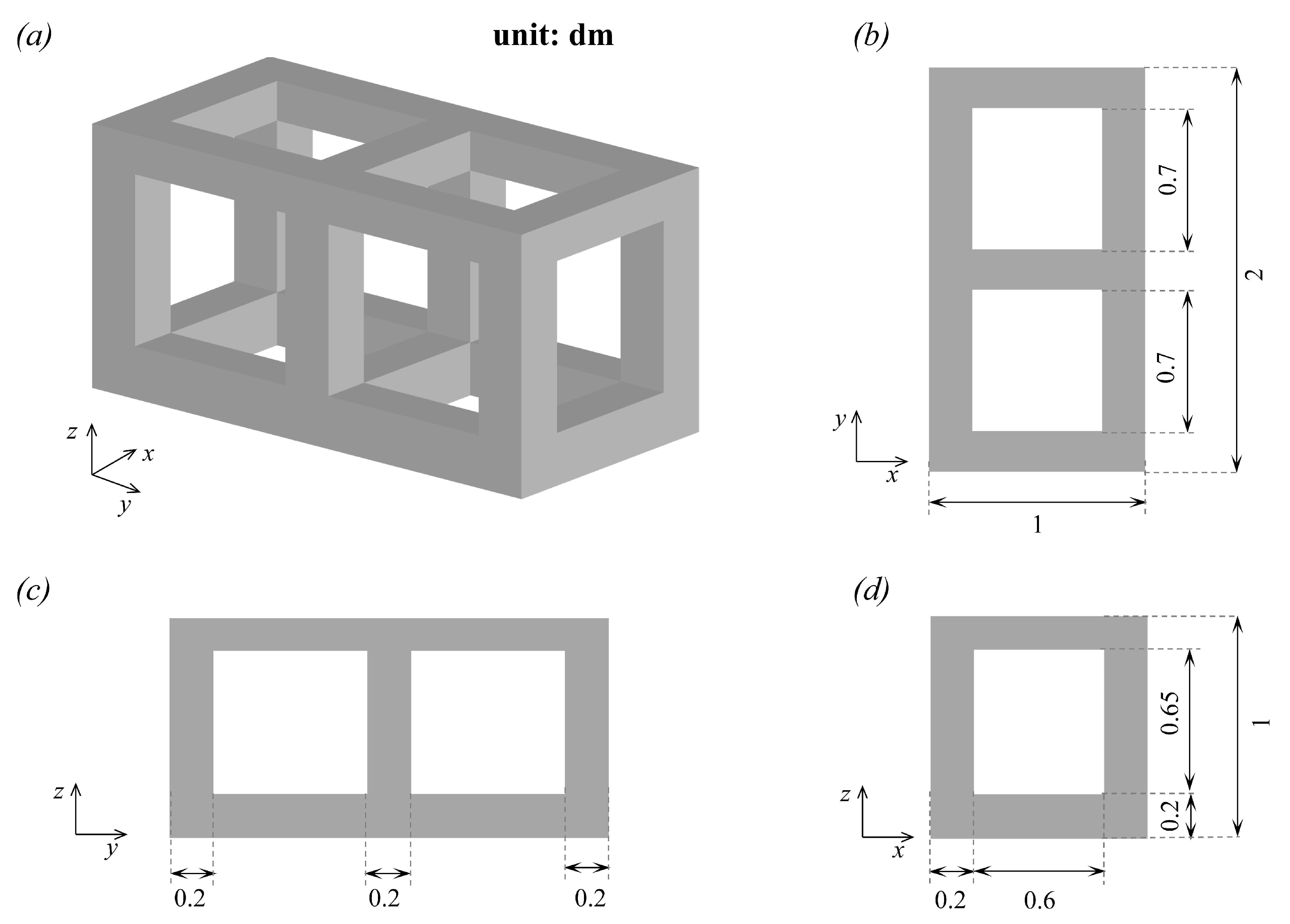
The setup of LES is analogous to the experimental study carried out by Tan et al. [46]. The experiments were conducted in a flume with dimensions of m (length × width × height). A 1:10 scale model was constructed to represent the prototype AR. Specifically, the model was made from Plexiglas, with a length (L) of 0.1 m, width (W) of 0.2 m, and height (H) of 0.1 m. Cut openings were created on the side surfaces of the model, as shown in Figure 1. In the experimental setup, the water depth (h) was 1 m, and the inlet velocity () was set at 0.22 m/s. An Acoustic Doppler Velocimetry (ADV) system was employed to collect velocity data, with measurement profiles located 0.1 m above the center of the CAR.

Figure 1.
Schematic diagram of the model in the experiment: (a) from the view of generic angle, (b) side view along the z-axis, (c) side view along the x-axis, and (d) side view along the y-axis.
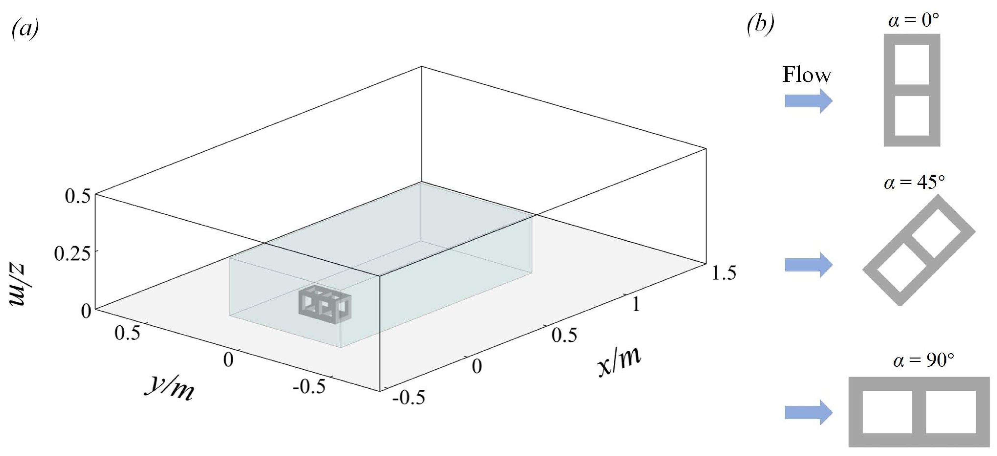
The computational domain is shown in Figure 2a, with and in the streamwise and spanwise directions, respectively. The wall-normal height of the domain () is 5H. The computational domain size is selected to minimize unnecessary computations, while the center is positioned 5.5L downstream of the inlet to ensure full flow development. A prescribed inflow condition is employed at the inlet of the domain. This is obtained by conducting simulations without the cuboid AR, using periodic boundary conditions. The instantaneous velocity at one cross section of the domain is saved for 5 flow-through periods () after the flow had fully developed and is then used as the inlet condition for all simulations. Convective boundary conditions are applied at the outlet of the domain, and periodic boundary conditions are imposed at the sidewalls. The no-slip boundary condition is applied at the bottom of the domain, while a free-slip boundary condition is used at the top of the domain. In order to investigate the effect of the angles () of inflow on the flow structure around the CAR, the placement angles () of the CAR are varied to 0°, 45°, and 90°, as shown in Figure 2b. Table 1 summarizes the flow conditions for three cases, including the inlet velocity (), water depth (h), and inflow angle ().

Figure 2.
(a) Sketch of the computational domain where the blue region represents the area of local mesh refinement and (b) the inflow with different angles (0°, 45°, and 90°).

Table 1.
Detailed flow conditions of the analyzed cases.
The computational mesh is refined through two levels of local mesh refinement, as illustrated in Figure 2a, with a finer resolution grid set in the vicinity of the CAR (−0.35 m < x < 0.95 m, −0.3 m < y < 0.3 m, 0 m < z < 0.25 m). Two different grid resolutions are selected for the analysis of grid sensitivity, and the sizes of the mesh are listed in Table 2. For Mesh 1, there are a total of approximately 8.94 million grid points. The finer grid resolution (Mesh 2) was discretized with 55.75 million computational points. All simulations are run for 10 to obtain the fully developed flow after the prescribed inflow imposed at the inlet. First-order statistics are collected after an additional 10 , and second-order statistics commence after a further 20 .
Table 2.
Grid resolutions used for grid sensitivity analysis.
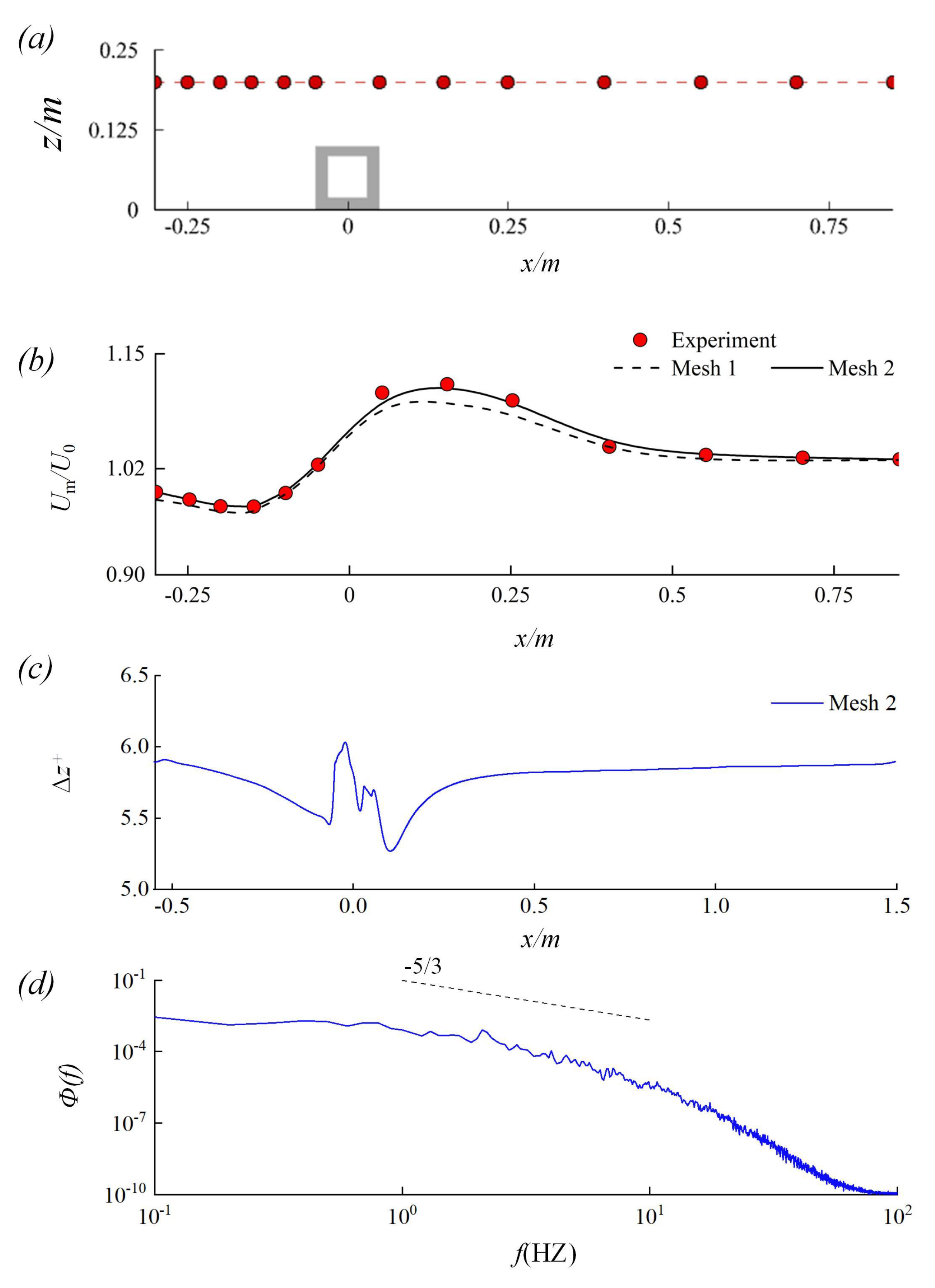
Figure 3a illustrates the locations of the validation points used in the experiment, while Figure 3b shows the profile of the normalized time-averaged streamwise velocity, comparing the results from the two LES simulations with the experimental data. Overall, a satisfying match is observed between the LES results and experimental data. The normalized streamwise velocity (/) experiences a slight decline before gradually increasing from x = −0.15 m, peaking at approximately x = 0.15 m, and then slowly decreasing to 1.02. The results from Mesh 1 (dashed line) show slight discrepancies, particularly in the range m, probably due to insufficient resolution. These discrepancies are reduced in the results from a finer mesh (Mesh 2). The wall-normal distance of the first computational point () along the length of the computational domain is presented in Figure 3c. The average value along the streamwise direction is approximately = 5.78, which is less than 12 [47], indicating that the near-wall grids remain within the viscous sublayer and ensuring that the simulations are wall resolved. A sampling point downstream of the CAR is chosen, and the time series of the instantaneous velocity data are recorded. The power spectral density (PSD) of the velocity fluctuations at this point is shown in Figure 3d. The results indicate that the energy cascade along the inertial subrange follows the −5/3 Kolmogorov law, indicating a physically realistic energy transfer between scales. An increased dissipation rate is found at higher frequencies due to the sub-grid scale model. Therefore, the resolution of Mesh 2 is chosen to conduct the subsequent simulations.
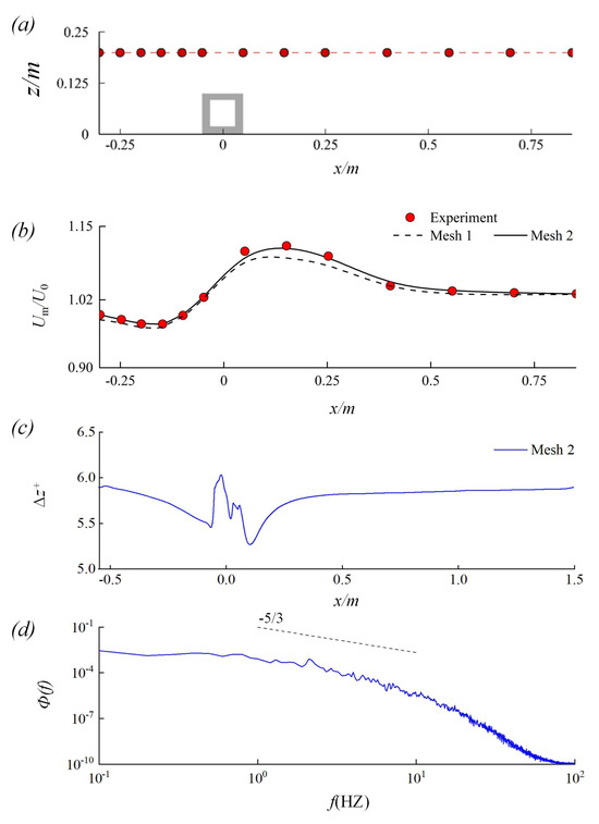
Figure 3.
(a) Locations of the validation points, (b) validation between LES and experiment, (c) the wall-normal grid spacing of the simulation, and (d) power spectral density of the velocity fluctuation at the sampling point.
3. Results and Discussions
3.1. Time-Averaged Flow and Flow Separation
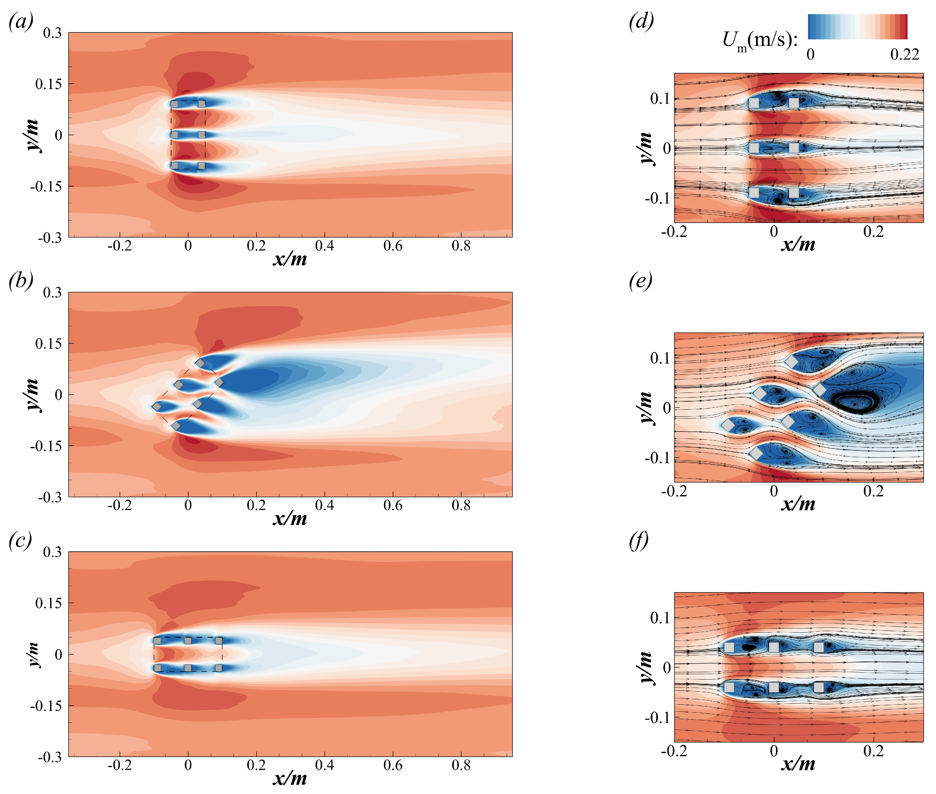
Figure 4 presents the contours of the time-averaged velocity distribution (left) and streamlines (right) at the plane for the three cases. The presence of the CAR notably alters the incoming flow, creating distinct low-velocity and high-velocity zones due to the blockage effect of the CAR. As shown in Figure 4a, high-velocity zones are located on either side of the CAR, with the maximum velocity () reaching approximately 0.228 m/s. In Case 2 and Case 3, is approximately 0.224 m/s and 0.205 m/s, respectively. Case 3 exhibits the lowest , which can be attributed to the weakest blockage effect among the three cases. The low-velocity zones, indicated by the blue regions in Figure 4a–c, exhibit significant variations in both extent and intensity. These zones are observed behind the square cylinders of the CAR due to the sheltering effect. In Case 1 and Case 3 ( = 0° or 90°), the development of the low-velocity zones is relatively limited, especially in the transverse direction. In contrast, the distribution of low-velocity zones in Case 2 ( = 45°) shows considerable differences, in both the streamwise and transverse directions. Additionally, the minimum velocities () in Case 1 and Case 3 are −0.0233 m/s and −0.0236 m/s, respectively, while in Case 2, drops to −0.0562 m/s.

Figure 4.
Contours of the time-averaged velocity distribution (left) and streamlines (right) at the plane : (a,d) for the case with ; (b,e) for the case with ; (c,f) for the case with .
In order to highlight flow separation and recirculation, the two-dimensional (2D) streamlines together with the contours of velocity are plotted in Figure 4d–f. Several recirculation zones occur downstream of these square cylinders, consistent with the studies previously reported by Liu et al. and Zheng et al. [11,48]. In Case 1, the maximum length of the recirculation zone is approximately 0.055 m, located at the center of the CAR. lt is interesting to note that the sizes of the recirculation bubble in Case 2 increase dramatically. More specifically, the maximum length of the recirculation bubble in Case 2 ( = 45°) is approximately 0.139 m, which is approximately 2.5 times that of Case 1. In Case 3, the characteristics of the recirculation zones are similar to those in Case 1, with the maximum length of the recirculation zone being approximately 0.0478 m, slightly smaller than that of Case 1.
Both the time-averaged velocity distribution and streamline plots indicate that the case with an inflow angle of 45° demonstrates the best performance, as it results in the largest low-velocity and recirculation zones. This is attributed to the fact that when the inflow angle equals 45°, it allows for the largest area of incoming flow, leading to the formation of a larger deceleration area in front of and inside the CAR.
3.2. Turbulence Parameters
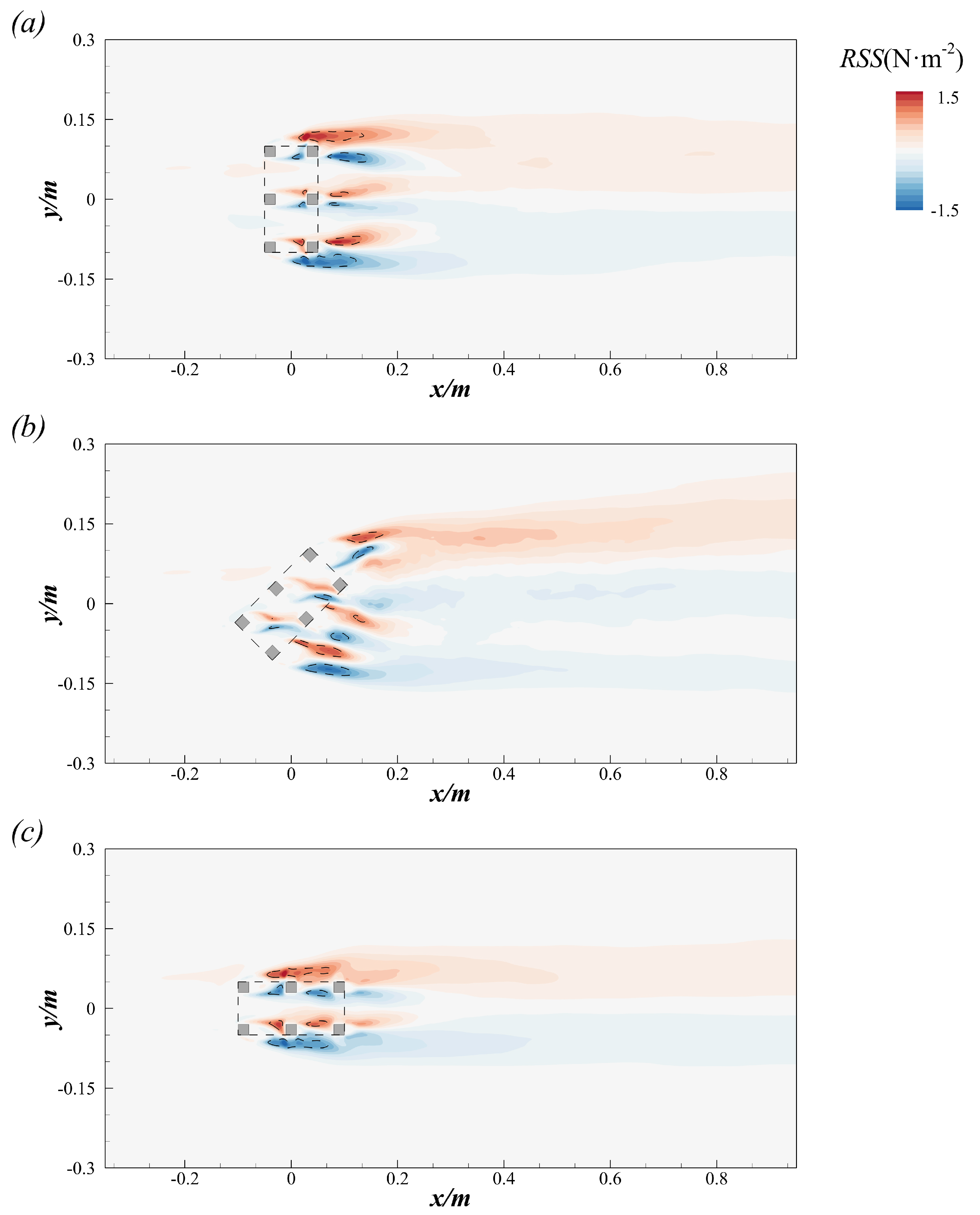
Figure 5 compares the distribution of the Reynolds shear stress (), calculated as , at = 0.5 across the three cases, highlighting the spatial distribution of turbulence within these cross sections. High-level regions are primarily observed inside and downstream of the CAR in all simulations, where the velocity gradients are most pronounced. In Case 1, the high-level regions originate from the location at and develop downstream, as shown in Figure 5a. The regions where N/m2 are highlighted by dashed lines, and these areas are primarily concentrated on both sides of the CAR. Peaks in occur on both sides of the CAR, with a maximum value of N/m2. The distribution of at the same plane of the inflow angle () equal to 45° is presented in Figure 5b. The region of high remains visible downstream of the CAR; however, it expands both streamwise and spanwise. The maximum value of in Case 2 is ≈ N/m2, which is slightly lower than that in Case 1. The distribution of in Case 3 shows symmetry along , similar to that in Case 1, as depicted in Figure 5c. Notably, the region where N/m2 is observed only inside and on the sides of the CAR, with a peak value of approximately N/m2.
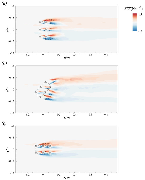
Figure 5.
Contours of the Reynolds shear stress at the plane : (a) for the case with ; (b) for the case with ; (c) for the case with .
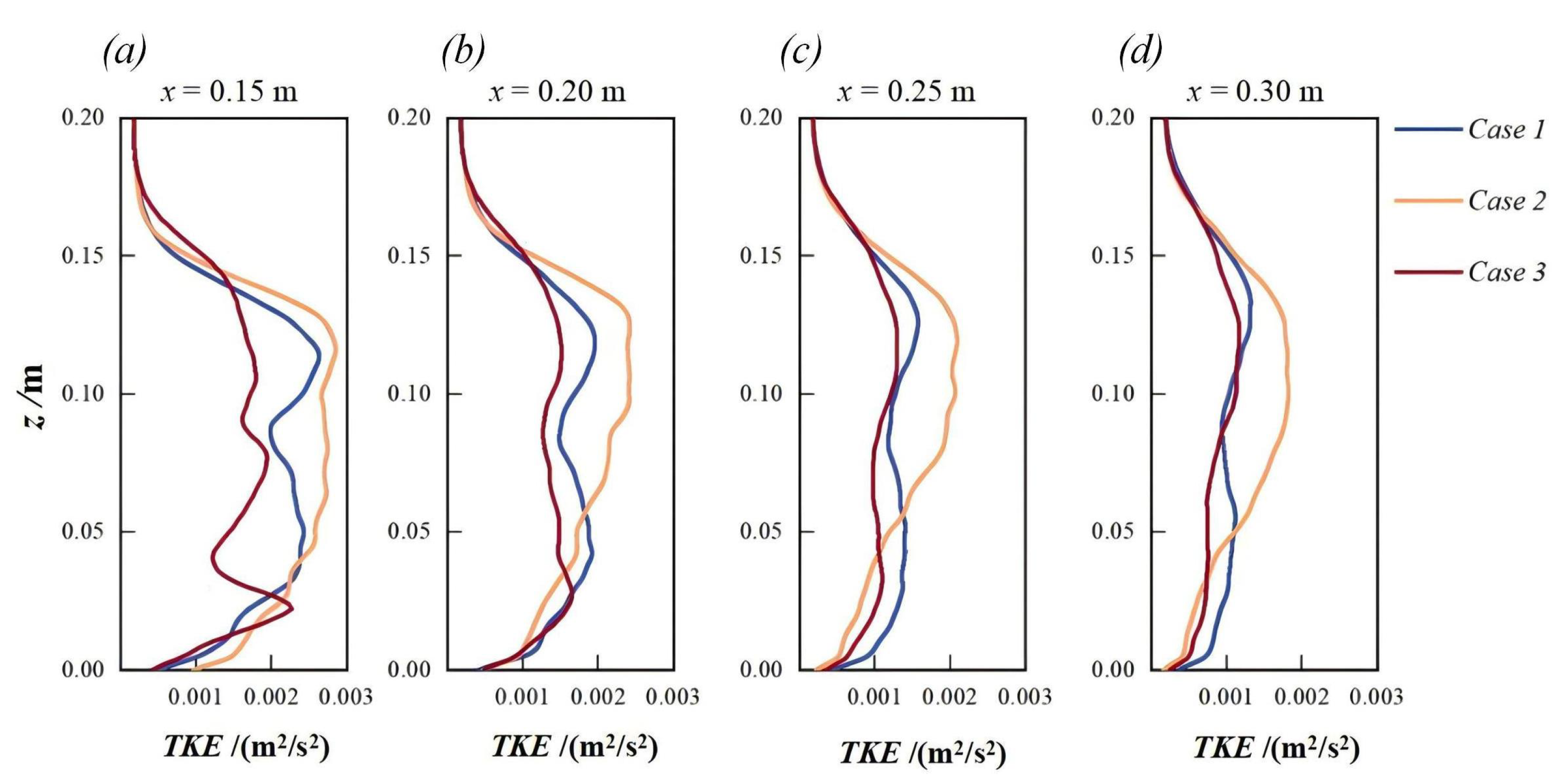
Vertical profiles of turbulent kinetic energy ()) at four locations downstream at the plane are presented in Figure 6 for the three simulated cases. In Case 1 and Case 3, a local peak value of can be observed in the curves. More specifically, the profiles of exhibit multiple peaks at m, m, and m. This is attributed to the shear layer at the corresponding location. For Case 1, the peak value of occurs approximately at m due to the shear layer near the upper side of the CAR. A clear peak could not be identified in Case 3 with an inflow angle (), as shown in Figure 6a. Further downstream, local peaks become less pronounced due to the weakening of the shear layer, as depicted in Figure 6b–d. Notably, Case 2 exhibits a higher level of compared with Case 1 and Case 3 at most locations. For example, 0.3 m downstream of the CAR, the values at m are 0.00104, 0.00182, and 0.00113 m2/s2 for Case 1, Case 2, and Case 3, respectively, as shown in Figure 6d.

Figure 6.
Vertical profiles of turbulent kinetic energy at four locations downstream of the CAR at the plane : (a) for m, (b) for m, (c) for m, and (d) for m.
The turbulent dynamics around ARs are crucial, as they significantly influence the mixing and transport of nutrients within the surrounding area [48]. Moreover, and are critical metrics for assessing the impact of turbulence on fish behavior [49,50]. High-levels of or can lead to disorientation or even physical harm to fish [51]. In turbulent environments, thresholds of < 10 N/m2 and < 0.5 m2/s2 are typically considered favorable for fish species [52]. Consequently, the design and placement of ARs should carefully account for both factors.
3.3. Instantaneous Flow Structures
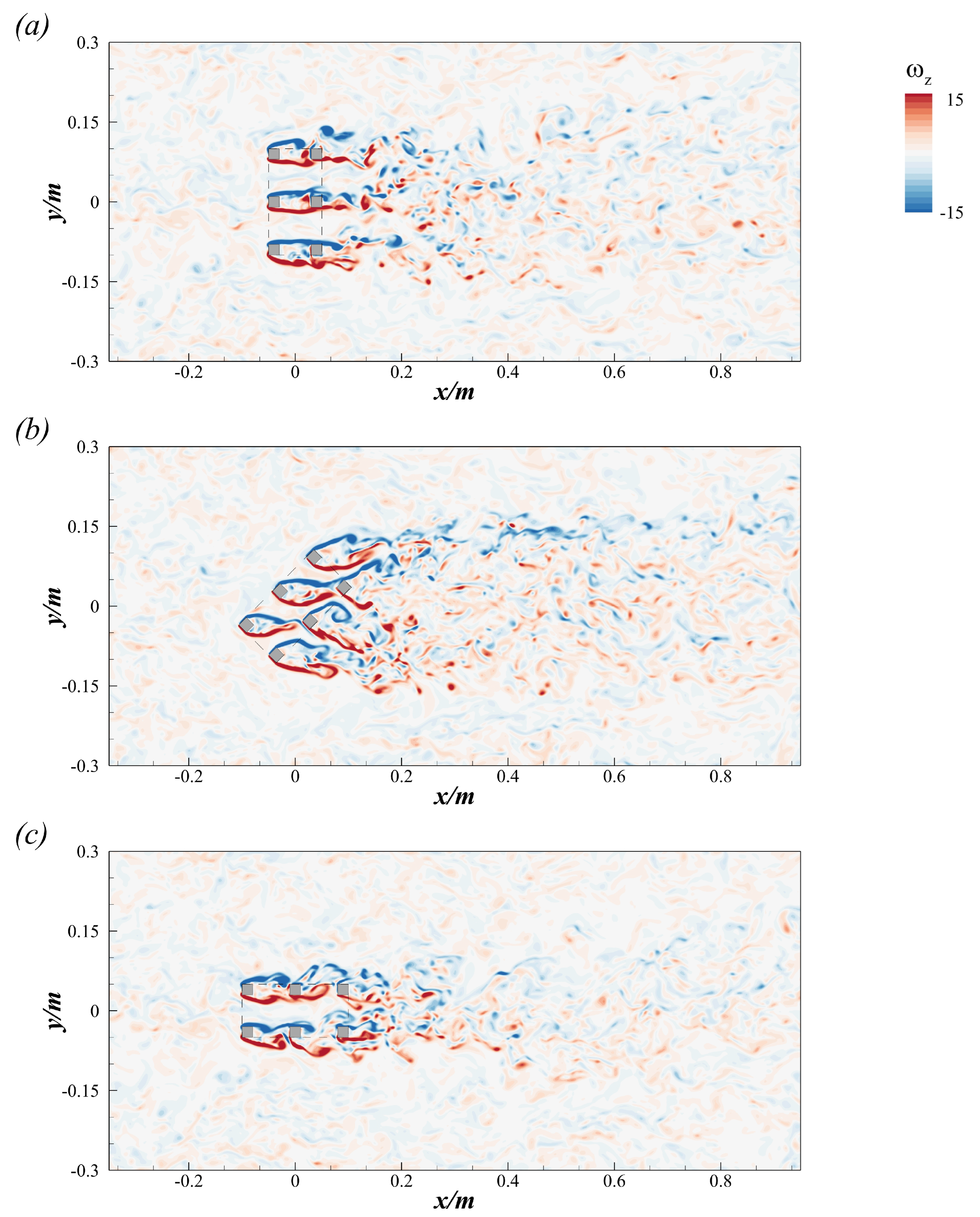
The flow through and around the CAR exhibits strong three-dimensional characteristics and is primarily influenced by different scales of turbulent structures, whose configuration is largely determined by the angle of inflow. Figure 7 presents contours of instantaneous vertical vorticity () at the plane at varying inflow angles. This plot illustrates the formation of the shear layer around the CAR. In Case 1, the shear layer separates from the leading edge of the upstream square cylinder, wraps around the downstream square cylinder, and continues to develop further downstream. This flow pattern resembles the flow around two cylinders arranged in tandem [53]. The vortex in the wake region downstream of the CAR gradually dissipates, following a pattern similar to a classic von Kármán vortex street. As the inflow angle varies from to , the development of the shear layer changes. Part of the shear layer separates and moves directly downstream, while another portion detaches and evolves through the gap between the square cylinders inside the CAR. It is interesting to note that the wake vortex expands spanwise while moving downstream due to more significant shear deformation inside the CAR, as shown in Figure 7b. In the case of , the spanwise development of the vortex is significantly restricted, confined to the range of m m, where the CAR obstructs the main flow (Figure 7c).

Figure 7.
Contours of instantaneous vertical vorticity () at the plane : (a) for the case with ; (b) for the case with ; (c) for the case with .
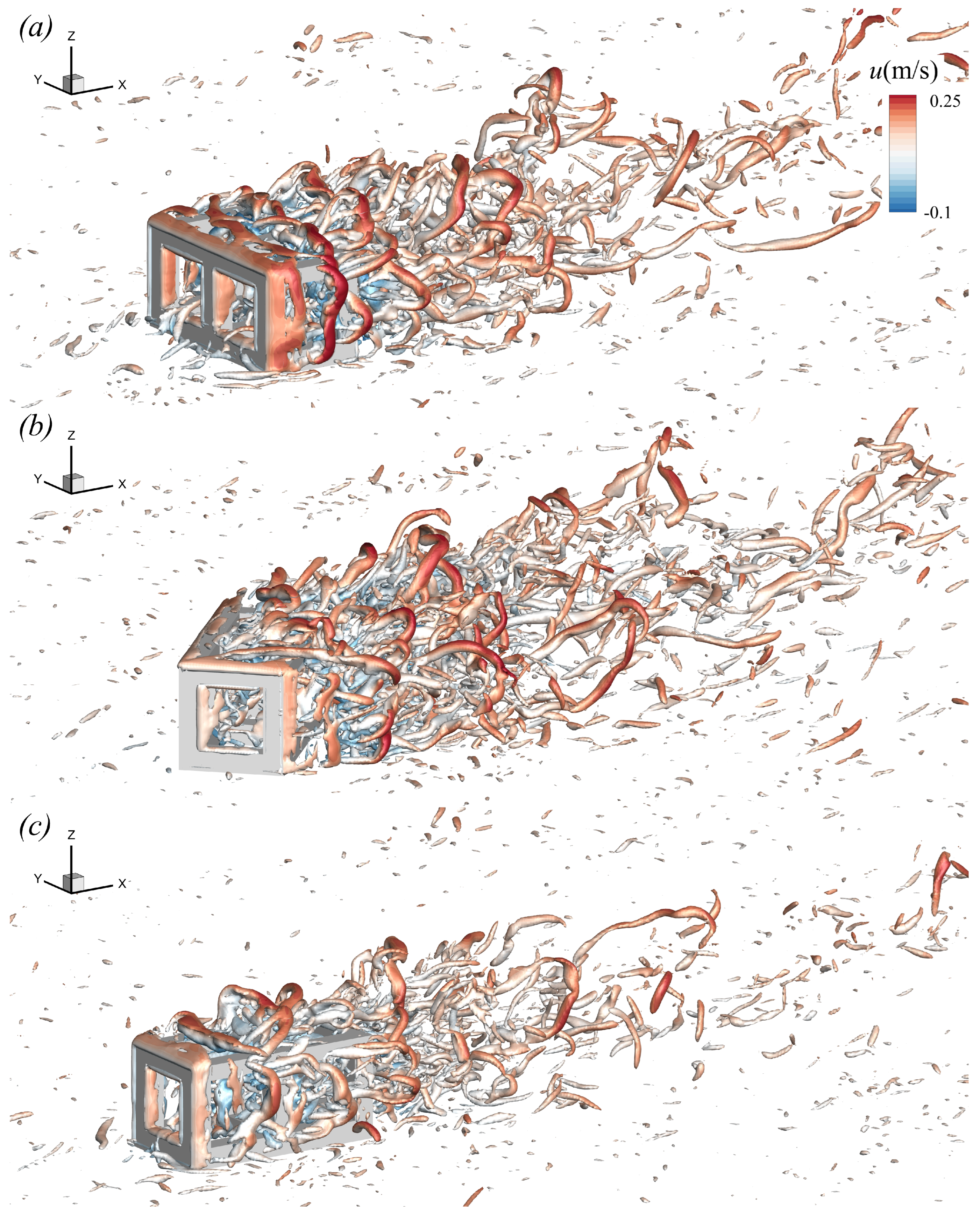
To better visualize the 3D turbulent structures around the CAR, the Q criterion method, a second-generation vortex identification technique, is used. Figure 8 presents the the isosurfaces of the Q-criterion, contoured with instantaneous streamwise velocity (u) for three different inflow angles ( = 0°, 45°, and 90°). Different types of the turbulence structures can be classified. A spanwise roller is found shed from the upper side of the CAR, i.e., quasi-2D structures that rotate about the y-axis (Figure 8a). The roller subsequently forms a hairpin vortex and is transported downstream by the main current. Similar rollers are also found on the sides of the CAR, where they subsequently evolve into vertical vortices. The formation of these rollers is driven by flow separation and the roll-up of the shear layer. Unlike the flow around typical bluff bodies, such as a cube [54], a complete horseshoe vortex cannot be identified in front of the CAR. Instead, only the legs of torn horseshoe vortices are observed through the gap inside the CAR. Similarly, the aforementioned vortex structures are also found in the cases of = 45° and 90°, as shown in Figure 8b,c. The main differences lie in the length, scale, and direction of these vortices.

Figure 8.
Isosurfaces of Q criterion for three cases, colored with instantaneous streamwise velocity: (a) for the case with ; (b) for the case with ; (c) for the case with .
3.4. Upwelling and Wake Region Parameters
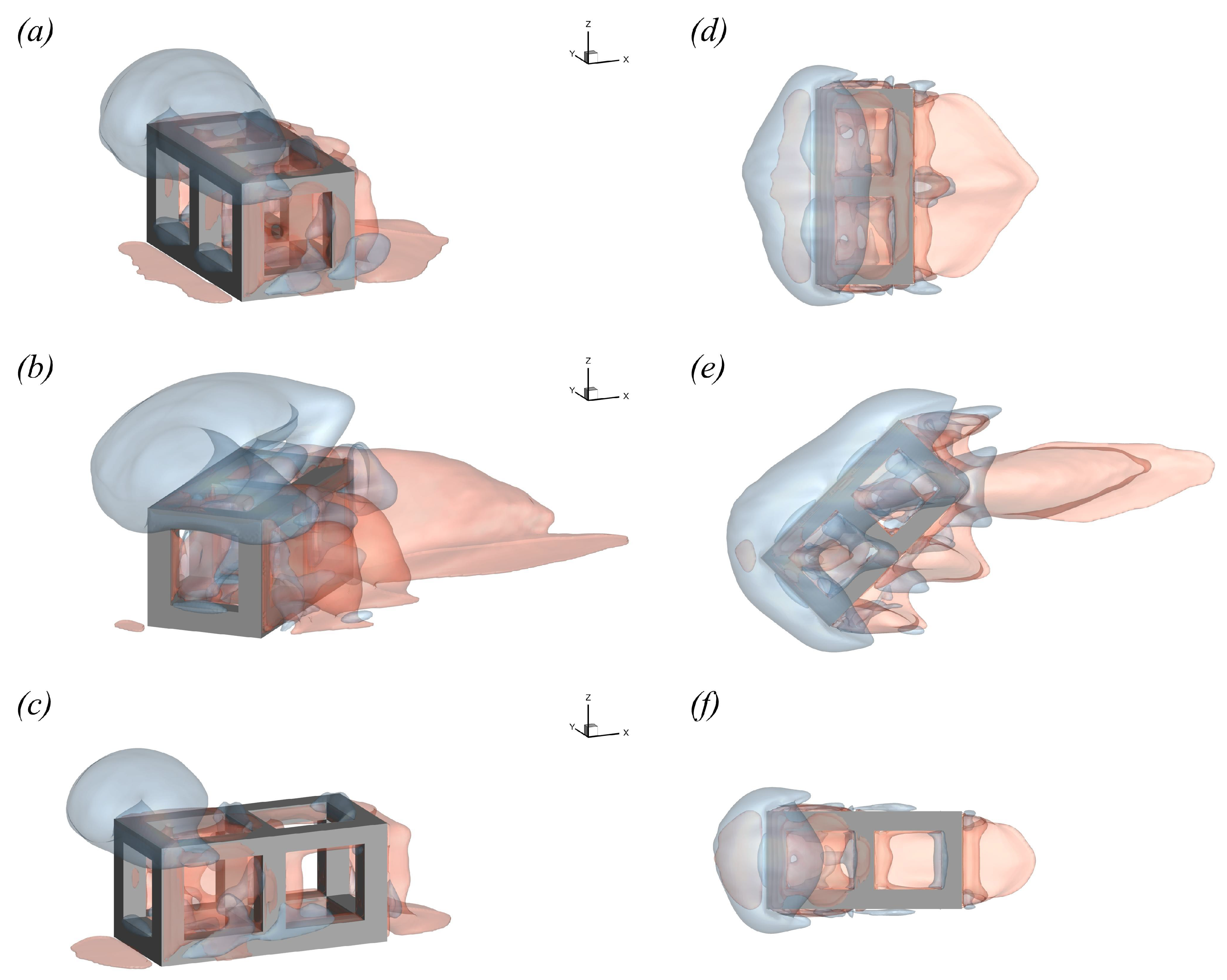
To quantify the effect of inflow angles (0°, 45°, and 90°) on the upwelling and wake regions, the isosurfaces of these regions are plotted in Figure 9. The upwelling region is indicated by the blue area in Figure 9a, mainly occurring on the upper front of the CAR. This is attributed to the blocking effect of the CAR, leading to the flow lifting and moving around. The wake region mainly exists downstream of the CAR, where flow separation occurs.The distribution of the upwelling and wake regions is almost symmetrical along the centerline of the CAR, as shown in Figure 9d. As the inflow angle increases, the characteristics of the upwelling and wake regions change significantly, in both size and shape, as depicted in Figure 9b,e. The upwelling region nearly covers the full extent of both the streamwise and spanwise of the CAR. At the same time, part of the wake region extends further downstream. In Case 3 ( = 90°), the size of these two regions decreases significantly, as depicted in Figure 9c,f.

Figure 9.
Side view (left) and top view (right) of distribution of the upwelling and wake region: (a,d) for the case with ; (b,e) for the case with ; (c,f) for the case with .
The volumes of the upwelling () and wake region () are summarized in Table 3. As shown in Table 3, Case 2, with an inflow angle of , exhibits the largest volumes of both the upwelling and wake regions compared with Cases 1 and 3 ( m3 and m3). and in Case 1 decrease by approximately 35% and 15%, respectively, compared with Case 2. As expected, Case 3 () exhibits the smallest volumes for both the upwelling and wake regions, with m3 and m3, showing a decrease of approximately 64% and 21%, respectively, compared with Case 2.
Table 3.
Volumes of the upwelling () and wake region ().
4. Conclusions
The present study has investigated the flow field around a cuboid artificial reef (CAR) with three inflow angles ( = 0°, 45°, and 90°), utilizing the open-source large eddy simulation (LES) code. First, the LES has been validated with the velocity data in the experiment, and a good agreement has been obtained. It examines variations of inflow angles on hydrodynamics and turbulence structures around the CAR. Key findings from this study include the following:
- (1)
- Time-averaged velocity distribution and streamline plots indicated that flow separation occurs inside and downstream of the CAR. Case 2 has the maximum length of the recirculation bubble, 2.5 times and 2.9 times greater than that of Case 1 and Case 3, respectively.
- (2)
- The high-level region of the Reynolds shear stress () is located where flow separation occurs. This region extends the most in both the streamwise and spanwise directions when the inflow angle is 45°. Additionally, Case 2 exhibits higher levels of turbulence kinetic energy () compared with Case 1 and Case 3 at most vertical locations downstream of the CAR.
- (3)
- The instantaneous flow around the CAR is characterized by significant shear layers prevailing from the leading edge of square cylinders. Isosurfaces of the Q-criterion reveal various types of turbulent structures, including torn horseshoe vortices and hairpin vortices, with the latter formed from the rollers shed by the shear layer.
- (4)
- Case 2, with an inflow angle of , exhibits the largest volumes for both the upwelling and wake regions. Compared with Case 2, and in Case 1 () decrease by approximately 35% and 15%, respectively. Case 3 () shows the smallest volumes for both regions, with reductions of approximately 64% and 21% for and , respectively, compared with Case 2.
Author Contributions
Conceptualization, J.D., Q.X. and J.M.; methodology, J.D., Q.X. and Y.G.; formal analysis, Y.L. and X.L.; writing—original draft preparation, J.D., Y.G. and Y.L.; writing—review and editing, X.L. and J.M.; visualization, J.D., Q.X. and Y.L.; supervision, X.L. and J.M.; project administration, X.L. and J.M. All authors have read and agreed to the published version of the manuscript.
Funding
This work was supported by the National Key Research and Development Program of China (2023YFC3209200), Hubei Provincial Natural Science Foundation of China (2023AFD201), and National Natural Science Foundation of China (52279013, 52279055, and U2040205).
Institutional Review Board Statement
Not applicable.
Informed Consent Statement
Not applicable.
Data Availability Statement
Data can be obtained from the first author upon request.
Acknowledgments
The authors gratefully acknowledge the support from the fundings listed above. We also appreciate the anonymous reviewers who gave comments to revise the paper.
Conflicts of Interest
Author Qianshun Xu was employed by the company Yellow River Engineering Consulting Co., Ltd., and author Xinbo Liu was employed by the company China Yangtze Power Co., Ltd. The remaining authors declare that the research was conducted in the absence of any commercial or financial relationships that could be construed as potential conflicts of interest.
References
- Au, D. The application of histo-cytopathological biomarkers in marine pollution monitoring: A review. Mar. Pollut. Bull. 2004, 48, 817–834. [Google Scholar] [CrossRef] [PubMed]
- Hoegh-Guldberg, O. Coral reef ecosystems and anthropogenic climate change. Reg. Environ. Change 2011, 11, 215–227. [Google Scholar] [CrossRef]
- Wu, W.; Yang, Z.; Tian, B.; Huang, Y.; Zhou, Y.; Zhang, T. Impacts of coastal reclamation on wetlands: Loss, resilience, and sustainable management. Estuar. Coast. Shelf Sci. 2018, 210, 153–161. [Google Scholar] [CrossRef]
- Guo, X.; Fan, N.; Zheng, D.; Fu, C.; Wu, H.; Zhang, Y.; Song, X.; Nian, T. Predicting impact forces on pipelines from deep-sea fluidized slides: A comprehensive review of key factors. Int. J. Mining Sci. Technol. 2024, 34, 211–225. [Google Scholar] [CrossRef]
- Lee, M.O.; Otake, S.; Kim, J.K. Transition of artificial reefs (ARs) research and its prospects. Ocean Coast. Manag. 2018, 154, 55–65. [Google Scholar] [CrossRef]
- Lima, J.S.; Zalmon, I.R.; Love, M. Overview and trends of ecological and socioeconomic research on artificial reefs. Mar. Environ. Res. 2019, 145, 81–96. [Google Scholar] [CrossRef]
- Bull, A.S.; Love, M.S. Worldwide oil and gas platform decommissioning: A review of practices and reefing options. Ocean Coast. Manag. 2019, 168, 274–306. [Google Scholar] [CrossRef]
- Simon, T.; Pinheiro, H.T.; Joyeux, J.C. Target fishes on artificial reefs: Evidences of impacts over nearby natural environments. Sci. Total Environ. 2011, 409, 4579–4584. [Google Scholar] [CrossRef] [PubMed]
- Walles, B.; Troost, K.; van den Ende, D.; Nieuwhof, S.; Smaal, A.C.; Ysebaert, T. From artificial structures to self-sustaining oyster reefs. J. Sea Res. 2016, 108, 1–9. [Google Scholar] [CrossRef]
- Paxton, A.B.; Peterson, C.H.; Taylor, J.C.; Adler, A.M.; Pickering, E.A.; Silliman, B.R. Artificial reefs facilitate tropical fish at their range edge. Commun. Biol. 2019, 2, 168. [Google Scholar] [CrossRef] [PubMed]
- Liu, T.L.; Su, D.T. Numerical analysis of the influence of reef arrangements on artificial reef flow fields. Ocean Eng. 2013, 74, 81–89. [Google Scholar] [CrossRef]
- Kim, D.; Woo, J.; Na, W.B. Intensively stacked placement models of artificial reef sets characterized by wake and upwelling regions. Mar. Technol. Soc. J. 2017, 51, 60–70. [Google Scholar] [CrossRef]
- Santiago Caamaño, L.; Lamas Galdo, M.I.; Carballo, R.; López, I.; Cartelle Barros, J.J.; Carral, L. Numerical and experimental analysis of the velocity field inside an artificial reef. Application to the Ares-Betanzos estuary. J. Mar. Sci. Eng. 2022, 10, 1827. [Google Scholar] [CrossRef]
- Liu, Y.; Zhao, Y.P.; Dong, G.H.; Guan, C.T.; Cui, Y.; Xu, T.J. A study of the flow field characteristics around star-shaped artificial reefs. J. Fluids Struct. 2013, 39, 27–40. [Google Scholar] [CrossRef]
- Jiao, L.; Yan-Xuan, Z.; Pi-Hai, G.; Chang-Tao, G. Numerical simulation and PIV experimental study of the effect of flow fields around tube artificial reefs. Ocean Eng. 2017, 134, 96–104. [Google Scholar] [CrossRef]
- Wu, J.; Zhang, S.; Sun, M.; Chen, Y. Experiment on the distribution of different artificial reef models for Paralichthys olivaceus. Mar. Fish. 2004, 26, 394–398. [Google Scholar]
- Kim, D.; Woo, J.; Yoon, H.S.; Na, W.B. Efficiency, tranquillity and stability indices to evaluate performance in the artificial reef wake region. Ocean Eng. 2016, 122, 253–261. [Google Scholar] [CrossRef]
- Wang, X.; Liu, X.; Tang, Y.; Zhao, F.; Luo, Y. Numerical analysis of the flow effect of the menger-type artificial reefs with different void space complexity indices. Symmetry 2021, 13, 1040. [Google Scholar] [CrossRef]
- Kim, D.; Woo, J.; Yoon, H.S.; Na, W.B. Wake lengths and structural responses of Korean general artificial reefs. Ocean Eng. 2014, 92, 83–91. [Google Scholar] [CrossRef]
- Maslov, D.; Pereira, E.; Duarte, D.; Miranda, T.; Ferreira, V.; Tieppo, M.; Cruz, F.; Johnson, J. Numerical analysis of the flow field and cross section design implications in a multifunctional artificial reef. Ocean Eng. 2023, 272, 113817. [Google Scholar] [CrossRef]
- Shu, A.; Qin, J.; Rubinato, M.; Sun, T.; Wang, M.; Wang, S.; Wang, L.; Zhu, J.; Zhu, F. An experimental investigation of turbulence features induced by typical artificial M-shaped unit reefs. Appl. Sci. 2021, 11, 1393. [Google Scholar] [CrossRef]
- Jiang, Z.; Liang, Z.; Zhu, L.; Liu, Y. Numerical simulation of effect of guide plate on flow field of artificial reef. Ocean Eng. 2016, 116, 236–241. [Google Scholar] [CrossRef]
- Liao, J.C. A review of fish swimming mechanics and behaviour in altered flows. Philos. Trans. R. Soc. B Biol. Sci. 2007, 362, 1973–1993. [Google Scholar] [CrossRef]
- Fang, H.; Liu, Y.; Stoesser, T. Influence of boulder concentration on turbulence and sediment transport in open-channel flow over submerged boulders. J. Geophys. Res. Earth Surf. 2017, 122, 2392–2410. [Google Scholar] [CrossRef]
- Muhawenimana, V.; Wilson, C.; Ouro, P.; Cable, J. Spanwise cylinder wake hydrodynamics and fish behavior. Water Resour. Res. 2019, 55, 8569–8582. [Google Scholar] [CrossRef]
- Yusuf, S.N.A.; Asako, Y.; Sidik, N.A.C.; Mohamed, S.B.; Japar, W.M.A.A. A short review on rans turbulence models. CFD Lett. 2020, 12, 83–96. [Google Scholar]
- Zhao, C.; Ouro, P.; Stoesser, T.; Dey, S.; Fang, H. Response of flow and saltating particle characteristics to bed roughness and particle spatial density. Water Resour. Res. 2022, 58, e2021WR030847. [Google Scholar] [CrossRef]
- Jiang, Z.; Liang, Z.; Liu, Y.; Tang, Y.; Huang, L. Particle image velocimetry and numerical simulations of the hydrodynamic characteristics of an artificial reef. Chin. J. Oceanol. Limnol. 2013, 31, 949–956. [Google Scholar] [CrossRef]
- Kim, D.; Woo, J.; Na, W.B.; Yoon, H.S. Flow and structural response characteristics of a box-type artificial reef. J. Korean Soc. Coast. Ocean Eng. 2014, 26, 113–119. [Google Scholar] [CrossRef]
- Kim, D.; Jung, S.; Na, W.B. Evaluation of turbulence models for estimating the wake region of artificial reefs using particle image velocimetry and computational fluid dynamics. Ocean Eng. 2021, 223, 108673. [Google Scholar] [CrossRef]
- Jalalabadi, R.; Stoesser, T.; Ouro, P.; Luo, Q.; Xie, Z. Free surface flow over square bars at different Reynolds numbers. J. Hydro-Environ. Res. 2021, 36, 67–76. [Google Scholar] [CrossRef]
- He, K.; Su, X.; Gao, G.; Krajnović, S. Evaluation of LES, IDDES and URANS for prediction of flow around a streamlined high-speed train. J. Wind Eng. Ind. Aerodyn. 2022, 223, 104952. [Google Scholar] [CrossRef]
- Sheidani, A.; Salavatidezfouli, S.; Stabile, G.; Rozza, G. Assessment of URANS and LES methods in predicting wake shed behind a vertical axis wind turbine. J. Wind Eng. Ind. Aerodyn. 2023, 232, 105285. [Google Scholar] [CrossRef]
- Ouro, P.; Juez, C.; Franca, M. Drivers for mass and momentum exchange between the main channel and river bank lateral cavities. Adv. Water Resour. 2020, 137, 103511. [Google Scholar] [CrossRef]
- Luo, Q.; Dolcetti, G.; Stoesser, T.; Tait, S. Water surface response to turbulent flow over a backward-facing step. J. Fluid Mech. 2023, 966, A18. [Google Scholar] [CrossRef]
- Guo, X.; Luo, Q.; Stoesser, T.; Hajaali, A.; Liu, X. Evolution of high-density submarine turbidity current and its interaction with a pair of parallel suspended pipes. Phys. Fluids 2023, 35, 086608. [Google Scholar] [CrossRef]
- Liu, Y.; Stoesser, T.; Fang, H.; Papanicolaou, A.; Tsakiris, A.G. Turbulent flow over an array of boulders placed on a rough, permeable bed. Comput. Fluids 2017, 158, 120–132. [Google Scholar] [CrossRef]
- Alzabari, F.; Wilson, C.A.; Ouro, P. Hydrodynamics of in-stream leaky barriers for natural flood management. Water Resour. Res. 2024, 60, e2024WR038117. [Google Scholar] [CrossRef]
- Guo, X.; Liu, X.; Zheng, T.; Zhang, H.; Lu, Y.; Li, T. A mass transfer-based LES modelling methodology for analyzing the movement of submarine sediment flows with extensive shear behavior. Coastal Eng. 2024, 191, 104531. [Google Scholar] [CrossRef]
- Zhang, J.; Zhu, L.; Liang, Z.; Sun, L.; Nie, Z.; Wang, J.; Xie, W.; Jiang, Z. Numerical study of efficiency indices to evaluate the effect of layout mode of artificial reef unit on flow field. J. Mar. Sci. Eng. 2021, 9, 770. [Google Scholar] [CrossRef]
- Gong, Y.; Stoesser, T.; Mao, J.; McSherry, R. LES of flow through and around a finite patch of thin plates. Water Resour. Res. 2019, 55, 7587–7605. [Google Scholar] [CrossRef]
- Luo, Q.; Stoesser, T.; Cameron, S.; Nikora, V.; Zampiron, A.; Patella, W. Meandering of instantaneous large-scale structures in open-channel flow over longitudinal ridges. Environ. Fluid Mech. 2023, 23, 829–846. [Google Scholar] [CrossRef]
- Liu, Y.; Tang, Z.; Huang, L.; Stoesser, T.; Fang, H. On the role of the Froude number on flow, turbulence, and hyporheic exchange in open-channel flow through boulder arrays. Phys. Fluids 2024, 36, 095141. [Google Scholar] [CrossRef]
- Dai, J.; Mao, J.q.; Gong, Y.Q.; Gao, H. Effect of triangular baffle designs on flow dynamics and sediment transport within standard box culverts. J. Hydrodyn. 2025, 1–13. [Google Scholar] [CrossRef]
- Nicoud, F.; Ducros, F. Subgrid-scale stress modelling based on the square of the velocity gradient tensor. Flow Turbul. Combust. 1999, 62, 183–200. [Google Scholar] [CrossRef]
- Tan, S.f.; Wang, X.z.; Zhang, M.; Liu, C.g.; Wang, A.m.; Xu, X.f.; Xu, P. Flow field effect of cuboid frame artificial reef. Chin. J. Appl. Mech. 2025. online first (In Chinese) [Google Scholar]
- Rodi, W.; Constantinescu, G.; Stoesser, T. Large-Eddy Simulation in Hydraulics; CRC Press: Boca Raton, FL, USA, 2013. [Google Scholar]
- Zheng, Y.; Kuang, C.; Zhang, J.; Gu, J.; Chen, K.; Liu, X. Current and turbulence characteristics of perforated box-type artificial reefs in a constant water depth. Ocean Eng. 2022, 244, 110359. [Google Scholar] [CrossRef]
- Farzadkhoo, M.; Kingsford, R.T.; Suthers, I.M.; Felder, S. Flow hydrodynamics drive effective fish attraction behaviour into slotted fishway entrances. J. Hydrodyn. 2023, 35, 782–802. [Google Scholar] [CrossRef]
- Wu, Y.; Liu, G.; Yang, J.; Xu, J.; Ke, S.; Li, D.; Chen, X.; Shi, X.; Lin, C. Avoidance behavior of grass carp (Ctenopharyngodon idella) shoals to low-frequency sound stimulation. Aquat. Sci. 2025, 87, 21. [Google Scholar] [CrossRef]
- Marriner, B.A.; Baki, A.B.; Zhu, D.Z.; Cooke, S.J.; Katopodis, C. The hydraulics of a vertical slot fishway: A case study on the multi-species Vianney-Legendre fishway in Quebec, Canada. Ecol. Eng. 2016, 90, 190–202. [Google Scholar] [CrossRef]
- Quaranta, E.; Katopodis, C.; Revelli, R.; Comoglio, C. Turbulent flow field comparison and related suitability for fish passage of a standard and a simplified low-gradient vertical slot fishway. River Res. Appl. 2017, 33, 1295–1305. [Google Scholar] [CrossRef]
- Palau-Salvador, G.; Stoesser, T.; Rodi, W. LES of the flow around two cylinders in tandem. J. Fluids Struct. 2008, 24, 1304–1312. [Google Scholar] [CrossRef]
- McSherry, R.J.; Chua, K.V.; Stoesser, T. Large eddy simulation of free-surface flows. J. Hydrodyn. Ser. B 2017, 29, 1–12. [Google Scholar] [CrossRef]
Disclaimer/Publisher’s Note: The statements, opinions and data contained in all publications are solely those of the individual author(s) and contributor(s) and not of MDPI and/or the editor(s). MDPI and/or the editor(s) disclaim responsibility for any injury to people or property resulting from any ideas, methods, instructions or products referred to in the content. |
© 2025 by the authors. Licensee MDPI, Basel, Switzerland. This article is an open access article distributed under the terms and conditions of the Creative Commons Attribution (CC BY) license (https://creativecommons.org/licenses/by/4.0/).