Article

Large-Eddy Simulation of Flows Past an Isolated Lateral Semi-Circular Cavity

1
Institute of Water Science and Technology, Hohai University, Nanjing 211106, China
2
Zhejiang Institute of Communications Co., Ltd., Hangzhou 310012, China
3
College of Water Conservancy and Hydropower Engineering, Hohai University, Nanjing 210098, China
4
College of Architectural Engineering, Zhejiang Tongji Vocational College of Science and Technology, Hangzhou 311231, China
5
Yellow River Engineering Consulting Co., Ltd., Zhengzhou 450003, China
*
Authors to whom correspondence should be addressed.
J. Mar. Sci. Eng. 2025, 13(5), 859; https://doi.org/10.3390/jmse13050859
Submission received: 27 March 2025 / Revised: 17 April 2025 / Accepted: 21 April 2025 / Published: 25 April 2025

Abstract

:
Lateral cavities along coastlines strongly influence sedimentary morphology and ecological processes by modifying local flow dynamics. This study employed high-resolution large-eddy simulation to investigate flow structures and momentum exchange mechanisms in a semi-circular lateral cavity driven by longshore currents. Model validation against experimental data confirmed the LES’s capability to capture both recirculating flow and turbulent structures accurately. The impact of Reynolds number was examined across three cases ( R e = 12,000, 17,000, and 22,000). From R e = 12,000 to 17,000, a significant upstream shift of the primary vortex core occurred, accompanied by stronger shear layer turbulence and intensified secondary vortices. Between R e = 17,000 and 22,000, the flow features stabilized, indicating a transition toward quasi-equilibrium. These changes enhanced vertical momentum transfer and turbulence production within the cavity. Spectral analysis revealed dominant KH frequencies governing periodic momentum exchange and indicating a transition from viscosity-damped upstream turbulence to fully developed shedding downstream.

1. Introduction

Coastal morphological evolution is governed by the interplay between hydrodynamic forces and sediment transport processes [1,2,3,4]. Among these, alongshore currents play a key role and are strongly influenced by shoreline geometry. Arc-shaped embayments and recessed features along the coast, which often result from morphological evolution, can significantly modify local hydrodynamics. These processes shape meandering shorelines and recessed morphological features that serve as critical zones for sediment retention and biodiversity enhancement [5,6]. Semi-enclosed natural cavities, such as bays and lagoons, facilitate vegetation colonization while providing essential fish nurseries [7,8]. Similarly, cuspate forelands and tombolos create localized embayments where flow attenuation promotes the selective deposition of fine sediments, reshaping coastal geomorphology and fostering niche habitats [9,10,11]. In estuarine systems, sinuous channel margins are often lined with lateral cavities that serve as brackish mixing zones and critical ecological transition corridors [12,13]. Lateral cavities enhance ecological resilience and support the long-term stability of coastal landscapes by promoting sedimentary self-organization and enabling hydrodynamic–biotic feedback. Artificial lateral cavities have also been adopted in nature-based coastal restoration strategies. In Sydney Harbour, localized cavity structures integrated into seawalls by Australian engineers have been shown to increase both the abundance and diversity of sessile species [14,15].
The ecological performance of natural and artificial cavities is tightly coupled to by their influence on local flow dynamics [16,17,18]. Mass transport and exchange across the cavity interface are governed by recirculating flow patterns, vortex shedding dynamics, and shear layer instabilities that develop within and around the cavities. Recent advances combining field observations, laboratory experiments, and numerical simulations have progressively clarified the fundamental physics of cavity flows, particularly the interdependent effects of Reynolds number ( R e ), aspect ratio, and morphological complexity on flow properties. An increase in R e typically results in a shift of the main vortex (MV) core, the emergence of additional counter-rotating corner vortices, and enhanced mass and momentum exchange across the cavity mouth [19,20,21]. The aspect ratio determines the spatial extent of the main recirculation zone and the threshold for secondary vortex formation [22,23,24]. Furthermore, topographic undulations and curved geometries further complicate the flow field by introducing an additional secondary corner and bottom vortices [25,26].
Despite significant progress in understanding cavity-induced hydrodynamics, most existing insights are derived from flow characteristics observed in fixed-spacing rectangular cavity arrays, such as groyne fields [27,28]. In these engineered multi-cavity systems, the shear layer originates at the leading edge of the first cavity, gradually develops downstream along the cavity–channel interface, and typically reaches a fully developed state by the fourth to sixth cavity [29,30]. Coherent vortical structures span the entire interface, facilitating a continuous momentum exchange across the cavity mouths. In contrast, natural coastal cavities differ fundamentally from such engineered configurations. They are discretely distributed with a significantly larger spacing, resulting in minimal upstream influence on downstream cavities under longshore currents. The upstream incoming boundary layer is different between the two cases: it is fully turbulent for continuous cavity arrays but remains laminar for an isolated cavity. Grace et al. [31] showed that a laminar incoming boundary layer produces a shear layer that remains stable near the cavity’s leading edge and gradually transitions to turbulence downstream, while a turbulent incoming boundary layer yields a shear layer that becomes fully turbulent immediately over the cavity opening.
A critical gap persists in the geometric representation of cavities. While the majority of existing studies have focused on orthogonal geometries (e.g., square or rectangular cavities) [32,33], natural lateral cavities predominantly exhibit curvilinear wetted perimeters [25,34]. However, the hydrodynamics of non-rectangular lateral cavities have received relatively limited attention. In particular, curved cavity geometries that arise from shoreline evolution and sedimentary processes—such as arc-shaped embayments, gullies, and wetland bays—are rarely isolated for detailed hydrodynamic investigations. Addressing this gap is essential for advancing our understanding of cavity–flow interactions and improving the predictive modeling of natural and engineered coastal systems. Some efforts have been made to examine shape effects. Ozalp et al. [35] experimentally investigated the influence of cavity shape on vortex formation, turbulence intensity, and flow entrainment. Their results showed that rectangular and triangular cavities generated stronger turbulence and more pronounced vortex structures compared to semi-circular cavities. Jackson et al. [36] further examined the effect of semi-circular cavity deformation on mean residence time, reporting that forward-conic cavities exhibited the highest exchange rates. While experimental measurements provide valuable insights at selected cross-sections and gauging points, numerical simulations offer a more comprehensive view of the full flow field. To our knowledge, limited 3D LES studies have been conducted on semi-circular cavity flows that resemble naturally evolved lateral indentations. Most existing numerical studies on semi-circular cavities are limited to idealized two-dimensional lid-driven flows, which do not realistically capture three-dimensional flow dynamics in open cavity systems. Indeed, Koseff and Street’s [37] experimental measurements demonstrated that 3D structures at the mid-plane differ from those predicted by 2D simulations.
To fully capture the physics of three-dimensional cavity flows, researchers have increasingly adopted high-fidelity numerical approaches. Among these, detached-eddy simulation (DES) and large-eddy simulation (LES) are widely utilized to resolve multi-scale turbulent structures in flows involving groynes, embayments, and lateral cavities [38,39]. While DES offers a compromise between accuracy and computational cost, it has been shown to be less accurate than LES in capturing the complex unsteady features of cavity flows [40]. In a recent benchmark study, Ouro et al. [41] systematically evaluated various computational models for simulating flows past lateral cavities, and they demonstrated the superior predictive performance of LES. While two-dimensional shallow-water models are capable of reproducing large-scale flow patterns, they fall short in capturing the fine-scale features critical to cavity–channel interactions. In contrast, LES offers a significantly improved accuracy in resolving velocity distributions, shear-layer instabilities, and unsteady vortex dynamics [42,43].
The present study employs LES to numerically investigate the flow patterns and momentum exchange mechanisms associated with a lateral semi-circular cavity. A no-slip boundary condition is imposed using the immersed boundary method (IBM) [44], which also provides flexibility for future investigations involving cavity shape deformation. To validate the LES results, time-averaged velocities and turbulence intensities are compared against laboratory measurements at selected cross-sectional profiles. The analysis focuses on the mean flow structures, turbulence statistics, and coherent vortical features across a range of Reynolds numbers. Furthermore, the generation and transport of the unsteady shear layer are quantitatively characterized through the spectral analysis of spanwise fluctuating velocity at four gauging points along the cavity interface.

2. Computational Method and Setup

2.1. Numerical Framework

In this study, high-resolution large-eddy simulations (LESs) were conducted using the open-source code Hydro3D, which has been extensively validated and applied to a wide range of complex hydrodynamic problems [45,46,47,48,49,50]. The governing equations for turbulent, incompressible, viscous flow are solved on a uniform Cartesian grid using the spatially filtered Navier–Stokes equations.
u i x i = 0
u i t + u i u j x j = p x i + ν 2 u i x i x j τ i j x j + f i
where u i and u j (i or j = 1, 2, 3) are the filtered fluid velocity vectors, p is the filtered pressure, and ν is the kinematic viscosity. The term τ i j is the subgrid scale stresses tensor, and f i is the external forcing term due to the immersed boundary (IB) method, which follows the discrete IB approach known as the direct forcing method introduced by Fadlun et al. [51] and later improved by Uhlmann [44].
The effects of the unresolved subgrid scales are modeled by the wall-adapting local eddy-viscosity (WALE) model [52], which has proven effective in capturing the influence of small-scale turbulence on the resolved large eddies.The diffusive terms in the momentum equations are discretized using fourth-order central differences, ensuring high accuracy and minimal numerical dissipation. Similarly, the convective fluxes are also approximated using a fourth-order central difference scheme, which provides a robust balance between computational accuracy and stability, particularly important in regions with complex flow features. The force exerted by immersed solid bodies is incorporated via a direct forcing immersed boundary method. In this approach, the no-slip boundary of the cavity is enforced by transferring the predicted Eulerian velocities onto a set of Lagrangian markers through delta function interpolation, computing the necessary force corrections, and then distributing these forces back onto the Eulerian grid.
A three-step Runge–Kutta scheme is employed to integrate the governing equations in time, ensuring temporal accuracy and stability during the predictor stage [38,53,54]. Following the prediction, a fractional-step method is applied [55], where a pressure-correction equation is formulated to enforce the incompressibility constraint. This Poisson equation is solved efficiently using a multigrid method, thereby yielding a divergence-free velocity field at the end of each time step. A grid configuration employing the power-of-two discretization in three spatial directions is commonly adopted to improve the performance of the multigrid method [56]. The overall computational framework is parallelized through domain decomposition, with inter-domain communication managed via the Message Passing Interface (MPI) [57]. This hybrid approach enables Hydro3D to leverage high-performance computing resources effectively, making it a powerful tool for simulating complex turbulent flows with immersed boundaries.

2.2. Computational Setup

The LES method was validated against laboratory experiments conducted by Ozalp et al. [35]. The experiments utilized a recirculating open-channel flume measuring 8.0 m long, 1.0 m wide, and 0.75 m high. A radial flow pump equipped with a variable-speed control unit regulated the water flow rate to maintain steady flow conditions. Prior to entering the test section, water passed through a settling chamber containing a honeycomb structure and a 2:1 contraction zone to reduce flow heterogeneity. The bed of the flume and the cavity models were made of PVC. Experiments were conducted to compare flow properties within rectangular, triangular, and semi-circular cavities, all with a uniform length-to-width ratio of 2:1. For the semi-circular cavity, the width (i.e., the radius) was 0.05 m. Velocity measurements were obtained using a two-dimensional Particle Image Velocimetry (PIV) system, enabling instantaneous and time-averaged analyses of the velocity field within and near the semi-circular cavity. A horizontal laser sheet (<1.5 mm thick) was generated using a cylindrical lens followed by a spherical lens to illuminate seeded tracer particles at the mid depth z / h = 0.5 . Time-averaged first- and second-order hydrodynamic statistics were derived from the PIV data.
The computational domain, illustrated in Figure 1, is based on the flume experiment by Ozalp et al. [35] and represents a localized section containing a lateral semi-circular cavity. A similar modeling configuration has also been employed in recent numerical studies, such as Zhang et al. [58]. The cavity is subjected to longshore current forcing to replicate nearshore flow conditions. The cavity length L = 0.1 m is adopted as the characteristic length scale due to the absence of a definitive water depth in the physical experiments. The main channel extends 5 L in the streamwise (x) direction, 2 L in the spanwise (y) direction, and 1.2 L in the vertical (z) direction based on the dimensions of the experimental flume. The leading edge of the semi-circular cavity (radius R = 0.5 L ) is located at x = 1.0 L , downstream from the inlet. The synthetic eddy method (SEM) is employed at the inlet to produce a fully-developed channel flow [59]. This method reliably generates synthetic turbulence fields that match prescribed first- and second-order statistics, as well as characteristic length and time scales, and it has been validated in turbulent channel flow simulations. At the outlet, a convective boundary condition is applied to allow large-scale coherent structures to exit the domain smoothly without introducing numerical instabilities [60]. No-slip boundary conditions are imposed at the channel bed and at the cavity-adjacent sidewall, enforced using near-wall grids that resolve the viscous sublayer. The semi-circular arc of the cavity is accurately represented using immersed boundary points, ensuring a faithful application of the no-slip condition at the fluid–solid interface, as validated in prior studies [45,49]. The use of IBM also enables future deformation of the cavity into arbitrary geometries, including prescribed shapes or naturally indented coastlines. A rigid-lid approximation is applied at the free surface, a common simplification in CFD for Froude numbers below 0.35 [27]. This approach reduces computational cost to approximately one-fifth of that required by the level-set method while maintaining negligible errors, as demonstrated in previous simulations of lateral cavities in open-channel flows under similar flow conditions. On the wall opposite the cavity, a symmetry boundary condition is imposed, given that the far-field flow in the main channel is nearly streamwise-parallel and spanwise-uniform. This assumption maintains physical realism while reducing the overall computational domain size [58].
The mean streamwise velocity in the main channel, U 0 , is used to compute the Reynolds and Froude numbers, defined as R e = U 0 L / ν and F r = U 0 / g h , respectively, and listed in Table 1. The simulations used water as the working fluid rather than a mixture based on the experimental setup, with the corresponding density and kinematic viscosity values adopted from standard water parameters. The simulation domain spans the entire water column from the channel bed to the free surface. Case 1 is configured based on the flume experiment using the semi-circular cavity, while two additional cases are introduced to investigate the effect of increasing Reynolds number on flow characteristics. A uniform horizontal grid spacing of 0.625 mm is adopted across all cases. The vertical grid spacing is refined from 1 mm in Cases 1 and 2 to 0.5 mm in Case 3 to resolve near-wall gradients at higher Reynolds numbers. This vertical refinement ensures that the first off-wall grid points reside within the viscous sublayer, resulting in total mesh sizes of approximately 33.79, 33.79, and 67.58 million elements for Cases 1–3, respectively. The mesh resolution in wall units is computed along the cavity surface, including the upstream and downstream bottom and lateral walls, as illustrated in Figure 2. It should be noted that the color bar range is slightly adjusted between cases, and the layout is mirrored for enhanced visual clarity. The wall-adjacent cell values are computed by
Δ η + = Δ η · u * / ν
in which the friction velocity, u * , is given by
u * = ( ν · u η / Δ η ) 1 / 2
Here, u η denotes the tangential velocity component along the local wall direction, obtained by projecting the time-averaged Cartesian velocities onto the no-slip surface. On the curved cavity surface, u η is synthesized from all three velocity components, whereas on flat surfaces, it is derived from two components. Due to the relatively low flow rate inside the semi-circular cavity, the maximum values of Δ η + appear near the bottom wall of the main channel. While Δ η + along the downstream lateral wall of the cavity increases slightly with the Reynolds number, the maximum value remains below 5.0 across all cases. The contour plots reveal that both horizontal and vertical surfaces are fully recovered by the boundary layer and also indicate localized backflow near the cavity walls, particularly within the semi-circular region. These results confirm that the no-slip condition is accurately enforced via the immersed boundary method and that the near-wall grid resolution remains within the viscous sublayer, ensuring that the simulations are wall-resolved.
In this study, a variable time-stepping scheme is employed with a constant Courant–Friedrichs–Lewy (CFL) number of 0.4 to balance numerical stability and computational efficiency [38]. The residual criterion was restricted to a maximum value of 10 5 to preserve mass conservation. Given different Reynolds numbers across cases, each simulation was run for approximately 100 cavity flow-through times ( t c = L / U 0 ) to ensure full flow development within the cavity, followed by an additional 200 t c for adequate statistical convergence. The computations were performed on 128 cores of AMD EPYC 7452. Cases 1 and 2 consumed approximately 4600 CPU hours, and Case 3 consumed approximately 7800 CPU hours.

3. Results and Discussion
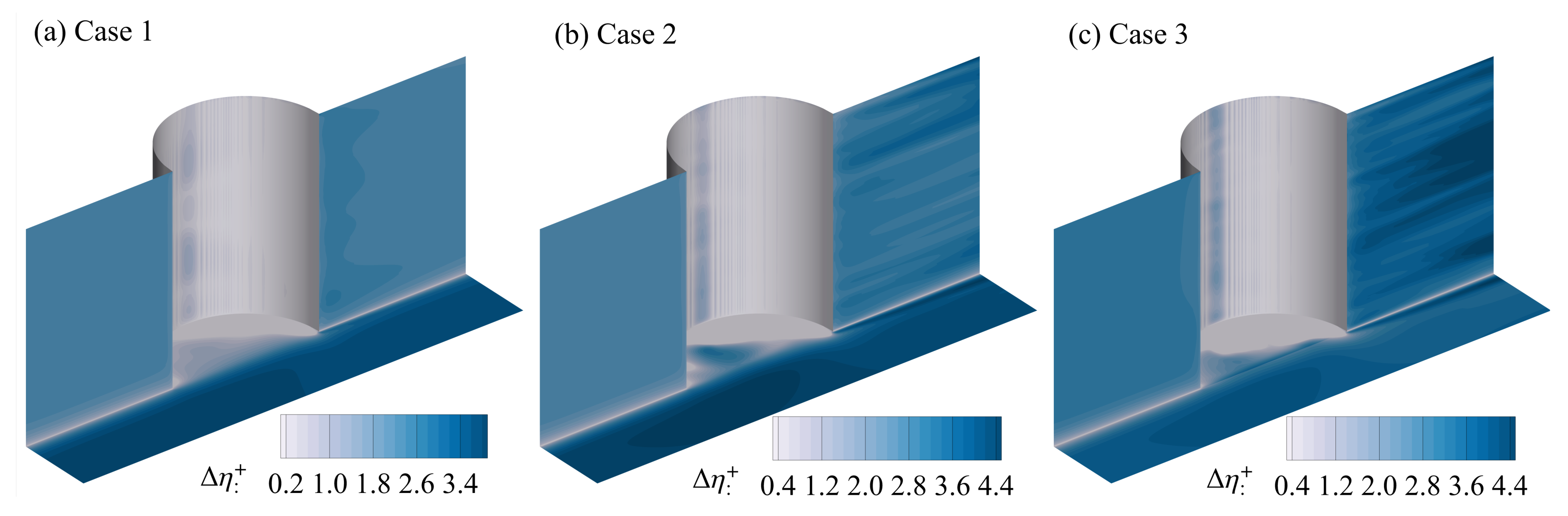
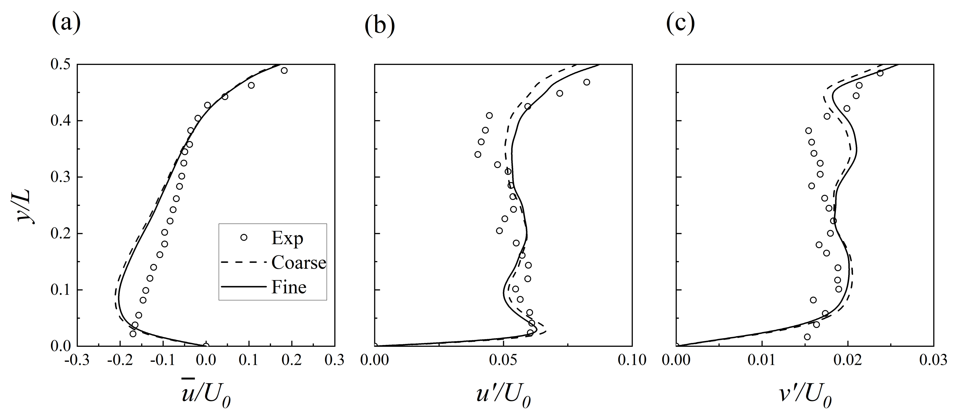
3.1. Verification

Time-averaged statistics from Case 1 are compared with experimental measurements in Figure 3, including profiles of u ¯ / U 0 , u / U 0 , and v / U 0 along the center radial (spanwise) line. The solid lines represent the results obtained using the fine grid defined in the previous Computational Setup Section, whereas the dashed lines correspond to those from a coarse grid with doubled grid spacings. The coarse grid slightly underpredicts the mean velocity compared to the fine grid. In terms of turbulence intensity, the coarse grid yields higher values near the bed but lower values within the shear layer. However, the impact of grid refinement on the simulation accuracy is not substantial, as the fine grid is already adequately resolved. Accordingly, all subsequent plots and analyses in this paper are based on the results of the fine-grid simulation.
Due to the recirculation inside the cavity, negative streamwise velocities are observed for y / L < 0.35 in both the experimental and LES results. However, LES slightly overpredicts the backflow strength near the cavity bottom. The maximum discrepancy occurs around y / L = 0.1 , with a relative error of up to 35%, whereas LES matches the PIV measurements well in the upper region of the cavity. This deviation is primarily attributed to inherent limitations of 2D-PIV in resolving near-wall flow, where strong velocity gradients and sparse seeding particles can bias measurements. In particular, the measured streamwise velocity increases almost linearly from the cavity bottom, while the LES profile exhibits a more physically consistent curvature near the wall. Both streamwise and spanwise turbulence intensities remain relatively constant within the recirculation zone but show a marked increase in the upper region of the cavity. In the transitional region ( 0.3 < y / L < 0.4 ), LES predictions of turbulence intensity exceed the experimental values by 20–30%, which may be partially attributed to the relatively low flow rate and spatial resolution of the experimental setup. Overall, the favorable agreement between LES and experimental data supports the capability of LES in accurately resolving the mean and turbulent flow features within a semi-circular cavity.

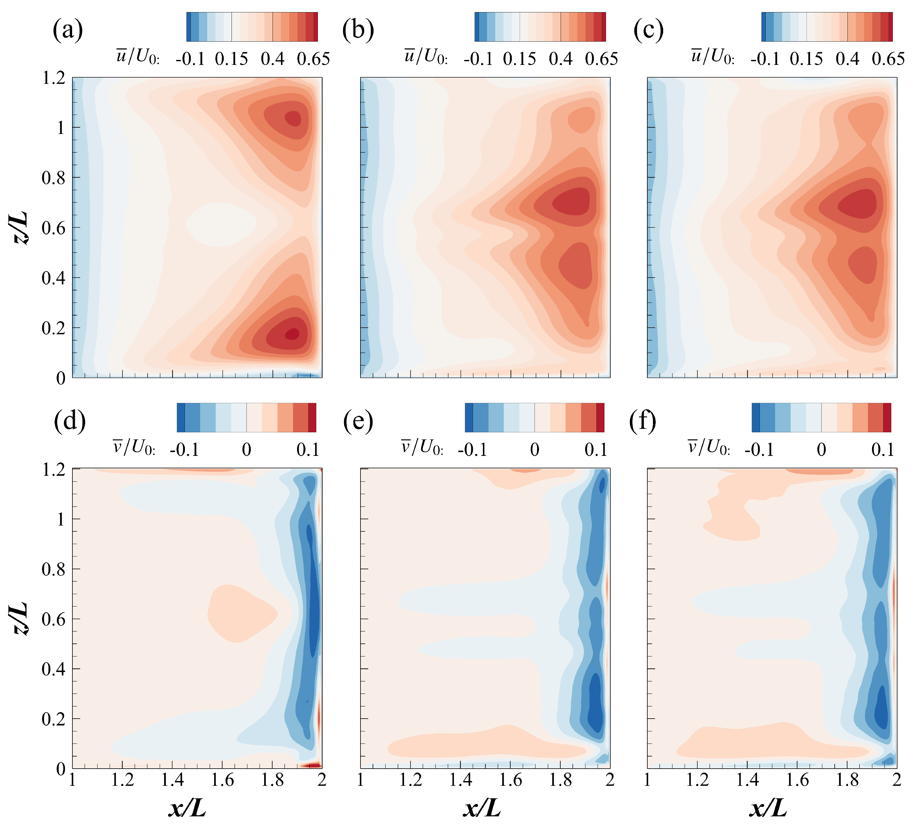
3.2. Time-Averaged Flow Structures

The time-averaged flow field in the semi-circular cavity and adjacent main channel region is illustrated in Figure 4 at the mid-depth horizontal plane ( z / h = 0.5). The left column presents the normalized streamwise velocity overlaid with streamlines, while the right column shows the normalized spanwise velocity. Streamlines in the main channel remain nearly parallel, except for localized distortions near the trailing edge of the cavity. The incoming boundary-layer flow separates at the leading edge of the cavity, develops into a shear layer along the channel–cavity interface, and impinges upon the trailing edge, where it is deflected into the cavity along the wetted perimeter. This deflection results in the formation of a prominent negative streamwise velocity region. After reaching the bottom point, the reversed flow turns upward and merges with the incoming shear layer, forming a closed-loop clockwise circulation, referred to as the MV, which occupies the majority of the cavity. The corner vortex (CV) forms near the leading edge of the semi-circular cavity and is the only secondary structure caused by the absence of orthogonal bottom corners unlike in rectangular cavities [27,61]. The overall flow pattern inside the cavity remains qualitatively similar across all three cases, aligning with characteristics of the skimming flow regime [62]. However, the velocity distributions and vortical structures exhibit significant variations with respect to the Reynolds number.
As the Reynolds number increases from 12,000 to 17,000, the most prominent change is the displacement of the MV core from the downstream cavity corner ( x / L = 1.85 ) to a location slightly upstream of the cavity’s bottom center ( x / L = 1.45 ), as seen by comparing Figure 4a,c. A similar vortex core migration was reported in previous studies investigating the effects of Reynolds number on rectangular cavity flows [19]. At higher R e values, inertial forces increasingly outweigh viscous effects and promote a stronger momentum transfer from the shear layer into the cavity. This leads to a steeper velocity gradient along the wetted perimeter, as shown in Figure 4c, and expands the region of negative spanwise velocity, as illustrated in Figure 4e. To maintain momentum and pressure balance, the MV core shifts toward the low-pressure zone near the cavity bottom. The CV at the upstream corner also grows significantly. Its spatial extent expands from a small core (diameter ≈ 0.01L) in Figure 4a to a broader zone spanning 0.4 < y / L < 0.5 in Figure 4c. Although Cases 1 and 2 show marked differences in their time-averaged flow fields, Cases 2 and 3 appear remarkably similar. In Case 3, the MV core moves only slightly upstream (about 0.1L), while the size of the CV remains nearly constant. The streamwise and spanwise velocities within the recirculating region show mild enhancements. The similarity between Cases 2 and 3 indicates that a dynamic equilibrium has formed near the MV core, where pressure gradients, velocity shear, and wall damping collectively prevent further displacement.
The time-averaged velocity distributions at the cavity–main channel interface for the three cases are shown in Figure 5. Under the lower Reynolds number in Case 1, the flow field exhibits near symmetry about the mid-height plane ( z / L = 0.6 ), as seen in Figure 5a. The highest streamwise velocity appears near the upstream and downstream corners, while peak spanwise velocity occurs along the mid-height line. Blue contours of spanwise velocity highlight fluid entrainment into the cavity, with a typical entrainment width of approximately one-tenth the cavity mouth width. However, this width increases significantly near the top and bottom boundaries, reaching up to four-fifths of the cavity width. In Cases 2 and 3, corresponding to higher Reynolds numbers, the velocity fields are nearly identical but deviate notably from Case 1. The region of maximum streamwise velocity shifts upward, peaking around z / L = 0.7 in Figure 5b,c, with a secondary maximum symmetrically located near z / L = 0.5 . The maximum spanwise velocity is concentrated along the downstream sidewall in the range 0.2 < y / L < 0.4 , as shown in Figure 5e,f. The vertical variations in streamwise and spanwise velocities confirm the three-dimensionality of the cavity flow [63,64]. The structure of the mean flow and vortex distribution changes considerably across vertical layers, and these Reynolds number-dependent vertical variations further contribute to the observed shift in the vortex’s core position.

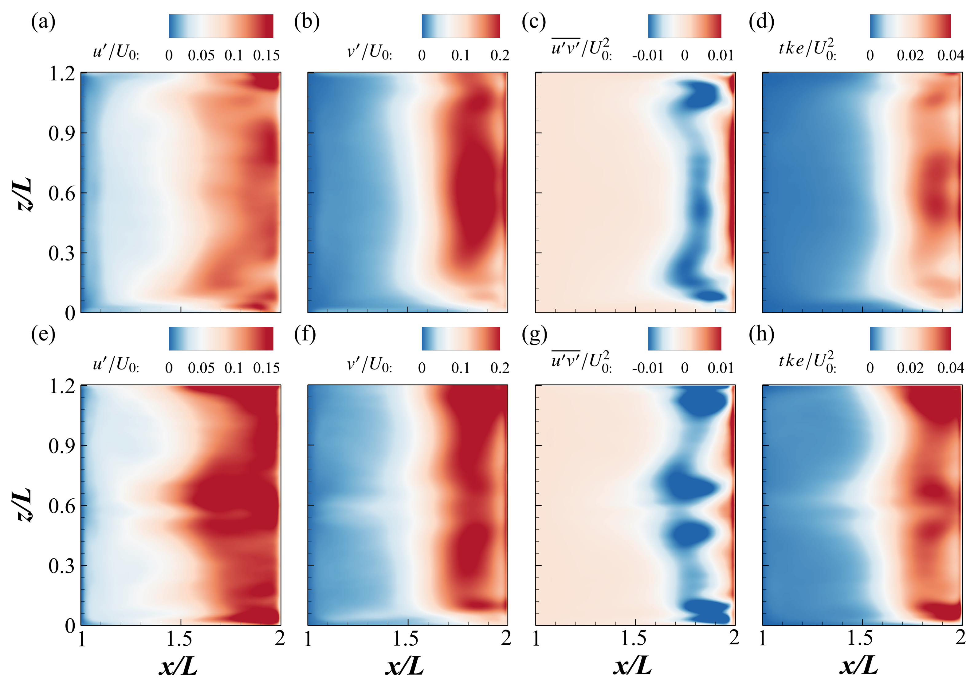
3.3. Second-Order Turbulence Statistics

Figure 6 compares the streamwise turbulence intensity ( u / U 0 ), spanwise turbulence intensity ( v / U 0 ), and Reynolds shear stress ( u v ¯ / U 0 2 ) between Case 1 and Case 2 at the mid-depth horizontal plane. Case 3 is omitted due to its close similarity to Case 2. The turbulence statistics reveal two primary sources of turbulence: (1) the shear layer at the interface between the main channel and the cavity, and (2) a jet-like inflow penetrating the cavity along the wetted perimeter [36]. As shown in Figure 6a–d, turbulence intensities are concentrated along the shear layer. Streamwise flow instabilities emerge in three distinct regions: (1) the central part of the cavity, where recirculating flow from the MV reattaches to the shear layer, inducing unsteady acceleration; (2) the trailing corner, where flow impingement causes local deceleration and instability; and (3) the outer turbulent boundary layer near the downstream wall. Figure 6b shows that the increasing Reynolds number amplifies the streamwise turbulence intensity within the shear layer. Additionally, the upstream shift of the MV core displaces the high-turbulence region further upstream. For example, the u / U 0 = 0.1 contour boundary moves from x / L = 1.35 in Figure 6a to x / L = 1.15 in Figure 6b.
Positive contours of Reynolds shear stress ( u v ¯ ) are distributed along the wetted perimeter of the downstream cavity, reflecting the contribution of turbulence to wall shear stress [38]. In contrast, negative contours are primarily concentrated within the downstream half of the cavity mouth, indicating momentum transfer from the outer high-momentum region to the inner low-momentum region via the shear layer. Notably, in Case 2, negative u v ¯ values appear along the upstream curved wall from x / L = 1.1 to 1.3 , as shown in Figure 6f. This region corresponds to the boundary layer separation of the recirculating backflow illustrated in Figure 4c. In contrast, this feature is absent in the low-Reynolds-number Case 1 (Figure 6e), where the recirculating streamlines remain attached to the wall up to the leading-edge CV. Although the CV contributes minimally to the streamwise and spanwise turbulence intensities, its presence is evident through localized positive u v ¯ contours near the cavity corner, highlighting its role in local Reynolds shear stress generation.
Figure 7 compares turbulence statistics across the transition plane between the main channel and the lateral cavity for Cases 1 and 2. The distributions of both turbulence intensity components and turbulent kinetic energy (TKE) are nearly two-dimensional, indicating lower turbulence levels in the upstream section of the cavity. However, downstream of x / L = 1.6 , turbulence activity increases rapidly. The influence of Reynolds number is more pronounced for streamwise turbulence intensity ( u / U 0 ) than for spanwise ( v / U 0 ), consistent with experimental measurements [35]. While the spatial extent of v / U 0 > 0.15 remains similar between the two cases, both the coverage and magnitude of u / U 0 > 0.1 in Figure 7e exceed those in Figure 7a, contributing to the higher TKE observed in Figure 7h, where t k e = u i u i / 2 . In Case 1, the Reynolds shear stress contours along the cavity mouth are predominantly negative and exhibit vertically uniform distributions. In Case 2, however, four distinct high-value regions ( u v ¯ / U 0 2 0.1 ) emerge near the upper, middle, and bottom layers ( z / L = 0.05 , 0.50, 0.70, and 0.95), indicating enhanced three-dimensionality of turbulence at higher Reynolds numbers. Additionally, localized positive Reynolds shear stress appears near the downstream edge at x / L = 2 in Figure 7e,g. This feature is attributed to cavity-corner-induced effects and is more clearly illustrated in Figure 6e,f.

3.4. Instantaneous Turbulent Flow Structures

Figure 8 presents instantaneous pressure (p) contours overlaid with velocity vectors of the horizontal components (u) and (v) at the mid-depth plane for Cases 1 and 2, with snapshots taken at 0.20 s intervals. In both cases, visible unsteady pressure bubbles emerge in the mid-section of the cavity mouth while upstream velocity vectors remain nearly parallel, indicating a steady shear layer. Spanwise perturbations from the MV backflow gradually destabilize the shear layer and trigger the onset of Kelvin–Helmholtz (KH) instability. Initial vortex structures are subtle but grow rapidly in size and energy through interactions with the surrounding flow, propagating downstream along the cavity mouth. The KH vortices play a dominant role in driving mass and momentum exchange between the main stream and the cavity: negative-pressure cores entrain high-momentum channel flow into the cavity, while positive-pressure regions eject cavity fluid to the channel. At t + 0.6 s, KH vortices reach x / L = 1.9 with a maximum diameter of approximately 0.14 L . As approaching the trailing corner, vortices shrink and core negative pressure descends. Upon impinging on the downstream wall, part of the vortex structure is entrained into the cavity as small-scale secondary vortices (SVs) while the remaining portion merges into the near-wall flow of the main channel. This process governs turbulent scalar transport resembling other types of skimming flow but exhibiting a slight difference from the early stage in flows past a series of cavities or groynes. In such configurations, KH vortices originate at the upstream corner because the near-wall inflow is fully perturbed after passing multiple upstream structures. In contrast, the incoming near-wall flow for the isolated cavity herein remains a steady boundary layer of sufficient thickness. As the boundary layer transitions into a shear layer, its initial stability is preserved across the upstream section of the cavity mouth, resulting in lower turbulence levels as previously shown in Figure 6.
The evolution of Kelvin–Helmholtz (KH) vortices follows a similar pattern in Cases 1 and 2. However, the vortex core pressure magnitude in Case 2 is elevated due to stronger inertial forces at equivalent stages. Secondary vortices (SVs) propagate from the impingement location into the cavity along the wetted perimeter. In Case 1, SVs appear only in two consecutive snapshots, initially forming at y / L = 0.4 and dissipating rapidly before reaching y / L = 0.3 . This rapid dissipation is attributed to insufficient energy transfer from KH vortices to SVs during impingement, limiting travel length to < 0.1 L . In contrast, Case 2 exhibits persistent SVs in all snapshots, propagating from y / L = 0.42 to y / L = 0.16 . The intensified jet-like flow in Case 2 drives SVs deeper into the cavity, thereby inducing migration of the MV core from the trailing corner vicinity in Figure 4a to the cavity center in Figure 4c.
To better visualize the vortex structures around and inside the cavity, Figure 9 displays iso-surfaces of the instantaneous Q-criterion colored by a streamwise velocity for Case 1. The KH vortices originate from the mid-section of the cavity mouth as a result of spanwise perturbations in the shear layer. Due to their inherently three-dimensional nature, KH vortices maintain a relatively coherent vertical structure across the water depth during downstream convection as observed in the side view. The top view reveals a distinct velocity contrast between low-velocity cavity flow and high-velocity main-channel flow through color contours on KH vortex rollers. At the trailing corner, KH vortices are divided into high-momentum attached vortices and low-momentum SVs. Attached vortices are advected downstream along the sidewall, partially evolving into hairpin vortices. The turbulence level near the downstream sidewall is significantly elevated due to the uniform distribution of coherent structures in contrast to the steady boundary layer on the upstream sidewall. If a series of consecutive cavities were present downstream, KH vortices could potentially be triggered at the leading edge of each cavity. SVs characterized by negative (blue) streamwise velocity and small-scale roller are mainly concentrated near the separation point. Few SVs propagate toward the cavity crest along the wetted perimeter. In addition, coherent structures near the leading corner are absent for CVs as their size is negligibly small in Case 1.
The power spectral density computed from the time series of the spanwise fluctuating velocity at four locations along the cavity mouth (at y / L = 0.5 ) at mid-depth is presented in Figure 10 for Case 1. The other two cases are not shown as they exhibit qualitatively similar trends. Transverse velocity spectra at all four locations reveal periodic shear layer oscillations at a dominant frequency f = 1.90 . In Case 1 and Case 3, the corresponding peak frequencies are f = 1.80 and f = 1.92 , respectively. However, the spectral energy at the peak frequency increases by 42 times from the second ( x / L = 1.4 ) to the fourth point ( x / L = 1.8 ). In the upstream half of the cavity mouth, turbulence in the shear layer remains underdeveloped and energy dissipation is primarily governed by viscosity. Insufficient scale separation prevents the formation of a Kolmogorov inertial subrange, bypassing intermediate scales to directly feed energy into dissipation. Conversely, the shear layer undergoes progressive energy cascade formation in the downstream half of the cavity mouth, eventually exhibiting a localized −5/3 spectral slope beyond the peak frequency. These observations are consistent with the experimental findings of Grace et al. [31], who reported a gradual transition to turbulence and increased Reynolds shear stress downstream in cases with a laminar incoming boundary layer. In addition to the primary energy peak associated with the large-scale coherent structures, secondary peaks are also present due to the interaction between the undulant shear layer and the fluctuating MV in the cavity.

4. Conclusions

This study employed high-resolution large-eddy simulation (LES) to investigate the flow dynamics and momentum exchange mechanisms within a lateral semi-circular cavity subjected to longshore current. The simulation results are validated against laboratory data, confirming the model’s capability to capture key turbulence statistics and cavity-induced recirculation. Key findings are as follows:
(1)
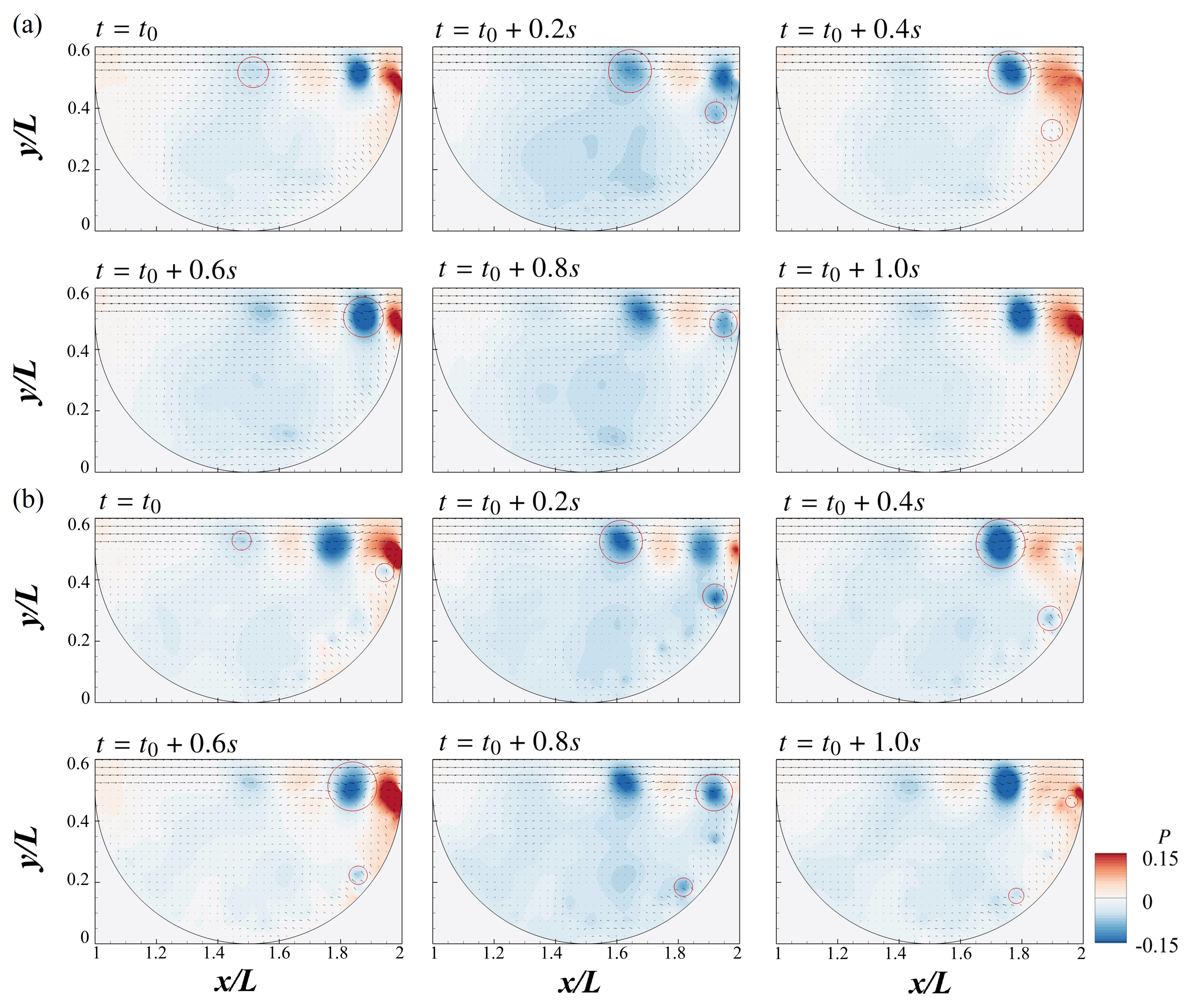
The time-averaged flow field features a dominant MV and a small upstream CV. With increasing Reynolds number, the MV core shifts upstream and shear layer interactions intensify, modifying the internal recirculation dynamics.
(2)
As R e increases from 12 , 000 to 17 , 000 , turbulence intensities and Reynolds shear stresses increase significantly near the cavity boundaries and shear interface, enhancing momentum exchange and mixing. However, a further increase to R e = 22 , 000 leads to a minimal change, indicating a transition toward a quasi-equilibrium regime.
(3)
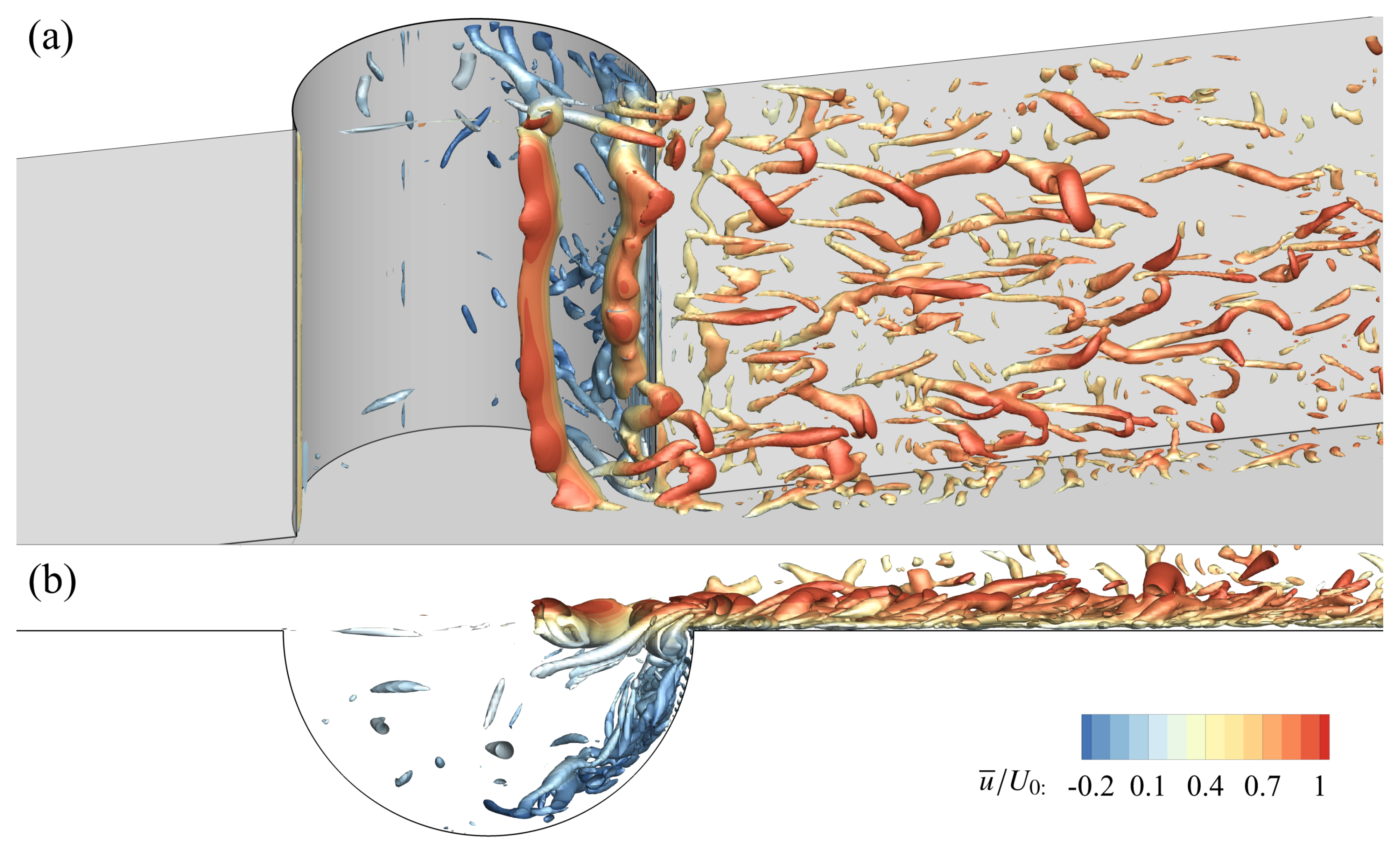
Instantaneous flow structures visualized by the Q-criterion reveal coherent KH vortices forming at the cavity mouth, with intensified secondary vortex (SV) generation and penetration at higher Reynolds numbers.
(4)
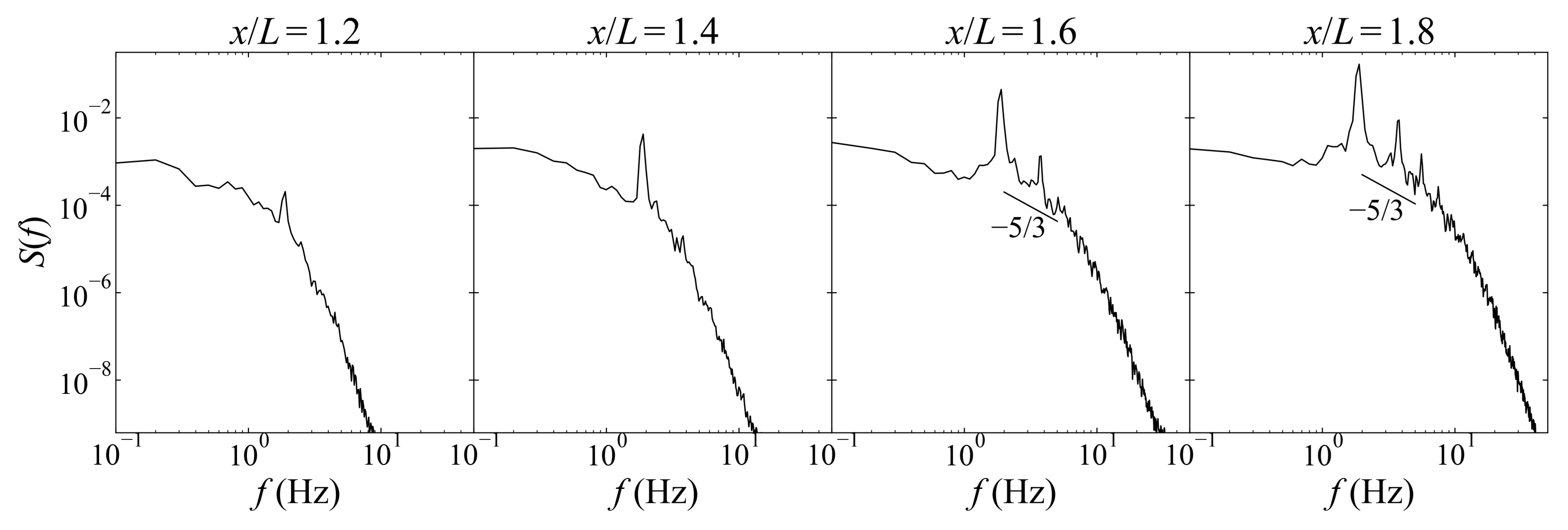
The spectral analysis of spanwise velocity fluctuations reveals dominant KH instability frequencies governing the periodic transport of momentum and vorticity into the cavity. Fully developed turbulence emerges downstream of the cavity mouth, where an inertial subrange with a localized −5/3 slope appears. In contrast, the upstream region remains viscosity-dominated with underdeveloped shear layer turbulence.
The semi-circular cavity investigated in this study serves as an idealized representation of natural coastal lateral cavities under longshore current. The use of IBM in the present simulations was intended as a preparatory step toward modeling more complex, irregularly shaped cavities found in real-world settings. Future work will focus on extending the current approach to cavities with realistic geometries and bathymetries.

Author Contributions

Conceptualization, Y.G., Y.X. and J.M.; methodology, Y.G., Y.X. and J.D.; formal analysis, Y.X., H.Z. and Q.X.; writing—original draft preparation, Y.G., J.D. and L.H.; writing—review and editing, L.H. and J.M.; visualization, Y.G., Y.X., H.Z. and Q.X.; supervision, J.D. and L.H.; project administration, J.M. and L.H. All authors have read and agreed to the published version of the manuscript.

Funding

This work was supported by the National Natural Science Foundation of China (52279013) and National Key Research and Development Program of China (2023YFC3209200).

Data Availability Statement

Data can be obtained from the first author upon request.

Acknowledgments

The authors gratefully acknowledge the support from the funding listed above. We also appreciate the anonymous reviewers who gave comments to revise the paper.

Conflicts of Interest

Author Yun Xu was employed by the company Zhejiang Institute of Communications Co., Ltd., and author Qianshun Xu was employed by the company Yellow River Engineering Consulting Co., Ltd. The remaining authors declare that the research was conducted in the absence of any commercial or financial relationships that could be construed as potential conflicts of interest.

References

  1. MacMahan, J.H.; Thornton, E.B.; Reniers, A.J. Deterministic Coastal Morphological and Sediment Transport Modeling: A Review and Discussion. Rev. Geophys. 2010, 48, RG3001. [Google Scholar] [CrossRef]
  2. Falqués, A.; Calvete, D.; Dodd, N.; de Swart, H.E. Understanding Coastal Morphodynamic Patterns from Depth-Averaged Sediment Concentration. Rev. Geophys. 2014, 52, 201–237. [Google Scholar] [CrossRef]
  3. Guo, X.; Fan, N.; Liu, Y.; Liu, X.; Wang, Z.; Xie, X.; Jia, Y. Deep seabed mining: Frontiers in engineering geology and environment. Int. J. Coal Sci. Technol. 2023, 10, 23. [Google Scholar] [CrossRef]
  4. Guo, X.; Fan, N.; Zheng, D.; Fu, C.; Wu, H.; Zhang, Y.; Song, X.; Nian, T. Predicting impact forces on pipelines from deep-sea fluidized slides: A comprehensive review of key factors. Int. J. Min. Sci. Technol. 2024, 34, 211–225. [Google Scholar] [CrossRef]
  5. Eriksson, B.K.; van der Heide, K.; van de Koppel, M.; Piersma, T.; van der Veer, H.W.; Olff, H. Ecosystem Engineering and Biodiversity in Coastal Sediments. Helgol. Mar. Res. 2009, 63, 23–32. [Google Scholar] [CrossRef]
  6. Hall, A.E.; Herbert, R.J.; Britton, J.R.; Hull, S.L. Ecological Enhancement Techniques to Improve Habitat Heterogeneity on Coastal Defence Structures. Estuar. Coast. Shelf Sci. 2018, 210, 68–78. [Google Scholar] [CrossRef]
  7. Boyd, L.B.; Janus, L.L.; Casselman, J.M. Submerged Aquatic Vegetation in Cook’s Bay, Lake Simcoe. J. Gt. Lakes Res. 2011, 37, 93–100. [Google Scholar] [CrossRef]
  8. Castellanos-Galindo, G.A.; Wolff, M.; Saint-Paul, U. Multilevel Decomposition of Spatial and Environmental Effects on Nearshore Fish Assemblages in Tropical Semi-Enclosed Ecosystems. Estuar. Coast. Shelf Sci. 2020, 237, 106691. [Google Scholar] [CrossRef]
  9. Bird, E.C.F. Coastal Geomorphology: An Introduction, 2nd ed.; John Wiley & Sons: Hoboken, NJ, USA, 2008. [Google Scholar]
  10. Symonds, J.P.; Jones, R.M. The Influence of Geomorphology and Sedimentary Processes on Benthic Habitat Distribution and Littoral Sediment Dynamics, Geraldton, Western Australia. Estuar. Coast. Shelf Sci. 2009, 84, 527–537. [Google Scholar] [CrossRef]
  11. Eliot, M.; Eliot, G. Shoreline Salients, Cuspate Forelands and Tombolos on the Coast of Western Australia. J. Coast. Res. 2010, 26, 812–822. [Google Scholar]
  12. Bo, T.; Ralston, D.K. Frontogenesis, Mixing, and Stratification in Estuarine Channels with Curvature. J. Phys. Oceanogr. 2022, 52, 1333–1352. [Google Scholar] [CrossRef]
  13. Pasquaud, P.; Schinegger, J.; Blanchet, S. Estuarine Lateral Ecotones Shape Taxonomic and Functional Structure of Fish Assemblages. Estuar. Coast. Shelf Sci. 2024, 313, 109066. [Google Scholar] [CrossRef]
  14. Chapman, M.G.; Underwood, A.J. Scales of variation of gastropod densities over multiple spatial scales: Comparison of common and rare species. J. Exp. Mar. Biol. Ecol. 2007, 348, 91–102. [Google Scholar] [CrossRef]
  15. Browne, M.A.; Thompson, R.J.A.; Chapman, L.A. Designing for sedimentation: The role of urban structures in the accumulation and distribution of estuarine sediment. Mar. Ecol. Prog. Ser. 2014, 507, 15–30. [Google Scholar] [CrossRef]
  16. Uijttewaal, W.S.J.; Lehmann, D.; van Mazijk, A. Exchange processes between a river and its groyne fields: Model experiments. J. Hydraul. Eng. 2001, 127, 928–936. [Google Scholar] [CrossRef]
  17. Lesack, L.F.W.; Marsh, P. River-to-lake connectivities, water renewal, and aquatic habitat diversity in the Mackenzie River Delta. Water Resour. Res. 2010, 46, W12504. [Google Scholar] [CrossRef]
  18. Mignot, E.; Barthelemy, E.; Hurther, A. Coherent turbulent structures at the mixing-interface of a square open-channel lateral cavity. Phys. Fluids 2016, 28, 045102. [Google Scholar] [CrossRef]
  19. Chiang, T.P.; Sheu, W.H.; Hwang, R.R. Effect of Reynolds number on the eddy structure in a lid-driven cavity. Int. J. Numer. Methods Fluids 1998, 26, 557–579. [Google Scholar] [CrossRef]
  20. Chang, K.S.; Constantinescu, S.G.; Park, S. Analysis of the flow and mass transfer processes for the incompressible flow past an open cavity with a laminar and a fully turbulent incoming boundary layer. J. Fluid Mech. 2006, 561, 113–145. [Google Scholar] [CrossRef]
  21. Faure, T.M.; Adrianos, P.; Lusseyran, F.; Pastur, L. Visualizations of the flow inside an open cavity at medium range Reynolds numbers. Exp. Fluids 2007, 42, 169–184. [Google Scholar] [CrossRef]
  22. Drost, K.; Jackson, T.; Haggerty, R.; Apte, S.V. RANS Predictions of Turbulent Scalar Transport in Dead Zones of Natural Streams. In Proceedings of the ASME 2012 Fluids Engineering Division Summer Meeting, Rio Grande, PR, USA, 8–12 July 2012; pp. 1167–1177. [Google Scholar] [CrossRef]
  23. Drost, K.J.; Apte, S.V.; Haggerty, R.; Jackson, T.R. Parameterization of Mean Residence Times in Idealized Rectangular Dead Zones Representative of Natural Streams. J. Hydraul. Eng. 2014, 140, 04014035. [Google Scholar] [CrossRef]
  24. Brevis, W.; García-Villalba, M.; Niño, Y.N. Experimental and large eddy simulation study of the flow developed by a sequence of lateral obstacles. Environ. Fluid Mech. 2014, 14, 873–893. [Google Scholar] [CrossRef]
  25. Jackson, T.R.; Haggerty, R.; Apte, S.V.; Coleman, A.; Drost, K.J. Defining and measuring the mean residence time of lateral surface transient storage zones in small streams. Water Resour. Res. 2012, 48, W10501. [Google Scholar] [CrossRef]
  26. Jackson, T.R.; Haggerty, R.; Apte, S.V.; O’Connor, B.L. A mean residence time relationship for lateral cavities in gravel-bed rivers and streams: Incorporating streambed roughness and cavity shape. Water Resour. Res. 2013, 49, 3642–3650. [Google Scholar] [CrossRef]
  27. Constantinescu, G.; Sukhodolov, A.; McCoy, A. Mass exchange in a shallow channel flow with a series of groynes: LES study and comparison with laboratory and field experiments. Environ. Fluid Mech. 2009, 9, 587–615. [Google Scholar] [CrossRef]
  28. Juez, C.; Bühlmann, I.; Maechler, G.; Schleiss, A.J.; Franca, M.J. Transport of suspended sediments under the influence of bank macro-roughness. Earth Surf. Process. Landf. 2018, 43, 271–284. [Google Scholar] [CrossRef]
  29. McCoy, A.; Constantinescu, G.; Weber, L. A numerical investigation of coherent structures and mass exchange processes in channel flow with two lateral submerged groynes. Water Resour. Res. 2007, 43, W05445. [Google Scholar] [CrossRef]
  30. Weitbrecht, V.; Socofolosky, S.A.; Jirka, G.H. Experiments on mass exchange between groin fields and main stream in rivers. J. Hydraul. Eng. 2008, 134, 173–183. [Google Scholar] [CrossRef]
  31. Grace, S.M.; Dewar, W.G.; Wroblewski, D.E. Experimental investigation of the flow characteristics within a shallow wall cavity for both laminar and turbulent upstream boundary layers. Exp. Fluids 2004, 36, 791–804. [Google Scholar] [CrossRef]
  32. Crook, S.D.; Lau, T.C.W.; Kelso, R.M. Three-dimensional flow within shallow, narrow cavities. J. Fluid Mech. 2013, 735, 587–612. [Google Scholar] [CrossRef]
  33. Engelen, L.; Perrot-Minot, C.; Mignot, E.; Rivière, N.; De Mulder, T. Lagrangian study of the particle transport past a lateral, open-channel cavity. Phys. Fluids 2021, 33, 013303. [Google Scholar] [CrossRef]
  34. Engelhardt, C.; Krüger, A.; Wüst, A.; Mohrholz, A. A study of phytoplankton spatial distributions, flow structure and characteristics of mixing in a river reach with groynes. J. Plankton Res. 2004, 26, 1351–1366. [Google Scholar] [CrossRef]
  35. Ozalp, C.; Pinarbasi, A.; Sahin, B. Experimental measurement of flow past cavities of different shapes. Exp. Therm. Fluid Sci. 2010, 34, 505–515. [Google Scholar] [CrossRef]
  36. Jackson, T.R.; Apte, S.V.; Haggerty, R.; Budwig, R. Flow Structure and Mean Residence Times of Lateral Cavities in Open Channel Flows: Influence of Bed Roughness and Shape. Environ. Fluid Mech. 2015, 15, 1069–1100. [Google Scholar] [CrossRef]
  37. Koseff, J.R.; Street, R.L. The Lid-Driven Cavity Flow: A Synthesis of Qualitative and Quantitative Observations. J. Fluids Eng. 1984, 106, 390–398. [Google Scholar] [CrossRef]
  38. Ouro, P.; Juez, C.; Franca, M. Drivers for mass and momentum exchange between the main channel and river bank lateral cavities. Adv. Water Resour. 2020, 137, 103511. [Google Scholar] [CrossRef]
  39. Liu, H.; Liu, M.; Ai, Y.; Huai, W. Turbulence Characteristics in Partially Vegetated Open Channels with Alternating Sparse and Dense Patches. Phys. Fluids 2024, 36, 015130. [Google Scholar] [CrossRef]
  40. Chang, K.; Constantinescu, G.; Park, S.O. Comparison of Large Eddy Simulation, Detached Eddy Simulation and Unsteady RANS Numerical Predictions of Flow Past a Bottom River Cavity. In Proceedings of the 32nd IAHR World Congress, Venice, Italy, 1–6 July 2007. [Google Scholar]
  41. Ouro, P.; Cea, L.; Croquer, S.; Dong, W.; Garcia-Feal, O.; Navas-Montilla, A.; Rogers, B.D.; Uchida, T.; Juez, C. Benchmark of Computational Hydraulics Models for Open-Channel Flow with Lateral Cavities. J. Hydraul. Res. 2024, 62, 441–460. [Google Scholar] [CrossRef]
  42. Liu, M.; Yuan, S.; Tang, H.; Huai, W.; Yan, J. Investigation of turbulence and interfacial exchange features of the gap area within the fully developed Shallow-Submerged canopy flow. J. Hydrol. 2024, 643, 131938. [Google Scholar] [CrossRef]
  43. Liu, M.; Huai, W.; Tang, H.; Wang, Y.; Yuan, S. Numerical study of mean and turbulent flow adjustments in open channels with limited near-bank vegetation patches. Phys. Fluids 2024, 36, 095117. [Google Scholar] [CrossRef]
  44. Uhlmann, M. An immersed boundary method with direct forcing for the simulation of particulate flows. J. Comput. Phys. 2005, 209, 448–476. [Google Scholar] [CrossRef]
  45. Gong, Y.; Stoesser, T.; Mao, J.; McSherry, R. LES of flow through and around a finite patch of thin plates. Water Resour. Res. 2019, 55, 7587–7605. [Google Scholar] [CrossRef]
  46. Luo, Q.; Dolcetti, G.; Stoesser, T.; Tait, S. Water surface response to turbulent flow over a backward-facing step. J. Fluid Mech. 2023, 966, A18. [Google Scholar] [CrossRef]
  47. Guo, X.; Liu, X.; Zheng, T.; Zhang, H.; Lu, Y.; Li, T. A mass transfer-based LES modelling methodology for analyzing the movement of submarine sediment flows with extensive shear behavior. Coast. Eng. 2024, 191, 104531. [Google Scholar] [CrossRef]
  48. Liu, Y.; Tang, Z.; Huang, L.; Stoesser, T.; Fang, H. On the role of the Froude number on flow, turbulence, and hyporheic exchange in open-channel flow through boulder arrays. Phys. Fluids 2024, 36, 095141. [Google Scholar] [CrossRef]
  49. Dai, J.; Mao, J.q.; Gong, Y.q.; Gao, H. Effect of triangular baffle designs on flow dynamics and sediment transport within standard box culverts. J. Hydrodyn. 2024, 36, 1142–1154. [Google Scholar] [CrossRef]
  50. Dai, J.; Xu, Q.; Gong, Y.; Lu, Y.; Liu, X.; Mao, J. An LES Investigation of Flow Field Around the Cuboid Artificial Reef at Different Angles of Attack. J. Mar. Sci. Eng. 2025, 13, 463. [Google Scholar] [CrossRef]
  51. Fadlun, E.; Verzicco, R.; Orlandi, P.; Mohd-Yusof, J. Combined immersed-boundary finite-difference methods for three-dimensional complex flow simulations. J. Comput. Phys. 2000, 161, 35–60. [Google Scholar] [CrossRef]
  52. Nicoud, F.; Ducros, F. Subgrid-scale stress modelling based on the square of the velocity gradient tensor. Flow Turbul. Combust. 1999, 62, 183–200. [Google Scholar] [CrossRef]
  53. Peskin, C. Fluid dynamics of heart valves: Experimental, theoretical, and computational methods. Annu. Rev. Fluid Mech. 1982, 14, 235–259. [Google Scholar] [CrossRef]
  54. Christou, A.; Stoesser, T.; Xie, Z. A large-eddy-simulation-based numerical wave tank for three-dimensional wave-structure interaction. Comput. Fluids 2021, 231, 105179. [Google Scholar] [CrossRef]
  55. Chorin, A.J. Numerical solution of the Navier-Stokes equations. Math. Comput. 1968, 22, 745–762. [Google Scholar] [CrossRef]
  56. Cevheri, M.; McSherry, R.; Stoesser, T. A local mesh refinement approach for large-eddy simulations of turbulent flows. Int. J. Numer. Methods Fluids 2016, 82, 261–285. [Google Scholar] [CrossRef]
  57. Ouro, P.; Fraga, B.; Lopez-Novoa, U.; Stoesser, T. Scalability of an Eulerian–Lagrangian large-eddy simulation solver with hybrid MPI/OpenMP parallelisation. Comput. Fluids 2019, 179, 123–136. [Google Scholar] [CrossRef]
  58. Zhang, Y.; Wang, L.; Li, X.; Chen, H. Effects of vegetation density on flow, mass exchange and sediment transport in lateral cavities. J. Hydrol. 2024, 631, 129567. [Google Scholar]
  59. Jarrin, N.; Benhamadouche, S.; Laurence, D.; Prosser, R. A synthetic-eddy-method for generating inflow conditions for large-eddy simulations. Int. J. Heat Fluid Flow 2006, 27, 585–593. [Google Scholar] [CrossRef]
  60. Adzic, F.; Stoesser, T.; Liu, Y.; Xie, Z. Large-eddy simulation of supercritical free-surface flow in an open-channel contraction. J. Hydraul. Res. 2022, 60, 628–644. [Google Scholar] [CrossRef]
  61. Fang, H.; Bai, J.; He, G.; Zhao, H. Calculations of Nonsubmerged Groin Flow in a Shallow Open Channel by Large-Eddy Simulation. J. Eng. Mech. 2014, 140, 04014016. [Google Scholar] [CrossRef]
  62. Meile, T.; Boillat, J.L.; Schleiss, A.J. Flow Resistance Caused by Large-Scale Bank Roughness in a Channel. J. Hydraul. Eng. 2011, 137, 1588–1597. [Google Scholar] [CrossRef]
  63. Samantaray, S.S.; Das, D. High Reynolds number incompressible turbulent flow inside a lid-driven cavity with multiple aspect ratios. Phys. Fluids 2018, 30, 075103. [Google Scholar] [CrossRef]
  64. Dong, W.; Uchida, T. Role of three-dimensional vortex motions on horizontal eddies in an open-channel cavity. Environ. Fluid Mech. 2024, 24, 539–566. [Google Scholar] [CrossRef]
Figure 1. Geometric configuration of the computational domain, which corresponds to the semi-circular cavity in the laboratory work of Ozalp et al. [35].
Jmse 13 00859 g001
Figure 2. Contours of the dimensionless wall distance around the cavity section at different Reynolds numbers.
Jmse 13 00859 g002
Figure 3. Transverse profiles of time-average streamwise velocity u ¯ / U 0 (a) and streamwise (b) and spanwise turbulence intensities (c) at x / L =1.5. Comparison between experiments and the present Case 1 LES results. Experimental data (circles), coarse-mesh LES (dashed line), and fine-mesh LES (solid line).
Jmse 13 00859 g003
Figure 4. Distribution of normalized time-averaged streamwise ( u ¯ / U 0 ) and spanwise velocities v ¯ / U 0 at the mid−depth plane for the three cases. Streamlines are only plotted on the contours of streamwise velocity for simplicity. (a,b) for Case 1; (c,d) for Case 2; (e,f) for Case 3.
Jmse 13 00859 g004
Figure 5. Distribution of normalized time-averaged streamwise u ¯ / U 0 (the upper row) and spanwise velocities v ¯ / U 0 (the lower row) through the mouth of the cavity at y / L = 0.5 for the three cases. (a,d) for Case 1; (b,e) for Case 2; (c,f) for Case 3.
Jmse 13 00859 g005
Figure 6. Distribution of normalized streamwise u / U 0 and spanwise v / U 0 turbulence intensities and Reynolds shear stress u v ¯ / U 0 2 at the mid-depth plane. The left column is for Case 1 and the right one is for Case 2. (a,c,e) for Case 1; (b,d,f) for Case 2.
Jmse 13 00859 g006
Figure 7. Distribution at a plane through the mouth of the cavity at y/L = 0.5 for Case 1 (upper row) and Case 2 (lower row); (a,e) are the streamwise turbulence intensity u / U 0 ; (b,f) are the spanwise turbulence intensity u / U 0 ; (c,g) are Reynolds shear stress u v ¯ / U 0 2 ; (d,h) are total kinetic energy t k e / U 0 2 .
Jmse 13 00859 g007
Figure 8. Contours of instantaneous pressure, p, with velocity vectors of instantaneous streamwise (u) and spanwise (v) components for Case 1 (a) and Case 2 (b). The snapshots have a time lapse of 0.20 s among them and the the red circles indicate the outlines of counter-clockwise vortices.
Jmse 13 00859 g008
Figure 9. Instantaneous flow structures represented by iso-surfaces of the Q criterion with normalized streamwise velocity (a) in the side view and (b) in the top view for Case 1.
Jmse 13 00859 g009
Figure 10. Power spectral density of the spanwise fluctuating velocity time-series at four spatial samples located at different transverse locations along the cavity mouth ( y / L = 0.5 ) at half depth for Case 2.
Jmse 13 00859 g010
Table 1. Details of grid resolution and the hydrodynamic conditions for the cases studied.
Case Δ x = Δ y (mm) Δ z (mm) U 0 (m/s) Re Fr
10.6251.00.1212,0000.11
20.6251.00.1717,0000.15
30.6250.50.2222,0000.20
Disclaimer/Publisher’s Note: The statements, opinions and data contained in all publications are solely those of the individual author(s) and contributor(s) and not of MDPI and/or the editor(s). MDPI and/or the editor(s) disclaim responsibility for any injury to people or property resulting from any ideas, methods, instructions or products referred to in the content.

