The Local Path Planning Algorithm for Amphibious Robots Based on an Improved Dynamic Window Approach

Abstract

The autonomous navigation capability of amphibious robots in complex water–land environments is a key technology. However, with the existing local path planning methods, it is difficult to meet the autonomous navigation needs of amphibious robots. To address the shortcomings of unreachable targets, poor adaptability, and limited planning range in a water–land environment, this study proposes a local path planning method based on the improved dynamic window approach (IDWA). A water–land hybrid kinematic model and an obstacle expansion method are applied in the new approach. The improved dynamic window approach enhances the automatic adaptability of complex water–land environments. The improved evaluation function and distance cost function avoid overshooting at the target endpoint. The speed resolution adaptive adjustment algorithm improves the ability to pass through a complex multiple-obstacle area, and the dynamic obstacle prediction algorithm optimizes obstacle avoidance paths. The simulation and lake experiments demonstrate that compared to traditional DWA, the IDWA reduces task completion time by 32.99%, algorithm runtime by 35.29%, and path length by 10.78%. The heading angle variations are decreased by 9.92% while maintaining an average speed of 0.70 m/s in complex environments. The experimental results validate that the proposed approach can effectively plan safe and smooth paths in complex water–land environments with multiple moving obstacles.

1. Introduction

1.1. Background

Amphibious robots, owing to their ability to traverse across different domains, have emerged as a central theme in the research and development of marine exploration equipment [1,2]. Due to their expanding working space and capabilities, amphibious robots can be applied in underwater terrain exploration, resource prospecting, aquatic environment monitoring, disaster search and rescue, and scientific research.

Local path planning, one of the key technologies, is particularly important. Effective path planning ensures that amphibious unmanned vehicles can efficiently and safely reach the target and maximize their performance advantages, improving the efficiency and success rate of task execution. Traditional planning algorithms, however, are primarily designed for uniform environments and fail to address the complex challenges of water–land transitional operations. This research presents a novel navigation algorithm specifically engineered for autonomous amphibious platforms.

1.2. Problem Description

Unlike traditional robots that work in a single environment, amphibious robots can work both underwater and on land. Local path planning algorithms include traditional methods such as the artificial potential field (APF) method [3,4], rapidly exploring random trees (RRT) [5], and intelligent bionic algorithms like neural networks [6]. The APF method is prone to failure in path planning due to complex obstacles [7]. RRT is inefficient, which results in winding paths [8]. Neural networks are slow in complex environments and need much time to process data [9]. Consequently, these algorithms are unsuitable for the complex amphibious environments.

The dynamic window approach (DWA) is a real-time local obstacle avoidance algorithm that achieves dynamic obstacle avoidance by searching for the optimal velocity within the robot’s velocity space [10,11,12]. DWA offers two key benefits: fast computations and safe path generation. DWA has received extensive research attention. However, the algorithm has three major limitations: it is unable to reach targets, is poorly adapted to changing environments, and has a limited planning range [13,14,15,16].

Ming Yao et al. proposed an enhanced dynamic window method based on fuzzy logic. This model extends the evaluation capabilities of the dynamic window method, enhancing the smoothness of the generated path [17,18]. Guo et al. proposed an integrated approach combining an extended Kalman filter, nonlinear model predictive control, and a novel obstacle avoidance method, which enhances the robot navigation ability in uncertain dynamic environments [19]. Xiang’s team developed a fuzzy controller for dynamic weight control. Their method produces smoother and more stable paths. The improved system performs well in complex environments [20]. Matej Dobrevski et al. integrated DWA with deep learning by proposing a neural network to predict its weights. This method adjusts the appropriate robot motion weights by observing the current state of the environment, enabling the DWA to adapt to environmental changes [21]. Zhang Xin et al. enhanced intelligent dynamic path adjustment method for robots by implementing variable safety distances for different obstacles [15]. Hang Peng et al. enhanced the dynamic obstacle avoidance capability of robots by adding a minimum turning radius constraint to the velocity selection mechanism and incorporating a curvature maintenance evaluation metric into the assessment function, building upon the DWA [22].

In summary, the traditional DWA algorithm is only applicable to two-dimensional environments and cannot be applied to complex environments with multiple degrees of freedom on land and in water. There are disadvantages of DWA such as high sensitivity to evaluation parameters, poor dynamic obstacle avoidance ability, and unreachable targets.

This proposed IDWA in this study differs from that of previous studies in several key aspects:

• Environmental Adaptation: Unlike traditional DWA improvements that focus on either land or water environments, IDWA incorporates a water–land hybrid kinematic model that enables seamless transition between different mediums. This is particularly crucial for amphibious robots operating in complex water–land environments.
• Dynamic Resolution Control: Previous studies typically use fixed velocity resolution, which can be inefficient in varying obstacle densities. IDWA introduces an adaptive velocity resolution mechanism that automatically adjusts based on environmental complexity, improving both computational efficiency and path quality.
• Obstacle Prediction Integration: While some studies have addressed moving obstacles, IDWA uniquely combines kinematic modeling with dynamic obstacle prediction, making it particularly effective for complex water–land environments where obstacles may exhibit different movement patterns in different mediums.
• Multi-objective Optimization: Unlike previous approaches that use fixed evaluation parameters, IDWA employs adaptive weighting coefficients and introduces a distance cost function, specifically addressing the challenges of target reachability and endpoint overshooting in amphibious operations.

These innovations directly address the three major limitations of traditional DWA: unreachable targets, poor environmental adaptability, and limited planning range. The effectiveness of these improvements is demonstrated through comprehensive simulations and real-world experiments.

2. Model Construction

2.1. Hybrid Water–Land Kinematic Model

Traditional kinematic models are typically designed for single-environment robots, such as underwater vehicles using 6-DOF models or ground vehicles using 2D/3D models. However, these models are insufficient for amphibious robots that need to operate seamlessly in both aquatic and terrestrial environments. The key differences between our proposed hybrid model and existing approaches are as follows:

• Integration of multi-modal locomotion: Unlike single-environment models, our hybrid framework combines underwater (5-DOF) and land (3-DOF) motion characteristics into a unified model, enabling smooth transitions between different locomotion modes.
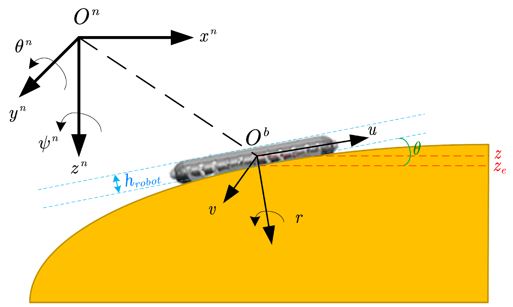
• Terrain-adaptive parameters: The model introduces terrain-specific parameters ($z_e$ and ${\theta }_e$) that dynamically adjust to varying slopes and elevations, allowing the robot to adapt to complex topographical changes in both water and land environments.
• Mode-specific constraints: The model incorporates different kinematic constraints for each locomotion mode, such as reduced degrees of freedom during water–land transitions and varying velocity and acceleration limits for different environments.
• Environmental adaptation: Through the hybrid structure, the model can automatically switch between appropriate kinematic parameters based on the current environment, ensuring optimal performance in both aquatic and terrestrial operations.

The motion of amphibious robots [23,24,25] in underwater, cross-domain, and land environments is described using two coordinate frames: the geodetic coordinate frame and the body coordinate frame as illustrated in Figure 1.

The kinematic model is used to relate the position and attitude parameters in the geodetic coordinate frame with the velocity parameters in the body coordinate frame [26,27]. The traditional six-degrees-of-freedom (DOF) kinematic model is shown in Equation (1) [28,29,30]:

$$\dot{\eta }=J_{\Theta }\left(\eta \right)\gamma$$

(1)

In the above equation, $\eta ={\left[P^n{\Theta }_{nb}\right]}^T$ represents the robot’s position and angle in the geodetic coordinate frame, $P^n={\left[xyz\right]}^T$ represents the robot’s three-dimensional position in the geodetic coordinate frame, and ${\Theta }_{nb}={\left[\varphi \theta \psi \right]}^T$ represents the Euler angles of the body coordinate frame relative to the geodetic frame. $\gamma ={\left[{\nu }^b{\omega }^b\right]}^T$ represents the robot’s velocity in the body coordinate frame, where ${\nu }^b={\left[uvw\right]}^T$ denotes the robot’s linear velocity in the body coordinate frame, and ${\omega }^b={\left[pqr\right]}^T$ denotes the robot’s angular velocity in the body coordinate frame. $J_{\Theta }\left(\eta \right)$ represents the transformation matrix from the body coordinate frame to the geodetic coordinate frame, including the position and angular rotation matrices, as shown in Equation (2):

$$\left[\begin{array}{c}\dot{P^n}\\ {\Theta }_{nb}\end{array}\right]=\left[\begin{array}{cc}{R}_b^n\left({\Theta }_{nb}\right)& 0_{33}\\ 0_{33}& T_{\Theta }\left({\Theta }_{nb}\right)\end{array}\right]\left[\begin{array}{c}{\nu }^b\\ {\omega }^b\end{array}\right]$$

(2)

In the above equation, the position rotation matrix $R_b^n\left({\Theta }_{nb}\right)$ and the attitude rotation matrix $T_{\Theta }\left({\Theta }_{nb}\right)$ are shown as in Equation (3):

$$\left\{\begin{array}{c}{R}_b^n\left({\Theta }_{nb}\right)=\left[\begin{array}{cc}A& B\end{array}\right]\hfill \\ T_{\Theta }\left({\Theta }_{nb}\right)=\left[\begin{array}{ccc}1& sin\varphi tan\theta & cos\varphi tan\theta \\ 0& cos\varphi & -sin\varphi \\ 0& sin\varphi /cos\theta & cos\varphi /cos\theta \end{array}\right]\hfill \\ A=\left[\begin{array}{cc}cos\theta cos\psi & -cos\theta sin\psi +sin\varphi sin\theta cos\psi \\ cos\theta sin\psi & cos\varphi cos\psi +sin\varphi sin\theta sin\psi \\ -sin\theta & sin\varphi cos\theta \end{array}\right]\hfill \\ B=\left[\begin{array}{c}sin\varphi sin\psi +cos\varphi sin\theta cos\psi \\ -sin\varphi cos\psi +cos\varphi sin\theta sin\psi \\ cos\varphi cos\theta \end{array}\right]\hfill \end{array}\right.$$

(3)

Based on the 6-DOF kinematic model, we establish the water and land kinematic models for the amphibious robot.

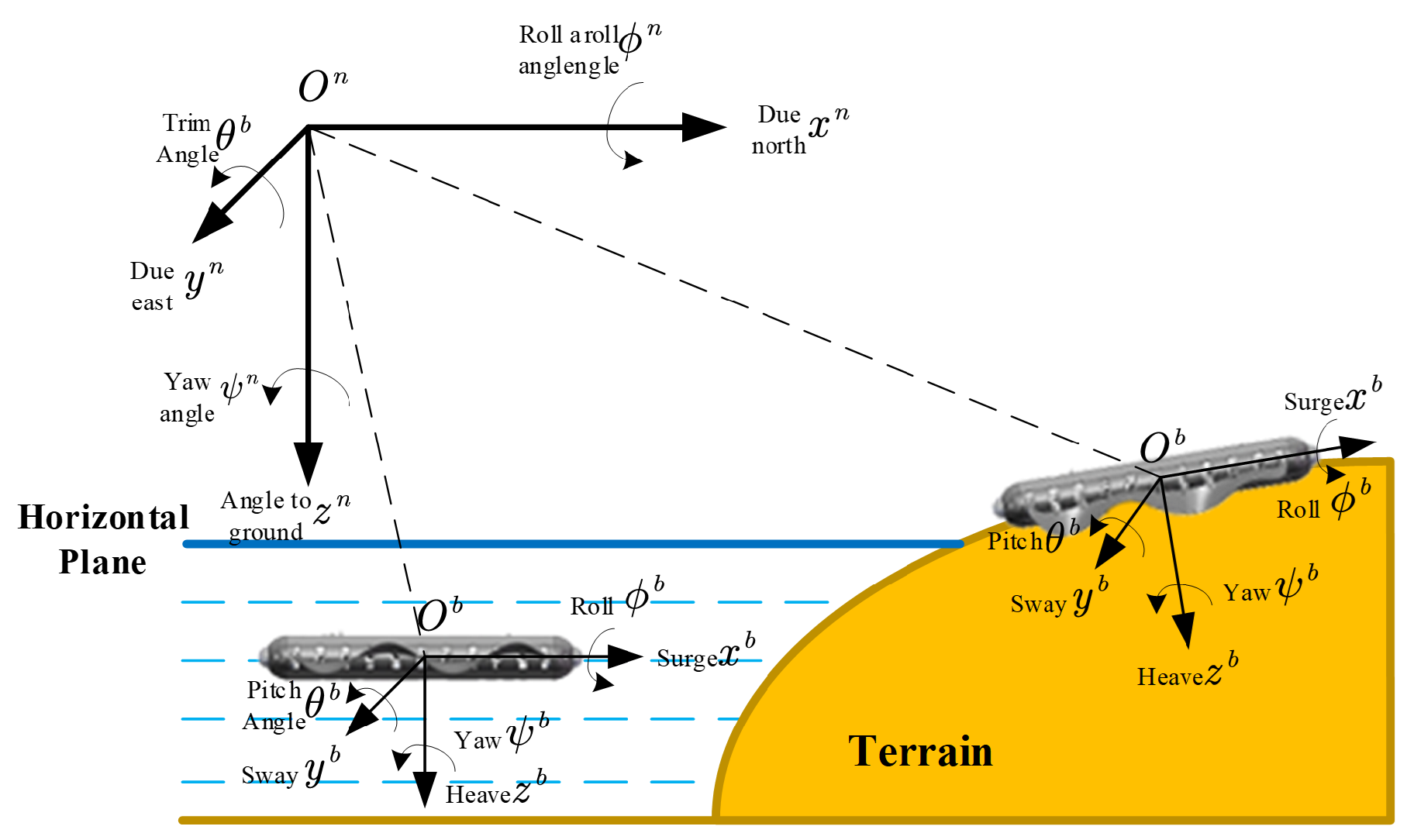
2.1.1. Establishment of Underwater Kinematic Model

In underwater diving mode, the robot operates with five degrees of freedom (5-DOF), as the traverse roll can be neglected. When working on surface water, the lift, traverse roll, and pitch can be neglected, the robot’s motion can be simplified to three degrees of freedom (3-DOF) [31]. To simplify model calculations, the robot’s operations in both modes can be consolidated into a 5-DOF motion model. This approach yields the underwater dynamic equations for amphibious and underwater robots as shown in Equation (4):

$$\left\{\begin{array}{c}\left[\begin{array}{c}\dot{x}\\ \dot{y}\\ \dot{z}\\ \dot{\theta }\\ \dot{\psi }\end{array}\right]=\left[\begin{array}{ccccc}cos\theta cos\psi & -sin\psi & sin\theta cos\psi & 0& 0\\ cos\theta sin\psi & cos\psi & sin\theta sin\psi & 0& 0\\ -sin\theta & 0& cos\theta & 0& 0\\ 0& 0& 0& 1& 0\\ 0& 0& 0& 0& 1/cos\theta \end{array}\right]\left[\begin{array}{c}u\\ v\\ w\\ q\\ r\end{array}\right]\hfill \end{array}\right.$$

(4)

2.1.2. Establishment of Land Kinematic Model

When the amphibious robot operates in amphibious switching and land driving modes, the robot is attached to the land surface, and its motion is similar to that of a land robot as shown in Figure 2. The robot moves across complex terrains with varying inclines and elevations. Thus, based on traditional land robot kinematics and considering the slope and elevation of the terrain, a 3-DOF land kinematic model is established:

$$\left\{\begin{array}{c}\left[\begin{array}{c}\dot{x}\\ \dot{y}\\ \dot{\psi }\end{array}\right]=\left[\begin{array}{ccc}cos\theta cos\psi & -sin\psi & 0\\ cos\theta sin\psi & cos\psi & 0\\ 0& 0& 1/cos\theta \end{array}\right]\left[\begin{array}{c}u\\ v\\ r\end{array}\right]\hfill \\ \left[\begin{array}{c}z\\ \theta \end{array}\right]=\left[\begin{array}{cc}A& B\end{array}\right]\hfill \\ A=\left[\begin{array}{c}{z}_e+h_{robot}cos\theta /2\\ {\theta }_e\end{array}\right]\hfill \\ B=\left[\begin{array}{c}terrai{n}_z(x,y)+h_{robot}cos\left(terrai{n}_{\theta }(x,y)\right)/2\\ terrai{n}_{\theta }(x,y)\end{array}\right]\hfill \end{array}\right.$$

(5)

In the above equation, $z_e$ represents the height of the terrain to which the robot is attached relative to the geodetic coordinate frame, ${\theta }_e$ represents the pitch angle of the terrain to which the robot is attached relative to the geodetic coordinate frame, and they are only related to the horizontal and vertical coordinates $\left(x,y\right)$ of the terrain. $h_{robot}$ represents the height of the robot.

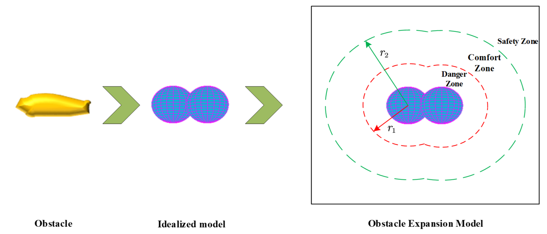
2.2. Obstacle Expansion Model

In the process of local path planning and dynamic obstacle avoidance, it is inevitable to encounter various unknown obstacles [32]. The modeling method of obstacles affects the safety of obstacle avoidance and the complexity of calculation [33]. To reduce computational complexity, obstacles are idealized and modeled as spheres. To enhance obstacle avoidance safety, an obstacle expansion model is established, dividing the area around obstacles into three zones: danger zone, comfort zone, and safety zone. This ensures that the robot maintains a safe distance during motion and avoids collisions. The establishment of idealized obstacle models and the expansion model is illustrated in Figure 3.

As shown in Figure 3, obstacles are first modeled as a combination of multiple spheres, then divided into three regions: a danger zone with a radius of $r_1$, which the robot is prohibited from entering; a comfort zone with a radius of $r_2$, where the robot is allowed to approach slowly; and a safety zone beyond these, where the robot can move freely.

Simplifying the robot’s obstacle avoidance by conceptualizing obstacles as a combination of spheres and uniformly expanding them in all directions reduces the computational load, thereby accelerating the computational speed of local path planning algorithms. Establishing the obstacle expending model and dividing the surrounding areas into risk zones can prevent unintended contact between the robot and obstacles, which can improve the robot’s operational safety. This also serves as the foundation for the improvement of target function and dynamic prediction of obstacles in this paper.

3. Improved Dynamic Window Approach

In order to meet the dynamic obstacle avoidance requirements of amphibious robots in water–land integrated environment, an improved dynamic window approach (IDWA) is proposed to overcome the shortcomings of traditional DWA algorithm, such as high sensitivity of the evaluation parameters, poor dynamic obstacle avoidance ability, and unreachable targets [23,34]. This improvement involves modifying weighting coefficients in the evaluation function and introducing a distance cost function to resolve issues like unreachable targets and the overshooting of endpoints. Additionally, adaptive adjustment of the velocity resolution enhances the algorithm computation speed and the robot’s capability to navigate narrow gaps. Furthermore, a dynamic obstacle prediction approach is introduced to the IDWA, which increases the robot’s safety, flexibility, and foresight.

3.1. Improved Evaluation Function

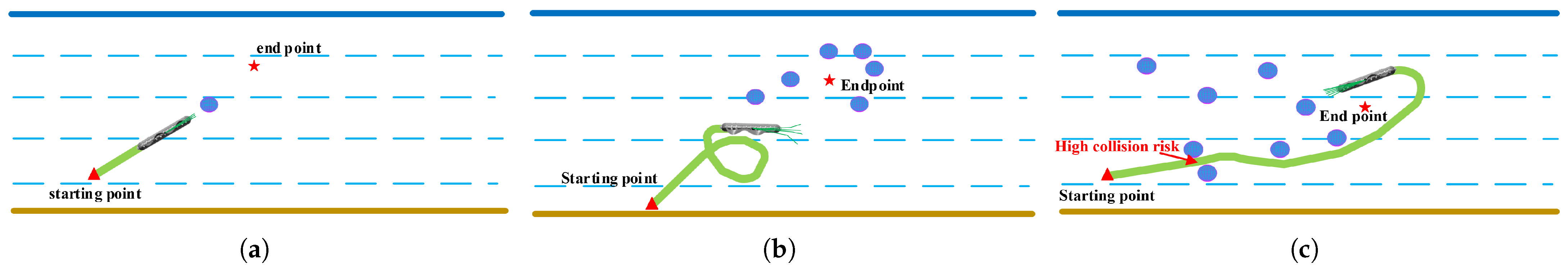
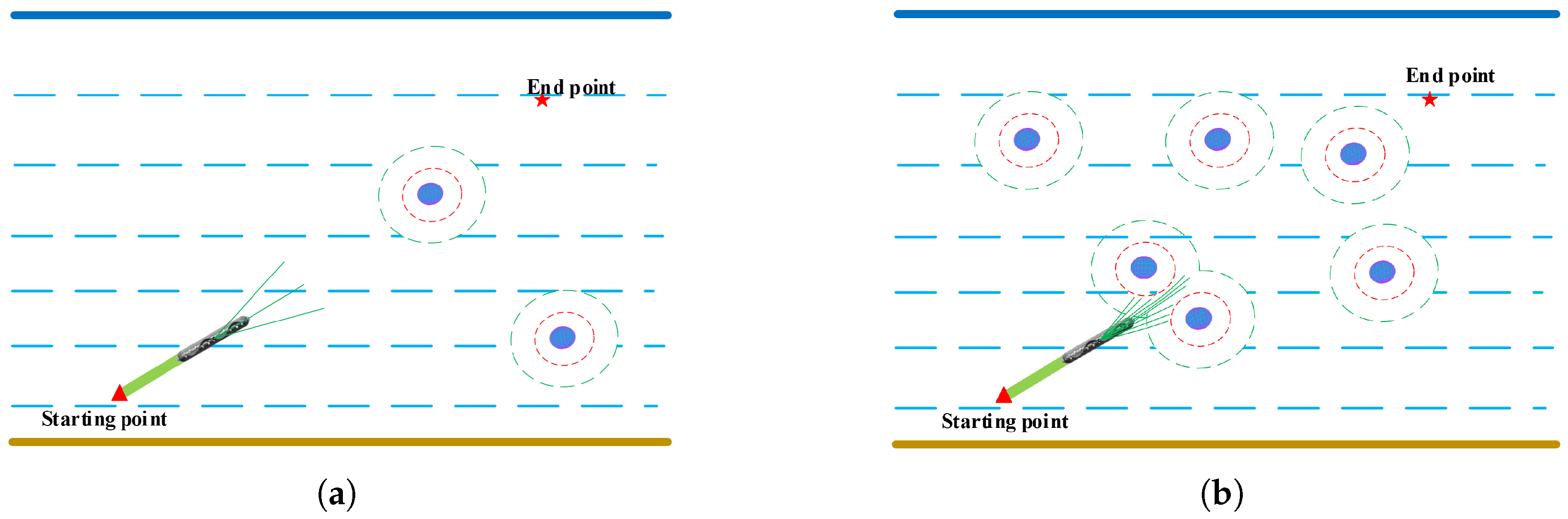
The evaluation factors are fixed and independent in the traditional DWA algorithm. As shown in Figure 4, there are three main shortcomings of the function in water–land environments.

• When the heading factor $\alpha$ is unsuitable, the robot may stop moving forward when approaching obstacles in the path, resulting in an unreachable target.
• When the safety factor $\beta$ is unsuitable, the robot may frequently change direction to avoid obstacles, leading to missing target and even circling.
• When the velocity factor $\gamma$ is unsuitable, the robot may neglect safety while multiple obstacles around the path and may overshoot when approaching the endpoint.

Addressing the issue of an unsuited $\alpha$ value leading to an unreachable target, as illustrated in Figure 4a, this study proposes an improved heading evaluation factor. When the robot is within the comfort zone of an obstacle, the proposed factor decreases with the angular difference between the robot’s heading and the target direction. The improved heading evaluation factor can help the robot to escape from a potential stop status, which is expressed in Equation (6):

$${\alpha }^{*}=\left\{\begin{array}{cc}\alpha \hfill & \mathrm{if}{d}_{romin}>r_2\hfill \\ \alpha \times {\displaystyle \frac{|{\varpi }_{ro}^{*}-{\varpi }_{rg}^{*}|}{180}}\hfill & \mathrm{if}{d}_{romin}\le r_2\hfill \end{array}\right.$$

(6)

where $d_{ro min}$ represents the minimum distance between the robot and the nearest obstacle, $r_2$ represents the radius of the comfort zone in the obstacle expansion model, ${\varpi }_{ro}$ represents the angularity of the heading direction relative to the nearest obstacle, and ${\varpi }_{rg}$ indicates the angularity of the heading direction relative to the target.

An unsuitable $\beta$ value results in circling as illustrated in Figure 4b. This happens because numerous obstacles lie in the target direction, and the DWA safety evaluation function is overweighted. Consequently, even when obstacles are well beyond the safe distance, they still exert a repulsive force on the robot. To resolve this, we adjust the safety evaluation function so that obstacle avoidance is only triggered when the robot is close to obstacles. The improved safety evaluation function, $dis{t}^{*}$, is defined in Equation (7):

$$dis{t}^{*}=\left\{\begin{array}{cc}1\hfill & \mathrm{if}{d}_{ro min}>r_2\hfill \\ {\displaystyle \frac{d_{ro min}-r_1}{r_2-r_1}}\hfill & \mathrm{if}{r}_1<d_{ro min}\le r_2\hfill \\ -\infty \hfill & \mathrm{if}{d}_{ro min}\le r_1\hfill \end{array}\right.$$

(7)

In the above formula, $r_1$ represents the radius of the danger zone in the obstacle expansion model. When the robot is moving within the safe zone, the safety assessment score remains unchanged. In the comfort zone, the robot will encounter a repulsive force from obstacles. And if the predicted position lies within the danger zone, that path will be discarded.

An unsuitable factor $\gamma$ value makes the priority of the speed evaluation function too high, and the algorithm cannot reduce the speed to avoid collisions as shown in Figure 4c. To address this issue, this study refines the velocity evaluation factor ${\gamma }^{*}$; the new factor can reduce the priority level of speed when navigating in changing environments and avoiding obstacles but prioritize the safety of the path. The improved factor is shown in Equation (8):

$${\gamma }^{*}=\left\{\begin{array}{cc}\gamma \hfill & \mathrm{if}{d}_{ro min}\ge r_2\hfill \\ \gamma \times {\displaystyle \frac{d_{ro min}-r_1}{r_2-r_1}}\hfill & \mathrm{if}{d}_{ro min}\le r_2\hfill \end{array}\right.$$

(8)

The overshoot near the endpoint illustrated in Figure 4c is attributed to two factors. Firstly, the velocity factor is overweighted in the overall evaluation. Secondly, the system inadequately considers the distance between the robot and its destination. During the phases of approaching the endpoint, the robot maintains a high speed instead of decelerating appropriately, thus disregarding its nearness to the target. To address this issue, a goal evaluation function, denoted as $goal$, is introduced to evaluate the robot’s distance to the endpoint:

$$\mathrm{goal}=\left\{\begin{array}{cc}0\hfill & \mathrm{if}{d}_{rg}>{\displaystyle \frac{d_{sg}}{10}}\hfill \\ {\displaystyle \frac{d_{sg}-10\times d_{rg}}{d_{sg}}}\hfill & \mathrm{if}{d}_{rg}\le {\displaystyle \frac{d_{sg}}{10}}\hfill \end{array}\right.$$

(9)

In the above equation, $d_{rg}$ represents the distance between the robot and the endpoint, while $d_{sg}$ represents the distance between the start point and the endpoint.

In summary, the improved evaluation function can be shown as

$$G\left(\nu ,\phi \right)=\sigma \left({\alpha }^{*}\times \mathrm{heading}+\beta \times dis{t}^{*}+{\gamma }^{*}\times \mathrm{velocity}+\mu \times \mathrm{goal}\right)$$

(10)

where $\mu$ represents the distance evaluation factor.

3.2. Adaptive Velocity Resolution

Velocity resolution, which represents the sampling density in velocity space, is a key parameter affecting both computational efficiency and path planning accuracy. Figure 5 illustrates the impact of velocity resolution in different environments. When there are fewer obstacles on the path as shown in Figure 5a, a small velocity resolution is sufficient for the robot’s navigational needs, which can reduce the computational load of the path planning system. In contrast, when there are many obstacles on the path as shown in Figure 5b, the navigation system requires a large velocity resolution to work out a more viable path among those obstacles.

In response to this challenge, this study introduces the adaptive velocity resolution (AVR) approach. This approach modifies the velocity resolution dynamically according to the robot’s current obstacle environment. The AVR approach reduces the velocity resolution in areas with sparse obstacles, which can conserve computational resources and expedite decision-making processes. Conversely, when the robot navigates in complex and obstacle-rich environments, the AVR increases the velocity resolution to obtain the optimal path between obstacles and ensure the robot’s safety. The function of AVR can be shown as Equation (11):

$$\Delta V^{*}=\Delta V_{min}+\left(\Delta V_{max}-\Delta V_{min}\right)\times e^{-k\left({\Phi }_d{\Phi }_{\rho }\right)}$$

(11)

In the above equation, $\Delta V_{min}$ and $\Delta V_{max}$ represent the minimum and maximum velocity resolutions respectively. k represents the positive coefficient which can impact the navigation system’s responsiveness. ${\Phi }_d$ and ${\Phi }_{\rho }$ are important parameters, which quantify the impact of obstacle distance and distribution on the velocity resolution. They can be shown as Equation (12):

$$\left\{\begin{array}{cc}\hfill {\Phi }_d& ={\displaystyle \frac{d_{ro min}-r_1}{r_2-r_1}}\hfill \\ \hfill {\Phi }_{\rho }& ={\displaystyle \frac{1}{1+{\rho }_o}}\hfill \end{array}\right.$$

(12)

In this equation, ${\rho }_o$ represents the number of obstacles contained within a $100\times 100\times 100$ grid space centered on the robot.

3.3. Dynamic Obstacle Prediction

The traditional DWA algorithm is designed for static environments where obstacles remain stationary, so its ability to avoid obstacles is limited. This algorithm will fail when the obstacles are moving. Figure 6a illustrates the static avoidance strategy, in which the robot avoids obstacles based on the safety evaluation function. This algorithm gradually increases the distance between the robot and the end point. The robot progressively deviates from its optimal path to the target. In order to improve the adaptability of the algorithm in dynamic obstacle environment, a dynamic obstacle prediction approach based on kinematic model of obstacles is introduced. The improved dynamic window approach (IDWA) can monitor and analyze the trajectory of obstacles in real time and forecast the short-term position of these obstacles so it can reduce collision risks and avoid circling. The strategy of the IDWA with dynamic obstacle prediction is shown in Figure 6b.

The dynamic obstacle prediction approach based on the kinematic model includes the following steps:

• State representation: Define the state vector of the obstacle, including position, linear velocity, and acceleration as shown in Equation (13):

  $$X_{oit}={\left[x_{oit},y_{oit},z_{oit},{\nu }_{xoit},{\nu }_{yoit},{\nu }_{zoit},a_{xoit},a_{yoit},a_{zoit}\right]}^T$$

  (13)
  In the above equation, i represent the obstacle index, t represent the current time step, and $x_o$, $y_o$, and $z_o$ represent the obstacle location. Meanwhile, ${\nu }_{xo}$, ${\nu }_{yo}$, and ${\nu }_{zo}$ represent the linear velocities of the obstacle. $a_{xo}$, $a_{yo}$, and $a_{zo}$ represent the accelerations of the obstacle.
• Location acquisition: The obstacle’s position can be obtained in real time by sensor arrays such as LiDAR, visual cameras, sonar, etc.
• Sliding window processing: A sliding window can be constructed by three consecutive points of the obstacle’s dynamic trajectory. Assuming the obstacle’s motion follows a uniformly accelerated linear pattern within a short period, its current velocity and acceleration are estimated using the difference method as shown in Equation (14):

  $$X_{oit}\left(j\right)={\displaystyle \frac{X_{oit}(j-3)-X_{oit-1}(j-3)}{dt}},j=4,5,6,\dots ,9$$

  (14)
• State estimation: Based on the kinematic model, the position of the obstacle can be predicted at the next time point according to Equation (15):

  $$\left\{\begin{array}{c}{X}_{oit+1}\left(j\right)=X_{oit}\left(j\right)+X_{oit}(j+3)\times dt+0.5\times X_{oit}(j+6)\times {\left(dt\right)}^2\hfill \\ j=1,2,3\hfill \end{array}\right.$$

  (15)
• Dynamic obstacle avoidance: The predicted position of the obstacles at the next time point is the same as that of the obstacle for avoidance. In the IDWA algorithm, the robot performs local path planning and obstacle avoidance with the IDWA.
• Repeat the above steps until the end point is reached.

To comprehensively evaluate the performance of the dynamic obstacle prediction approach, we test the IDWA algorithm under various obstacle movement patterns:

• Linear motion with constant velocity: As shown in

  Table 1. Initial location and speed of obstacles.

  NO.	Initial Location	Direction	Moving Speed (m/s)
  Obstacle 1	$[7,5,-11]$	$[0,0,1]$	0.3
  Obstacle 2	$[10,10,-10]$	$[0,0,1]$	0.4
  Obstacle 3	$[8,10,-8]$	$[0,0,1]$	0.2
  Obstacle 4	$[13,8,-5]$	$[1,1,-1]$	0.5
  Obstacle 5	$[13,12,-8]$	$[1,-1,1]$	0.8
  Obstacle 6	$[18,14,-5]$	$[1,1,1]$	0.1
  Obstacle 7	$[18,13,-7]$	$[1,-1,-1]$	0.3

  , obstacles move in straight lines with different velocities (0.1–0.8 m/s). The IDWA achieves a 98.3.
• Circular motion with varying angular velocity: Obstacles are programmed to move in circular patterns with radii ranging from 2 m to 5 m and angular velocities between 0.1 and 0.3 rad/s. The algorithm demonstrates 95.7.
• Random walk with sudden direction changes: Obstacles were set to change direction randomly every 3–5 s with velocities varying between 0.2a and 0.6 m/s. Despite the unpredictable nature of movement, the IDWA maintains 92.1.
• Group movement with multiple coordinated obstacles: Multiple obstacles (3–5) are programmed to move in coordinated patterns, simulating scenarios like fish schools or vessel groups. The algorithm achieves 90.5.

The experimental results across different movement patterns are summarized in

Table 2. Performance under different obstacle movement patterns.

Movement Pattern	Success Rate (%)	Average Safe Distance (m)	Average Response Time (s)
Linear Motion	98.3	2.5	0.15
Circular Motion	95.7	2.3	0.18
Random Walk	92.1	2.1	0.21
Group Movement	90.5	1.9	0.25

.

The results demonstrate that while the IDWA maintains high performance across all movement patterns, its effectiveness slightly decreases as the complexity of obstacle behavior increases. This is particularly evident in group movement scenarios where multiple obstacles create complex interaction patterns. However, even in the most challenging scenarios, the algorithm maintains a success rate above 90% while keeping safe distances above the minimum required threshold of 1.5 m.

To improve computational efficiency, this dynamic obstacle prediction approach is only triggered when the robot enters the comfort zone of the obstacle. This is not only to ensure enough time and space for effective obstacle avoidance operations but also to maximize the system’s computational efficiency.

4. Experimental Evaluation

This experiment is divided into two steps to validate the efficacy of the local path planning method based on the IDWA in a water–land environment. First, simulation experiments are constructed to validate that the IDWA is effective in three different situations. Second, the experiment is conducted to validate its practicality in a water–land environment based on an amphibious robot we designed in the lake.

4.1. Simulation

Three simulation experiments are designed in the water–land environment to test the IDWA algorithm’s actual performance in solving an amphibious robot’s local path planning problem. The IDWA algorithm is compared with DWA and artificial potential field (APF) methods to validate its improved effectiveness when facing unreachable targets, complex terrains, and moving obstacles. The parameters of the robot are shown in

Table 3. Parameters of the amphibious robot.

Parameter	Value
size of robot (length, width and height) (mm)	$2275\times 780\times 317$
underwater turning radius (mm)	1218
turning radius on land (mm)	1623
crossing ability (mm)	≤430
climbing ability ($\theta$)	≤30°

, and the parameters of the simulation are shown in

Table 4. Parameters of the simulation experiment.

Parameter	Value
map size (m)	$80\times 40\times 20$
radius of danger zone (m)	$1.5$
radius of comfort zone (m)	3
maximum number of iterations $T_{max}$	1000
heading factor $\alpha$	1
safety factor $\beta$	1
velocity factor $\gamma$	1
distance evaluation factor $\mu$	1
linear velocity resolution $\Delta \nu$ (m/s)	$0.1$
angular velocity resolution $\Delta \phi$ (rad/s)	$0.035$
maximum linear velocity underwater/overland $\nu \ast wmax$/$\nu \ast lmax$ (m/s)	$1/0.5$
maximum angular velocity underwater/overland $\phi \ast wmax$/$\phi \ast lmax$ (rad/s)	$0.87/0.52$
maximum linear acceleration underwater/overland $a_{w\nu }$/$a_{l\nu }$ (m/${\mathrm{s}}^2$) (T)	$0.5/0.25$
maximum angular acceleration underwater/overland $a_{w\phi }$/$a_{l\phi }$ (rad/${\mathrm{s}}^2$)	$0.25/0.16$
iteration interval time $dt$ (s)	$0.15$
sliding window time $t_w$ (s)	4
gravitational coefficient $k_a$	$0.1$
expulsive force $k_r$	$0.1$

.

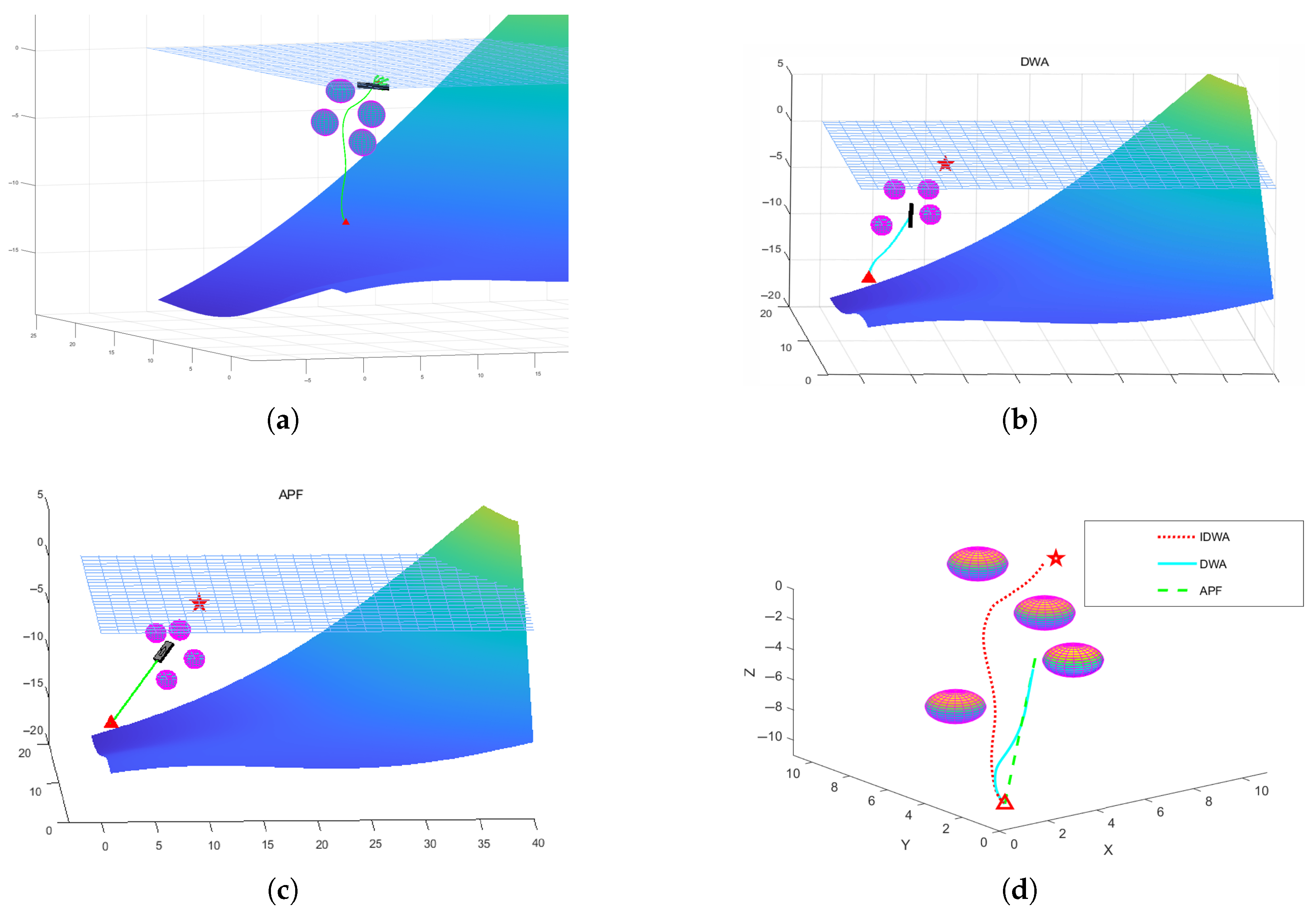
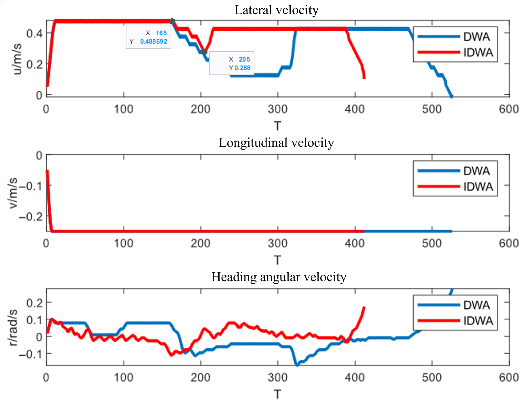
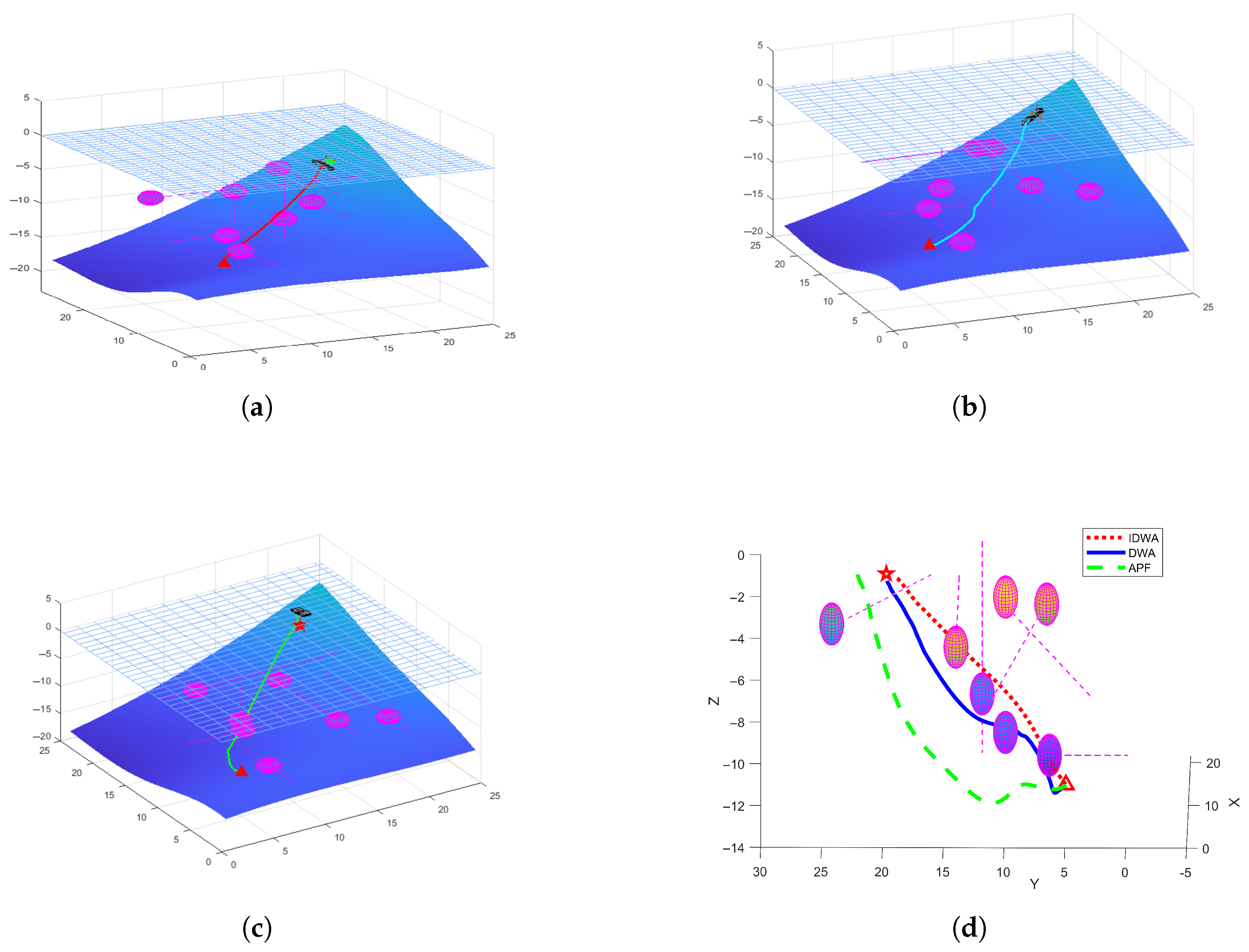
4.1.1. Simulation Experiment for Unreachable Target

This study designs two simulation experiments to validate the IDWA algorithm’s capability to address unreachable target situations in the underwater environment.

In the first experiment, the robot is positioned at an initial state $P_o=\left[1,1,-10,0,\pi /4\right]$. Here, the state vector represents the robot’s initial position in 3D space, where $\left[1,1\right]$ indicates its starting position in the horizontal plane, $-10$ represents a depth of 10 units underwater, 0 denotes the initial velocity, and $\pi /4$ indicates the initial heading angle of 45 degrees. The robot is attempting to move from the starting point $\left[1,1,-10\right]$ to the target point $\left[10,10,-1\right]$, with obstacles located at $\left[8,8,-3;6,6,-1.8;3,7,-1.5;7,10,-2\right]$. These obstacles are strategically positioned along the path: the first obstacle at $\left[8,8,-3\right]$ is placed near the target at a medium depth, the second at $\left[6,6,-1.8\right]$ in the middle of the path at a relatively shallow depth, the third at $\left[3,7,-1.5\right]$ early in the path close to the surface, and the fourth at $\left[7,10,-2\right]$ near the target area at a shallow depth. In this experiment, the local paths are generated by three algorithms (IDWA, DWA, and APF) as shown in Figure 7. The path comparison demonstrates the three algorithms’ distinct responses to obstacles on the path. Furthermore, the linear and angular velocities of IDWA and DWA are compared in Figure 8.

In the second experiment, the robot is positioned at an initial state $P_o=\left[5,35,-15,0,-\pi /4\right]$. Here, the state vector represents the robot’s initial configuration where $\left[5,35\right]$ indicates its starting position in the horizontal plane, $-15$ represents its vertical position, 0 denotes the initial velocity, and $-\pi /4$ indicates the initial heading angle. The robot is attempting to move from the starting point $\left[5,35,-15\right]$ to the target point $\left[20,10,-5\right]$, with obstacles located at $\left[18,8,-3;18,8,-7;23,9,-3;22,9,-7;20,6,-5\right]$. In this experiment, the local paths are generated by three algorithms (IDWA, DWA, and APF) as shown in Figure 9. This comparison highlights the ability of IDWA to optimally adjust velocity when encountering obstacles.

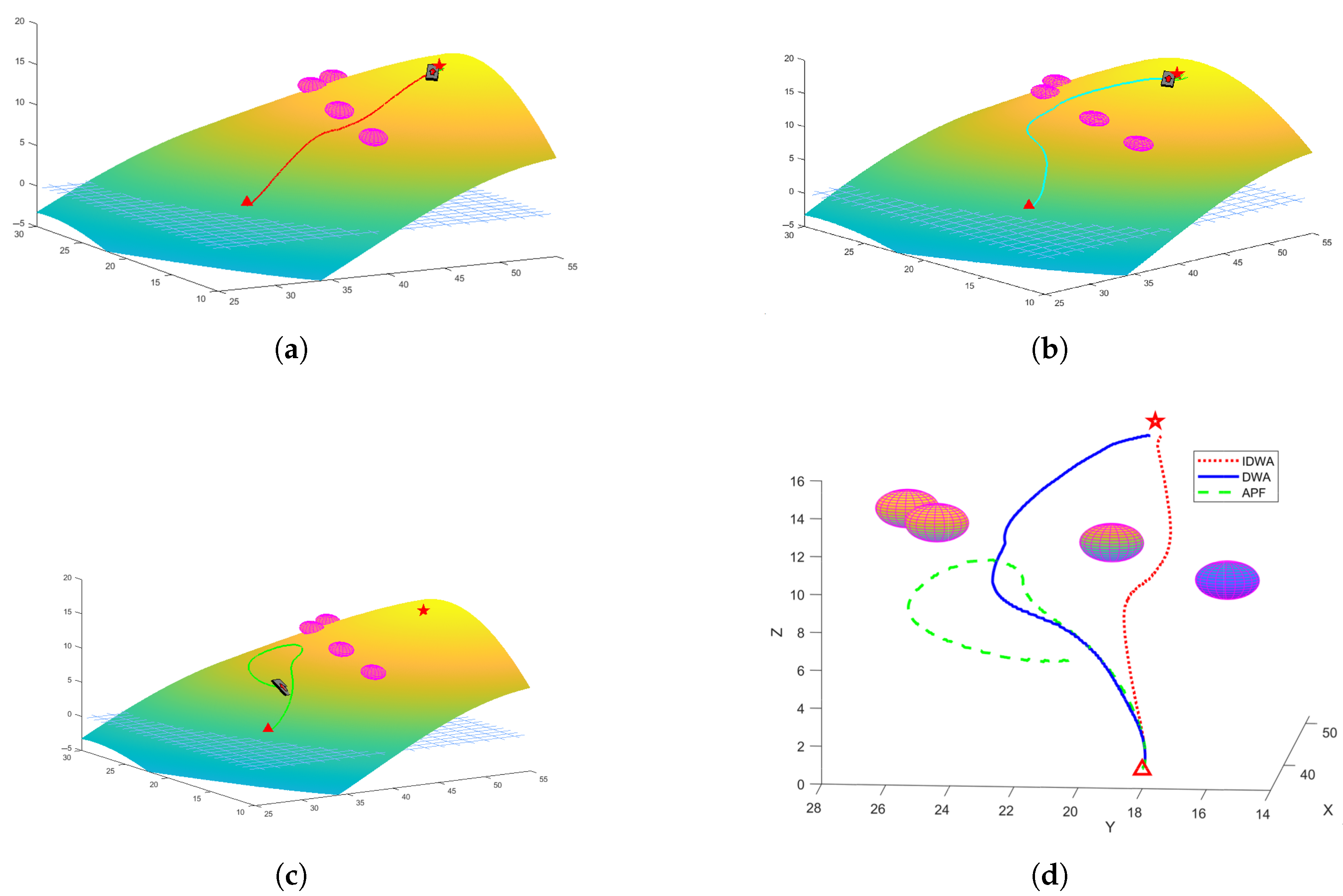
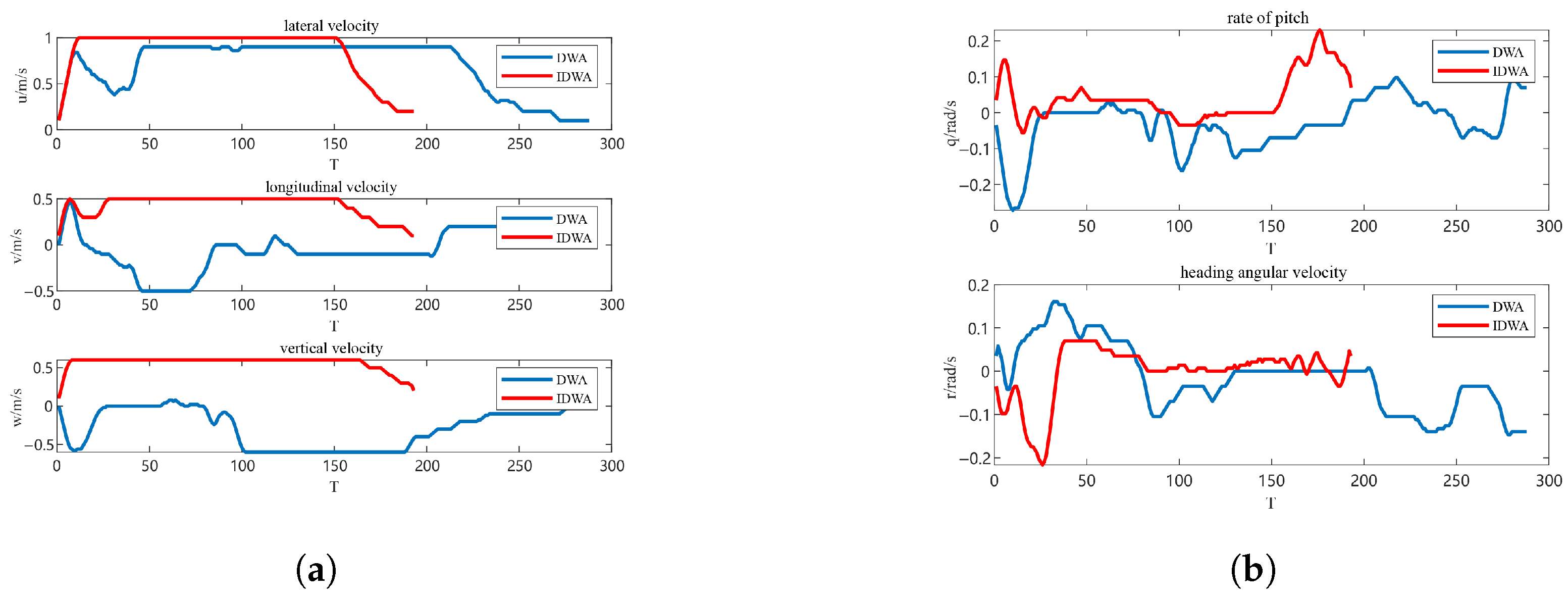
4.1.2. Simulation Experiment for Land Traversal

A simulation experiment for land traversal is designed to validate the obstacle avoidance performance of the IDWA algorithm. As analyzed, the velocity resolution of the DWA algorithm affects both the computational speed and obstacle avoidance precision as shown in Figure 5. In this experiment, when the robot traverses on land, there are multiple obstacles on its path. The starting point is at $\left[34,18,1\right]$, and the endpoint is at $\left[52,19,15.2\right]$. There are several obstacles located at $\left[44,20,10.8;44,17,8.9;46,25,11.3;48,26,11.4\right]$, and the initial robot state is $P_o=\left[34,18,1,0,\pi /6\right]$. The working environment is on land. Figure 10 illustrates the local path planning results for IDWA, DWA, and APF, highlighting the distinction of each path generated by different algorithms when through obstacle-rich environments. The velocity profiles of IDWA and DWA are compared in Figure 11. The ability of the velocity adjustment of IDWA to ensure safe navigation in complex terrains is verified.

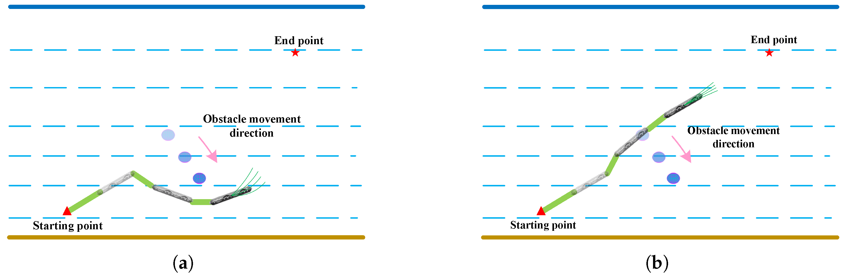
4.1.3. Simulation Experiment for Moving Obstacle

A simulation experiment in underwater is designed to validate the obstacle avoidance performance of the IDWA algorithm in the presence of moving obstacles. As analyzed, when obstacles move at high speeds, the static obstacle avoidance strategy of the DWA increases the risk of collision as shown in Figure 6. In this experiment, multiple moving obstacles are incorporated into the simulation scenario. The starting point is at $\left[5,5,-12\right]$, the endpoint is at $\left[20,20,-5\right]$, and the initial robot state is $P_o=\left[5,5,-12,0,\pi /6\right]$. The working environment is underwater, with obstacle initial coordinates and movement velocities as shown in Table 1. Figure 12 illustrates the local paths generated by the three algorithms, while Figure 13 presents a comparison of the velocity profiles for the IDWA and DWA.

4.1.4. Simulation Results

The results of the simulation experiments for unreachable targets, land traversal, and moving obstacles as shown in

Table 5. Results of simulation experiments.

	Unreachable Target Simulation			Complex Terrain Traversal Simulation			Moving Obstacle Avoidance Simulation
	IDWA	DWA	APF	IDWA	DWA	APF	IDWA	DWA	APF
Completion of tasks	Yes	No	No	Yes	Yes	No	Yes	Yes	Yes
Iteration times	178	500	500	413	526	1000	193	288	251
Task Completion Time (s)	26.7	\	\	61.95	78.9	\	28.95	43.2	37.65
Algorithm Runtime (s)	8.12	21.92	16.07	15.31	22.55	30.29	7.28	11.25	8.88
Path Length (m)	15.85	\	\	26.02	29.89	\	21.61	24.22	27.91

. The target unreachable simulation experiment is shown in Figure 7, Only the IDWA algorithm can successfully navigate around the obstacle and reach the target when the obstacle is on the path from the starting point to the endpoint. The excellent performance of the IDWA is due to the improved evaluation function, which is proposed in Section 3.1. The improved evaluation function reduces the heading factor based on the angular difference between the obstacle and the target when entering the obstacle’s comfort zone. Due to the function, the robot can circumvent the obstacle safely by adjusting its direction. Based on the velocity comparison in Figure 8, the IDWA algorithm demonstrates several advantages over the DWA algorithm. When the robot is far from obstacles during initial local path planning, the IDWA algorithm maintains higher linear velocities. When the robot approaches obstacles, the IDWA responds rapidly with minimal oscillation. Near the end point, the robot exhibits smooth velocity deceleration with negligible overshoot under the IDWA control. As shown in Table 5, the execution time of the IDWA is the shortest among the tested algorithms (IDWA, DWA, and APF), and the path length of the IDWA also closely approximates the Euclidean distance between the start- and endpoints. IDWA can solve the problem of the unreachable target caused by obstacle blockage. Compared with the other two algorithms, the path generated by IDWA is both smoother and shorter.

The performance of the IDWA in the land traversal simulation is shown in Figure 10. According to comparing these results, the performance of the IDWA is the best. The robot that uses the IDWA always moves directly toward the endpoint, and the direction is adjusted when it approaches the danger zone to keep itself safe. The robot moves directly towards the target without interference from obstacles, and the path does not have unnecessary detours or reversals. In the land traversal experiment, the path generated by IDWA is the smoothest and safest among the tested algorithms (IDWA, DWA, and APF) as shown in Figure 12d. The robot begins to slow down when it encounters obstacles at the 165th iteration of the IDWA. When it completes the avoidance maneuver, the robot begins to accelerate at the 205th iteration; the robot returns to its full speed at the 216th iteration as shown in Figure 11. The maximum and minimum heading angular velocities of the IDWA are 0.175 rad/s and −0.112 rad/s, respectively, and the angular velocity variation range is 0.287 rad/s. In contrast, the DWA exhibits maximum and minimum heading angular velocities of 0.165 rad/s and −0.282 rad/s, respectively, with a range of 0.447 rad/s. The heading angular velocity variation of the IDWA is smaller than that of the DWA in the same simulation environment. The path of the IDWA is smother and shorter than that of the DWA. In summary, the IDWA can safely reach the target when there are multiple obstacles on the path in land traversal. The path generated by the IDWA is the shortest and smoothest, and the time taken is the shortest.

The simulation of moving obstacles is shown in Figure 12. When multiple moving obstacles cross the path to the target point, the IDWA algorithm can successfully avoid obstacles and safely reach the target point. The local path is short and smooth. On the contrary, when obstacles approach, the path generated by the DWA and APF algorithms vibrates and circles and even fails path planning. The APF algorithm happens to overshoot near the target point, resulting in circling. By comparing the paths in Figure 12, the path generated by IDWA avoids all obstacles to reach the target point, and the path is smoothest and shortest in the moving obstacles environment. As shown in Figure 13, during the moving obstacles avoidance process, the navigation speed of the IDWA is greater than that of the DWA and even reaches the maximum speed. Compared with DWA, the pitch angle and heading angle changes of the IDWA are reduced by 24.59% and 9.92%, respectively. According to Table 5, the performance of the IDWA is significantly better than that of the DWA and APF; the task completion time of the IDWA is reduced by 32.99% and 23.11%, the algorithm runtime of IDWA is reduced by 35.29% and 18.02%, and the path length of the IDWA is reduced by 10.78% and 22.57%. Through three simulation experiments, the IDWA algorithm can safely avoid various obstacles and reach the endpoint. Its task completion time, runtime, and path length are all the shortest, and the path is smooth without overshooting so that the IDWA can ensure the autonomous navigation capability of amphibious robots in complex water–land environments.

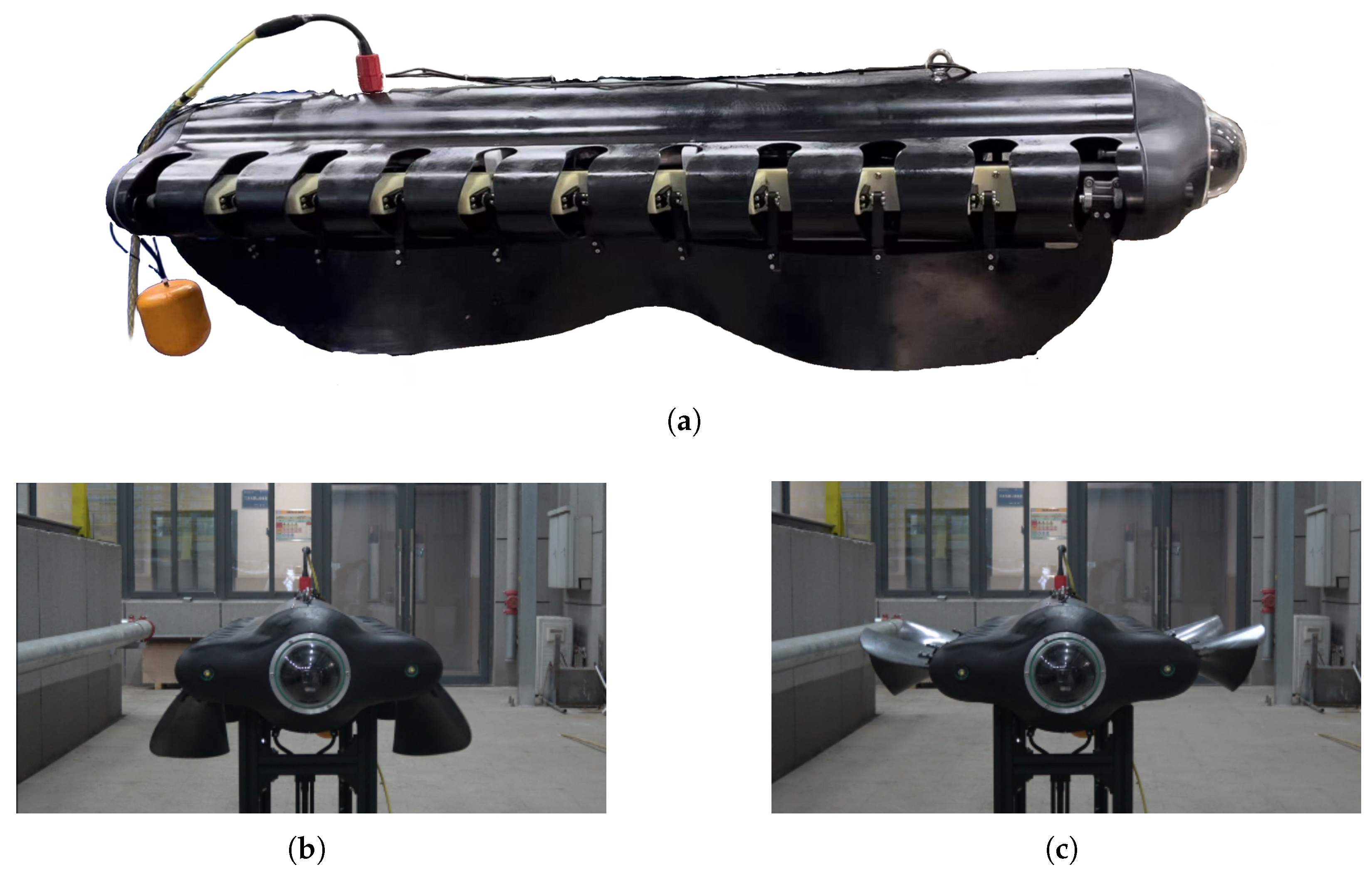
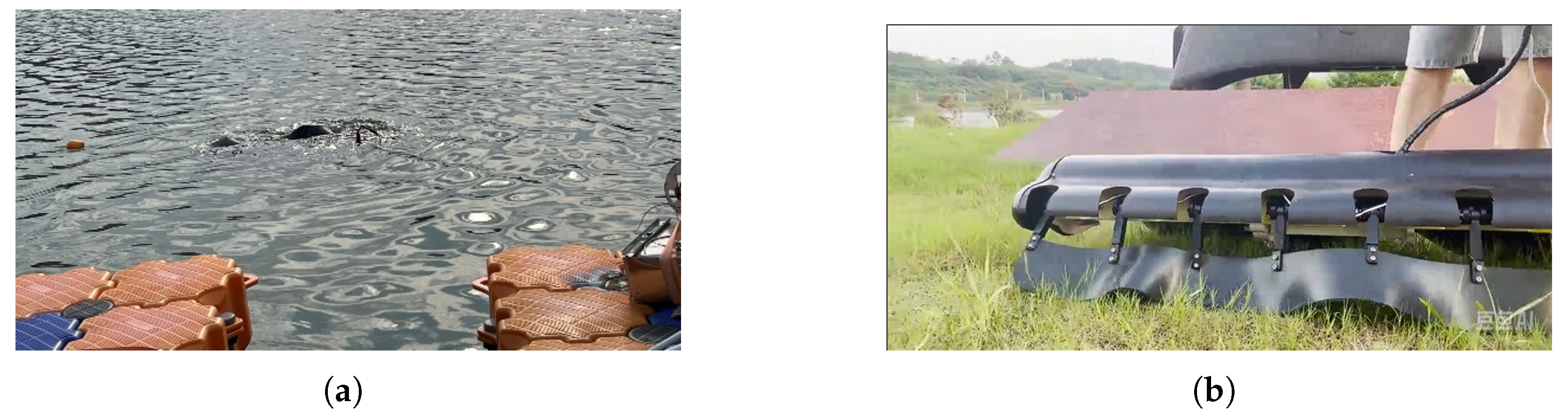
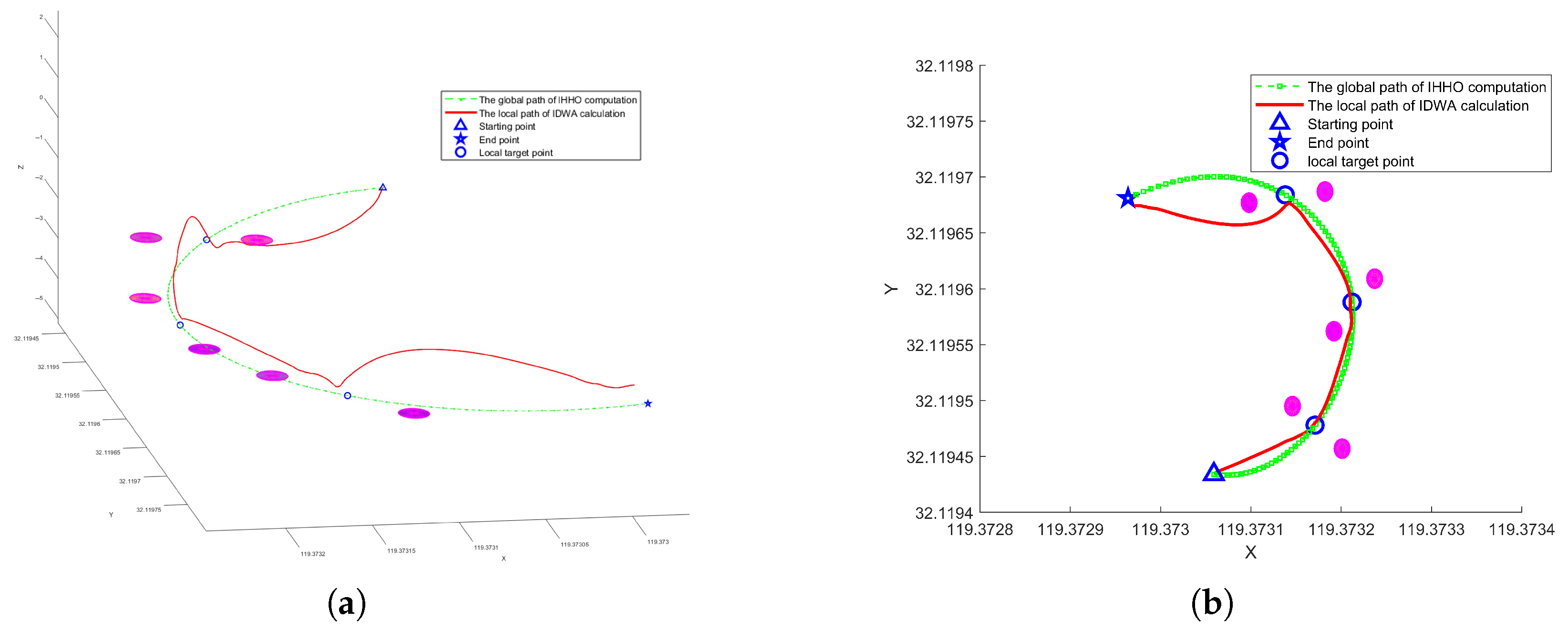
4.2. Lake Experiment

A local path planning experiment was conducted at HAIYUN Lake to validate the availability of the IDWA algorithm. The experimented robot is an amphibious bio-inspired robot modeled after the electric eel as shown in Figure 14. The key specifications of the robot are as follows:

• Drive system:

  -

  Undulating fins actuated by high-torque servos (60 kg $·$ cm) for underwater propulsion.

  -

  Fin-based locomotion generating kinematic wave patterns for various motion modes.

• Sensor suite:

  -

  Navigation system: WTGAHRS2 high-precision inertial navigation system. (Wit-Motion Technology Co., Ltd., Shenzhen, China).

  *

  Integrated JY901B IMU and GPS module.

  *

  Advanced dynamic solving and Kalman filtering algorithms.

  -

  Depth sensor: AS-131 pressure transmitter. (AutoSensor Technologies Co., Ltd., Zhengzhou, China).

  *

  316 L stainless steel isolation diaphragm.

  *

  Temperature-compensated zero point and sensitivity.

  *

  High anti-interference and overload protection.

  -

  Altimeter: ISA500 subsea altimeter (Impact Subsea Ltd., Bridge of Don, Aberdeen, UK).

  *

  500 kHz acoustic signal with digital acoustic technology.

  *

  Integrated attitude and heading measurement.

  -

  Underwater lighting: LM3409-based LED system. (Texas Instruments Inc., Dallas, TX, USA).

  *

  Input voltage: 6–75 V.

  *

  PWM dimming range: 10,000:1.

• Communication:

  -

  E62-DTU (433D30) wireless transmission module. (Chengdu Ebyte Electronic Technology Co., Ltd., Chengdu, China).

  *

  Full-duplex point-to-point transmission.

  *

  1 W transmission power at 433 MHz.

  *

  Frequency hopping spread spectrum (FHSS).

  *

  RS232/RS485 interface support.

The IDWA algorithm is implemented on the main controller with real-time processing capability. The sensor data are collected and processed through an integrated system architecture, ensuring reliable environmental perception and motion control. The implementation maintains stable performance with efficient processing of navigation and control tasks.

The IDWA algorithm is integrated into the robot’s control architecture as follows:

• Sensor data acquisition and processing:

  -

  WTGAHRS2 provides attitude and position data at 100 Hz.

  -

  AS-131 pressure transmitter updates depth information at 10 Hz.

  -

  ISA500 altimeter delivers height measurements at 20 Hz.

  -

  All sensor data are synchronized through the FreeRTOS message queue system.

• State estimation and environment perception:

  -

  Robot pose estimation using Kalman filter fusion of IMU and GPS data.

  -

  Depth calculation using pressure-to-depth conversion ($P=\rho gh$).

  -

  Real-time obstacle detection using sonar and vision data.

  -

  Environmental classification for water–land transition zones.

• Path planning implementation:

  -

  IDWA algorithm runs at 10 Hz planning cycle.

  -

  Dynamic window parameters adjusted based on current motion mode (water–land).

  -

  Obstacle prediction updated at 5 Hz for moving obstacle avoidance.

  -

  Local path segments generated with 0.15 s time step.

• Motion control execution:

  -

  Servo control signals updated at 100 Hz for fin undulation.

  -

  Adaptive gain scheduling for different locomotion modes.

  -

  Smooth transition handling between water and land operations.

  -

  Real-time trajectory tracking with feedback control.

The control system maintains an average processing time of 15 ms per planning cycle, ensuring real-time performance for autonomous navigation. The E62-DTU wireless module enables remote monitoring and parameter adjustment during experiments, with telemetry data transmitted at 10 Hz.

The robot works in the autonomous survey mission in the experiment. The IDWA algorithm is employed to dynamically adjust the robot’s velocity and heading based on local target points in the mission so the robot can successfully circumnavigate all encountered obstacles and attain its designated destination. The process of the autonomous survey mission experiment is shown in Figure 15.

In order to test the obstacle avoidance capability of the IDWA algorithm, the starting point is underwater and the endpoint is on land in this experiment. As shown in

Table 6. Parameters of the lake experiment.

	Longitude	Latitude	Height from Sea Level (m)
Starting Point	119.373284 E	32.119533 N	−2.0
End Point	119.373239 E	32.119601 N	4.0
Local Target Point 1	119.373325 E	32.119549 N	−2.5
Local Target Point 2	119.373335 E	32.119591 N	−3.0
Local Target Point 3	119.373295 E	32.119622 N	−3.5
Virtual Obstacle 1	119.373146 E	32.119495 N	−2.3
Virtual Obstacle 2	119.373201 E	32.119457 N	−2.7
Virtual Obstacle 3	119.373192 E	32.119562 N	−4.0
Virtual Obstacle 4	119.373237 E	32.119609 N	−2.0
Virtual Obstacle 5	119.373182 E	32.119687 N	−2.9
Virtual Obstacle 6	119.373098 E	32.119677 N	−4.1

, three waypoints are selected as local target points, with multiple virtual obstacles with a 1 m radius set up in the path. The global path is loaded into the amphibious robot and navigates it to the starting point. Then, the robot conducts an autonomous survey mission according to the predetermined route. During the process of movement, the robot can successfully bypass obstacles and reach the designated target point smoothly. The algorithm’s local path planning and obstacle avoidance performance are analyzed by the robot’s position, pitch angle, heading angle, and other attitude data, which are read from the robot control system. The robot’s pitch and heading angle changes are illustrated in Figure 16b, and the robot’s path is shown in Figure 17. The experimental results are summarized in

Table 7. Results of the lake experiment.

Path Segment	Length (m)	Time (s)
Start–Local Target Point 1	9.85	14.9
Local Target Point 1–Local Target Point 2	13.23	18.6
Local Target Point 2–Local Target Point 3	12.63	18.0
Local Target Point 3–End	15.59	21.6
Total	51.30	73.1

.

The robot monitoring interface is presented in Figure 16a. The real-time statuses of the robot’s attitude, motion mode, and working environment are displayed in the digital twin area. The environment and obstacles in front of and behind the robot are presented in the monitoring. The real-time identification and labeling of various objects and obstacles are performed using the YOLO3 object detection algorithm. A bird’s-eye view is provided in the map display area. A blue line represents the improved local path planned using the IDWA algorithm. The start point, endpoint, and the robot’s current position are indicated by red, yellow, and black dots, respectively. Virtual obstacles are depicted as red areas.

The robot monitoring interface is presented in Figure 16a. The real-time statuses of the robot’s attitude, motion mode, and working environment are displayed in the digital twin area. The environment and obstacles in front of and behind the robot are presented in the monitoring. The real-time identification and labeling of various objects and obstacles are performed using the YOLO3 object detection algorithm, though the detailed implementation of the vision system is beyond the scope of this paper which focuses on path planning. A bird’s-eye view is provided in the map display area. A blue line represents the improved local path planned using the IDWA algorithm. The start point, endpoint, and the robot’s current position are indicated by red, yellow, and black dots, respectively. Virtual obstacles are depicted as red areas.

The robot’s pitch and heading angle changes are smooth without significant overshoot as shown in Figure 16b. Based on the IDWA algorithm, the robot could avoid all obstacles and navigate safely through waypoints to the endpoint, as demonstrated in Figure 17. The robot maintains an average speed of 0.70 m/s in this complex underwater environment, as indicated in Table 7. This experiment demonstrates that the IDWA can be effectively applied in complex environments. It provides the amphibious robot with great path planning ability and obstacle avoidance performance to reach the designed target.

5. Conclusions

To address challenges in local path planning within complex water–land environments, such as unreachable targets, poor dynamic adaptability, and limited planning range, this study develops a water–land hybrid kinematic model based on traditional kinematic frameworks to suit the water–land environments. In terms of obstacle modeling, this study introduces a sub-region obstacle expansion model to enhance computational efficiency while improving robot safety and movement speed. To address the shortcomings of the traditional DWA algorithm, such as high sensitivity of the parameter evaluation and the poor dynamic obstacle avoidance ability, this study enhances the evaluation function through variable weight coefficients and proposes a distance cost function to address unreachable targets and endpoint overshooting. The Adaptive Speed Resolution can improve the IDWA computation speed and enhance the robot’s ability to pass through narrow gaps. Additionally, the ability to predict dynamic obstacles can optimize the local path and enhance the performance of moving obstacle avoidance simulation, and lake experiments have shown that amphibious robots can operate safely in complex water–land environments by using the IDWA algorithm, whether it is narrow gaps, dense obstacles, or moving obstacles. The IDWA algorithm can reasonably avoid obstacles and safety reach the target point, and the path generated is smooth and shortest. Based on the IDWA algorithm, amphibious robots can perform autonomous detection tasks more efficiently.

Simulation and lake experiments validate that the IDWA improves the robot’s navigation capabilities in complex water–land environments. By using the IDWA, the robot can arrive at the local target more precisely and sooner.

References

1. Xia, M.; Wang, H.; Yin, Q.; Shang, J.; Luo, Z.; Zhu, Q. Design and Mechanics of a Composite Wave-driven Soft Robotic Fin for Biomimetic Amphibious Robot. J. Bionic Eng. 2023, 20, 934–952. [Google Scholar] [CrossRef]
2. Rafeeq, M.; Toha, S.F.; Ahmad, S.; Razib, M.A. Locomotion Strategies for Amphibious Robots—A Review. IEEE Access 2021, 9, 26323–26342. [Google Scholar] [CrossRef]
3. Ding, W.; Zhang, L.; Zhang, G.; Wang, C.; Chai, Y.; Yang, T.; Mao, Z. Research on obstacle avoidance of multi-AUV cluster formation based on virtual structure and artificial potential field method. Comput. Electr. Eng. 2024, 117, 109250. [Google Scholar] [CrossRef]
4. Ohn, S.W.; Namgung, H. Requirements for optimal local route planning of autonomous ships. J. Mar. Sci. Eng. 2022, 11, 17. [Google Scholar] [CrossRef]
5. Zhang, X.; Zhu, T.; Xu, Y.; Liu, H.; Liu, F. Local Path Planning of the Autonomous Vehicle Based on Adaptive Improved RRT Algorithm in Certain Lane Environments. Actuators 2022, 11, 109. [Google Scholar] [CrossRef]
6. Tang, F. Coverage path planning of unmanned surface vehicle based on improved biological inspired neural network. Ocean Eng. 2023, 278, 114354. [Google Scholar] [CrossRef]
7. Xing, T.; Wang, X.; Ding, K.; Ni, K.; Zhou, Q. Improved Artificial Potential Field Algorithm Assisted by Multisource Data for AUV Path Planning. Sensors 2023, 23, 6680. [Google Scholar] [CrossRef] [PubMed]
8. Luo, S.; Zhang, M.; Zhuang, Y.; Ma, C.; Li, Q. A survey of path planning of industrial robots based on rapidly exploring random trees. Front. Neurorobotics 2023, 17, 1268447. [Google Scholar] [CrossRef] [PubMed]
9. Wang, J.; Chi, W.; Li, C.; Wang, C.; Meng, M.Q.H. Neural RRT*: Learning-Based Optimal Path Planning. IEEE Trans. Autom. Sci. Eng. 2020, 17, 1748–1758. [Google Scholar] [CrossRef]
10. Shen, C.; Soh, G.S. Targeted Sampling Dynamic Window Approach: A Path-Aware Dynamic Window Approach Sampling Strategy for Omni-Directional Robots. J. Mech. Robot. 2024, 16, 111001. [Google Scholar] [CrossRef]
11. Kobayashi, M.; Motoi, N. Local Path Planning: Dynamic Window Approach with Virtual Manipulators Considering Dynamic Obstacles. IEEE Access 2022, 10, 17018–17029. [Google Scholar] [CrossRef]
12. Dong, D.; Dong, S.; Zhang, L.; Cai, Y. Path Planning Based on A-Star and Dynamic Window Approach Algorithm for Wild Environment. J. Shanghai Jiaotong Univ. (Sci.) 2024, 29, 725–736. [Google Scholar] [CrossRef]
13. Li, W.; Wang, L.; Fang, D.; Li, Y.; Huang, J. Path planning algorithm combining A* with DWA. Syst. Eng. Electron. 2021, 43, 3694–3702. [Google Scholar]
14. Dai, X. Global existence of solution for multidimensional generalized double dispersion equation. Bound. Value Probl. 2019, 2019, 155. [Google Scholar] [CrossRef]
15. Zhang, X. Path Planning Based on YOLOX and Improved Dynamic Window Approach. In Proceedings of the International Conference on Genetic and Evolutionary Computing, Kaohsiung, Taiwan, 6–8 October 2024; Volume 1145, pp. 26–36. [Google Scholar]
16. Si, M.; Zhou, X.; Zhang, Y. Improvement of Dynamic Window Approach in Dynamic Obstacle Environment. In Proceedings of the Journal of Physics: Conference Series, Hangzhou, China, 30 June–2 July 2023; Voume 2477. [Google Scholar]
17. Yao, M.; Deng, H.; Feng, X.; Li, P.; Li, Y.; Liu, H. Improved dynamic windows approach based on energy consumption management and fuzzy logic control for local path planning of mobile robots. Comput. Ind. Eng. 2024, 187, 109767. [Google Scholar] [CrossRef]
18. Cao, Y.; Mohamad Nor, N. An improved dynamic window approach algorithm for dynamic obstacle avoidance in mobile robot formation. Decis. Anal. J. 2024, 11, 100471. [Google Scholar] [CrossRef]
19. Guo, J.; Huo, X.; Guo, S.; Xu, J. A Path Planning Method for the Spherical Amphibious Robot Based on Improved A-star Algorithm. In Proceedings of the 2021 IEEE International Conference on Mechatronics and Automation (ICMA), Takamatsu, Japan, 8–11 August 2021; pp. 1274–1279. [Google Scholar] [CrossRef]
20. Xiang, L.; Li, X.; Liu, H.; Li, P. Parameter Fuzzy Self-Adaptive Dynamic Window Approach for Local Path Planning of Wheeled Robot. IEEE Open J. Intell. Transp. Syst. 2022, 3, 1–6. [Google Scholar] [CrossRef]
21. Dobrevski, M.; Skočaj, D. Dynamic Adaptive Dynamic Window Approach. IEEE Trans. Robot. 2024, 40, 3068–3081. [Google Scholar] [CrossRef]
22. Hang, P.; Yan, Y.; Fu, X.; Chen, H.; Liu, Y. Research on local path planning of intelligent vehicle based on improved dynamic window approach. In Proceedings of the Third International Conference on Artificial Intelligence and Computer Engineering (ICAICE 2022), Wuhan, China, 11–13 November 2023; Volume 12610. [Google Scholar]
23. Dai, X.; Xu, H.; Ma, H.; Ding, J.; Lai, Q. Dual closed loop AUV trajectory tracking control based on finite time and state observer. Math. Biosci. Eng. 2022, 19, 11086–11113. [Google Scholar] [CrossRef]
24. Wang, R.; Wang, S.; Wang, Y.; Tang, C. Path following for a biomimetic underwater vehicle based on ADRC. In Proceedings of the 2017 IEEE International Conference on Robotics and Automation (ICRA), Singapore, 29 May–3 June 2017; pp. 3519–3524. [Google Scholar] [CrossRef]
25. Xiaoqiang, D.; Wenke, L. Non-global solution for visco-elastic dynamical system with nonlinear source term in control problem. Electron. Res. Arch. 2021, 29, 4087–4098. [Google Scholar]
26. Wang, S.; Wang, Y.; Wei, Q.; Tan, M.; Yu, J. A Bio-Inspired Robot With Undulatory Fins and Its Control Methods. IEEE/ASME Trans. Mechatron. 2017, 22, 206–216. [Google Scholar] [CrossRef]
27. Namgung, H. Local route planning for collision avoidance of maritime autonomous surface ships in compliance with COLREGs rules. Sustainability 2021, 14, 198. [Google Scholar] [CrossRef]
28. Dai, X.; Han, J.; Lin, Q.; Tian, X. Anomalous pseudo-parabolic Kirchhoff-type dynamical model. Adv. Nonlinear Anal. 2022, 11, 503–534. [Google Scholar] [CrossRef]
29. Fossen, T.I. Handbook of Marine Craft Hydrodynamics and Motion Control; John Wiley & Sons: Hoboken, NJ, USA, 2011. [Google Scholar]
30. Fossen, T.I.; Pettersen, K.Y.; Galeazzi, R. Line-of-sight path following for dubins paths with adaptive sideslip compensation of drift forces. IEEE Trans. Control Syst. Technol. 2015, 23, 820–827. [Google Scholar] [CrossRef]
31. Yang, J.; Sacks, E. RRT path planner with 3DOF local planner. In Proceedings of the 2006 IEEE International Conference on Robotics and Automation, Orlando, FL, USA, 15–19 May 2006; Volume 2006, pp. 145–149. [Google Scholar]
32. Hu, Z.; Wang, X.; Zhang, J. Research on Dynamic Obstacle Avoidance Method of Mobile Robot based on Improved A* Algorithm and Dynamic Window Method. Eng. Lett. 2024, 32, 520–530. [Google Scholar]
33. Zhu, X.; Yin, D.; Tang, J. A New Algorithm of Path Planning Based on Dynamic Window Approach. In Proceedings of the 2022 4th International Conference on Robotics, Intelligent Control and Artificial Intelligence, Guangzhou, China, 2–4 December 2022; pp. 1322–1326. [Google Scholar]
34. Li, Y.; Zhu, Q. Local path planning based on improved dynamic window approach. In Proceedings of the 2021 40th Chinese Control Conference (CCC), Shanghai, China, 26–28 July 2021; IEEE: Piscataway, NJ, USA, 2021; pp. 4291–4295. [Google Scholar]
Figure 1. Relationship between geodetic and body coordinate frames.
Jmse 13 00399 g001
Figure 2. The robot moving on land.
Jmse 13 00399 g002
Figure 3. The expansion model of obstacles.
Jmse 13 00399 g003
Figure 4. Shortcomings of the traditional DWA algorithm: (a) Unsuitable α leading to unreachable target. (b) Unsuitable β leading to circling. (c) Unsuitable γ leading to collisions or overshooting.
Jmse 13 00399 g004
Figure 5. Impact of velocity resolution in different environments: (a) small velocity resolution in sparse obstacle environment. (b) large velocity resolution in dense obstacle environment.
Jmse 13 00399 g005
Figure 6. The strategy of IDWA with dynamic obstacle prediction. (a) The strategy of DWA static obstacle avoidance. (b) The strategy of IDWA with dynamic obstacle prediction.
Jmse 13 00399 g006
Figure 7. The path comparison of the unreachable target experiment. (a) Local path of IDWA. (b) Local path of DWA. (c) Local path of APF. (d) Path comparison.
Jmse 13 00399 g007
Figure 8. The velocity comparison of the unreachable target experiment: (a) Comparison of linear velocity. (b) Comparison of angular velocity.
Jmse 13 00399 g008
Figure 9. The path comparison of the unreachable target experiment. (a) Local path of IDWA. (b) Local path of DWA. (c) Local path of APF. (d) Path comparison.
Jmse 13 00399 g009
Figure 10. Path comparison of complex terrain traversal experiment: (a) Local path of IDWA. (b) Local path of DWA. (c) Local path of APF. (d) Path comparison.
Jmse 13 00399 g010
Figure 11. The velocity comparison of land traversal experiment.
Jmse 13 00399 g011
Figure 12. The path comparison of moving obstacle experiment: (a) Local path of IDWA. (b) Local path of DWA. (c) Local path of APF. (d) Path comparison.
Jmse 13 00399 g012
Figure 13. The velocity comparison of moving obstacle avoidance: (a) Comparison of the linear velocity of the IDWA. (b) Comparison of the angular velocity of the IDWA.
Jmse 13 00399 g013
Figure 14. The amphibious mimetic electric eel robot: (a) Side view. (b) On-land mode. (c) Underwater mode.
Jmse 13 00399 g014
Figure 15. The process of the autonomous survey mission experiment: (a) Robot moving in lake. (b) Robot slithering on land.
Jmse 13 00399 g015
Figure 16. Visual monitoring and attitude measurement results of the underwater robot’s lake experiments: (a) The monitoring interface of the robot in the lake experiment. (b) The pitch and heading angle of the robot in the lake experiment.
Jmse 13 00399 g016
Figure 17. The path of the robot in the experiment: (a) Front view. (b) Bird’s-eye view.
Jmse 13 00399 g017