The preceding article calculated the hydrodynamic characteristics of the AUV by applying the spatially constrained motion method. However, for the fully appended model of the AUV, due to cost constraints, there is a lack of comprehensive and precise experimental data on hydrodynamic coefficients to directly validate the accuracy of this calculation method. To address this deficiency, this section proposes utilizing a kinematic and dynamic model based on the existing hydrodynamic coefficients of the AUV, first conducting open-loop control simulations and experiments to preliminarily assess the response characteristics of the AUV. Subsequently, when the MPC method is introduced for closed-loop control simulation and experimentation of AUVs, insufficient accuracy in the hydrodynamic coefficients adopted by the model will directly impact the effective implementation of the MPC control strategy, potentially leading to the unsuccessful application of the MPC method or failure to achieve the desired control effects. If the control accuracy falls within an acceptable range, it indicates that the preceding hydrodynamic calculations possess a certain degree of accuracy.
4.1. Open-Loop Control Simulation and Experimentation for AUV
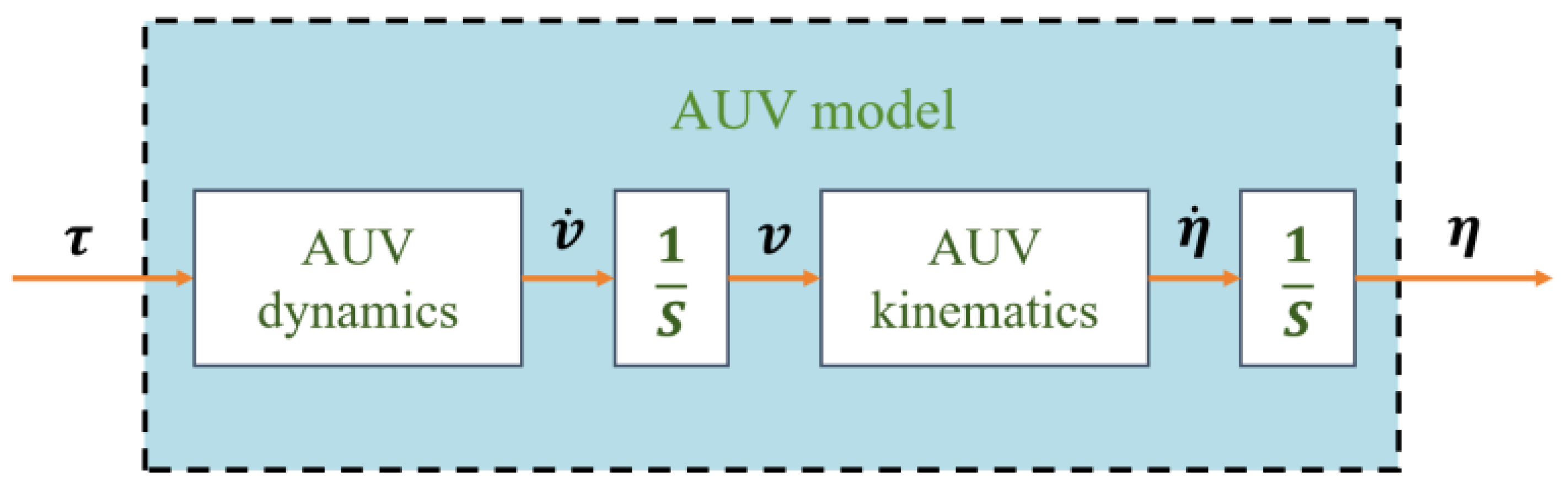
The dynamic model of the AUV is based on the six-degree-of-freedom spatial motion equations and has undergone a simplification process for the hydrodynamic coefficients, resulting in the simplified equations presented below:
The kinematic relationships of the AUV are as follows:
When conducting an open-loop simulation, the dynamic state of the system is denoted as
, the kinematic state is denoted as
, and the system input is denoted as
. When different values of
are applied, different kinematic states are obtained. The schematic diagram of the open-loop control is shown in the following
Figure 12 below.
The AUV studied employs a vector thruster as its propulsion unit. The thrust magnitude T of this thruster is adjustable within the range of [0, 112N], while the angles used to adjust the thrust direction encompass two dimensions:
ranging from [−20°, 20°] and
ranging from [−90°, 90°].
and
control the AUV’s motion in the vertical and horizontal planes, respectively. For a more detailed explanation of these parameters, please refer to reference [
28].
During simulation analysis, the thrust magnitude T is directly used as an input parameter for the simulation model. However, in actual experimental procedures, due to the difficulty in accurately measuring the true thrust magnitude of the thruster directly, the power of the thruster is chosen as the control input parameter. Furthermore, open-water tests on the vector thruster have been conducted in reference [
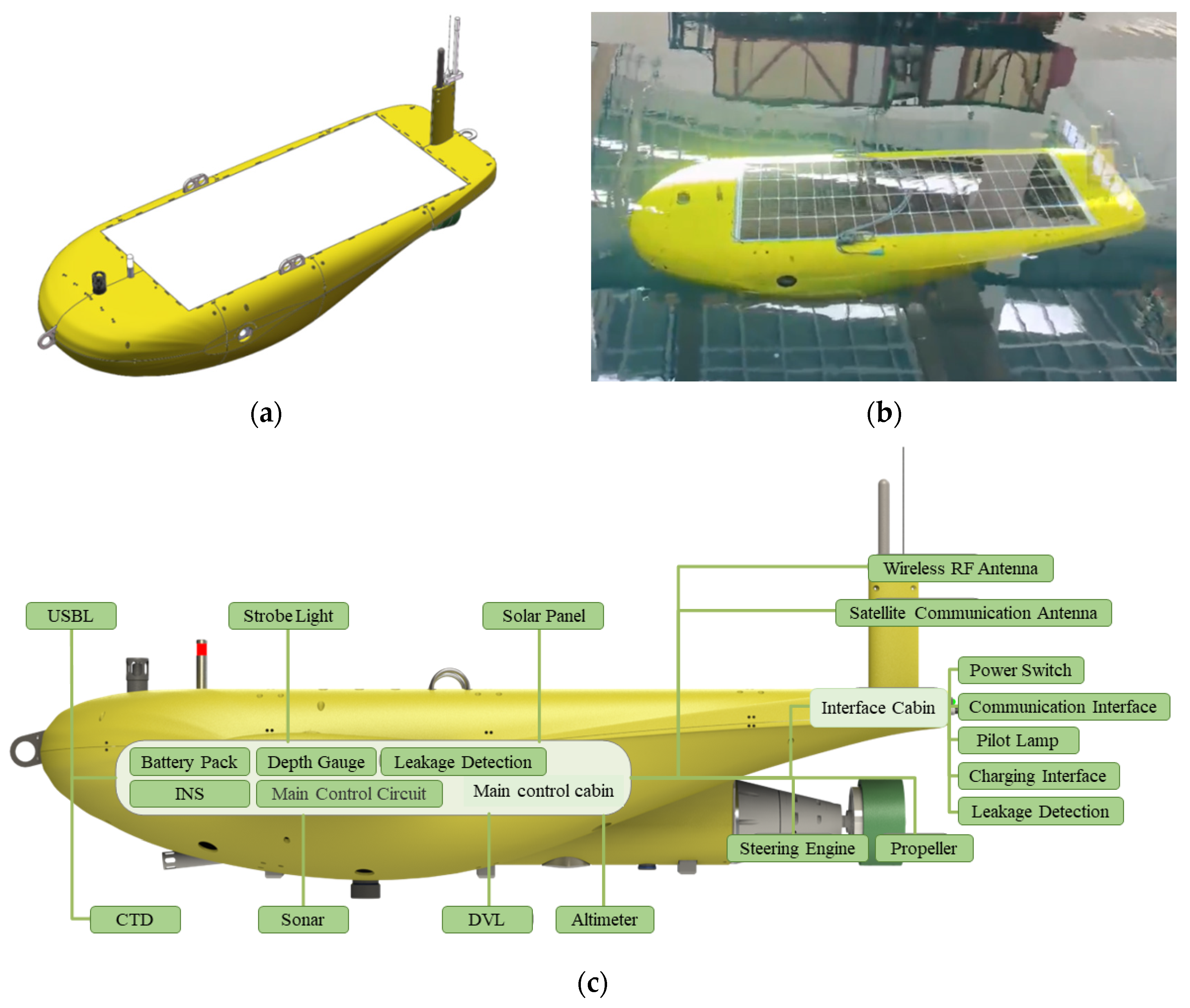
28], establishing a corresponding relationship between power and thrust in still-water conditions, which provides an important basis for the control strategy during experiments. The AUV is an underactuated system capable of controlling state variables such as velocity
, yaw angle
, and pitch angle
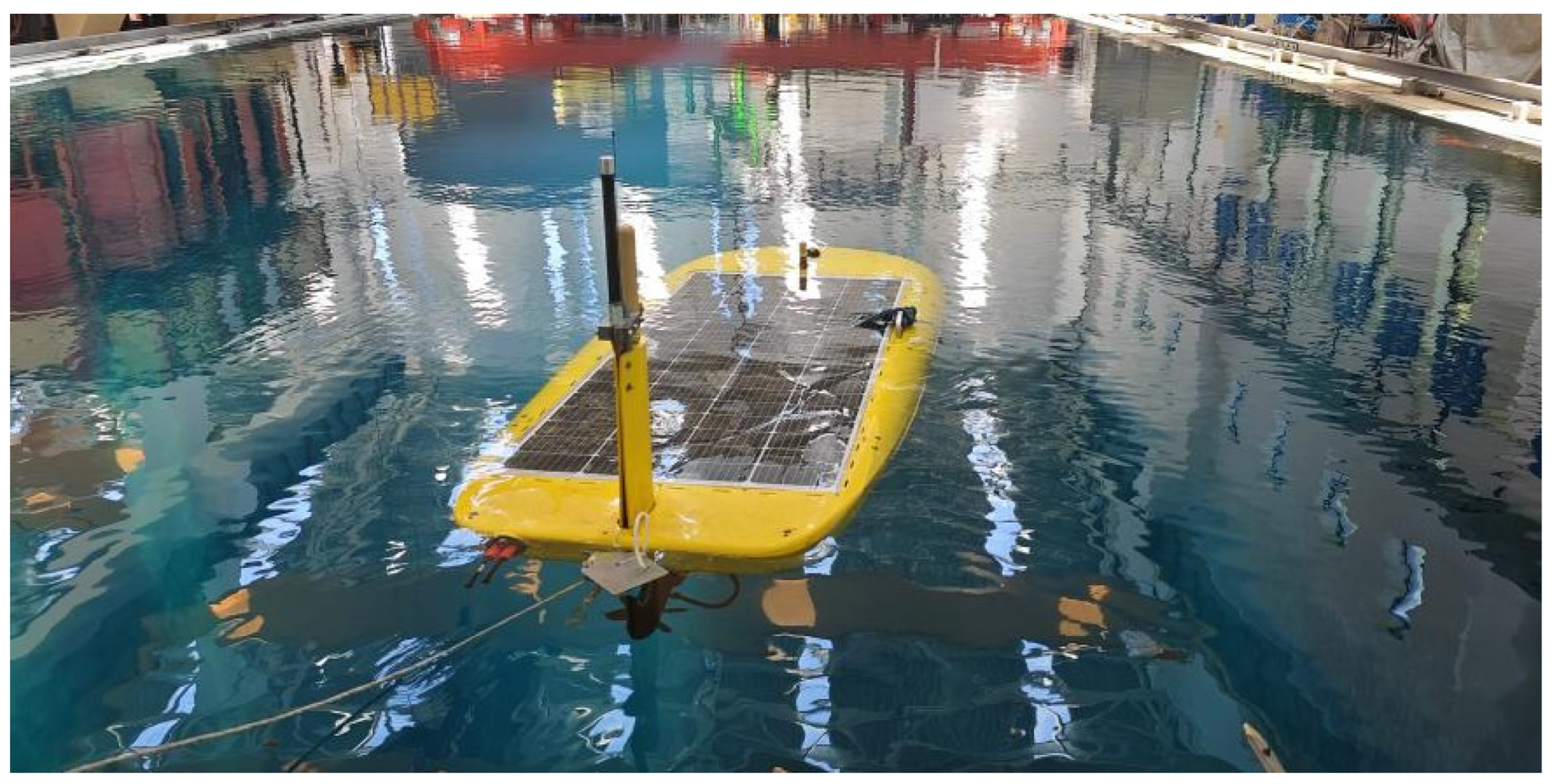
. Both the water tank testing environment and the simulation and experimentation results are illustrated in
Figure 13 and
Figure 14 below.
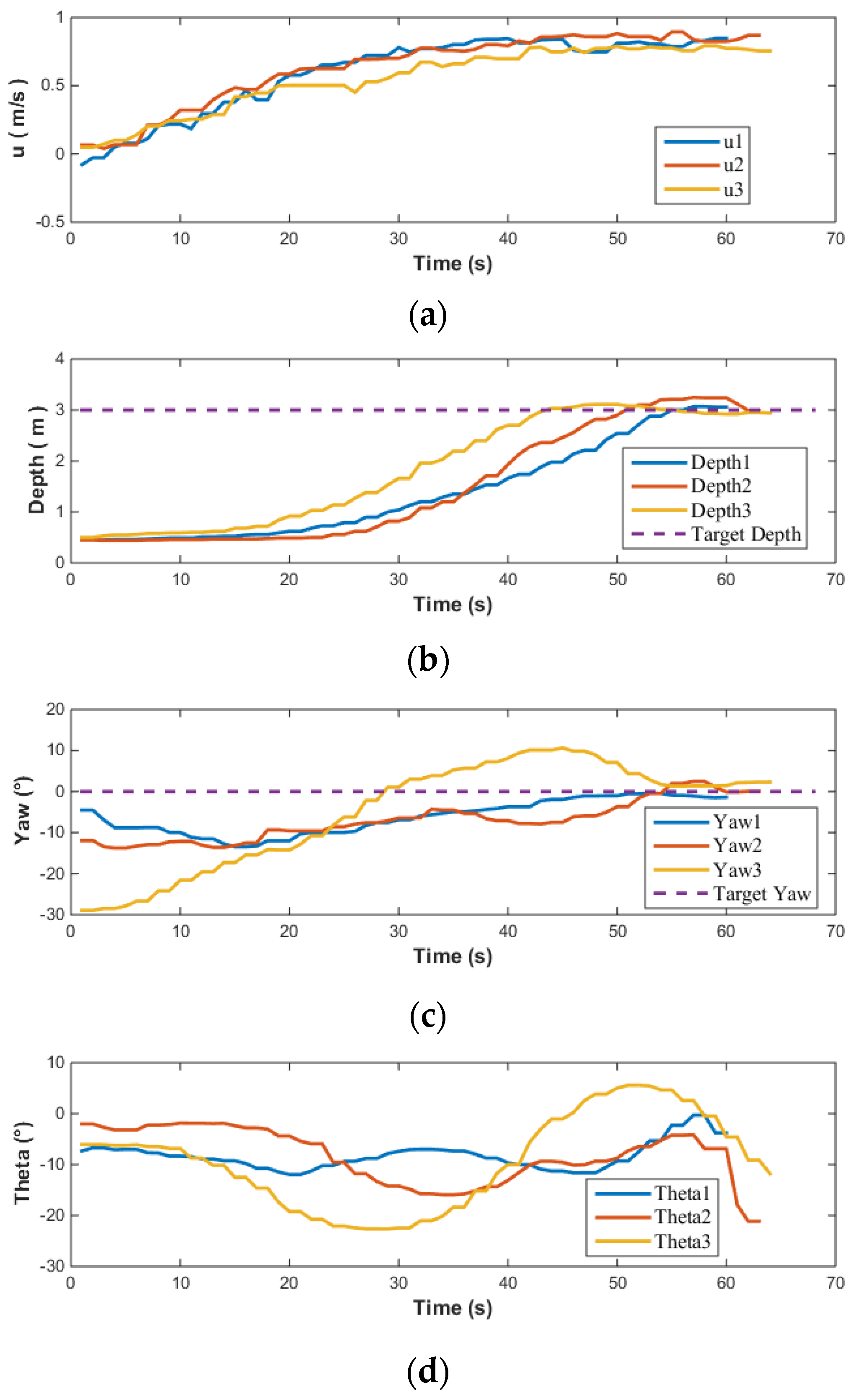
When the system input is , the changes in velocity u during two separate trials and simulations are presented. The maximum velocity achieved by the AUV is 0.9 m/s; however, the simulated acceleration exceeds that observed in both experimental trials. This indicates the presence of certain errors in the hydrodynamic coefficients .
When the system input is , the changes in the heading (yaw angle) during two separate trials and simulations are presented. The results from the experiments and simulations are relatively close, which suggests that the relevant hydrodynamic coefficients possess a certain degree of accuracy.
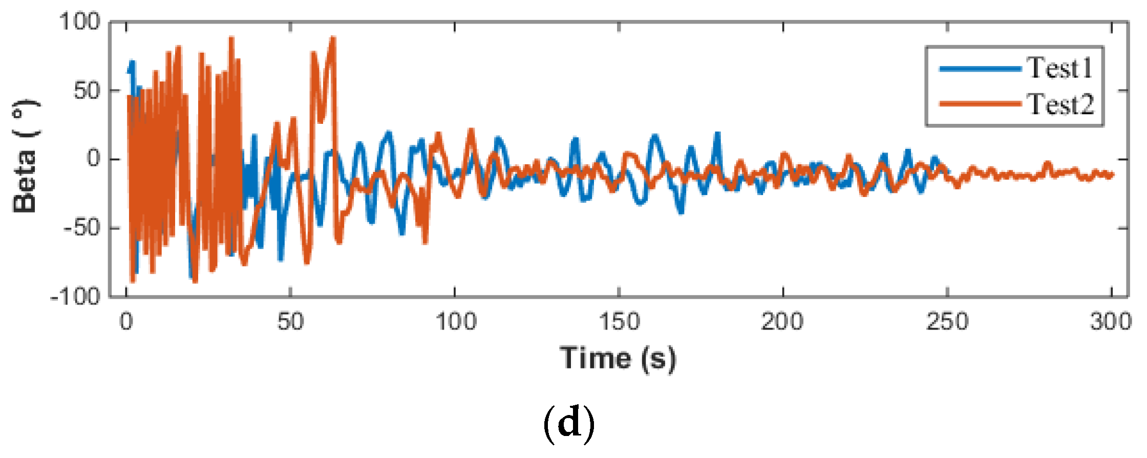
When the system input is , the variations in the pitch angle during two separate trials and simulations are shown. There is a significant error between the experimental and simulation results. The AUV has a negative-lift shape, which exhibits poor structural symmetry. Compared to the calculation of other hydrodynamic coefficients, the calculation error for the hydrodynamic coefficients related to pitch motion is larger.
In summary, by comparing the results of the open-loop control experiments with simulations, the accuracy of hydrodynamic coefficients can be approximately estimated. The consistency between the AUV simulation results and the open-loop control experiments in some data validates that the hydrodynamic coefficients calculated earlier possess certain referential values. However, for those hydrodynamic coefficients with larger errors, it is imperative to explore and consider other effective error compensation methods when designing the closed-loop controller to ensure the precision and stability of the system control.
4.2. MPC Simulation and Experimentation for AUV
In order to reduce the errors introduced by model linearization and decoupling, the MPC controller designed in this section is constructed directly based on the nonlinear six-degree-of-freedom dynamic Equations (22)–(27). The system state of the AUV is denoted as
, and the system input is
. From the above equation, the general expression of the AUV can be derived as:
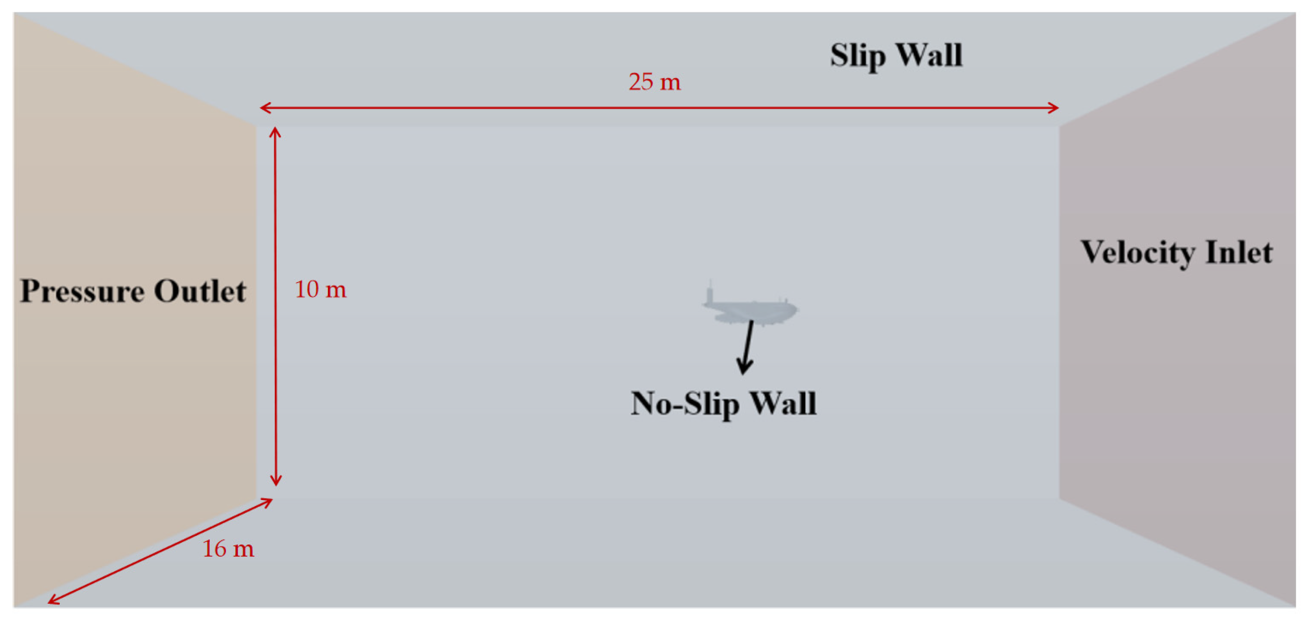
Generally, MPC is used for trajectory tracking control of AUVs. In this paper, to verify the accuracy of the hydrodynamic coefficients, the validation of the AUV is conducted in an undisturbed indoor pool. Due to the limited test site, the speed control, depth control, and yaw control of the AUV are verified in the pool. Based on the above equation, the MPC formula for AUV motion control can be established as follows:
In the above equation,
represents the cost function. And
denotes the error state cost, which can be adjusted according to the state variables that need to be controlled.
is the terminal cost function. Typically, for an underactuated AUV performing simultaneous speed control, depth control, and yaw control, the error state cost at this time is:
For the practical application of the algorithm, there may be a situation where the computing power of the MCU is insufficient, requiring the simplification of the error state cost to improve computational efficiency. In this case, when only depth control and heading control are performed, the error state cost is as follows:
For depth control of an underactuated AUV, it is common to first control the pitch angle and then indirectly control the depth. In this scenario, the error state cost is:
where
,
,
, and
are the target speed, target depth, and target yaw, respectively.
,
, and
are the predicted speed, predicted depth, and predicted yaw of the AUV under the predicted input
.
is the speed error,
is the depth error,
is the yaw error.
represents the control error.
is the weight coefficient for the velocity control performance index,
is the weight coefficient for the pitch angle control,
is the weight coefficient for the heading angle control,
is the weight coefficient for the depth control, and
is the weight coefficient for the control input.
To derive the terminal cost function, the system model
needs to be linearized, resulting in an approximate linearized model as follows:
where
,
. Solve the Riccati equation to obtain
.
Determine the local linear stabilizing feedback gain
for the system.
Given
,
, solve the Riccati equation to obtain
.
Obtain the terminal cost function.
where
,
is a K function, which is defined as follows:
The K function, denoted as
:
(
is defined as a positive real number), is a continuous and strictly increasing function, with the property that
.
where
, the defined minimum value
is denoted as
, and the corresponding optimal input sequence is denoted as
.
The optimal state prediction trajectory
corresponding to u* is denoted as:
When the system transitions to the next state,
, there is a control law that governs this transition.
satisfies the following conditions:
where
At this time, the performance index
corresponding to the control rate (or control law) satisfies:
Therefore, it can be obtained as follows:
Let
be a Lyapunov function. When the rolling horizon control law is
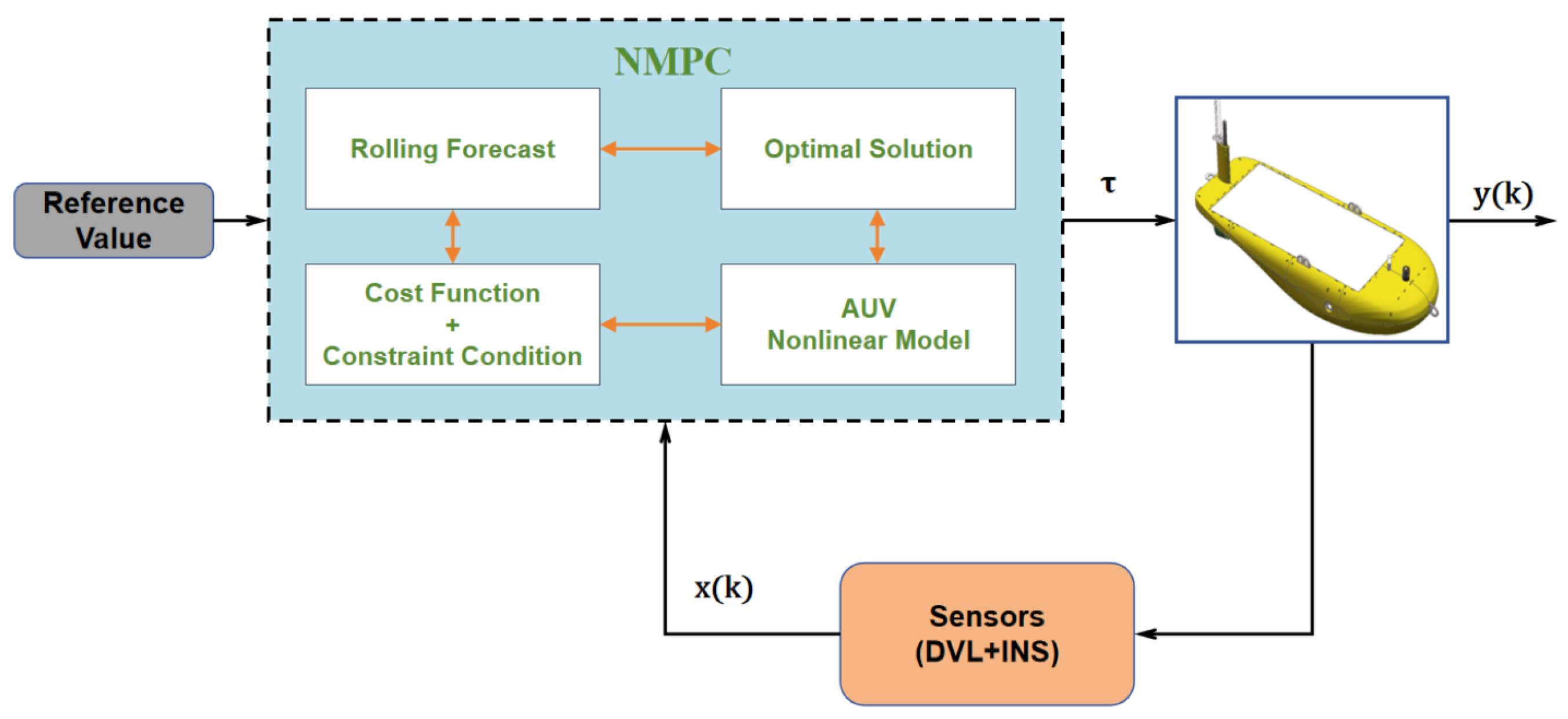
, the system is stable. The main principle of MPC is illustrated in
Figure 15 below:
Since the MCU used by the AUV is a Raspberry Pi 4B, which has limited computing power, it is necessary to pre-determine some suitable test parameters through simulation before conducting actual tests. Additionally, other test parameters need to be determined based on the physical constraints of the AUV, such as the angle adjustment speed of the vector thrusters, sampling frequency, and execution frequency.
When the underactuated AUV performs simultaneous speed control, depth control, and yaw control, the error state cost is denoted as
, with weight coefficients
,
,
,
, and U = 1 m/s,
,
m,
. The prediction horizon
is set to 8 and 16, respectively, for these simulations. When the underactuated AUV performs only depth control and yaw control, the error state cost
is calculated with the same weight coefficients
,
,
, and
m,
. The prediction horizon
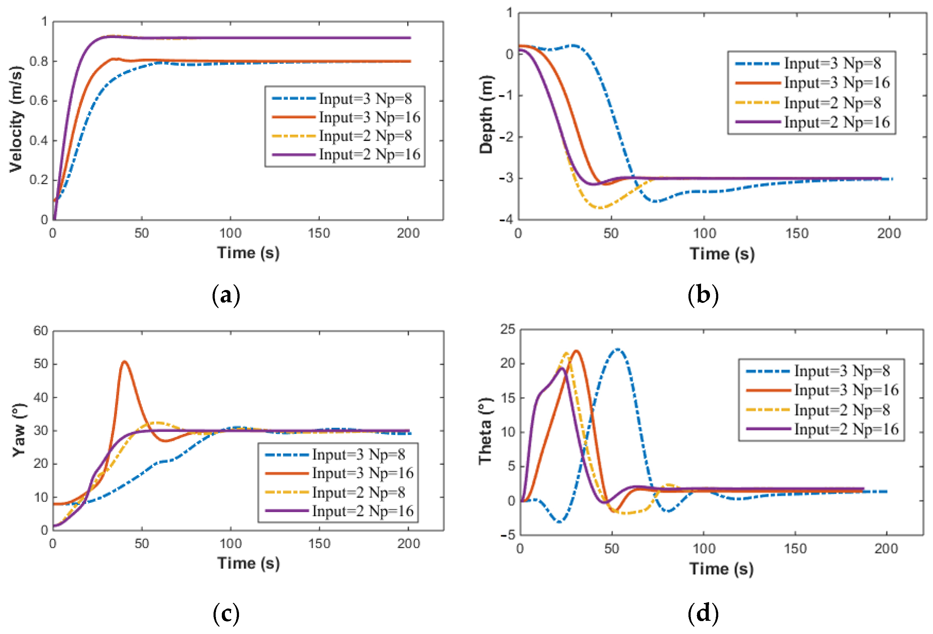
is also set to 8 and 16 for these simulations. The simulation results are presented in
Figure 16 and
Figure 17.
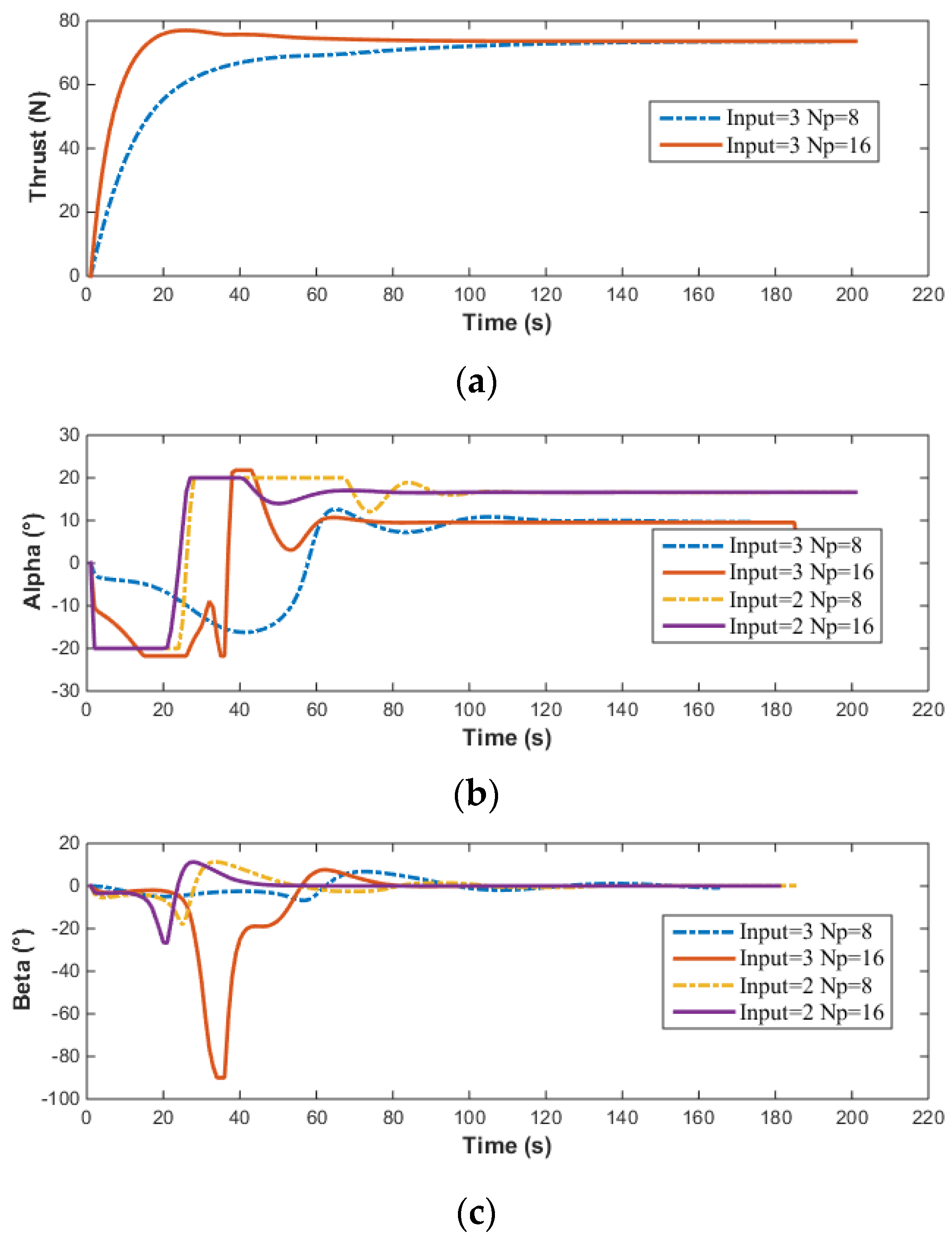
At this point, the input to the vector thruster is:
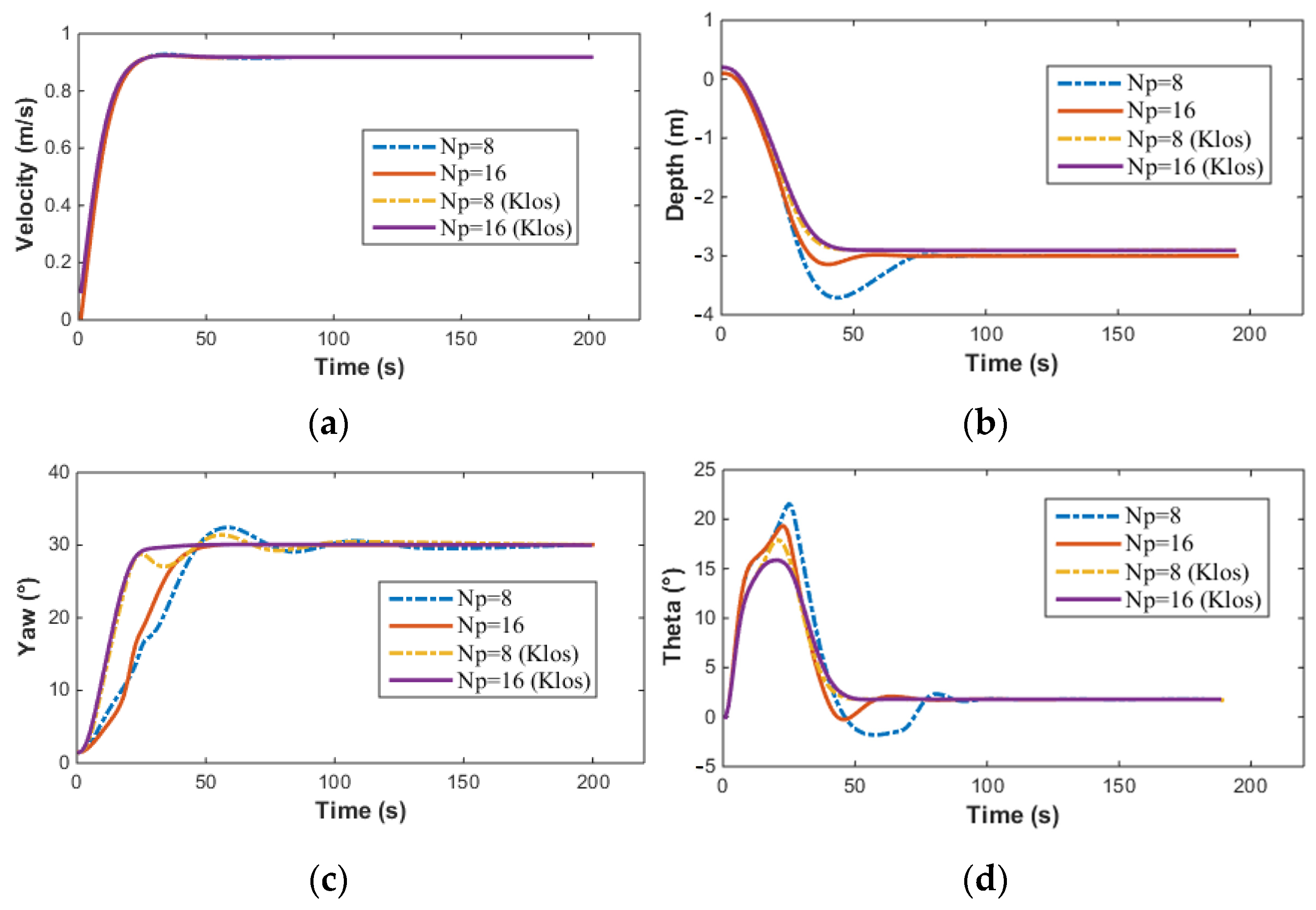
The above simulation results compare the effects of the prediction horizon and the number of control inputs on the simulation results. The smaller the prediction horizon, the lower the required computing power. A shorter prediction horizon requires less computational power. However, the control precision when is significantly higher than when . As the prediction horizon increases, the overshoot decreases, the adjustment time shortens, and the control precision improves. Additionally, it can be observed that the control input becomes smoother as the prediction horizon increases.
From
Figure 17, it can also be noted that when no velocity control is applied to the AUV, the velocity converges to
. However, when velocity control is implemented, the AUV converges to the target velocity
. It is evident from the graphs that under the same prediction horizon
, implementing velocity control does not change the control precision of the heading angle, the pitch angle, or the depth, but their adjustment times increase significantly. Furthermore, the time taken by the MPC solver also increases when velocity control is applied. The corresponding computation times for the three cost functions mentioned are presented in
Table 5 below.
After considering both computational power and control precision, the prediction horizon
is determined to be 16, and no velocity control is applied. It is also important to note that the depth control of underactuated AUVs is typically not achieved by directly controlling the depth but rather indirectly through the control of the pitch angle. When employing the Line-Of-Sight (LOS) method, the target pitch angle is given by:
In the above equation,
represents the look-ahead distance, which is typically determined based on the motion characteristics of the AUV. In this paper, for the experiments and simulations, the target depth is set to
. Moreover, due to the AUV’s negative-lift shape, its motion in the vertical plane is inherently unstable, and the control input from the vector thruster is limited. In practical control, it is necessary to constrain the pitch angle variation range of the AUV. By setting
and substituting it into the equation above, we can calculate the maximum range of pitch angle variation for the AUV during its descent from the water surface to the target depth as:
During the simulation, the error state cost function is set to
with a weight coefficient
,
,
, and the parameters
m,
are defined. The prediction horizon
is set to both 8 and 16, and the simulation results are compared against those obtained with an
error state cost function. The results are presented in
Figure 18 and
Figure 19 as shown.
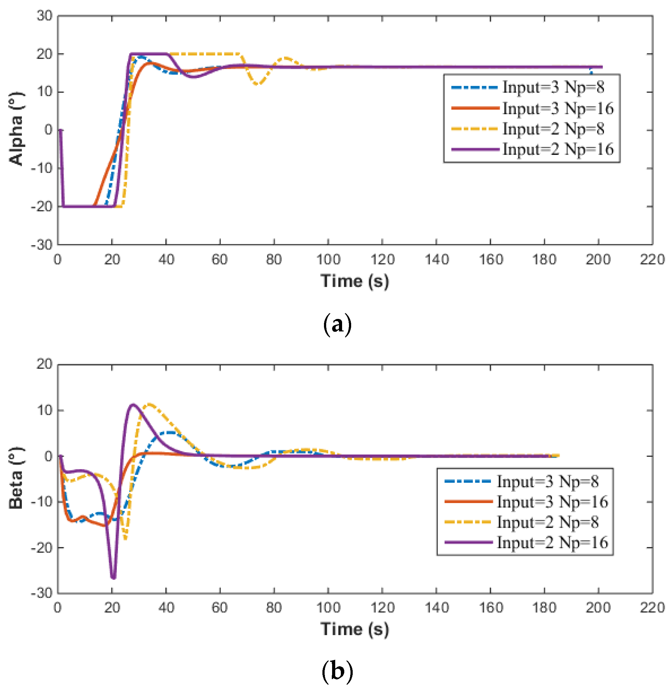
At this point, the input to the vector thruster is:
In
Figure 18,
and
represents the results of depth control based on the LOS method. Since no velocity control is implemented, the velocity response curves for both methods are identical. For depth control, due to the limitation on the pitch angle, when using the LOS method, the maximum pitch angle of the AUV is
, and there is no overshoot in the depth control. The simulation results demonstrate that the LOS-based depth control method achieves better performance. The object of this study is the AUV with vector propulsion. According to Equation (1), the control inputs
,
, and
of the AUV are mutually coupled. When controlling three variables simultaneously (speed, heading, depth), the NMPC controller must resolve coupled dynamics and trade-offs between conflicting objectives (e.g., AUV uses a vector thruster, and speed adjustment will inevitably disrupt depth stability). This higher-dimensional optimization problem introduces stronger nonlinear interactions, making convergence more sensitive to the prediction horizon (
Np). In contrast, the two-input case (fixed speed) simplifies the problem by decoupling speed dynamics, thereby reducing computational complexity and improving solution consistency. Multi-variable NMPC with a long horizon is more sensitive to the initial guess of the optimization. As shown in
Figure 19, in the case of three-input, a suboptimal initial guess leads to a longer convergence time and may cause the solution to diverge, whereas the two-input scenario benefits from simpler dynamics and more stable convergence.
Through simulation analysis, the MPC utilizing the LOS method was identified as the control scheme for the AUV. As disturbances were not considered in the simulation, to validate the effectiveness of the MPC control scheme under conditions free from external interferences and ensure consistency between the simulation and actual test environment, tests were conducted in a still water tank environment without any disturbance. The objective of the tests was to indirectly judge whether the accuracy of the AUV’s hydrodynamic coefficient calculations met the actual engineering application requirements by evaluating its control precision. The following
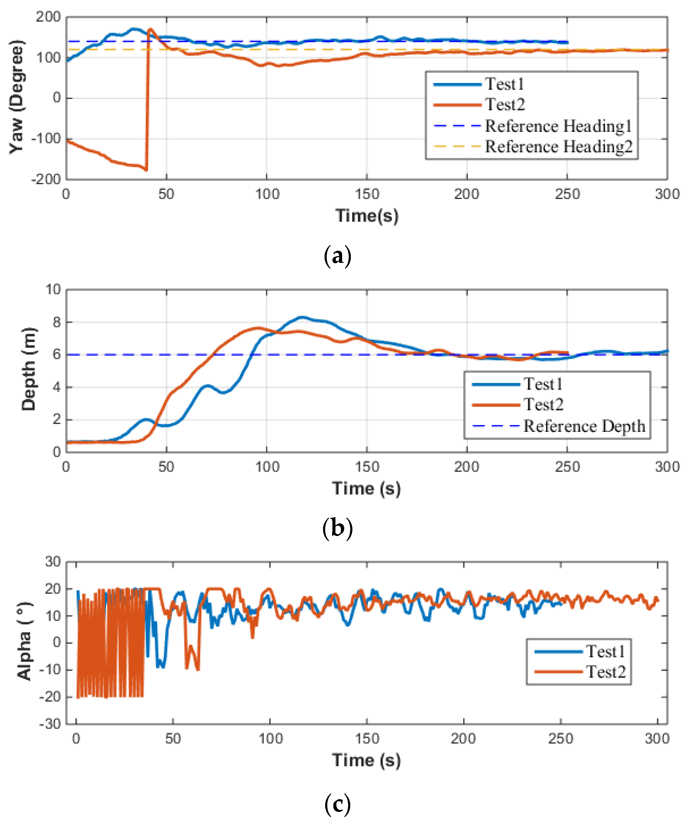
Figure 20 demonstrates the consistency between the control parameters used in the LOS-based depth control method for the AUV and those set during simulation, showcasing the results obtained from multiple tests conducted in the water tank environment.
It can be observed from
Figure 20 that while the speed of the AUV was not specifically controlled, the three test results exhibited good repeatability. In terms of depth control, the AUV showed minimal overshoot, and the depth in all three tests converged to the target depth. For heading angle control, given that the pool is oriented north-south, when the AUV moves linearly in this direction, its natural heading angle is 0°. Consequently, when setting up the heading control experiment, the target heading angle is set to 0°, and the heading control capability is evaluated by assigning various initial heading angles to the AUV. The experimental results indicated that even with varying initial heading angles, the AUV’s heading angle control maintained high precision, successfully adjusting and maintaining the heading angle near 0°. The largest difference between simulation and testing lies in the control of the pitch angle. Overall, the pitch angle varies within a limited range of approximately
. The sources of error here are similar to those in open-loop testing. In practical engineering applications of AUVs, where accurate hydrodynamic coefficients may not be readily available, it is necessary to consider the impact of errors and design MPC controllers with higher robustness. Furthermore, the actual input to the AUV’s vector thruster is illustrated in
Figure 21 below.
Figure 22 shows that the actuator of the vector thruster undergoes a relatively slow change process, which satisfies the physical constraints of the vector thruster.
Prior to conducting MPC control tests, extensive open-loop tests in the pool and model-free PID control tests offshore were performed on this AUV.
Figure 22 describes the design approach and relevant test results of a PID controller designed specifically for the AUV’s vector thruster. Comparing the control effects of MPC and PID, PID control is prone to overshooting, while MPC exhibits no overshooting phenomenon. When contrasting the vector thruster outputs,
and
(i.e., the inputs to the AUV), obtained through MPC and PID, respectively, it becomes evident that when a PID-based control strategy is adopted, the AUV’s motion control system, inherently a complex multi-input multi-output system, experiences significant coupling effects among its various thrust inputs. This coupling results in more drastic variations in the vector thruster outputs (
and
) after decoupling via PID control, thereby increasing the actuator’s operating frequency and ultimately leading to a substantial increase in control energy consumption. More crucially, the current control system fails to adequately consider the physical performance constraints of the vector thruster, such as output frequency limitations, which prevent the actual output values from matching the high-frequency outputs decoupled by PID control. This causes control delays and may even lead to degraded control performance or complete loss of control. Additionally, during actual offshore testing, the vector thruster’s frequent high-frequency outputs exacerbate the risk of mechanical failures or actuator damage, further complicating maintenance efforts. In contrast, the vector thruster outputs obtained through MPC exhibit smoother variations, effectively eliminating the drawbacks associated with PID control.


 ,
, 


