Article

Establishment and Evaluation of an Ensemble Bias Correction Framework for the Short-Term Numerical Forecasting on Lower Atmospheric Ducts

1
State Key Laboratory of Physical Oceanography, Qingdao 266001, China
2
Institute of Oceanographic Instrumentation, Qilu University of Technology (Shandong Academy of Sciences), Qingdao 266001, China
3
College of Meteorology and Oceanography, National University of Defense Technology, Changsha 410003, China
4
College of Information Science and Technology, Qingdao University of Science and Technology, Qingdao 260061, China
5
Department of Computer Science, University of Exeter, Exeter EX4 4RN, UK
6
Shandong Provincial Key Laboratory of Marine Engineering Geology and the Environment, Ocean University of China, Qingdao 266100, China
*
Author to whom correspondence should be addressed.
J. Mar. Sci. Eng. 2025, 13(12), 2397; https://doi.org/10.3390/jmse13122397
Submission received: 18 November 2025 / Revised: 10 December 2025 / Accepted: 13 December 2025 / Published: 17 December 2025
(This article belongs to the Special Issue Artificial Intelligence and Its Application in Ocean Engineering)

Abstract

Based on the COAWST (Coupled Ocean–Atmosphere–Wave–Sediment Transport) model, this study developed an atmospheric refractivity forecasting model incorporating ensemble bias correction by combining five bias correction algorithms with the Bayesian Model Averaging (BMA) method. Hindcast tests conducted over the Yellow Sea and Bohai Sea regions demonstrated that the ensemble bias correction enhanced both forecasting accuracy and adaptability. On the one hand, the corrected forecasting outperformed the original COAWST model in terms of mean error (ME), root mean square error (RMSE), and correlation coefficient (CC), with the RMSE reduced by approximately 20% below 3000 m altitude. On the other hand, the corrected forecasting reduced the uncertainty associated with the performance of different algorithms. In particular, during typhoon events, the corrected forecasting maintained stable bias characteristics across different height layers through dynamic weight adjustment. Throughout the hindcast period, the ME of the corrected forecasting was lower than that of any single bias correction algorithm. Moreover, compared with other ensemble methods, the corrected forecasting developed in this study achieved more flexible weight allocation through Bayesian optimization, resulting in lower ME. In addition, the corrected forecasting maintained an improvement of approximately 28% in bias reduction even at a 72 h forecasting lead time, demonstrating their robustness and reliability under complex weather conditions.

1. Introduction

Atmospheric refractivity characterizes the degree of refraction that occurs when electromagnetic waves propagate through the atmosphere. Atmospheric refractivity affects remote sensing image positioning, electromagnetic wave propagation, and the performance of air–ground data links and communication systems [1,2]. For electromagnetic waves in the frequency range of 100 MHz to 100 GHz, S. Babin et al. established and refined an empirical model of atmospheric refractivity, expressing it as a function of meteorological parameters such as air temperature, air pressure, water vapor pressure, and altitude [3]. After considering the effect of Earth’s curvature on ground-level electromagnetic wave propagation, atmospheric refractivity can be converted to modified atmospheric refractivity [4]. The formula is
M = N + 0.157 × H
where
N = 77.6 T ( p + 4810 e T )
Here, M represents the modified atmospheric refractivity (M−units), N represents the refractivity (N−units), H represents the altitude (m), T represents air temperature (K), P represents air pressure (hPa), and e denotes water vapor pressure, which can be calculated using the following equation:
e = q P ε + 1 ε q
where q denotes the specific humidity (g/kg), and ε is a constant equal to 0.622.
Accurate forecasting of the modified atmospheric refractivity profile is the data foundation for identifying atmospheric duct phenomena [5]. An atmospheric duct refers to a special stratification of the atmosphere that enables radio waves in the very high frequency and microwave bands to achieve over-ranged propagation [6,7]. Generally, the atmospheric duct phenomenon is considered to occur when the vertical gradient of the modified atmospheric refractivity falls below a certain threshold value [5].
The presence of an atmospheric duct alters the range and path of electromagnetic wave propagation, demonstrating strong application value in fields such as shortwave communication and radar detection, while also introducing interference to normal operations. For example, an atmospheric duct can enable radar electromagnetic waves to propagate over several times greater distances with very low transmission loss, but simultaneously create a detection blind zone above the duct layer, where target activities cannot be perceived by radar [8].
To accurately forecast the modified atmospheric refractivity or atmospheric duct phenomena, two main approaches have traditionally been employed: numerical forecasting and empirical methods. Numerical forecasting utilizes numerical weather prediction models to conduct routine weather forecasting and subsequently diagnose various atmospheric phenomena based on the forecasting results. Empirical methods employ mathematical or regression methods to establish statistical models that estimate future changes in historical data. This purely data-driven approach is typically used for nowcasting within a 3 h time window; its forecasting accuracy may decrease rapidly as the forecasting lead time increases [9,10].
With the continuous development of Artificial Intelligence (AI) algorithms, many researchers have attempted to combine numerical forecasting models with AI algorithms using various approaches, aiming to improve the physical interpretability of AI algorithms while further enhancing the accuracy of weather forecasting. For example, Berry et al. proposed a nonparametric Bayesian method based on the Reproducing Kernel Hilbert Space (RKHS) that can be integrated with any data assimilation system, including the Ensemble Kalman Filter (EnKF), to correct observational biases. Simulation results demonstrated that this method reduced the mean relative root mean square error (RMSE) by more than 40% for several key variables, such as high, middle, and low cloud fractions, compared with the standard EnKF [11]. Rasp et al. employed deep neural networks to learn sub-grid physical processes in the Super Parameterized Community Atmosphere Model (SPCAM) and successfully embedded it into a global climate model to replace traditional cloud and radiation parameterization schemes. The results showed that the neural network version of Community Atmosphere Model, NNCAM, achieved approximately 20 times faster computational speed than the original model [12].
Among the various studies that combine numerical forecasting models with AI techniques, AI-based bias correction has proven to be one of the most effective approaches for rapidly improving numerical forecasting accuracy. For example, Han et al. proposed a CU-net deep learning method to correct the gridded bias in wind speed forecasting from the European Centre for Medium-Range Weather Forecast (ECMWF) Integrated Forecasting System (IFS) model over North China, finding that compared with the conventional Anomaly Numerical-correction with Observations (ANO) method, the CU-net improved forecasting accuracy by 18.57% for the next 24 h and by 3.70% for the next 240 h [13]. Yao et al. combined the Weather Research and Forecasting (WRF) model with a Bidirectional Long Short-Term Memory (Bi-LSTM) network to correct biases in hourly precipitation forecasting products over Anhui Province in eastern China. Their results showed that the RMSE decreased from 1.91 mm/h to 1.08 mm/h after correction [14]. Wei et al. proposed and applied an improved Trajectory Gated Recurrent Unit (TrajGRU) model for real-time bias correction of significant wave height gridded forecasting from the ECMWF global model. The corrected results reduced the mean absolute error (MAE) by 12.97%~46.24% in spring and by 13.79%~38.95% in winter [15].
However, researchers found in practical applications that bias correction results obtained from a single algorithm often exhibited substantial uncertainty. In other words, no single algorithm was able to guarantee high correction accuracy under all circumstances [16,17].
To reduce the uncertainty associated with one single algorithm, ensemble averaging is considered one of the most effective approaches. The ensemble method combines the forecasting results of multiple models, fully leveraging the advantage of each model to significantly improve forecasting accuracy [18]. While recent studies have demonstrated that ensemble learning outperforms single deterministic models in forecasting temperature and wind speed [19], current ensemble approaches for bias correction still face critical limitations. Most existing ensemble methods rely on simple arithmetic averaging or assign static, fixed weights to member models based on historical performance. This static approach assumes that the contribution of each model remains constant throughout the forecasting period. In reality, the performance of single algorithms varies significantly under different weather regimes, especially during rapidly changing or extreme conditions. These limitations highlight the need for a dynamic weighting strategy.
The Bayesian Model Averaging (BMA) algorithm is one of the classical multi-model ensemble forecasting approaches. In the field of hydrometeorological forecasting, the BMA method has been proven to deliver outstanding forecasting performance [20,21]. For example, Duan et al. applied the BMA method to integrate the forecasting results from nine different hydrological models. The results showed that compared with the best single model, the BMA-based ensemble reduced the RMSE by 10.79% and the MAE by 4.60% [22]. Li et al. proposed an effective framework by combining the BMA method with three deep learning models for short-term water level forecasting at five stations in Poyang Lake. The results demonstrated that compared with single deep learning models, the BMA-based ensemble significantly improved forecasting accuracy in different forecasting lead times, reducing the relative error (RE) by 8.89% for 1-day forecasting and by 41.24% for 3-day forecasting ahead [23].
In the past, many researchers established various numerical forecasting models for atmospheric refractivity and atmospheric duct. Our earlier work also established an atmospheric duct forecasting model based on the Coupled Ocean–Atmosphere–Wave–Sediment Transport (COAWST) system. The 72 h forecasting tests over the South China Sea indicated that, compared with radiosonde observation data within the region, the 24 h forecast of modified atmospheric refractivity (calculated using Equations (1)–(3)) by the duct forecasting model had a mean error (ME) of 7.10 M, which is lower than the 12.90 M error of the ERA5 (ECMWF Reanalysis v5) data. However, several critical issues were identified. The RMSE of modified atmospheric refractivity forecasts was particularly high (>10 M) below 1000 m altitude, precisely where atmospheric duct conditions most frequently occurred. This indicated systematic deficiencies in representing atmospheric boundary layer processes within the COAWST model [24]. Specifically, during extreme-weather scenarios such as typhoons, although COAWST outperformed the single weather WRF model by coupling oceanic and wave components, its core atmospheric physical parameterizations still struggled to resolve the complex boundary layer structures required for accurate refractivity profiling, leading to persistent bias in wind, humidity, and wave interactions [25].
To address these deficiencies, there were generally three pathways: (1) improving the model’s internal physical schemes to reduce primitive systematic errors; (2) employing advanced data assimilation to constrain initial conditions; or (3) implementing post-processing based on model outputs. While the first two approaches required substantial computational resources and deep modifications to the model kernel, post-processing offered a more direct and computationally efficient alternative for operational forecasting. Therefore, this study adopted the third approach. By applying multiple bias-correction algorithms and integrating them through a multi-model ensemble framework, the approach aimed to not only correct systematic bias but also mitigate the uncertainty associated with any single correction method.
Based on the identified limitations of the COAWST model, single correction method and static ensemble methods, this study proposes a comprehensive forecasting framework. A diverse set of bias-correction algorithms is introduced—including the Convolutional Neural Network (CNN), Long Short-Term Memory (LSTM), Gated Recurrent Unit (GRU), Backpropagation Neural Network (BP), and Model Output Statistics (MOS), as well as the BMA-based ensemble method. By performing multi-model ensemble correction of forecasting biases, a new atmospheric refractivity forecasting framework will be established as follows. Using this system, a series of simulation tests will be designed to evaluate their forecasting accuracy and to investigate the role of the multi-model ensemble method in improving forecasting bias correction performance.

2. Model, Algorithms and Data

2.1. COAWST Model

The COAWST model, developed by Warner et al., is an ocean–atmosphere coupled modeling system. It integrates several component models, including the WRF, the Regional Ocean Modeling System (ROMS), and Simulating Waves Nearshore (SWAN). The Model Coupling Toolkit (MCT) orchestrates the computations of each component model, and facilitates variable transfer and exchange among the component models through parallel coupling [26].

2.2. Bias Correction Algorithms

2.2.1. Backpropagation Neural Network (BPNN)

The BPNN, proposed by Rumelhart and McClelland in 1986, has been widely applied in fields such as pattern recognition and forecasting [27,28,29]. This model employs a bias backpropagation mechanism, using the gradient descent algorithm to iteratively adjust the network weights in order to minimize output bias and optimize forecasting performance [30].

2.2.2. Convolutional Neural Network (CNN)

The CNN is a type of feedforward neural network inspired by the visual cortex, capable of automatically extracting features through convolutional kernels [31]. In this study, the one-dimensional convolutional neural network (1-D CNN) was employed to handle time series data. By adjusting the kernel size and stride, the 1-D CNN was able to efficiently capture local features within the sequence while maintaining a balance between modeling capability and computational efficiency [32].

2.2.3. Gated Recurrent Unit (GRU)

The GRU is a simplified variant of the recurrent neural network (RNN), similar to the LSTM network, and is designed to capture long-term dependencies in time series data [33]. The GRU regulates information flow through update and reset gates, featuring a simpler architecture, fewer parameters, and more efficient training compared with LSTM. It can also effectively mitigate the vanishing gradient problem [34].

2.2.4. Long Short-Term Memory (LSTM)

The LSTM network, proposed by Hochreiter and Schmidhuber, is designed to alleviate the long-term dependency and vanishing gradient problems inherent in traditional recurrent neural networks [35,36]. Its architecture consists of memory cells, input gates, output gates, and forget gates, which together form a gating mechanism that enables selective retention, updating, and output of critical information.

2.2.5. Model Output Statistics (MOS)

MOS is an objective forecasting technique based on statistical methods that aims to establish a quantitative relationship between the numerical forecasting outputs and the observations [37]. The core approach of MOS is polynomial fitting.

2.3. Bayesian Model Averaging Algorithm

BMA is a statistical method used to integrate the forecasting outputs of multiple models, thereby producing more reliable and sophisticated forecasting [38].
The fundamental principle of BMA can be described as follows. Let y represent the variable to be forecast, and let the model space f = f 1 , f 2 , , f K represent the set of all bias-correction model forecasts, where K represents the number of models, and D = y 1 , y 2 , , y T represents the observations of length T. According to the law of total probability, the BMA Probability Density Function (PDF) of y can be expressed as
p ( y | D ) = k = 1 K p ( f k | D ) · p k ( y | f k , D )
Here, under the given model k, p k ( y | f k , D ) represents the conditional PDF of the forecasting variable y, and p ( f k | D ) represents the posterior probability of the k th model; it reflects the degree of agreement between each ensemble member and the observations during the training process. To ensure comparability among all ensemble members, the model weights were constrained as w k = p ( f k | D ) and k = 1 K w k = 1 . The posterior probability for any element f j in the model space, given dataset D, can be expressed as
p ( f j | D ) = p ( f j ) p ( D | f j ) k = 1 K p ( f k ) p ( D | f k ) .
The marginal or integrated likelihood of each model, p ( D | f j ) , can be expressed as
p ( D | f j ) = F ( D | θ j , f j ) P ( θ j | f j ) d θ j ,
where θ j is the parameter vector of model f j that needs to be estimated from the observed data D. F ( D | θ j , f j ) is the likelihood function representing the probability of observing data D given parameters θ j and model f j , and P ( θ j | f j ) is the prior distribution reflecting our initial beliefs about the parameters before observing the data. The marginal likelihood integrates over all possible parameter values, weighting each likelihood by its prior probability. Accordingly, the posterior mean and variance of the BMA forecasting can be expressed as [39]
E [ y | D ] = k = 1 K p ( f k | D ) · E [ p k ( y | f k , D ) ] = k = 1 K w k μ k ,
V a r [ y | D ] = k = 1 K w k ( μ k i = 1 K w i μ i ) 2 + k = 1 K w k   σ k 2   ,
Here, σ k 2   represents the variance between the model forecasting f k and the observations D. μ k represents the expected value of the y under model f k given the observed data D. BMA forecasting is the weighted average of the single model forecasting, as shown in Equation (7), while the BMA variance serves as a quantitative measure of the forecasting uncertainty. As illustrated in Equation (8), it consists of both the between-model variance and the within-model variance, corresponding to the first and second terms on the right-hand side, respectively. These two characteristics make the BMA method widely applicable in meteorological and hydrological forecasting.
In this study, the conditional probability distribution p k ( y | f k , D ) was assumed to follow a Gaussian distribution [40]. However, since the probability distribution of the modified atmospheric refractivity typically exhibited non-Gaussian characteristics, it was necessary to perform data preprocessing to enhance its approximation to a Gaussian form. To estimate the weights and variances of the BMA method, the Markov Chain Monte Carlo (MCMC) method was employed [41]. In the Bayesian framework, the observed data D is used to update prior beliefs about the parameters θ j through Bayes’ theorem, yielding posterior distributions. MCMC constructs a Markov chain whose stationary distribution corresponds to the posterior distribution of the model parameters, from which a large number of posterior samples were drawn to numerically estimate the marginal likelihood p ( D | f j ) for each model. Subsequently, Bayes’ theorem was used to compute the posterior model probability p ( f j | D ) , thereby deriving the BMA model weights. This approach effectively approximates complex posterior distributions in the absence of analytical solutions, improving the stability and accuracy of weight estimation. Detailed theoretical and methodological descriptions of MCMC can be found in the work of Gong et al. [42].
To prevent excessive dispersion in weight allocation, this study introduced a threshold-based decision mechanism during the dynamic updating stage. When significant differences existed among model weights, if the correction result of a particular algorithm deviated from the observations by less than 0.1, the system identified this algorithm as the optimal model for the current period and assigned it a weight of 1, while correspondingly reducing the weights of other models. This adaptive strategy helped the system dynamically recognize the dominant model under different weather conditions, thereby enhancing the robustness and reliability of the ensemble forecasting.
In this study, the ensemble members consisted of forecasting corrected by five algorithms: LSTM, CNN, GRU, BPNN, and MOS. Prior to performing the ensemble averaging, both the forecasting and observations were transformed using the Box–Cox method [43] to approximate a Gaussian distribution. Subsequently, Bayesian inference for the ensemble members was conducted using the Markov Chain Monte Carlo (MCMC) method. By sampling extensively from the posterior distributions of the model parameters, the marginal likelihood of each ensemble member was estimated. Based on these estimates, the posterior probabilities (i.e., BMA weights) were derived using Bayes’ theorem. The final deterministic BMA forecast was then obtained by weighting the predictions of all ensemble members according to these posterior probabilities. Furthermore, using the intra-model and inter-model variances derived from MCMC sampling, a complete BMA predictive distribution was constructed, from which the 90% confidence interval of the probabilistic forecast was computed.

2.4. Framework for Lower Atmospheric Ducts’ Forecasting

The driving data for each sub-model were obtained as follows. The WRF sub-model was driven by the Global Forecast System (GFS; data source: https://www.ncei.noaa.gov/products/, accessed on 12 December 2025), while its data assimilation module was driven by the Global Data Assimilation System (GDAS; data source: https://www.ncei.noaa.gov/data/ncep-global-data-assimilation/access/, accessed on 12 December 2025). The ROMS sub-model was driven by the Global Ocean Forecasting System (GOFS, available online at https://www.hycom.org/dataserver/, accessed on 12 December 2025) of the Hybrid Coordinate Oceanic Circulation Model (HYCOM) model. The SWAN sub-model was driven by the GFS_wave dataset.
Figure 1 shows the operational flowchart of the forecasting framework. First, atmospheric forcing data and assimilation initial fields were downloaded from the data servers. After undergoing quality control, interpolation, and format conversion, these datasets were processed into a unified initial forcing field. Based on these processed forcing and assimilation datasets, model preprocessing was then conducted. Specifically, GFS forcing data were converted through the WPS (WRF Preprocessing System) to generate the atmospheric initial and boundary conditions required by the WRF model, while GDAS assimilation data were incorporated into the WRF initial and boundary files through the three-dimensional variational assimilation module (WRF-3DVar). Meanwhile, the GOFS and wave data were processed through the ROMS and SWAN preprocessing modules to produce the initial and boundary conditions for the ocean and wave models, respectively. Subsequently, the COAWST model read all atmospheric, oceanic, and wave boundary conditions, together with static fields, and performed time integration to generate 72 h forecasts. From the model outputs, key atmospheric variables—such as air pressure, humidity, and air temperature—were extracted, and the modified atmospheric refractivity was computed using Equations (1)–(3), forming the initial forecasts. The forecasts were then corrected using five bias-correction algorithms—MOS, BPNN, LSTM, GRU, and CNN—to obtain the bias-corrected refractivity forecasts. Finally, based on the BMA method, model weights were estimated from all correction algorithms and the historical observations. The corrected outputs from the five models were then combined through weighted averaging to produce the final optimal ensemble forecasting of the modified atmospheric refractivity.

2.5. Data Description

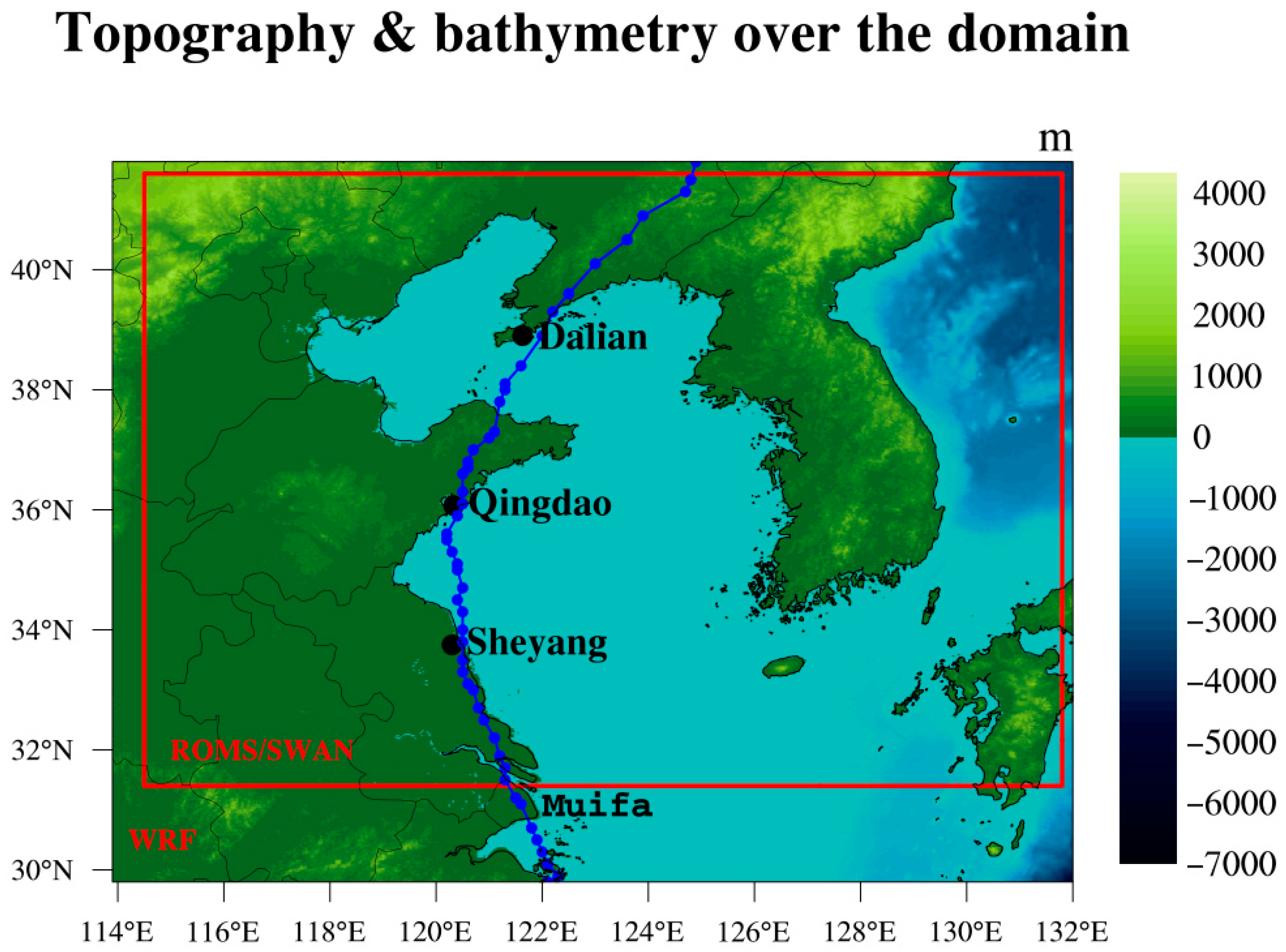
In this study, radiosonde observation data from the Yellow Sea and Bohai Sea regions were primarily used for model training and validation. These data were obtained from the University of Wyoming radiosonde observation data website (http://weather.uwyo.edu/, accessed on 12 December 2025), and the selected radiosonde stations include Dalian, Qingdao, and Sheyang, whose geographic locations are marked by black dots in Figure 2. The radiosonde observation data included key atmospheric variables such as air pressure, altitude, air temperature, dew point temperature, relative humidity, and water vapor mixing ratio, with an observation frequency of twice daily (00 h UTC and 12 h UTC).
During the validation process, the radiosonde observation data were used as the benchmark reference, while the ERA5 reanalysis data (available at https://www.ecmwf.int/en/forecasts/dataset/ecmwf-reanalysis-v5, accessed on 12 December 2025) from ECMWF was also employed as a reference. The ERA5 data combines global climate model with ground-based and satellite observations, offering high spatiotemporal resolution. Its horizontal resolution is 0.25° × 0.25°, with 37 vertical pressure levels ranging from 1000 hPa to 1 hPa and a temporal resolution of 1 h.

3. Experimental Design

3.1. Model Configuration

The domain in this study included the Yellow Sea, Bohai Sea, and adjacent marine areas, as shown in Figure 2. The configuration of the COAWST (developed by the U.S. Geological Survey, Woods Hole, MA, USA)model’s parameterization schemes is listed as follows: the WRF module (developed by the National Center for Atmospheric Research, Boulder, CO, USA) employed grids of 310 × 240 with a horizontal resolution of 6 km and 39 vertical levels; the ROMS and SWAN modules used grids of 300 × 220 with the same horizontal resolution as WRF, and ROMS includes 16 vertical layers in the vertical direction. In the WRF model, the selected physical parameterization schemes included the WSM6 (WRF Single-Moment 6-Class) cloud microphysics scheme, MM5 (the fifth-Generation Penn State/NCAR Mesoscale Model) similarity scheme (surface layer), RRTM (Rapid Radiative Transfer Model) longwave radiation, Dudhia shortwave radiation, Noah Land Surface Model (Noah-LSM), and the GF (Grell–Freitas) cumulus convection parameterization scheme. In the ROMS configuration, vertical turbulent mixing was represented by the Mellor–Yamada turbulence closure scheme, and the Flather boundary condition was applied to enable the free propagation of wind-driven currents and tidal signals, allowing the model to reproduce anisotropic ocean current characteristics.

3.2. Training Settings and Neural Network Architectures

The bias correction models in this study utilized only the time series of the COAWST-simulated modified atmospheric refractivity and the corresponding historical observations as input features, excluding temperature, humidity, air pressure or other factors. Although atmospheric ducts were physically driven by these meteorological variables, this univariate input strategy was adopted based on two key considerations. First, the primary objective of this study was to investigate the performance differences among various correction algorithms and to evaluate the effectiveness of the ensemble framework itself. Incorporating multivariate inputs would have introduced additional complexity, making it difficult to determine whether performance gains stemmed from the algorithm structure or from the supplemental input information. Second, the performance of multivariate models typically depended on specific variable combinations. When the correction target changed, this strategy required re-screening input variables, thereby limiting its generalizability. In contrast, the approach adopted here—relying solely on the target variable’s own bias change—provided a generic, end-to-end solution that could be applied to other meteorological parameters without extensive re-optimization.
Input data were processed using a sliding-window strategy with a window length of 12 h. The mean squared error (MSE) was used as the loss function, and model training was optimized with the Adam algorithm [44]. To prevent overfitting, early stopping [45] was applied with a patience of three epochs; training was terminated once the validation loss failed to decrease for three consecutive epochs, and the model parameters were rolled back to the state with the minimum validation loss. All inputs were standardized prior to training (zero-mean and unit-variance).
To ensure the reproducibility of the proposed forecasting framework, the architectures and hyperparameters of all neural network models—BPNN, CNN, GRU, and LSTM—were explicitly defined. The BPNN model adopted a three-layer fully connected structure (10–50–78–1 nodes) with ReLU activation in the hidden layers and a batch size of 60. The CNN consisted of a single one-dimensional convolutional layer (2 input channels, 120 output channels, kernel size of 3, and padding of 1), followed by ReLU activation and flattening, with a batch size of 30. Both the GRU and LSTM models used two stacked recurrent layers with a hidden size of 60 and a batch size of 30. All models were implemented using the PyTorch version 3.12 framework.

3.3. Construction of Simulation Tests

The historical hindcast simulation for training covered the period from January 2016 to December 2021. The formal validation period was set 1–30 September 2022, totaling 30 days, during which continuous daily 72 h forecasting was performed. During the validation period, Typhoon Muifa passed northward through the study domain from 12:00 on 15 September to 12:00 on 16 September.
To evaluate the accuracy of the ensemble-corrected forecasting method developed in this study, several comparative tests were designed: the CTL test used the COAWST-forecasted modified atmospheric refractivity and atmospheric duct without any bias correction. The corrected forecasting tests by single algorithms were named as T1_BP, T1_MOS, T1_CNN, T1_GRU, and T1_LSTM, respectively. The T1_BMA test represented the ensemble bias-correction results obtained using the BMA method proposed in this study. Additionally, to further assess the performance of different ensemble approaches, two additional comparative tests were conducted; the T2_AM test applied an arithmetic average to combine the five bias-corrected forecasts. The T3_EM test employed a previously developed variable-weight ensemble averaging method, where the ensemble forecasting value M could be expressed as [46]
M e n s , d t = O d 1 ¯ + i = 1 N α i , d M i , d t M i , d 1 ¯ ,
Here, t Mens,dt denotes the ensemble forecasting for day d at time t; Od−1 represents the observations on the previous day d − 1; i is the forecasting member ID; and N is the total number of forecasting members, which in this case equals five; αi,d represents the weight of model Mi on day d, which can be calculated using the RMSE of Mi on day d − 1.
α i , d = E i , d 1 i = 1 N E i , d 1
Here, E is defined as the reciprocal of the RMSE computed over the 24 h of a day.

4. Results

4.1. Bias Statistics of the 24 h Forecasting Result for the Modified Atmospheric Refractivity

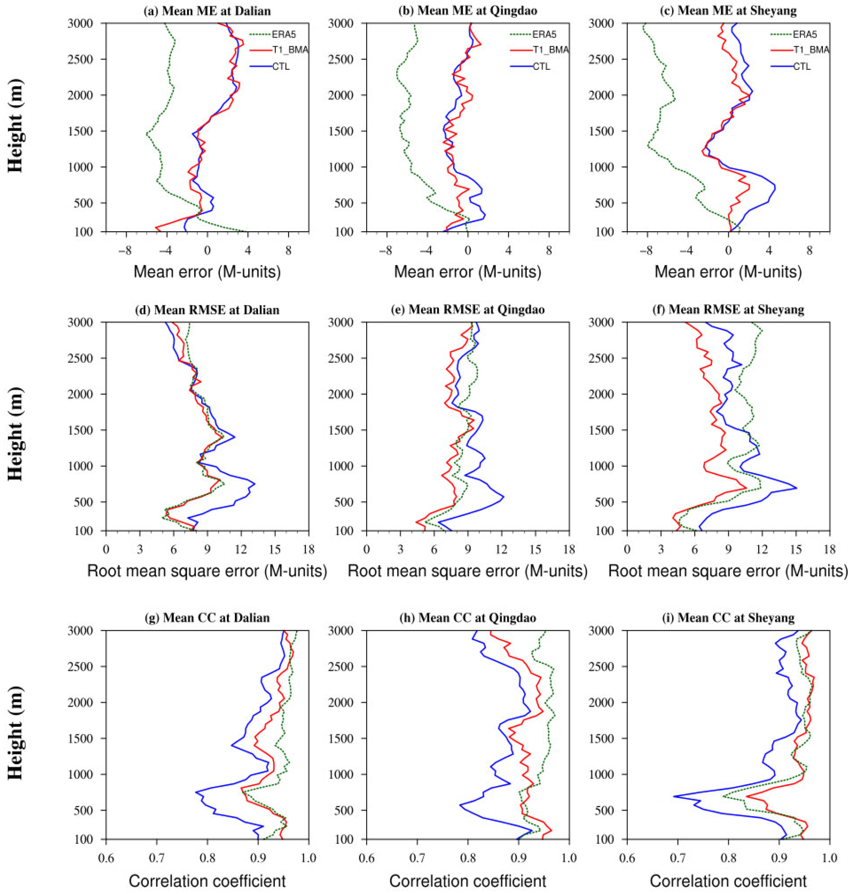
Figure 3 presents the vertical profiles of the 24 h forecasting indices at the Dalian, Qingdao, and Sheyang stations during September 2022, comparing three datasets: CTL, T1_BMA, and ERA5 reanalysis data. Specifically, Figure 3a–c show the ME profiles, with Figure 3d–f showing the RMSE profiles and Figure 3g–i showing the Correlation Coefficient (CC) vertical profiles.
From the shape of the vertical profiles, within the 3000 m altitude range, the RMSE of the model forecasting was relatively higher below 1000 m, and the overall bias gradually decreased with height. Due to the cancelation between positive and negative deviations, the ME exhibited relatively small variations across different altitudes. This indicated that the COAWST model’s performance within the atmospheric boundary layer still required improvement. Overall, the statistical indicators of the T1_BMA test at all three radiosonde stations were almost consistently superior to those of the CTL test, indicating a further enhancement in forecasting accuracy.
Specifically, the 24 h forecasting MEs of modified atmospheric refractivity in the T1_BMA test were 0.37 M, −0.83 M, and 0.05 M at the Dalian, Qingdao, and Sheyang stations, respectively. These MEs reduced by 42%, 28%, and 95% compared with those of the CTL test. As for RMSEs, the values of the T1_BMA test were 7.93 M, 7.63 M, and 7.21 M, respectively, corresponding to reductions of 10%, 18%, and 26% relative to the CTL test. The average CCs with the radiosonde observation data were 0.93, 0.91, and 0.94 for the three stations, which were 0.04, 0.05, and 0.05 higher than those of the CTL test, respectively. According to the study of Haack et al., the COAMPS (Coupled Ocean–Atmosphere Mesoscale Prediction System) and MetUM (Met Office’s Unified Model) models produced mean RMSE values of 11.10 M and 14.40 M, respectively, for modified atmospheric refractivity at an altitude of 112 m over Wallops Island, slightly higher than the simulation biases obtained in this study [47].
The MEs of the ERA5 data at the three stations were −3.50 M, −5.10 M, and −5.30 M, while its RMSE values were 8.12 M, 8.55 M, and 9.97 M, respectively, all of which were higher than those from the T1_BMA test. In terms of the CC with the observation data, the ERA5 data showed slightly higher values than the T1_BMA test, with values of 0.94, 0.94, and 0.92, respectively.
Figure 4 shows the Taylor diagrams of the 24 h forecasting of modified atmospheric refractivity from the CTL and T1_BMA tests, as well as the ERA5 data, at the Dalian, Qingdao, and Sheyang stations. The Taylor diagram includes both the CC and Standard Deviation (SD) dimensions. The intersection of unit arc 1 with the x-axis represents the reference point; the closer a series lies to this point, the better its overall statistical performance.
As shown in Figure 4a–c, after applying the BMA method for ensemble bias correction, the forecasting results at all three stations exhibited varying degrees of improvement, with the most pronounced enhancement observed at Sheyang Station. Compared with the CTL test, the CCs between the T1_BMA forecasting and the observation increased by 0.04, 0.05, and 0.06, respectively. It is worth noting that the SDs of the T1_BMA forecasting decreased relative to that of the CTL test, which was consistent with previous findings indicating that bias correction tended to reduce the variability of the forecast series to some extent. Although the SDs of the T1_BMA forecasting and ERA5 were generally lower than those of the original forecasting, this did not necessarily indicate a degradation in performance.

4.2. Comparison of Accuracy Differences Between the Ensemble Forecasting and Single Algorithm Members

To evaluate the effectiveness of the ensemble forecasting developed in this study, the 24 h forecasting biases of the T1_BMA test were compared with those of the five single correction algorithms (T1_BP, T1_CNN, T1_GRU, T1_LSTM, and T1_MOS).
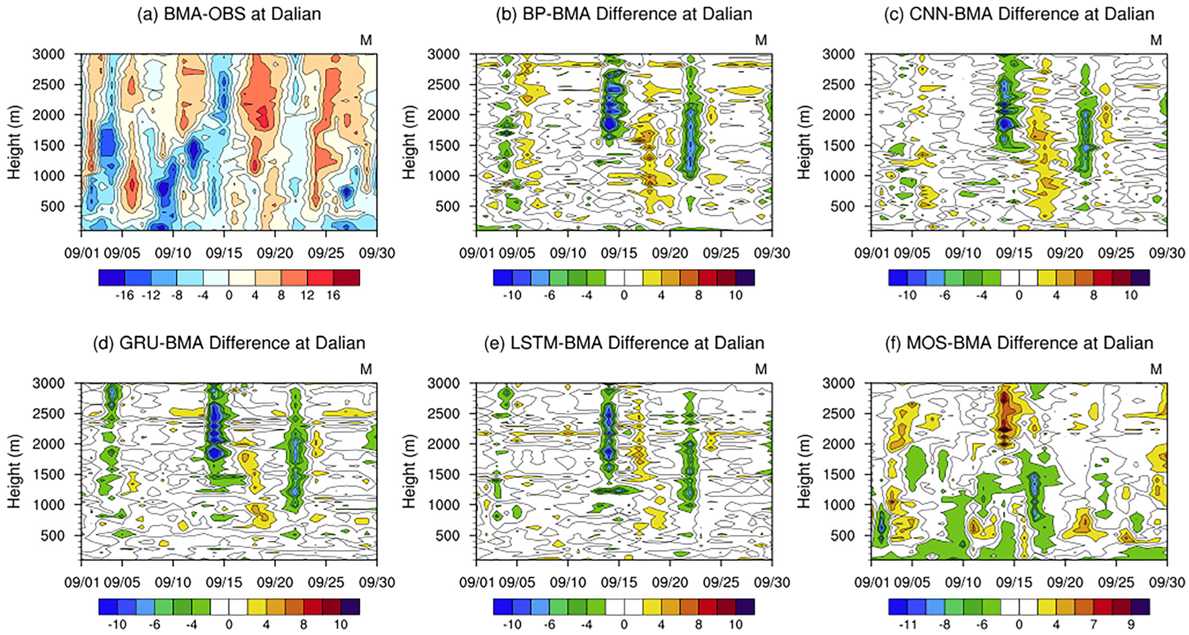
Figure 5 shows the two-dimensional time–height diagrams of forecasting biases at different altitudes over the Dalian station. Specifically, Figure 5a shows the temporal distribution of 24 h forecasting biases (T1_BMA − OBS) within the 3000 m altitude. For comparison, Figure 5b–f show the differences between each ensemble member and the T1_BMA forecasting (T1_BP − T1_BMA, T1_CNN − T1_BMA, T1_GRU − T1_BMA, T1_LSTM − T1_BMA, and T1_MOS − T1_BMA). By comparing the T1_BMA forecasting biases with the deviations of each ensemble member, the relative performance among the ensemble members can be examined horizontally.
As shown in Figure 5a, the forecasting biases in the T1_BMA test did not remain constant across all times and altitudes. The largest negative biases occurred around 10 September at altitudes between 500 m and 1500 m, with values approximately −20 M. Around September 21, when widespread convective weather developed in the study area, positive biases appeared at most altitudes. Interestingly, during the typhoon passage (15–16 September), the forecasting biases in the T1_BMA test did not increase significantly, indicating that the ensemble method enhanced the stability of forecasting accuracy during periods of rapid weather system evolution.
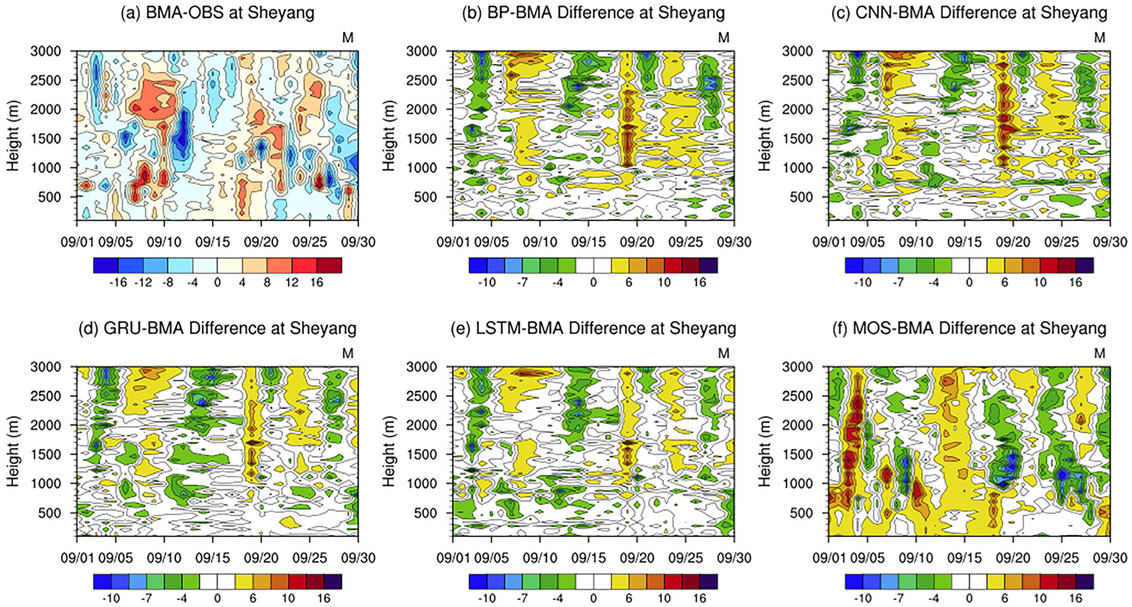
Figure 5b–f show the differences between each ensemble member and the T1_BMA test. When the color of the difference in a given period matches that in Figure 5a, it indicates that the member’s bias was higher than that of T1_BMA; conversely, when the color is opposite, it indicates a lower bias. During the simulation period, the spatial–temporal distributions of differences between the neural-network-based members and T1_BMA (Figure 5b–e) are largely consistent with the bias distribution in Figure 5a. This suggested that, in most cases, the forecasting biases of T1_BMA were smaller than those of T1_BP, T1_CNN, T1_GRU, and T1_LSTM. Around 15 September, a pronounced negative bias occurred between 1500 m and 3000 m for these members, indicating that all neural-network-based bias-correction algorithms performed poorly during that period.
As shown in Figure 5f, the polynomial-fitting-based MOS algorithm exhibited a larger bias difference compared with the other ensemble members, providing the T1_BMA test with greater flexibility in weight allocation to handle situations where multiple members produced similar biases. In Figure 5f, during the typhoon passage on 15–16 September, the T1_MOS test showed a positive bias between 2000 m and 3000 m and received a higher weight in the ensemble averaging process, which resulted in the T1_BMA test having smaller forecasting biases than the other four ensemble members during that period. However, this did not mean that the T1_MOS test consistently achieved the lowest biases at all altitudes. For example, on 10 September, the T1_MOS test exhibited a noticeable negative bias below 1500 m, while the other members showed little deviation from the ensemble averaging. Moreover, around 18–20 September, the forecasting biases of all members, including T1_MOS test, were largely consistent with one another, showing minimal differentiation, which led to a less effective ensemble averaging performance during that period.
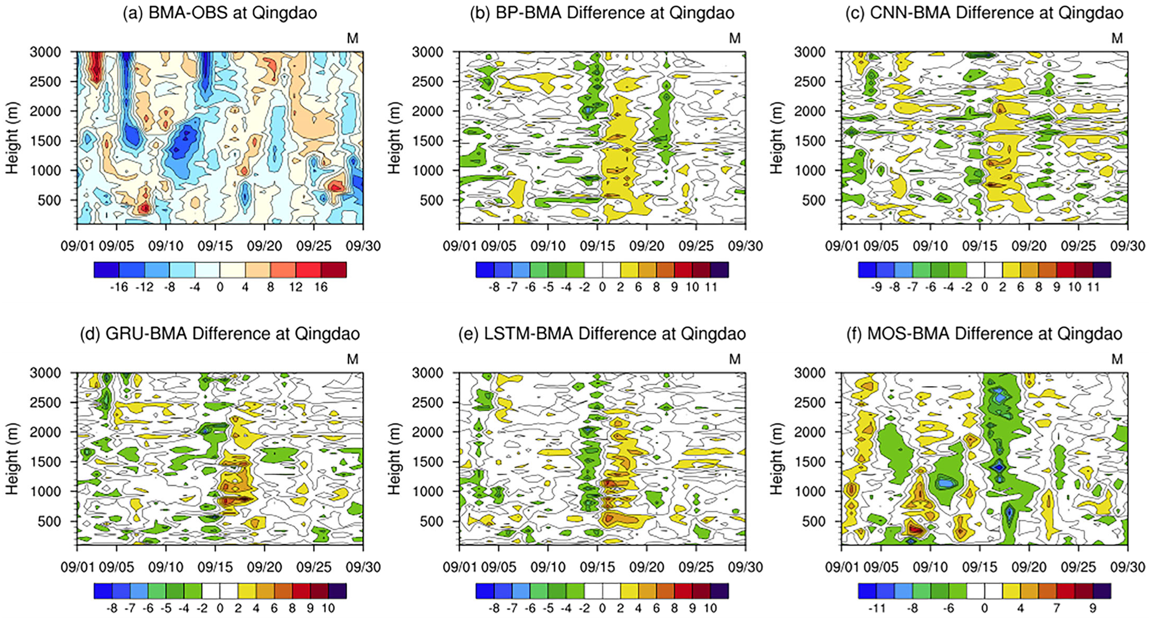
Similarly to Figure 5, Figure 6 and Figure 7 show the bias distributions at the Qingdao and Sheyang stations. Among all three stations, all single correction algorithms exhibited a certain degree of systematic bias, whereas the BMA-based ensemble method produced a more stable bias distribution. In particular, during extreme weather events such as the typhoon passage, the BMA method showed stronger robustness, maintaining good consistency across different height layers and effectively avoiding the height-dependent systematic biases that may occur with single-algorithm corrections.
In terms of the differences among ensemble members, the four neural-network-based algorithms exhibited generally consistent performance with minor variations. On average, the T1_LSTM test produced the lowest overall bias and was the most consistent with the final ensemble result (T1_BMA). Although the T1_MOS test had a relatively higher ME, its distinctive characteristics effectively reduced the uncertainty of the ensemble forecasting under extreme weather conditions. During the simulation period, the RMSE of the T1_BMA ensemble bias-corrected forecasting decreased by 8%, 28%, and 96% compared with the poorest single algorithm member (T1_MOS) at Dalian, Qingdao, and Sheyang stations, respectively.

4.3. Comparison of Accuracy Differences Among Different Ensemble Methods

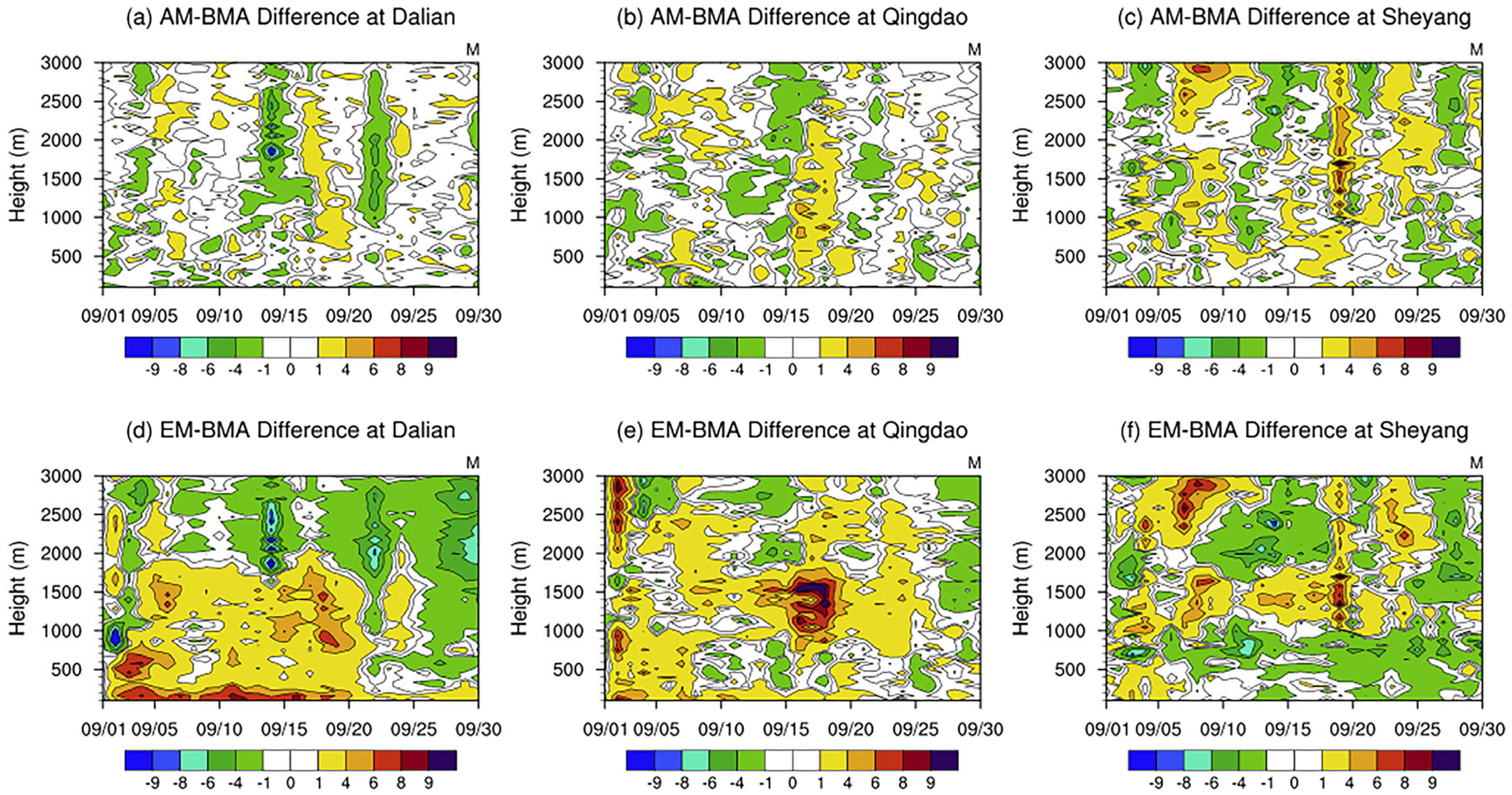
To evaluate the performance differences between the BMA-based ensemble method and other ensemble methods, this study also compared the results of the T1_BMA test with those of T2_AM and T3_EM tests. Figure 8 shows the two-dimensional time–height diagrams of differences between the T1_BMA test and the other two ensemble tests at different altitudes at the Dalian, Qingdao, and Sheyang stations. Figure 8a–c show the difference distributions between the T2_AM and T1_BMA tests (T2_AM − T1_BMA) within the 3000 m altitude range, while Figure 8d–f show the difference distributions between the T3_EM and T1_BMA tests (T3_EM − T1_BMA).
As shown in Figure 8a–c, the differences between the T2_AM and T1_BMA tests at the Dalian and Qingdao stations are relatively small. The distributions of differences between T2_AM and T1_BMA tests were consistent with the color variations in forecasting biases in Figure 5a, Figure 6a and Figure 7a (T1_BMA − OBS). The spatial CCs between Figure 8a–c and Figure 5a, Figure 6a and Figure 7a were 0.37, 0.36, and 0.28, respectively, all positive values. This indicated that, for most of the period, the forecasting biases of the T2_AM test were higher than those of T1_BMA test. For example, during the typhoon passage (15–16 September), the T1_BMA test in Figure 5a and Figure 6a showed a pronounced negative bias, and Figure 8a,b displayed similar negative values for the same event, suggesting that the bias in the T2_AM test was more pronounced than that in the T1_BMA test. At Sheyang Station (Figure 8c), large positive deviations occurred mainly between 1000 m and 2500 m around 19 September and between 2500 m and 3000 m around 8 September, corresponding to the positive biases of T1_BMA in Figure 7a, further confirming that T1_BMA achieved higher simulation accuracy. Overall, under extreme weather conditions, the forecasting accuracy of the T2_AM test significantly decreased, whereas the BMA-based ensemble method in the T1_BMA test achieved more reasonable weight allocation through Bayesian optimization, effectively improving forecasting performance and exhibiting stronger robustness and adaptability.
Figure 8d–f show the differences between the T3_EM and T1_BMA tests. Owing to the dynamic weight adjustment, the overall bias of the T3_EM test was lower than that of the T2_AM test, but it still did not reach the accuracy level of T1_BMA test. The CC between Figure 8d–f and Figure 5a, Figure 6a and Figure 7a were 0.10, 0.20, and 0.18, respectively, all positive values but smaller than those of Figure 8a–c. This indicated that, unlike T2_AM test, the T3_EM test did not substantially amplify the T1_BMA forecasting biases. In terms of temporal distribution, the difference distribution of T3_EM and T1_BMA tests did not align with the bias distribution of T1_BMA.
To provide a clearer comparison among the three ensemble schemes, Table 1 summarized the performance indices of T1_BMA, T2_AM, and T3_EM tests. Among the three approaches, the T1_BMA test achieved the lowest RMSEs and MEs, and the highest CCs. The statistical analysis showed that the RMSE of the T1_BMA test was reduced by approximately 9%, 13%, and 17% compared with the T3_EM test, and by about 9%, 10%, and 14% compared with the T2_AM test at the three stations. These results further confirmed the advantage of the BMA-based ensemble method over other methods under complex weather conditions.
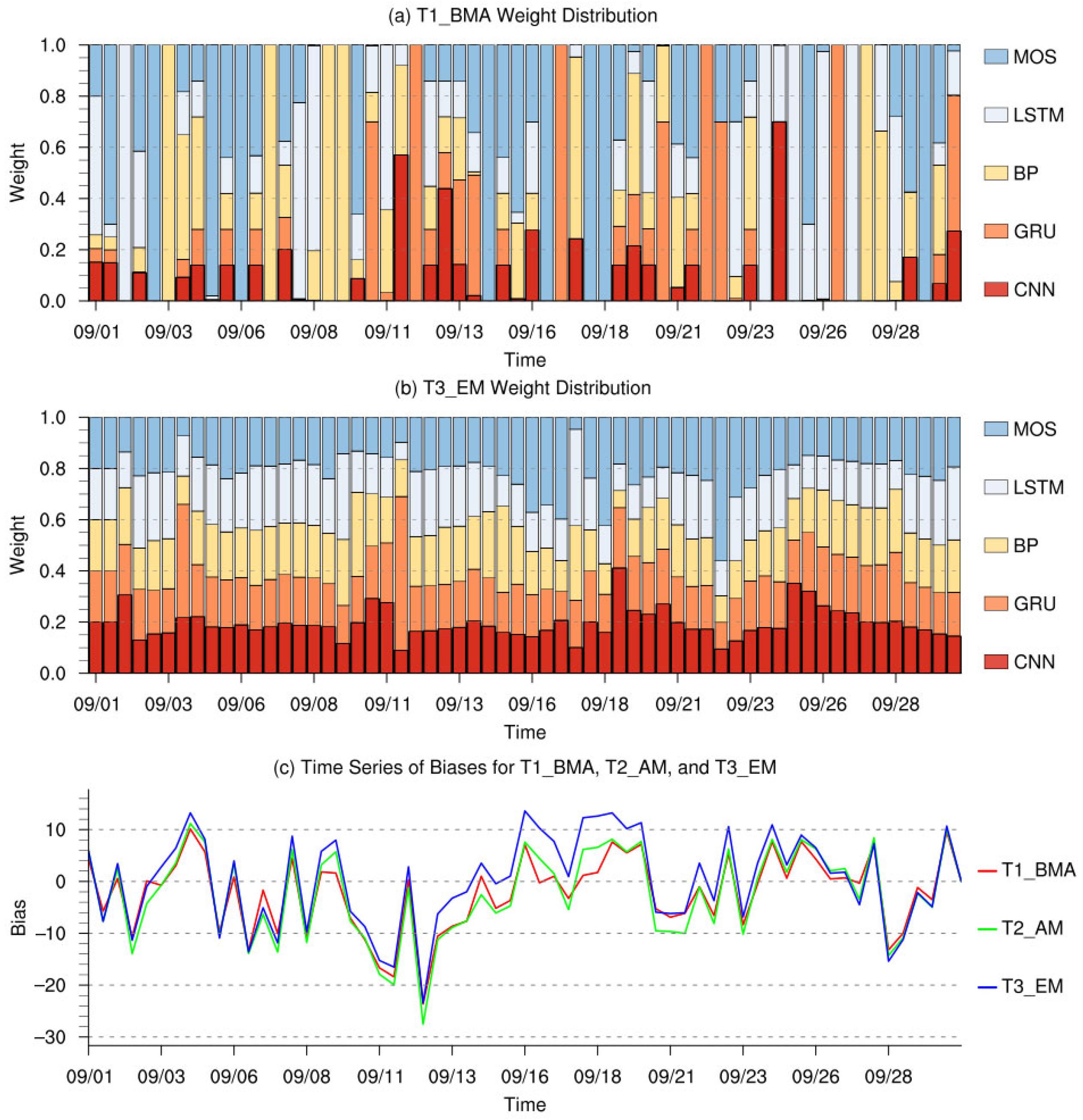
To further investigate the differences in the forecasting performance of the T1_BMA test, this study examined the temporal variations in the weights assigned to the five ensemble members. Since the forecasting result exhibited different behaviors across stations and altitudes, the forecasting result at 1342 m altitude of Qingdao station, where the discrepancies were most pronounced, was selected for analysis.
Figure 9 shows the temporal variations in the weights for the five ensemble members at the 1342 m altitude of Qingdao Station. Among them, Figure 9a shows the weight variations in each ensemble member in the T1_BMA test. The T2_AM test is not displayed because all member weights are fixed at 20%. Figure 9b shows the weight variations in each ensemble member in the T3_EM test. For ease of comparison, Figure 9c provides the time series of forecasting biases for the T1_BMA, T2_AM, and T3_EM tests at this height.
As shown in Figure 9a, the model with the highest weight (close to 1.0) changed almost daily or every few days. When the weight of one model surged above 0.8, the weights of the other models simultaneously dropped sharply to nearly zero. Specifically, the BP, LSTM, and GRU models frequently reached or approached a weight of 1.0. For example, the BP and LSTM models dominated in early and late September, while the GRU model exhibited outstanding performance in mid-September, indicating that these models held transient advantages for certain types of forecasting tasks. In contrast, the MOS model, as a traditional statistical method, achieved the highest weights at several time points (e.g., 6 September and 16 September), further confirming that simple statistical models were also able to provide the highest reliability under extreme weather conditions. On the other hand, the CNN model generally maintained relatively low weights, mostly between 0.0 and 0.2, but also reached its peak on 24 September, suggesting its unique contribution in handling specific nonlinear or complex situations. Overall, these dynamic weight variations revealed that different models exhibited distinct forecasting performance across weather types and temporal stages. The BMA method captured these differences in real time, dynamically adjusting posterior probabilities based on model performance and adaptively assigning higher weights to the best-performing model each day, and thereby achieved an optimized ensemble forecasting result.
As shown in Figure 9b, compared with the weight series in the T1_BMA test, the weight distributions of the models in the T3_EM test were relatively uniform and smooth, with most values fluctuating around 0.2. This smoothness stemmed from the fact that the T3_EM test reflected only the average performance of the previous day, ignoring fluctuations in model performance caused by temporal and meteorological variability, and thus failing to capture sudden changes in model behavior in real time.
Figure 9c shows the temporal series of forecasting biases for the three ensemble methods (T1_BMA, T2_AM, and T3_EM). The closer the curve was to the zero line (bias = 0), the higher the forecasting accuracy. At most time points, the bias curve of the T1_BMA test was the closest to the zero line, indicating a sustained forecasting advantage. This advantage became particularly evident during extreme weather conditions (around 15 September), when the absolute biases of the T1_BMA test were significantly smaller than those of the T2_AM test and T3_EM test. These results further confirm that the BMA method effectively identifies and reduces the influence of underperforming models under extreme weather conditions, thereby demonstrating superior adaptability.

4.4. Bias Statistics of the 48 h and 72 h Forecasting for the Modified Atmospheric Refractivity

In addition to the 24 h ahead forecasting evaluation, Table 2 presents the 48 h ahead and 72 h ahead forecasting indices of the T1_BMA test at the Dalian, Qingdao, and Sheyang stations, along with the corresponding 48 h and 72 h ahead forecasting results from the CTL test for comparison.
As shown in Table 2, the forecasting biases for the 48 h and 72 h ahead lead times were generally consistent with those of the 24 h ahead forecasting, showing no significant change with the extension of forecasting lead time. Among them, the RMSE of the 72 h ahead forecasting was the largest, but it was only 0.35~2.02 M higher than that of the 48 h ahead forecasting, indicating that although the model forecasting biases increased slightly with lead time, they remained at a relatively low level within the 72 h forecasting time range.
Overall, the forecasting accuracy of the T1_BMA test for the 48 h and 72 h ahead forecasting did not show a noticeable decline with the extension of forecasting lead time. At all three stations, the major statistical indices of the T1_BMA test outperformed those of the CTL test. Compared with the 24 h forecasting result, the average RMSE of the T1_BMA test improved by approximately 8%~36% for the 48 h ahead forecasting and by 14%~48% for the 72 h ahead forecasting, while the average CC decreased by around 0.03 and 0.05, respectively.

5. Discussion and Conclusions

Based on the COAWST model, this study developed an atmospheric refractivity forecasting framework that incorporated ensemble bias correction by combining five correction algorithms—BP, CNN, GRU, LSTM, and MOS—with the BMA method. The bias-correction training was conducted using historical simulations of COAWST and radiosonde observation data from 1 January 2016 to 31 December 2021, with the validation period spanning 1–30 September 2022. Several comparative tests were conducted over the Yellow Sea and Bohai Sea regions, including the CTL test using the original COAWST forecasting, the T1 test group employing different bias-correction algorithms (T1_BP, T1_CNN, T1_GRU, T1_LSTM, T1_MOS, and the BMA-based ensemble method T1_BMA), the T2_AM test using an arithmetic average to combine the five bias-corrected forecasting results, and the T3_EM test using a simple variable-weight ensemble averaging method.
The results demonstrated that, compared with single bias-correction algorithms and other ensemble average tests, the BMA-based ensemble method (T1_BMA) maintained higher forecasting accuracy and stability under various weather conditions, significantly improving the forecasting performance of atmospheric refractivity.
However, while the proposed framework demonstrated promising results, several critical issues regarding the BMA methodology and limitations in the experimental design remain to be addressed. These are discussed below in two main aspects.
Although the BMA method effectively reduced inter-model uncertainty, the simulation results revealed several intrinsic limitations within its dynamic weighting mechanism that required further improvement:
  • Lagged response of dynamic weights: The BMA weights were updated based on a sliding window of historical performance. As a consequence, when weather regimes shifted abruptly (e.g., during the rapid passage of a cold front or typhoon), the weight distribution exhibited a lagged response and failed to adjust instantaneously to the current atmospheric state. Future work could incorporate an adaptive sliding-window strategy or a weather-regime recognition module. By dynamically adjusting the window length in response to changes in atmospheric stability, the ensemble framework could respond more rapidly to fast weather transitions.
  • Variance smoothing effect: As indicated by the reduced SD in our results (see Conclusion 2), the BMA method, being a weighted-averaging approach, tended to smooth the prediction variance. While this characteristic helped reduce the RMSE, it may have underestimated extreme values or sharp gradients in the refractivity profile—features that are crucial for identifying strong ducting events. A potential improvement would be to extend the framework from deterministic forecasts to probabilistic predictions. By employing frequency-matching post-processing techniques, future systems could better preserve statistical variance and capture extreme ducting phenomena.
  • Dependency on ensemble bias characteristics: The BMA method relied on the assumption that the true state lay within the spread of the ensemble members. In cases where all models systematically overestimated or underestimated the observations (e.g., due to structural deficiencies in the COAWST boundary-layer parameterization), the weighted-averaging mechanism struggled to correct the bias effectively. Therefore, enhancing the diversity of ensemble members was essential. Future research would explore integrating heterogeneous models driven by different physical parameterization schemes to expand the ensemble spread.
Uncertainties also arose from the current algorithm, result, and experimental design, pointing to specific directions for future improvement:
  • As for the bias correction algorithm aspect, regarding the selection of bias correction algorithms, this study primarily employed classical deep learning models (e.g., CNN, LSTM). To rigorously justify the computational cost associated with these complex algorithms, we conducted additional comparative tests using traditional statistical models, specifically ARIMA and Linear Regression (LR), as benchmarks (see Table 3). The results indicated that the deep learning-based methods consistently outperformed these simpler statistical models in terms of RMSE and CCs, confirming that their ability to capture non-linear error patterns justified the increased complexity. However, even the advanced deep learning models did not yield optimal performance across all weather scenarios, as their accuracy largely depended on the specific feature-capturing capabilities and training strategies. This inconsistency reinforced the necessity of the dynamic ensemble weighting strategy (BMA) adopted in this study to mitigate algorithmic uncertainty. Future work will focus on two aspects to further enhance model performance: first, exploring state-of-the-art architectures such as Transformer networks and attention mechanisms, which have shown superior potential in handling long-term dependencies compared to RNNs, and second, optimizing the training strategy by incorporating advanced data preprocessing techniques. Previous studies demonstrated that applying data clustering, Principal Component Analysis (PCA), and other feature extraction methods can significantly improve model robustness, an aspect not yet addressed in the present study but planned for future investigation.
2.
As for the result aspect, the validation data used in this study also had representativeness limitations. Because the ERA5 data with certain biases was not suitable as the evaluation reference in this study, only radiosonde observation data from three stations were selected for the verification of atmospheric duct characteristics, and the choice of stations was somewhat random. Furthermore, the radiosonde observation data were available only twice daily and occasionally contained missing values, highlighting the need for collecting denser and more continuous observations for future validation and assessment. In addition, this study used only the modified atmospheric refractivity series output from the COAWST model as input to the neural networks, without incorporating fundamental meteorological variables such as air temperature, air pressure, and humidity. This represented an underutilization of the COAWST model’s available information. Atmospheric ducts are physically driven by vertical gradients of temperature and humidity. By excluding these available meteorological variables and relying solely on univariate error history, the machine learning models essentially performed advanced signal smoothing rather than learning the physical error correlations, which limited the intelligence of the bias correction. Future studies will consider developing a multidimensional feature framework that includes complete meteorological fields (e.g., temperature profiles, pressure fields, humidity fields, and wind fields) and integrating physical constraints into the neural network construction process, with the goal of enhancing the model’s physical interpretability while maintaining strong statistical performance.
3.
As for the experimental design aspect, the training period (January 2016 to December 2021) and validation period (September 2022) were not consecutive. However, this design was driven by specific scientific considerations. First, to rigorously test the model’s generalization capability, this study intentionally selected a “future” and “unseen” period distinct from the training set, rather than using random cross-validation. This approach cuts off the temporal “memory” inherent in meteorological data, thereby simulating a realistic operational forecasting scenario where the model must perform without prior knowledge. Second, the selection of September 2022 as this period featured the rare passage of Typhoon Muifa, which passed the study domain from south to north, providing a unique opportunity to evaluate error performance under extreme atmospheric perturbations. Additionally, as a seasonal transition period characterized by the retreat of the East Asian summer monsoon and alternating cold/warm fronts, September represents a critical window for atmospheric duct formation. Third, although the duration was short, the experiment involved daily rolling forecasts for the next 72 h, generating a substantial volume of hourly evaluation points equivalent to three months of data. Nevertheless, the one-month duration is not sufficient enough to comprehensively evaluate the model’s long-term applicability across different seasonal patterns and inter-annual variations. Future work will prioritize conducting longer-term and continuous forecasting tests to further verify the robustness and optimize the performance of the proposed framework.
The main conclusions of this study are as follows:
  • During the validation period in September 2022, comparison with radiosonde observation data at the Dalian, Qingdao, and Sheyang stations showed that the COAWST model exhibited relatively high RMSEs of the modified atmospheric refractivity forecasting below 1000 m, with the overall bias decreased with increasing altitude. After applying the BMA-based ensemble bias correction, the forecasting result of modified atmospheric refractivity outperformed the original COAWST model forecasting in terms of RMSE, ME, and CC. In addition, the RMSE of the BMA-corrected forecasting was lower than that of the ERA5 data, although the CC was slightly lower.
  • After BMA-based ensemble bias correction, the CC between the forecasting result and radiosonde observation data increased by 0.04, 0.05, and 0.06, respectively. However, the SD of the corrected forecasting was lower than that of the original model, which was consistent with previous studies, indicating that the BMA-based ensemble bias correction reduced the variability of the forecasting series to some extent.
  • Regarding the differences among ensemble members, the four neural-network-based algorithm members exhibited varying degrees of systematic bias during the typhoon passage. On average, the T1_LSTM test showed the lowest overall biases. The unique diversity of the T1_MOS test played a compensatory role within the ensemble, effectively reducing the uncertainty of the BMA-based ensemble method.
  • In terms of the performance of different ensemble methods, the arithmetic average (T2_AM) test and variable-weight ensemble averaging (T3_EM) method failed to capture nonlinear bias characteristics under extreme conditions, resulting in lower forecasting accuracy than the T1_BMA test. This finding further confirmed that the BMA-based ensemble method, through Bayesian optimization, effectively achieved adaptive weight allocation, allowing it to balance the contributions of single models more accurately under complex weather conditions.
  • From the perspective of different forecasting result lead times, the T1_BMA test effectively reduced both systematic and random biases and improved correlations with radiosonde observation data in the 72-h forecasting. These results indicated that the ensemble bias correction model developed in this study was able to maintain high stability and adaptability in short-term forecasting applications.

Author Contributions

Writing—review and editing, J.Z.; methodology, B.W. (Bo Wang); software, X.Z.; validation, Z.Q. and H.W. (Hanyue Wang); resources, L.L., X.L. and H.W. (Hang Wang); supervision, X.L.; conceptualization, B.W. (Bin Wang); writing—original draft preparation, H.G. All authors have read and agreed to the published version of the manuscript.

Funding

This study was financially supported by the National Key Research and Development Program of China (2022YFC3104202), the Shandong Provincial Key Research and Development Program project (2023CXPT015), the National Natural Science Foundation of China (42206188, 42176185), the Natural Science Foundation of Shandong province, China (ZR2022MD100), and the basic research foundation (2024GH05, 2025ZDZX05, 2025ZDYS01, 2025ZDGZ01, 2023JBZ02, 2023JBZ01) of Qilu University of Technology.

Data Availability Statement

The data used in this study is not publicly available due to internal policy of Qilu University of Technology, and is available from the corresponding author upon request.

Conflicts of Interest

The authors declare no conflicts of interest.

Abbreviations

The following abbreviations are used in this manuscript:
COAWSTCoupled Ocean–Atmosphere–Wave–Sediment Transport
BMABayesian Model Averaging
MEMean Error
RMSERoot Mean Square Error
CCCorrelation Coefficient
AIArtificial Intelligence
RKHSReproducing Kernel Hilbert Space
EnKFEnsemble Kalman Filter
SPCAMSuper Parameterized Community Atmosphere Model
NNCAMNeural Network version of Community Atmosphere Model
ECMWFEuropean Centre for Medium-Range Weather Forecast
IFSIntegrated Forecasting System
ANOAnomaly Numerical-correction with Observations
WRFWeather Research and Forecasting
Bi-LSTMBidirectional Long Short-Term Memory
TrajGRUTrajectory Gated Recurrent Unit
RERelative Error
MAEMean Absolute Error
ERA5ECMWF Reanalysis v5
CNNConvolutional Neural Network
LSTMLong Short-Term Memory
GRUGated Recurrent Unit
BPBackpropagation Neural Network
MOSModel Output Statistics
ROMSRegional Ocean Modeling System
SWANSimulating Waves Nearshore
MCTModel Coupling Toolkit
1-D CNNOne-dimensional convolutional neural network
MCMCMarkov Chain Monte Carlo
WSM6WRF Single-Moment 6-Class
MM5The fifth-Generation Penn State/NCAR Mesoscale Model
RRTMRapid Radiative Transfer Model
Noah-LSMNoah Land Surface Model
GFGrell–Freitas
GFSGlobal Forecast System
RTOFSReal Time Ocean Forecast System
PCAPrincipal component analysis
NCEPNational Centers for Environmental Prediction
GDASGlobal Data Assimilation System
GOFSGlobal Ocean Forecasting System
PDFProbability Density Function
WRF-3DVarThree-Dimensional Variational Assimilation Module
LRLinear Regression
MSEMean Squared Error
WPSWRF Preprocessing System
MModified Atmospheric Refractivity
NRefractivity
TAir Temperature
PAir Pressure
eWater Vapor Pressure
qSpecific Humidity
ε0.622
HAltitude
yForecasting Variable
fBias-correction Model Space
KNumber of Models
DObservation Dataset
p k ( y | f k , D ) Conditional PDF of the Forecasting Variable
p ( f k | D ) Posterior Probability of the kth Model
p ( D | f j ) Marginal or Integrated Likelihood of Each Model
θ j Parameter Vector of Model
σ k 2   Variance
μ k Expected Value
Mens,dtEnsemble Forecasting for Day d at Time t
Od−1Observations on the Previous Day d − 1
iForecasting Member ID
NTotal Number of Forecasting Members
αi,dWeight of Model Mi on Day d
EReciprocal of the RMSE

References

  1. Wang, H.; Su, S.; Tang, H.; Jiao, L.; Li, Y. Atmospheric Duct Detection Using Wind Profiler Radar and RASS. J. Atmos. Ocean. Technol. 2019, 36, 557–565. [Google Scholar] [CrossRef]
  2. Thompson, W.T.; Haack, T. An Investigation of Sea Surface Temperature Influence on Microwave Refractivity: The Wallops-2000 Experiment. J. Appl. Meteorol. Climatol. 2011, 50, 2319–2337. [Google Scholar] [CrossRef]
  3. Babin, S.M.; Young, G.S.; Carton, J.A. A New Model of the Oceanic Evaporation Duct. J. Appl. Meteorol. 1997, 36, 193–204. [Google Scholar] [CrossRef]
  4. Dinc, E.; Akan, O. Beyond-Line-of-Sight Communications with Ducting Layer. IEEE Commun. Mag. 2014, 52, 37–43. [Google Scholar] [CrossRef]
  5. Dinc, E.; Akan, O.B. Channel Model for the Surface Ducts: Large-Scale Path-Loss, Delay Spread, and AOA. IEEE Trans. Antennas Propagat. 2015, 63, 2728–2738. [Google Scholar] [CrossRef]
  6. Zhang, Y.; Guo, X.; Zhao, Q.; Zhao, Z.; Kang, S. Research status and thinking of atmospheric duct. Chin. J. Radio Sci. 2020, 35, 813–831. [Google Scholar] [CrossRef]
  7. Brownlee, K.A. Statistical Theory and Methodology in Science and Engineering; John Wiley Sons Wiley: New York, NY, USA, 1965; pp. 26–30. [Google Scholar]
  8. Yao, Z.; Zhao, B.; Li, W.; Zhu, Y.; Du, J.; Dai, F. The analysis on characteristic of atmospheric duct and its effects on the propagation of electromagnetic wave. Acta Meteorol. Sin. 2000, 58, 605–616. [Google Scholar] [CrossRef]
  9. Ren, L.; Hu, Z.; Hartnett, M. Short-Term Forecasting of Coastal Surface Currents Using High Frequency Radar Data and Artificial Neural Networks. Remote Sens. 2018, 10, 850. [Google Scholar] [CrossRef]
  10. Kim, M.; Yang, H.; Kim, J. Sea Surface Temperature and High Water Temperature Occurrence Prediction Using a Long Short-Term Memory Model. Remote Sens. 2020, 12, 3654. [Google Scholar] [CrossRef]
  11. Berry, T.; Harlim, J. Correcting Biased Observation Model Error in Data Assimilation. Mon. Weather Rev. 2017, 145, 2833–2853. [Google Scholar] [CrossRef]
  12. Rasp, S.; Pritchard, M.S.; Gentine, P. Deep Learning to Represent Subgrid Processes in Climate Models. Proc. Natl. Acad. Sci. USA 2018, 115, 9684–9689. [Google Scholar] [CrossRef]
  13. Han, L.; Chen, M.; Chen, K.; Chen, H.; Zhang, Y.; Lu, B.; Song, L.; Qin, R. A Deep Learning Method for Bias Correction of ECMWF 24–240 h Forecasts. Adv. Atmos. Sci. 2021, 38, 1444–1459. [Google Scholar] [CrossRef]
  14. Yao, N.; Ye, J.; Wang, S.; Yang, S.; Lu, Y.; Zhang, H.; Yang, X. Bias Correction of the Hourly Satellite Precipitation Product Using Machine Learning Methods Enhanced with High-Resolution WRF Meteorological Simulations. Atmos. Res. 2024, 310, 107637. [Google Scholar] [CrossRef]
  15. Zhang, W.; Sun, Y.; Wu, Y.; Dong, J.; Song, X.; Gao, Z.; Pang, R.; Guoan, B. A Deep-Learning Real-Time Bias Correction Method for Significant Wave Height Forecasts in the Western North Pacific. Ocean Modell. 2024, 187, 102289. [Google Scholar] [CrossRef]
  16. Huang, H.; Liang, Z.; Li, B.; Wang, D.; Hu, Y.; Li, Y. Combination of Multiple Data-Driven Models for Long-Term Monthly Runoff Predictions Based on Bayesian Model Averaging. Water Resour. Manag. 2019, 33, 3321–3338. [Google Scholar] [CrossRef]
  17. Rasp, S.; Lerch, S. Neural Networks for Postprocessing Ensemble Weather Forecasts. Mon. Weather Rev. 2018, 146, 3885–3900. [Google Scholar] [CrossRef]
  18. Leutbecher, M.; Palmer, T.N. Ensemble Forecasting. J. Comput. Phys. 2008, 227, 3515–3539. [Google Scholar] [CrossRef]
  19. Maqsood, I.; Khan, M.; Abraham, A. An Ensemble of Neural Networks for Weather Forecasting. Neural Comput. Appl. 2004, 13, 112–122. [Google Scholar] [CrossRef]
  20. McLean Sloughter, J.; Gneiting, T.; Raftery, A.E. Probabilistic Wind Vector Forecasting Using Ensembles and Bayesian Model Averaging. Mon. Weather Rev. 2013, 141, 2107–2119. [Google Scholar] [CrossRef]
  21. Achite, M.; Banadkooki, F.B.; Ehteram, M.; Bouharira, A.; Ahmed, A.N.; Elshafie, A. Exploring Bayesian Model Averaging with Multiple ANNs for Meteorological Drought Forecasts. Stoch. Environ. Res. Risk Assess. 2022, 36, 1835–1860. [Google Scholar] [CrossRef]
  22. Duan, Q.; Ajami, N.K.; Gao, X.; Sorooshian, S. Multi-Model Ensemble Hydrologic Prediction Using Bayesian Model Averaging. Adv. Water Resour. 2007, 30, 1371–1386. [Google Scholar] [CrossRef]
  23. Li, G.; Liu, Z.; Zhang, J.; Han, H.; Shu, Z. Bayesian Model Averaging by Combining Deep Learning Models to Improve Lake Water Level Prediction. Sci. Total Environ. 2024, 906, 167718. [Google Scholar] [CrossRef]
  24. Liu, Q.; Zhao, X.; Zou, J.; Li, Y.; Qiu, Z.; Hu, T.; Wang, B.; Li, Z. Development of a Numerical Prediction Model for Marine Lower Atmospheric Ducts and Its Evaluation across the South China Sea. J. Mar. Sci. Eng. 2024, 12, 141. [Google Scholar] [CrossRef]
  25. Long, M.; Yu, K.; Lu, Y.; Wang, S.; Tang, J. High Resolution Regional Climate Simulation over CORDEX East Asia Phase II Domain Using the COAWST Ocean-Atmosphere Coupled Model. Clim. Dyn. 2024, 62, 8711–8727. [Google Scholar] [CrossRef]
  26. Warner, J.C.; Armstrong, B.; He, R.; Zambon, J.B. Development of a Coupled Ocean-Atmosphere-Wave-Sediment Transport (COAWST) Modeling System. Ocean Modell. 2010, 35, 230–244. [Google Scholar] [CrossRef]
  27. Rumelhart, D.E.; Hinton, G.E.; Williams, R.J. Learning Representations by Back-Propagating Errors. Nature 1986, 323, 533–536. [Google Scholar] [CrossRef]
  28. Venkatesan, C.; Raskar, S.D.; Tambe, S.S.; Kulkarni, B.D.; Keshavamurty, R.N. Prediction of All India Summer Monsoon Rainfall Using Error-Back-Propagation Neural Networks. Meteorol. Atmos. Phys. 1997, 62, 225–240. [Google Scholar] [CrossRef]
  29. Lee, T.-L. Back-Propagation Neural Network for the Prediction of the Short-Term Storm Surge in Taichung Harbor, Taiwan. Eng. Appl. Artif. Intell. 2008, 21, 63–72. [Google Scholar] [CrossRef]
  30. Lee, T.-L. Back-Propagation Neural Network for Long-Term Tidal Predictions. Ocean Eng. 2004, 31, 225–238. [Google Scholar] [CrossRef]
  31. Li, Z.; Liu, F.; Yang, W.; Peng, S.; Zhou, J. A Survey of Convolutional Neural Networks: Analysis, Applications, and Prospects. IEEE Trans. Neural Netw. Learn. Syst. 2022, 33, 6999–7019. [Google Scholar] [CrossRef]
  32. Ince, T.; Kiranyaz, S.; Eren, L.; Askar, M.; Gabbouj, M. Real-Time Motor Fault Detection by 1-D Convolutional Neural Networks. IEEE Trans. Ind. Electron. 2016, 63, 7067–7075. [Google Scholar] [CrossRef]
  33. Cho, K.; van Merrienboer, B.; Gulcehre, C.; Bahdanau, D.; Bougares, F.; Schwenk, H.; Bengio, Y. Learning Phrase Representations Using RNN Encoder-Decoder for Statistical Machine Translation. arXiv 2014, arXiv:1406.1078. [Google Scholar] [CrossRef]
  34. Dutta, A.; Kumar, S.; Basu, M. A Gated Recurrent Unit Approach to Bitcoin Price Prediction. J. Risk Financ. Manag. 2020, 13, 23. [Google Scholar] [CrossRef]
  35. Hochreiter, S.; Schmidhuber, J. Long Short-Term Memory. Neural Comput. 1997, 9, 1735–1780. [Google Scholar] [CrossRef]
  36. Tian, C.; Ma, J.; Zhang, C.; Zhan, P. A Deep Neural Network Model for Short-Term Load Forecast Based on Long Short-Term Memory Network and Convolutional Neural Network. Energies 2018, 11, 3493. [Google Scholar] [CrossRef]
  37. Glahn, H.R.; Lowry, D.A. The Use of Model Output Statistics (MOS) in Objective Weather Forecasting. J. Appl. Meteorol. 1972, 11, 1203–1211. [Google Scholar] [CrossRef]
  38. Raftery, A.E.; Gneiting, T.; Balabdaoui, F.; Polakowski, M. Using Bayesian Model Averaging to Calibrate Forecast Ensembles. Mon. Weather Rev. 2005, 133, 1155–1174. [Google Scholar] [CrossRef]
  39. Bardsley, W.E. Note on the Use of the Inverse Gaussian Distribution for Wind Energy Applications. J. Appl. Meteorol. Climatol. 1980, 19, 1126–1130. [Google Scholar] [CrossRef]
  40. Chen, Y.; Yuan, W.; Xia, J.; Fisher, J.B.; Dong, W.; Zhang, X.; Liang, S.; Ye, A.; Cai, W.; Feng, J. Using Bayesian Model Averaging to Estimate Terrestrial Evapotranspiration in China. J. Hydrol. 2015, 528, 537–549. [Google Scholar] [CrossRef]
  41. Jones, G.L.; Qin, Q. Markov Chain Monte Carlo in Practice. Annu. Rev. Stat. Appl. 2022, 9, 557–578. [Google Scholar] [CrossRef]
  42. Li, G.; Shi, J. Application of Bayesian Model Averaging in Modeling Long-Term Wind Speed Distributions. Renew. Energy 2010, 35, 1192–1202. [Google Scholar] [CrossRef]
  43. Sorooshian, S.; Dracup, J.A. Stochastic Parameter Estimation Procedures for Hydrologie Rainfall-runoff Models: Correlated and Heteroscedastic Error Cases. Water Resour. Res. 1980, 16, 430–442. [Google Scholar] [CrossRef]
  44. Yi, D.; Ahn, J.; Ji, S. An Effective Optimization Method for Machine Learning Based on ADAM. Appl. Sci. 2020, 10, 1073. [Google Scholar] [CrossRef]
  45. Yao, Y.; Rosasco, L.; Caponnetto, A. On Early Stopping in Gradient Descent Learning. Constr. Approx. 2007, 26, 289–315. [Google Scholar] [CrossRef]
  46. Zang, T.; Zou, J.; Li, Y.; Qiu, Z.; Wang, B.; Cui, C.; Li, Z.; Hu, T.; Guo, Y. Development and Evaluation of a Short-Term Ensemble Forecasting Model on Sea Surface Wind and Waves across the Bohai and Yellow Sea. Atmosphere 2024, 15, 197. [Google Scholar] [CrossRef]
  47. Haack, T.; Wang, C.; Garrett, S.; Glazer, A.; Mailhot, J.; Marshall, R. Mesoscale Modeling of Boundary Layer Refractivity and Atmospheric Ducting. J. Appl. Meteorol. Climatol. 2010, 49, 2437–2457. [Google Scholar] [CrossRef]
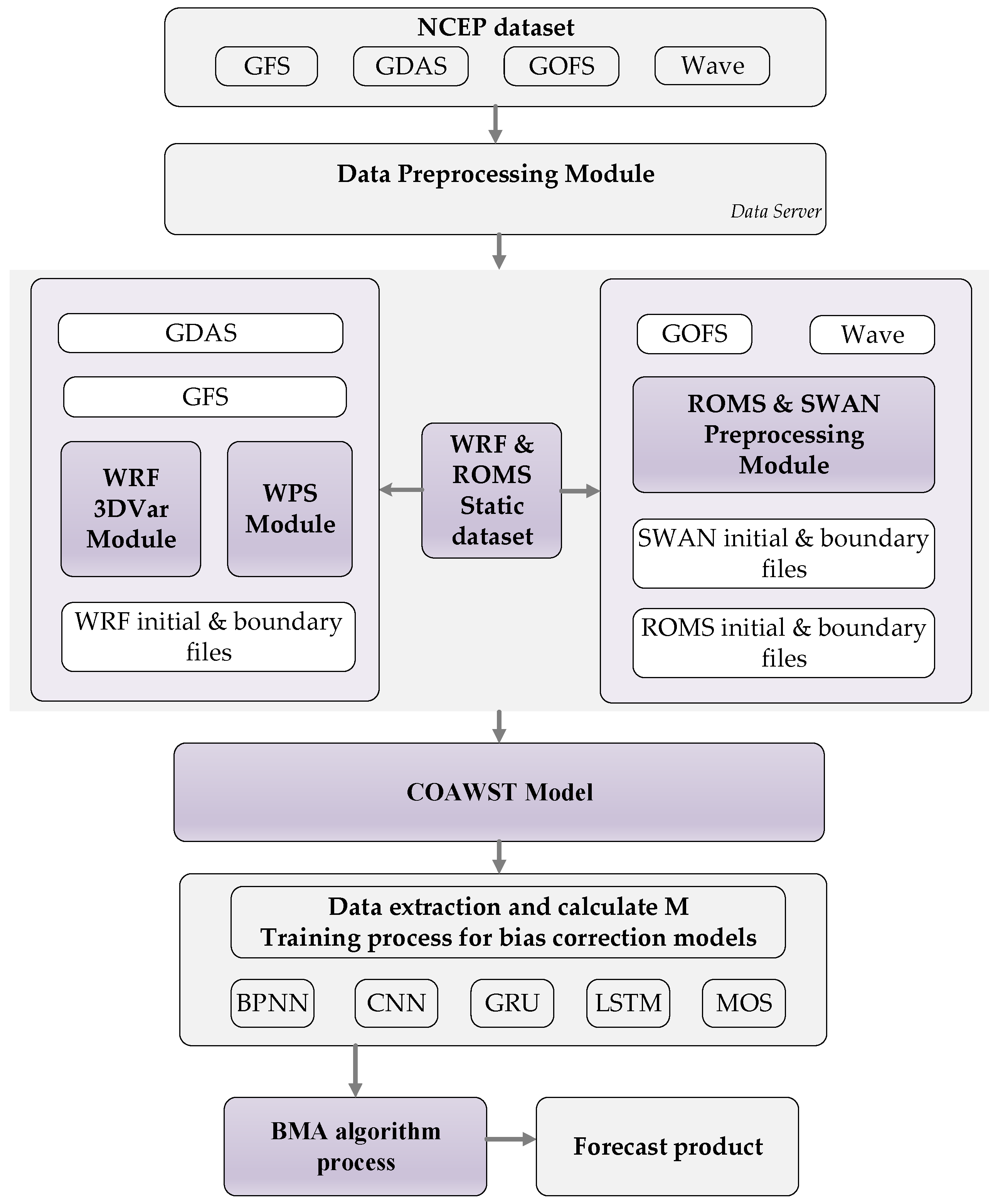
Figure 1. Flowchart of the forecasting system workflow.
Jmse 13 02397 g001
Figure 2. The topography and bathymetry over the study domain. The entire domain is used for the simulation of the WRF component model, and the area enclosed by the red rectangular box indicates the simulation domain of the ROMS and SWAN component models. The black dots represent the locations of the radiosonde stations, and the blue line denotes the track of Typhoon Muifa in the domain, with the blue dots representing the observation of the typhoon center.
Jmse 13 02397 g002
Figure 3. Vertical ME profiles of the modified atmospheric refractivity with height at (a) Dalian, (b) Qingdao, and (c) Sheyang stations; vertical RMSE profiles of the modified atmospheric refractivity with height at (d) Dalian, (e) Qingdao, and (f) Sheyang stations; and vertical CC profiles of the modified atmospheric refractivity with height at (g) Dalian, (h) Qingdao, and (i) Sheyang stations. The red, blue, and green lines represent the T1_BMA test, the CTL test and the ERA5 reanalysis data, respectively.
Jmse 13 02397 g003
Figure 4. Taylor diagrams of the modified atmospheric refractivity for the CTL test, T1_BMA test, and ERA5 data, showing the comparison results with radiosonde observation data at (a) Dalian, (b) Qingdao, and (c) Sheyang stations. The red, blue, and green dots represent the T1_BMA test, the CTL test and the ERA5 reanalysis data, respectively.
Jmse 13 02397 g004
Figure 5. Two-dimensional temporal distributions at different altitudes for (a) 24 h forecasting biases of T1_BMA test (T1_BMA − OBS); (b) differences between T1_BP and T1_BMA tests (T1_BP − T1_BMA); (c) differences between T1_CNN and T1_BMA tests (T1_CNN − T1_BMA); (d) differences between T1_GRU and T1_BMA tests (T1_GRU − T1_BMA); (e) differences between T1_LSTM and T1_BMA tests (T1_LSTM − T1_BMA); (f) differences between T1_MOS and T1_BMA tests (T1_MOS − T1_BMA) at the Dalian station.
Jmse 13 02397 g005
Figure 6. Two-dimensional temporal distributions at different altitudes for (a) 24 h forecasting biases of T1_BMA test (T1_BMA − OBS); (b) differences between T1_BP and T1_BMA tests (T1_BP − T1_BMA); (c) differences between T1_CNN and T1_BMA tests (T1_CNN − T1_BMA); (d) differences between T1_GRU and T1_BMA tests (T1_GRU − T1_BMA); (e) differences between T1_LSTM and T1_BMA tests (T1_LSTM − T1_BMA); (f) differences between T1_MOS and T1_BMA tests (T1_MOS − T1_BMA) at the Qingdao station.
Jmse 13 02397 g006
Figure 7. Two-dimensional temporal distributions at different altitudes for (a) 24 h forecasting biases of T1_BMA test (T1_BMA − OBS); (b) differences between T1_BP and T1_BMA tests (T1_BP − T1_BMA); (c) differences between T1_CNN and T1_BMA tests (T1_CNN − T1_BMA); (d) differences between T1_GRU and T1_BMA tests (T1_GRU − T1_BMA); (e) differences between T1_LSTM and T1_BMA tests (T1_LSTM − T1_BMA); (f) differences between T1_MOS and T1_BMA tests (T1_MOS − T1_BMA) at the Sheyang station.
Jmse 13 02397 g007
Figure 8. Two-dimensional temporal distributions at different altitudes for the 24 h forecasting differences between T1_BMA test and the other two ensemble tests. (a) Dalian Station, (b) Qingdao Station, and (c) Sheyang Station—differences between the T2_AM and T1_BMA tests; (d) Dalian Station, (e) Qingdao Station, and (f) Sheyang Station—differences between the T3_EM and T1_BMA tests.
Jmse 13 02397 g008
Figure 9. Temporal variations in the weights for the five ensemble members at the 1342 m of Qingdao Station in the (a) T1_BMA test and (b) T3_EM test, and (c) the time series of forecasting biases for the T1_BMA, T2_AM, and T3_EM tests.
Jmse 13 02397 g009
Table 1. ME, RMSE, and CC of the T1_BMA, T2_AM and T3_EM tests at the Dalian, Qingdao, and Sheyang stations for the 24 h forecasting ahead.
StationT1_BMAT2_AMT3_EM
MERMSECCMERMSECCMERMSECC
Dalian0.28 M7.51 M0.990.38 M8.27 M0.980.48 M8.29 M0.98
Qingdao−0.14 M7.15 M0.99−0.84 M7.94 M0.980.82 M8.22 M0.99
Sheyang0.03 M6.82 M0.990.25 M7.95 M0.99−0.14 M8.21 M0.99
Table 2. ME, RMSE, and CC of the T1_CTL and T1_BMA tests at the Dalian, Qingdao, and Sheyang stations for the 48 h and 72 h ahead forecasting.
StationForecasting Lead TimeCTLT1_BMA
MERMSECCMERMSECC
Dalian48 h ahead1.99 M11.34 M0.830.94 M8.91 M0.90
72 h ahead1.55 M11.69 M0.810.65 M9.09 M0.89
Qingdao48 h ahead0.20 M11.48 M0.82−0.44 M8.42 M0.89
72 h ahead0.20 M13.50 M0.760.39 M9.34 M0.87
Sheyang48 h ahead3.78 M15.19 M0.771.46 M9.86 M0.89
72 h ahead1.05 M16.03 M0.710.26 M10.73 M0.87
Table 3. RMSE and CC of bias-correction methods including classical statistical baselines at the Dalian, Qingdao, and Sheyang stations for the 24 h ahead forecasting.
IndicesForecasting Lead TimeStationBPCNNGRULSTMMOSLRARIMA
RMSE24 h aheadDalian9.02 M9.44 M9.01 M8.19 M9.25 M9.24 M8.81 M
Qingdao8.30 M8.90 M8.74 M7.74 M9.19 M9.25 M9.19 M
Sheyang8.55 M8.82 M8.51 M7.88 M9.57 M9.70 M9.67 M
CC24 h aheadDalian0.910.890.910.930.890.890.89
Qingdao0.890.870.880.910.860.860.86
Sheyang0.920.910.920.940.880.890.88
Disclaimer/Publisher’s Note: The statements, opinions and data contained in all publications are solely those of the individual author(s) and contributor(s) and not of MDPI and/or the editor(s). MDPI and/or the editor(s) disclaim responsibility for any injury to people or property resulting from any ideas, methods, instructions or products referred to in the content.