Author Contributions
Conceptualization, J.J. and Z.W.; methodology, K.S.; software, K.S.; validation, K.S.; formal analysis, J.G. and R.G.; investigation, Z.W.; resources, Z.W.; data curation, J.J., K.S. and Z.W.; writing—original draft preparation, J.G.; writing—review and editing, R.G.; visualization, K.S.; supervision, J.J.; project administration, Z.W.; funding acquisition, J.J. All authors have read and agreed to the published version of the manuscript.
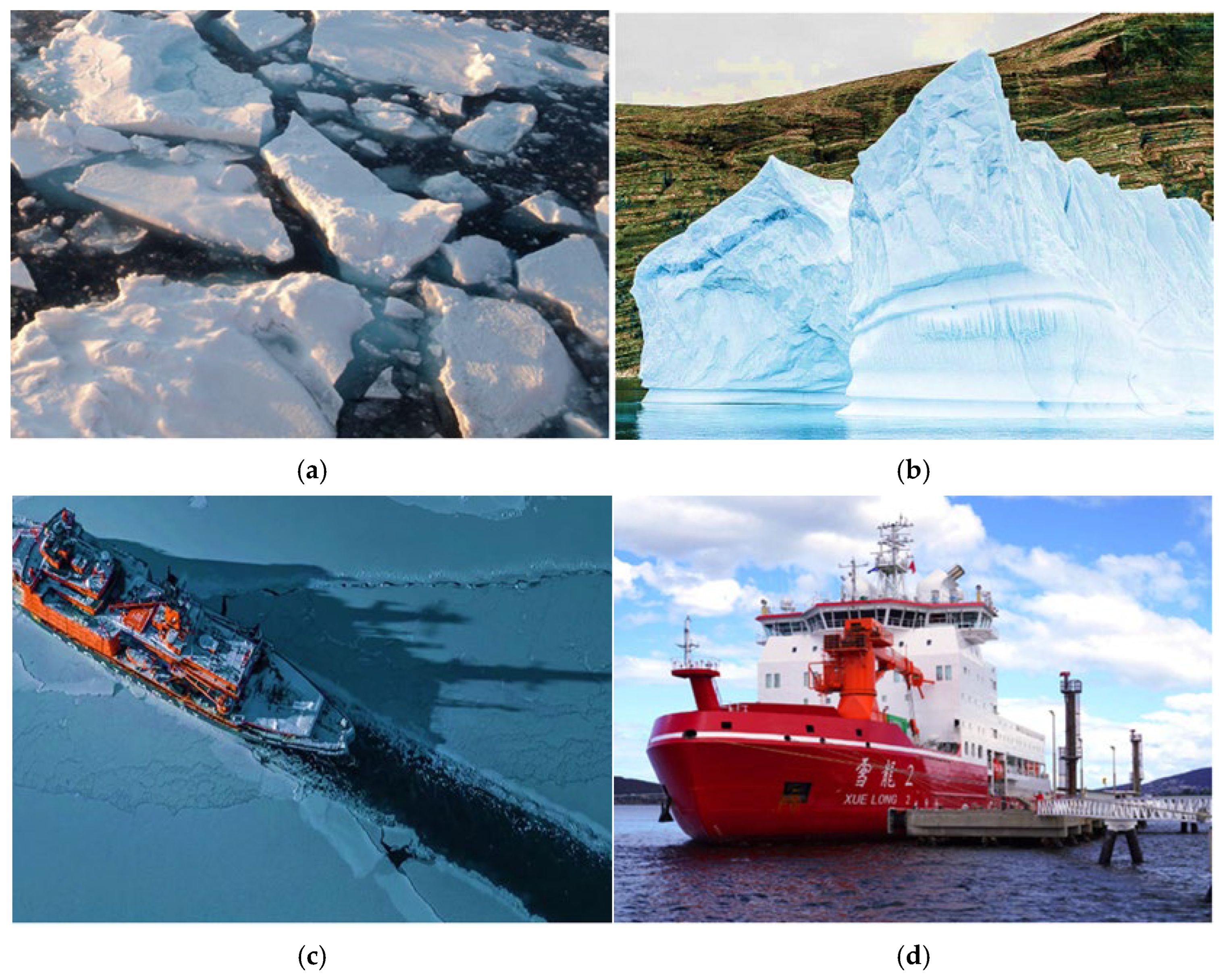
Figure 1.
Four types of polar targets: (a) sea ice image, (b) iceberg image, (c) ice channel, and (d) icebreaker “XUE LONG 2”.
Figure 1.
Four types of polar targets: (a) sea ice image, (b) iceberg image, (c) ice channel, and (d) icebreaker “XUE LONG 2”.
Figure 2.
The structure of convolutional block attention module, where “*” denotes the multiplication operation.
Figure 2.
The structure of convolutional block attention module, where “*” denotes the multiplication operation.
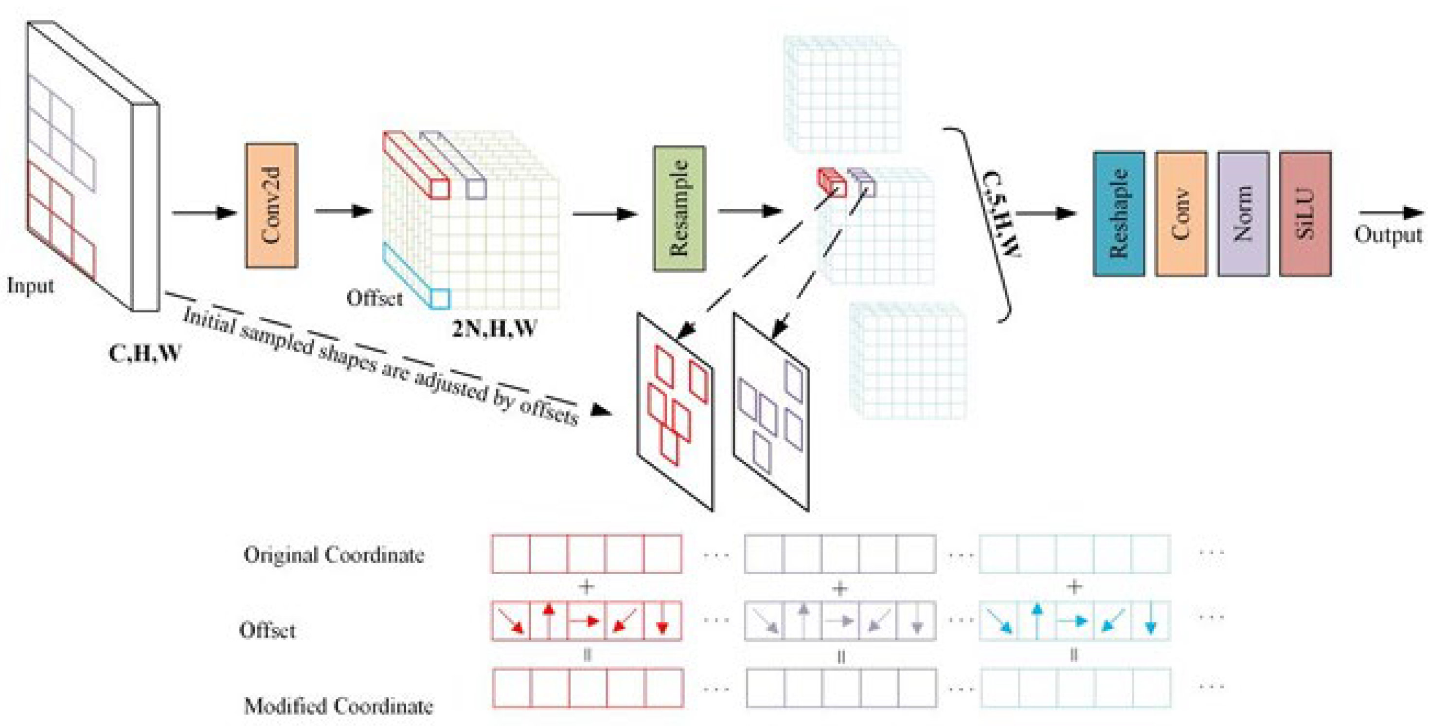
Figure 3.
AKConv convolution diagram.
Figure 3.
AKConv convolution diagram.
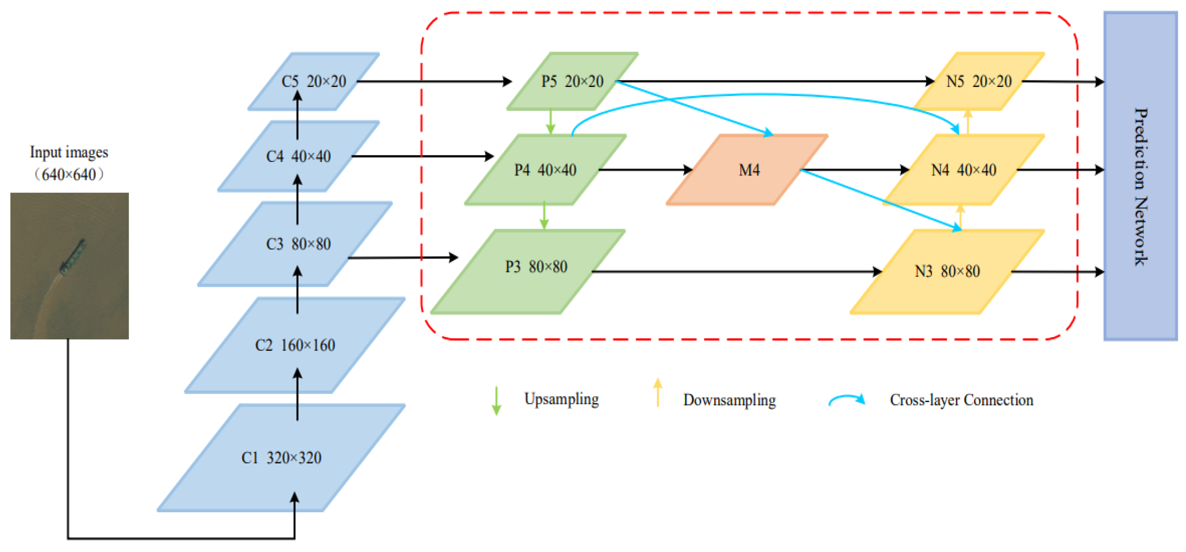
Figure 4.
BiFPN feature fusion network.
Figure 4.
BiFPN feature fusion network.
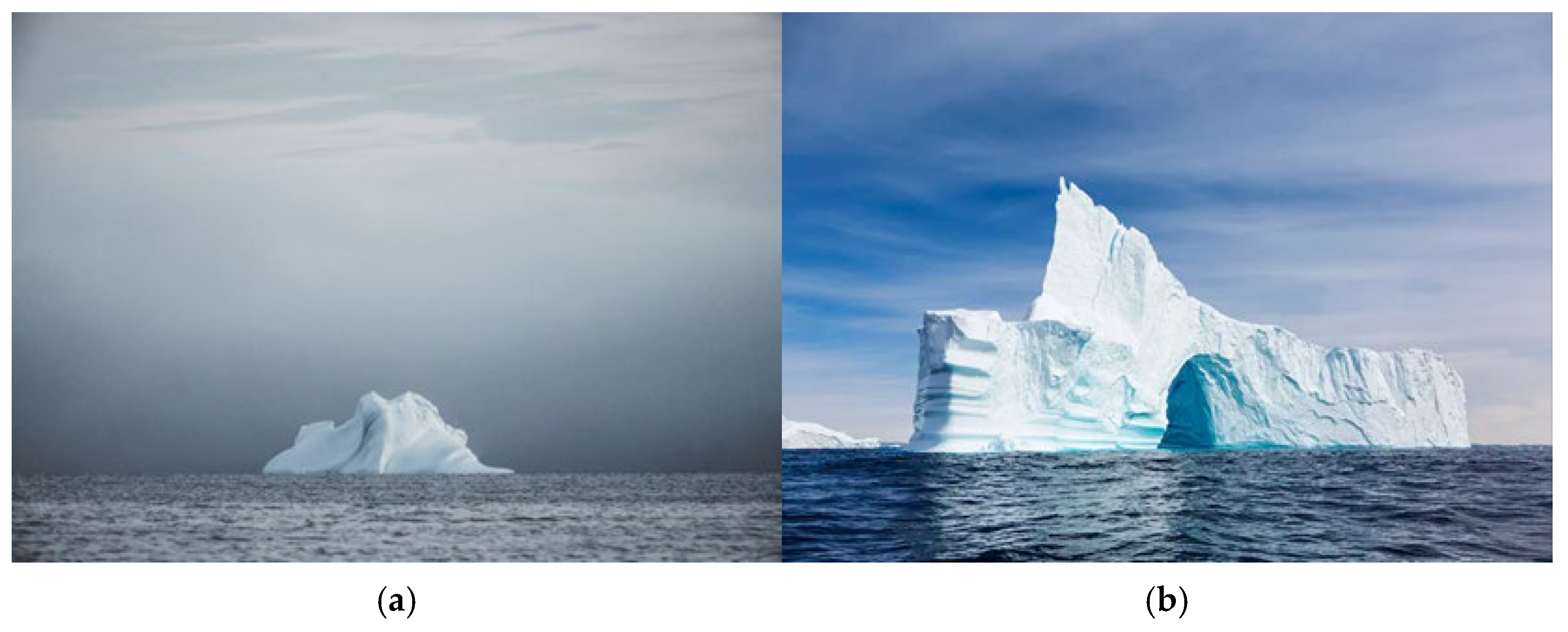
Figure 5.
Dataset collection examples for polar environmental target detection: (
a,
b) images collected from
https://m.51miz.com/so-tupian/7413673.html (accessed on 13 October 2025); (
c,
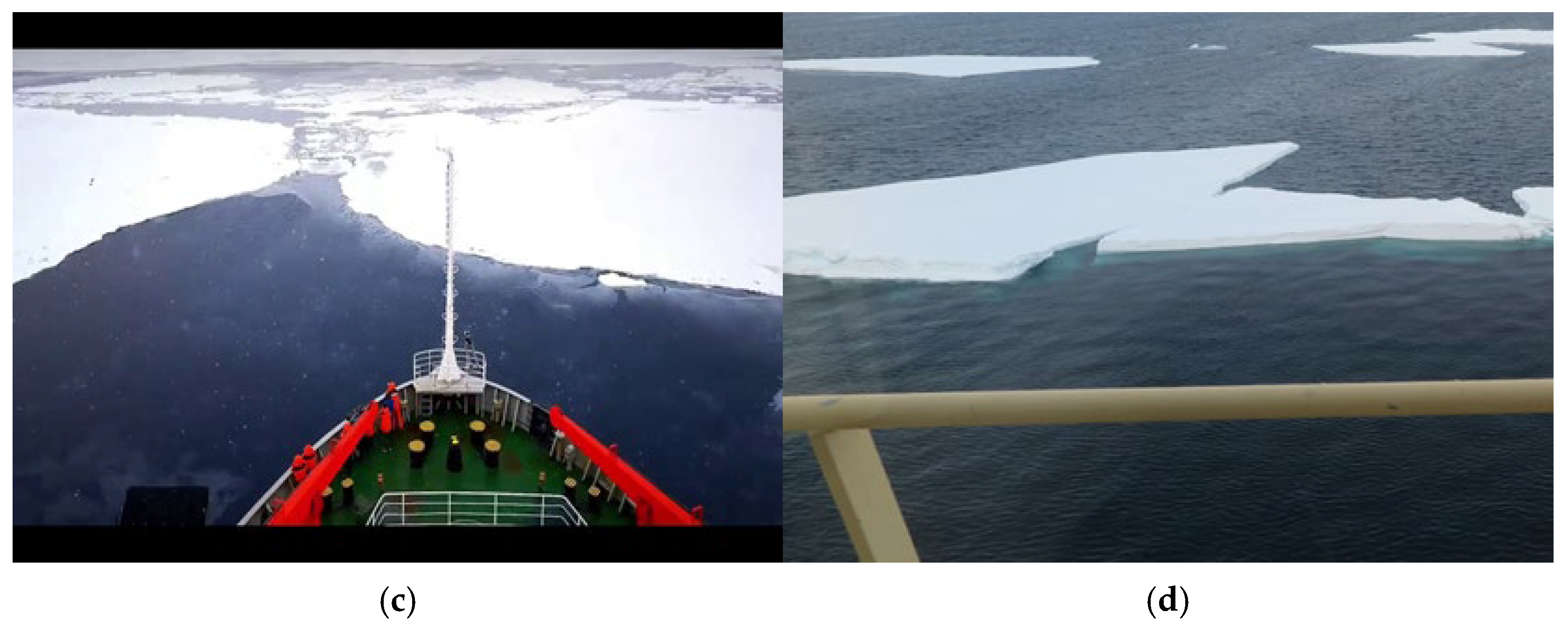
d) frames extracted from polar videos.
Figure 5.
Dataset collection examples for polar environmental target detection: (
a,
b) images collected from
https://m.51miz.com/so-tupian/7413673.html (accessed on 13 October 2025); (
c,
d) frames extracted from polar videos.
Figure 6.
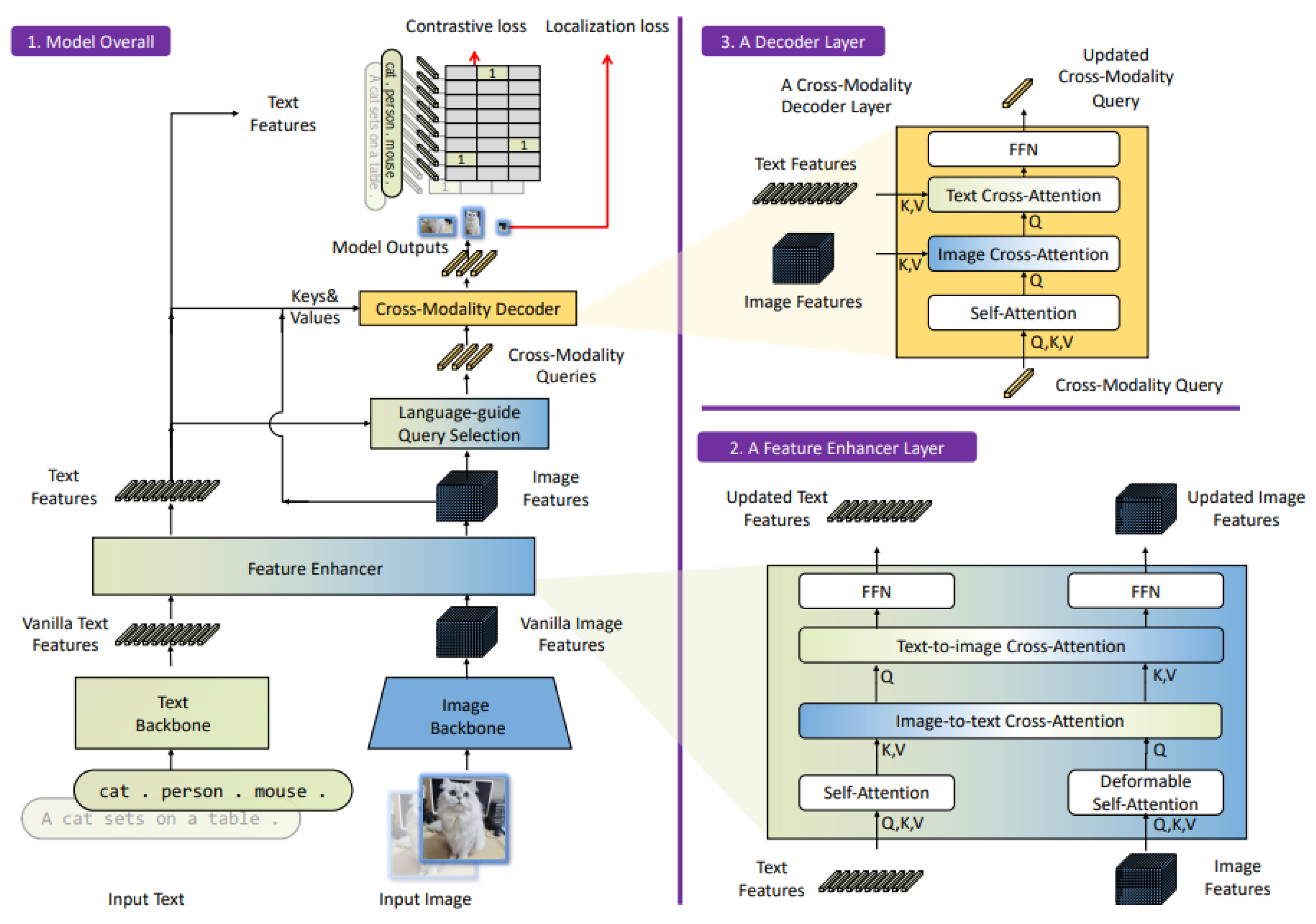
Principle diagram of Grounding DINO.
Figure 6.
Principle diagram of Grounding DINO.
Figure 7.
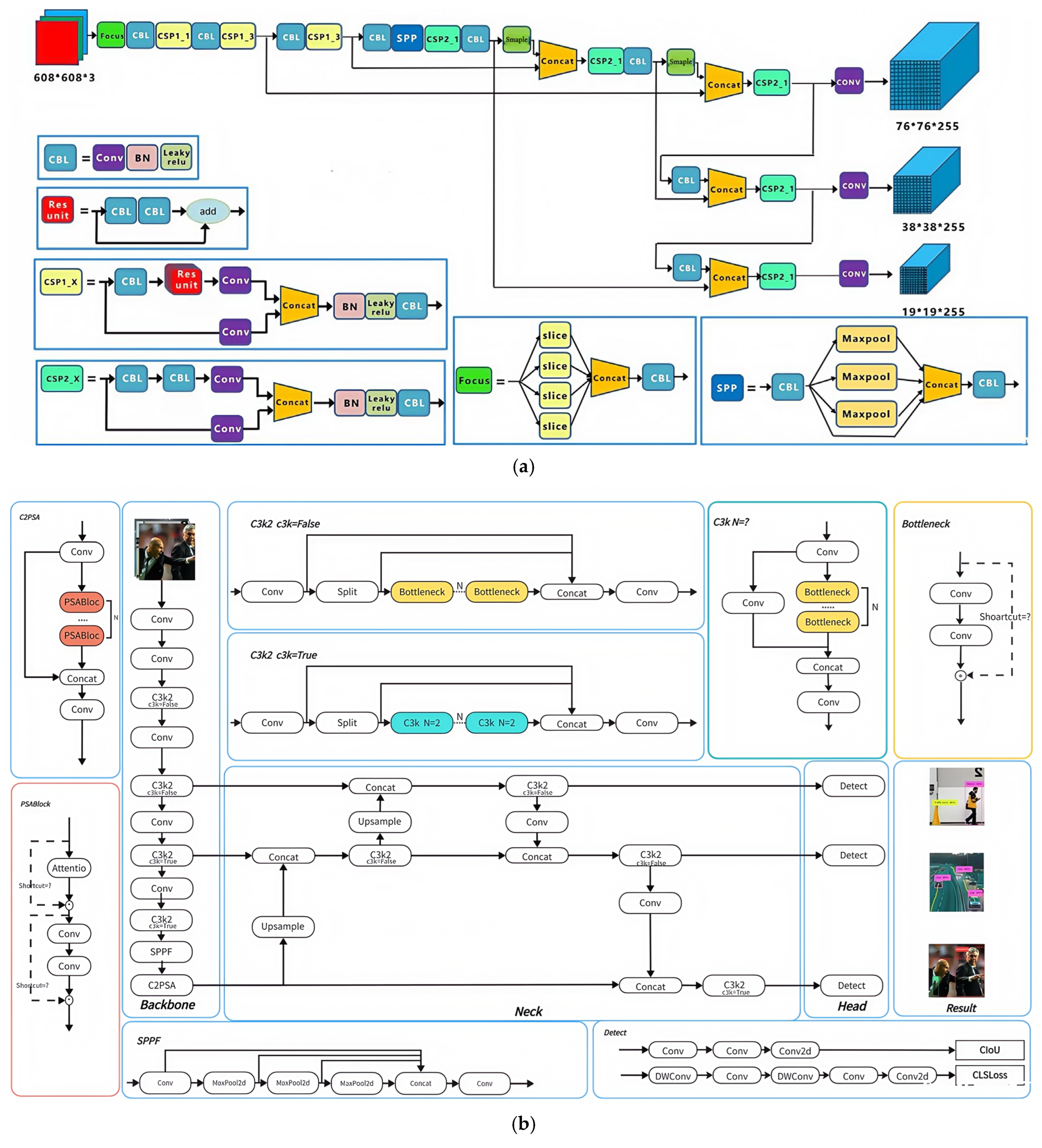
Network architecture comparison of (a) YOLOv5n and (b) YOLOv11n.
Figure 7.
Network architecture comparison of (a) YOLOv5n and (b) YOLOv11n.
Figure 8.
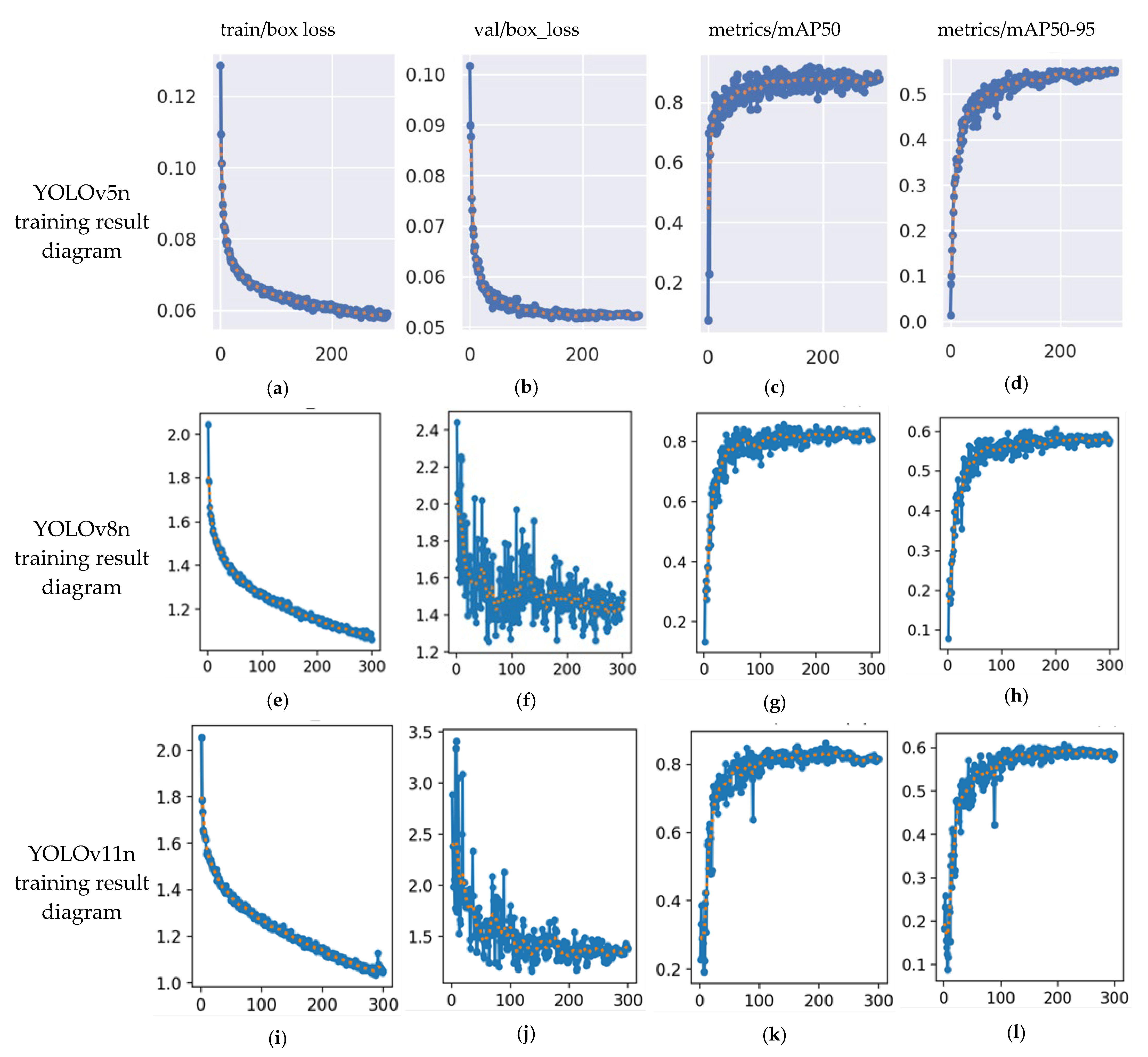
Training result diagrams of YOLOv5n (a–d), YOLOv8n (e–h), and YOLOv11n (i–l), where blue lines indicate raw values per iteration, and orange dots show smoothed trends to highlight convergence.
Figure 8.
Training result diagrams of YOLOv5n (a–d), YOLOv8n (e–h), and YOLOv11n (i–l), where blue lines indicate raw values per iteration, and orange dots show smoothed trends to highlight convergence.
Figure 9.
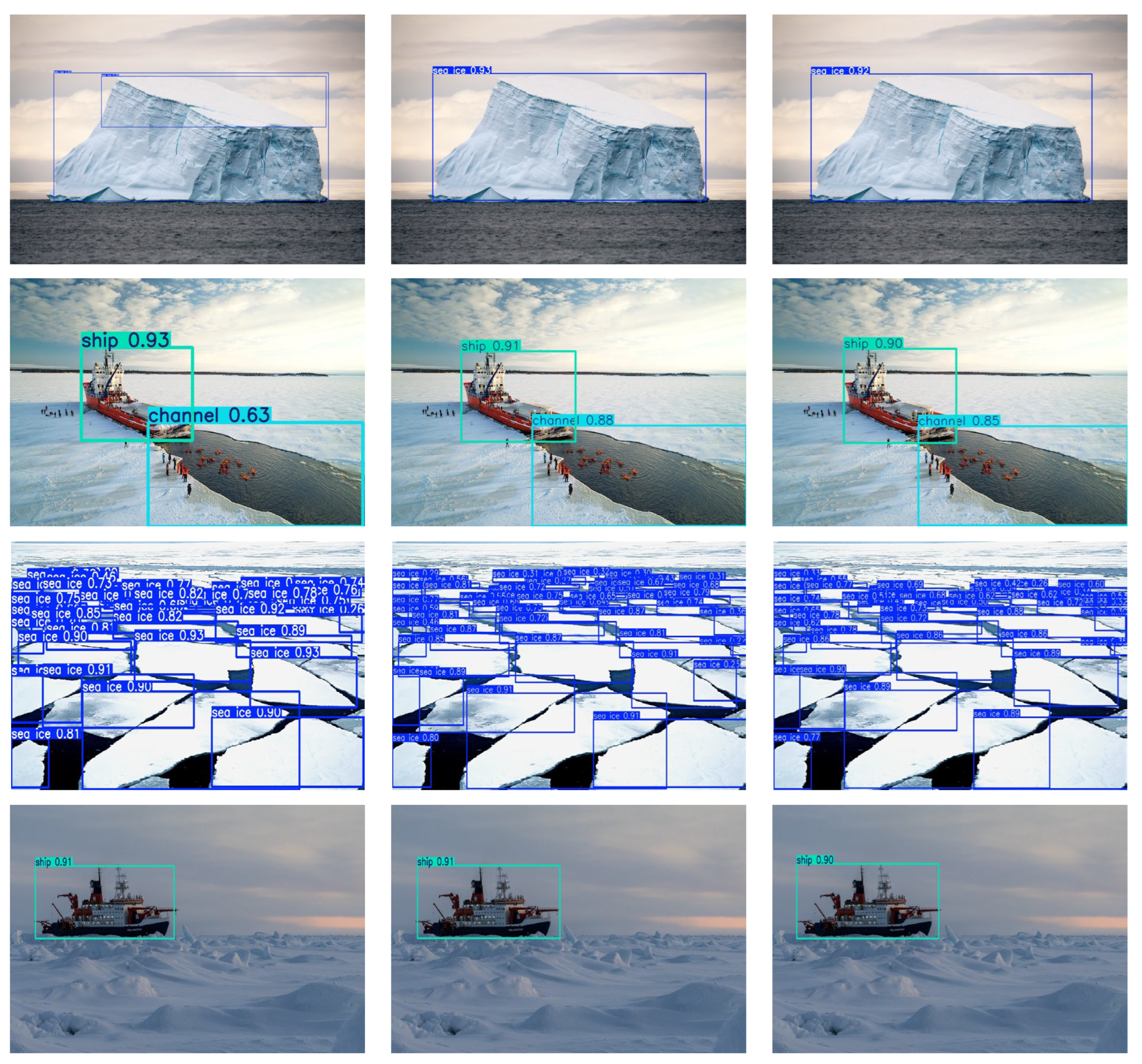
Comparison of data test results for polar targets using different versions of YOLO. From left to right, YOLOv5n, YOLOv8n, and YOLOv11n, and from top to bottom, icebergs, ships and channels, sea ice, and ships.
Figure 9.
Comparison of data test results for polar targets using different versions of YOLO. From left to right, YOLOv5n, YOLOv8n, and YOLOv11n, and from top to bottom, icebergs, ships and channels, sea ice, and ships.
Figure 10.
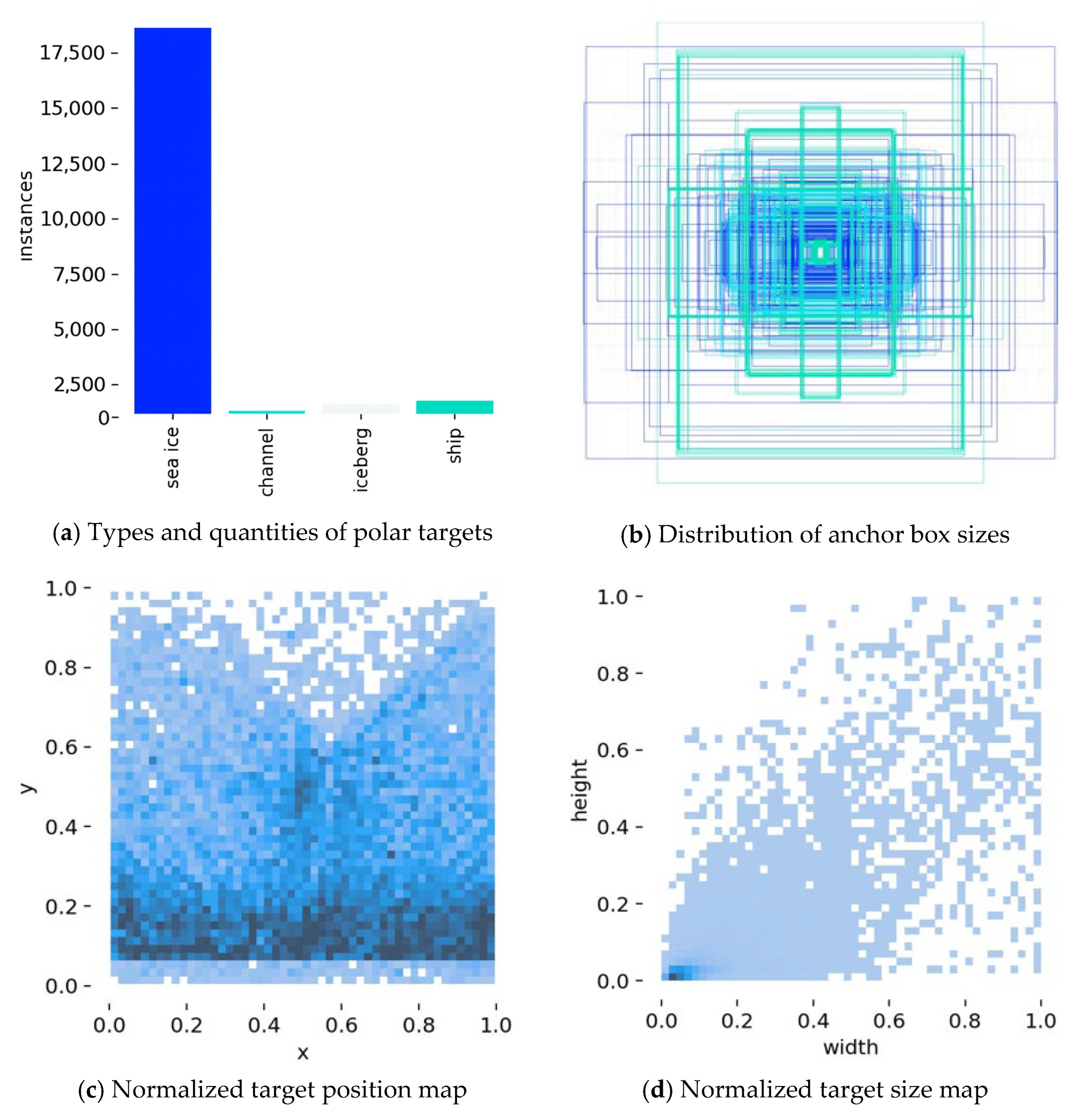
Polar targets data distribution diagram, where different colors indicate different target types.
Figure 10.
Polar targets data distribution diagram, where different colors indicate different target types.
Figure 11.
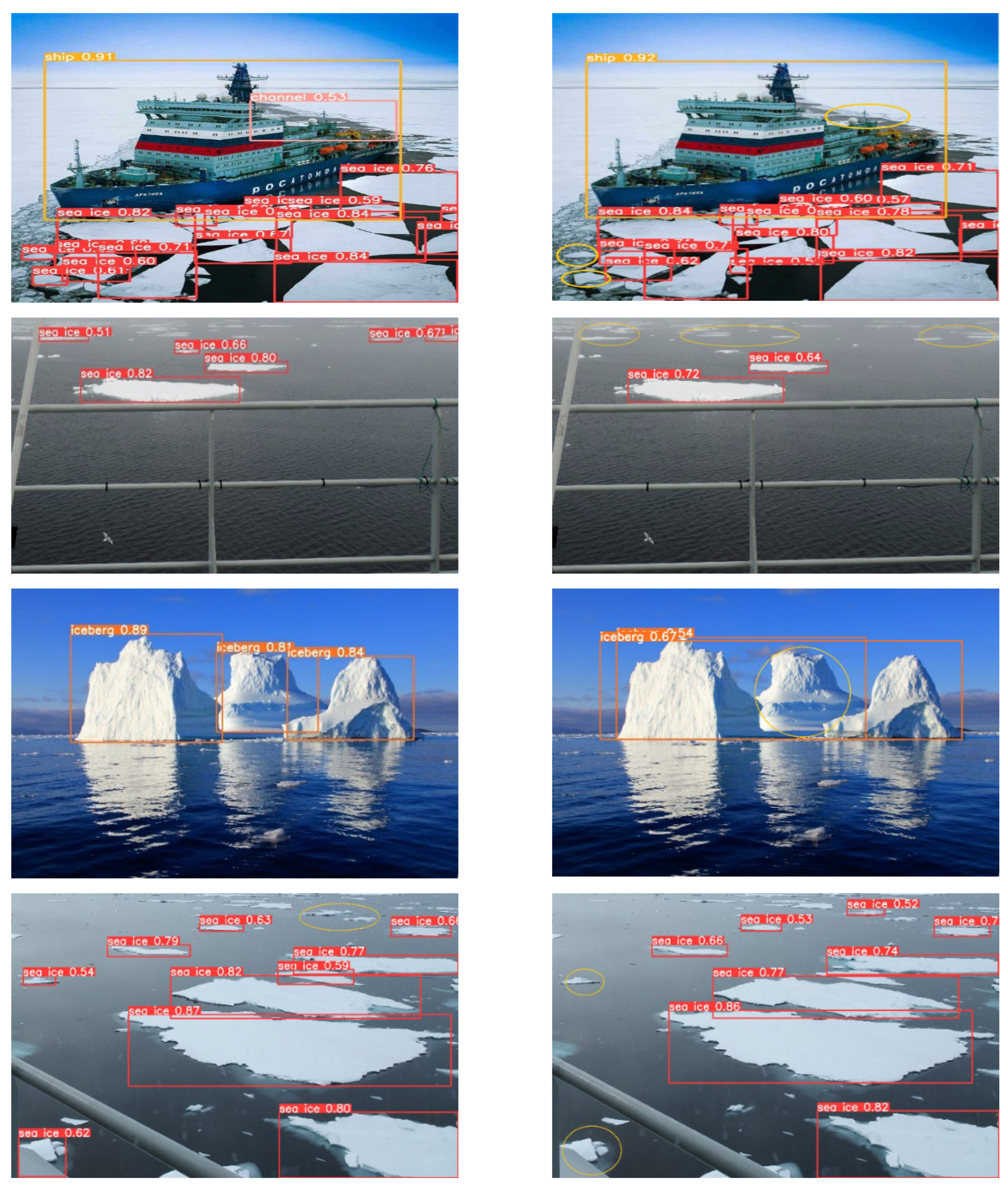
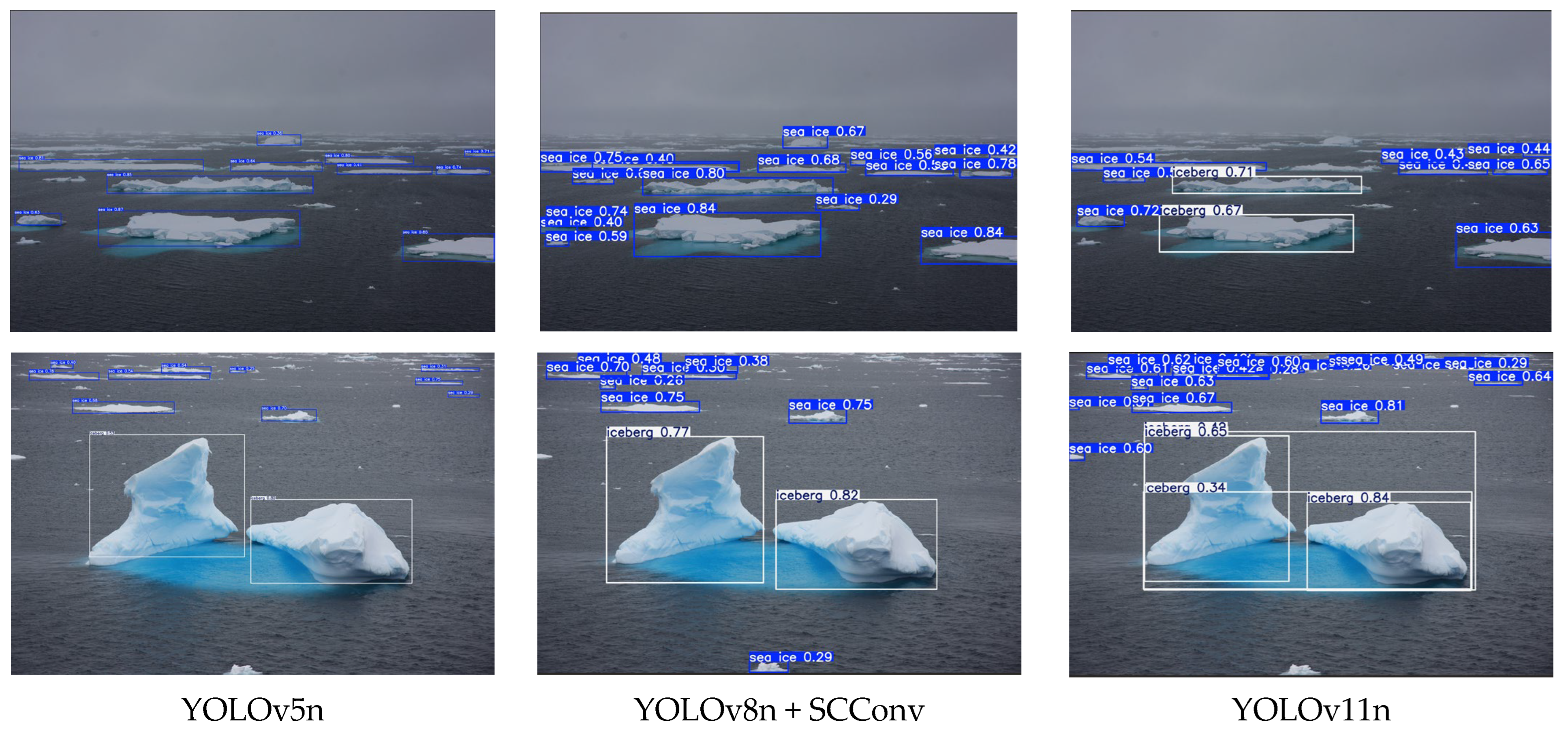
Comparison visualization of YOLOv8n+ SCConv and YOLOv8n, from left to right, and YOLOv8n + SCConv and YOLOv8n, from top to bottom, are ships and ice channel, ships and sea ice, sea ice, icebergs, and sea ice.
Figure 11.
Comparison visualization of YOLOv8n+ SCConv and YOLOv8n, from left to right, and YOLOv8n + SCConv and YOLOv8n, from top to bottom, are ships and ice channel, ships and sea ice, sea ice, icebergs, and sea ice.
Figure 12.
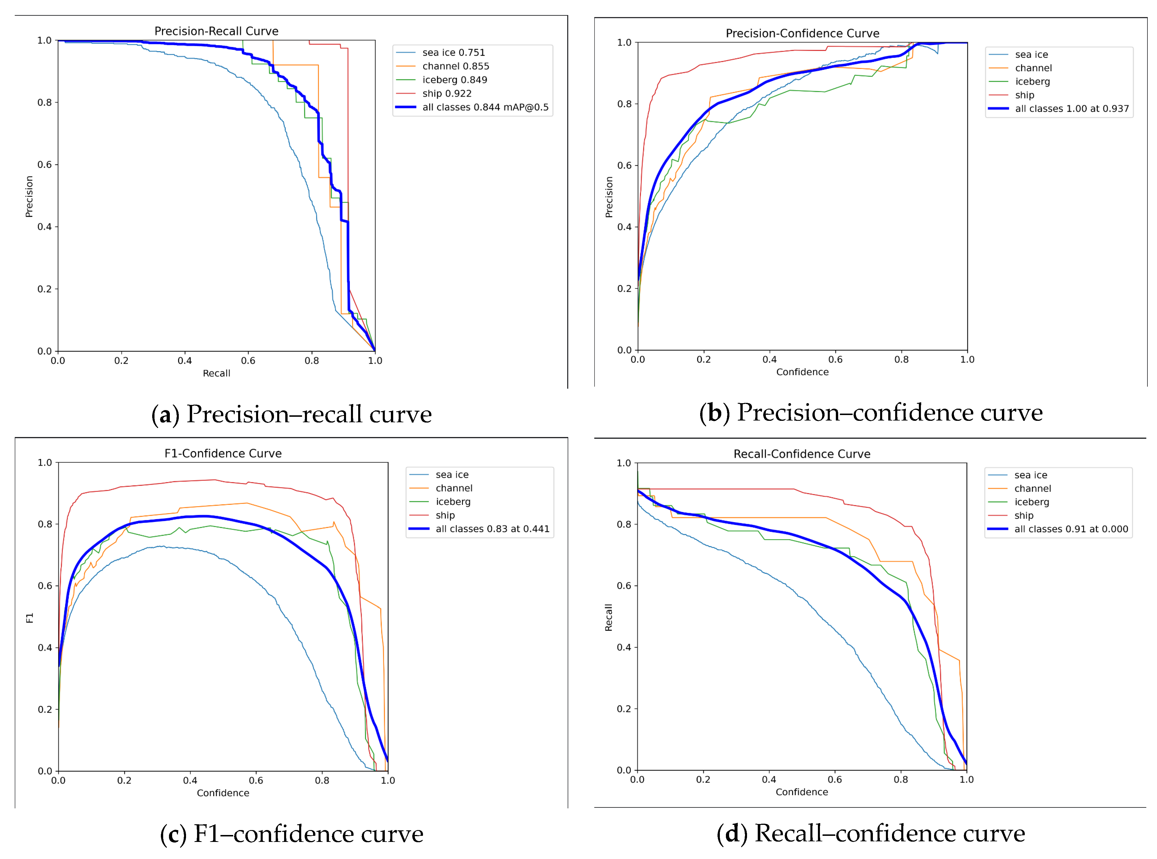
Training process visualization.
Figure 12.
Training process visualization.
Figure 13.
YOLOv8n training results diagram.
Figure 13.
YOLOv8n training results diagram.
Figure 14.
YOLOv8n training results based on SCConv.
Figure 14.
YOLOv8n training results based on SCConv.
Figure 15.
YOLOv8n training results with BiFPN network integration.
Figure 15.
YOLOv8n training results with BiFPN network integration.
Figure 16.
Image recognition results interface.
Figure 16.
Image recognition results interface.
Figure 17.
Image recognition result interface, from top to bottom, are the channel and ship, sea ice, and icebergs, and from left to right, YOLOv5n, YOLOv8n, and YOLOv11n.
Figure 17.
Image recognition result interface, from top to bottom, are the channel and ship, sea ice, and icebergs, and from left to right, YOLOv5n, YOLOv8n, and YOLOv11n.
Figure 18.
Polar environment target recognition map generated by stable diffusion.
Figure 18.
Polar environment target recognition map generated by stable diffusion.
Figure 19.
Confusion matrix comparison of YOLOv5n, YOLOv8n, and YOLOv11n for classification performance.
Figure 19.
Confusion matrix comparison of YOLOv5n, YOLOv8n, and YOLOv11n for classification performance.
Table 1.
Comparison table with Faster R-CNN, SSD, and RetinaNet.
Table 1.
Comparison table with Faster R-CNN, SSD, and RetinaNet.
| Index | YOLOv8n | Faster R-CNN | RetinaNet | SSD |
|---|
| Detection speed | Faster | Slower | Slower | Slightly slower |
| Detection accuracy | Slightly lower | Higher | Higher | Higher |
| Memory occupation | Smaller | Larger | Larger | Larger |
Table 2.
Distribution of images by target labels in the polar targets dataset.
Table 2.
Distribution of images by target labels in the polar targets dataset.
| Label Name | Iceberg | Sea Ice | Ice Channel | Ship | Total |
|---|
| Number of images | 354 | 588 | 261 | 439 | 1342 |
| Images collected from websites | 263 | 438 | 194 | 327 | 998 |
| Frames extracted from polar videos | 91 | 150 | 67 | 112 | 344 |
Table 3.
Pseudocode for data pre-annotation strategy based on Grounding DINO.
Table 3.
Pseudocode for data pre-annotation strategy based on Grounding DINO.
| Pre-Annotation Pseudocode |
|---|
| Load Grounding DINO model with pretrained weights |
| image_dataset = LoadPEGData() |
| text_prompt = “iceberg, sea ice, channel, ship” |
| for each image in image_dataset: |
| image_features = VisualEncoder(image) |
| text_features = TextEncoder(text_prompt) |
| fused_features = FeatureEnhancer (image_features, text_features) |
| queries = LanguageGuidedQuerySelector (fused_features, text_features) |
| bboxes = CrossModalityDecoder(queries) |
| annotated_image = DrawBBoxes (image, bboxes, text_prompt) |
| SaveAnnotatedData(annotated_image) |
Table 4.
Comparison of different versions of YOLO.
Table 4.
Comparison of different versions of YOLO.
| Experiment | Detection Model | mAP | P | R | F1 | Single-Image Detection Time (ms) | Weight (MB) |
|---|
| 1 | YOLOv5n | 0.825 | 0.951 | 0.870 | 0.810 | 13.3 | 3.9 |
| 2 | YOLOv8n | 0.830 | 0.957 | 0.880 | 0.830 | 6.8 | 6.2 |
| 3 | YOLOv11n | 0.815 | 0.969 | 0.870 | 0.810 | 9.2 | 5.4 |
Table 5.
Comparison of training results for improved YOLOv8n (highest value bolded).
Table 5.
Comparison of training results for improved YOLOv8n (highest value bolded).
| Experiment | Detection Model | mAP | P | R | F1 | Single-Image Detection Time (ms) | Weight (MB) |
|---|
| 1 | YOLOv8n | 0.830 | 0.957 | 0.88 | 0.83 | 6.8 | 6.2 |
| 2 | YOLOv8n + SE | 0.810 | 0.933 | 0.88 | 0.79 | 7.0 | 12.2 |
| 3 | YOLOv8n + CBAM | 0.803 | 0.889 | 0.88 | 0.79 | 8.0 | 12.2 |
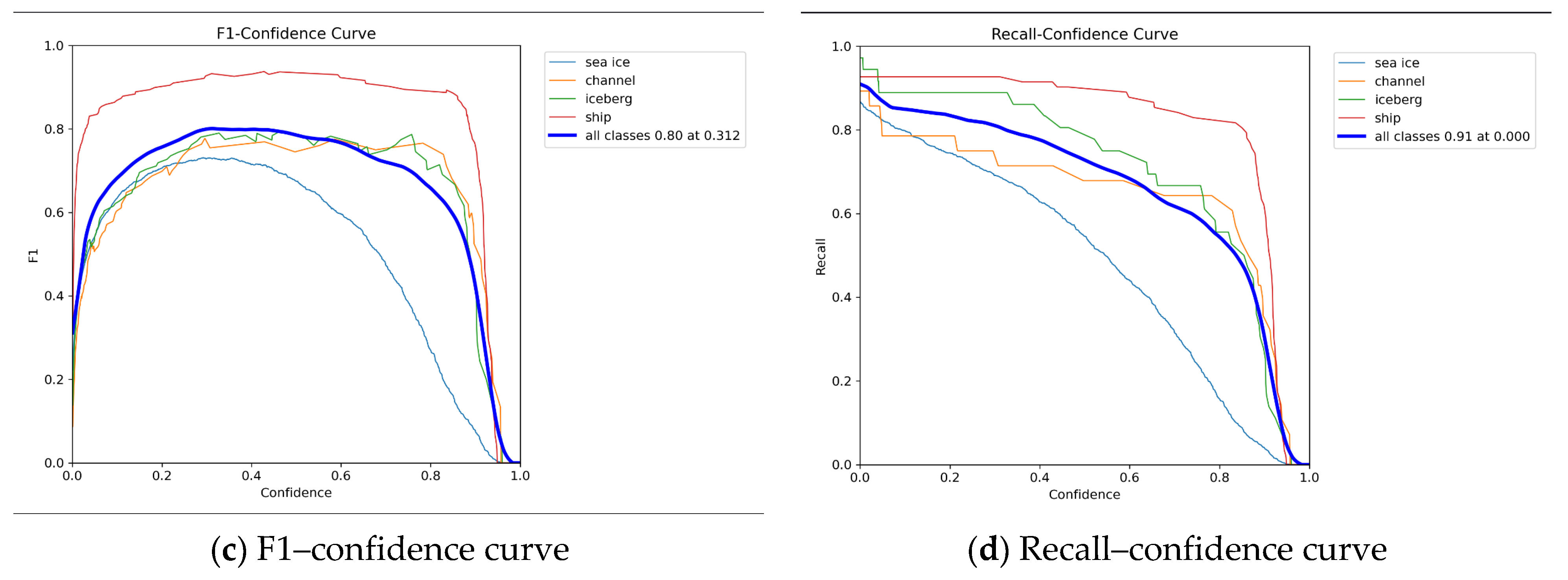
| 4 | YOLOv8n + BiFPN | 0.829 | 0.953 | 0.91 | 0.80 | 8.1 | 5.9 |
| 5 | YOLOv8n + SCConv | 0.844 | 0.937 | 0.91 | 0.83 | 6.8 | 6.0 |
| 6 | YOLOv8n + AKConv | 0.814 | 0.928 | 0.89 | 0.78 | 9.2 | 6.2 |
Table 6.
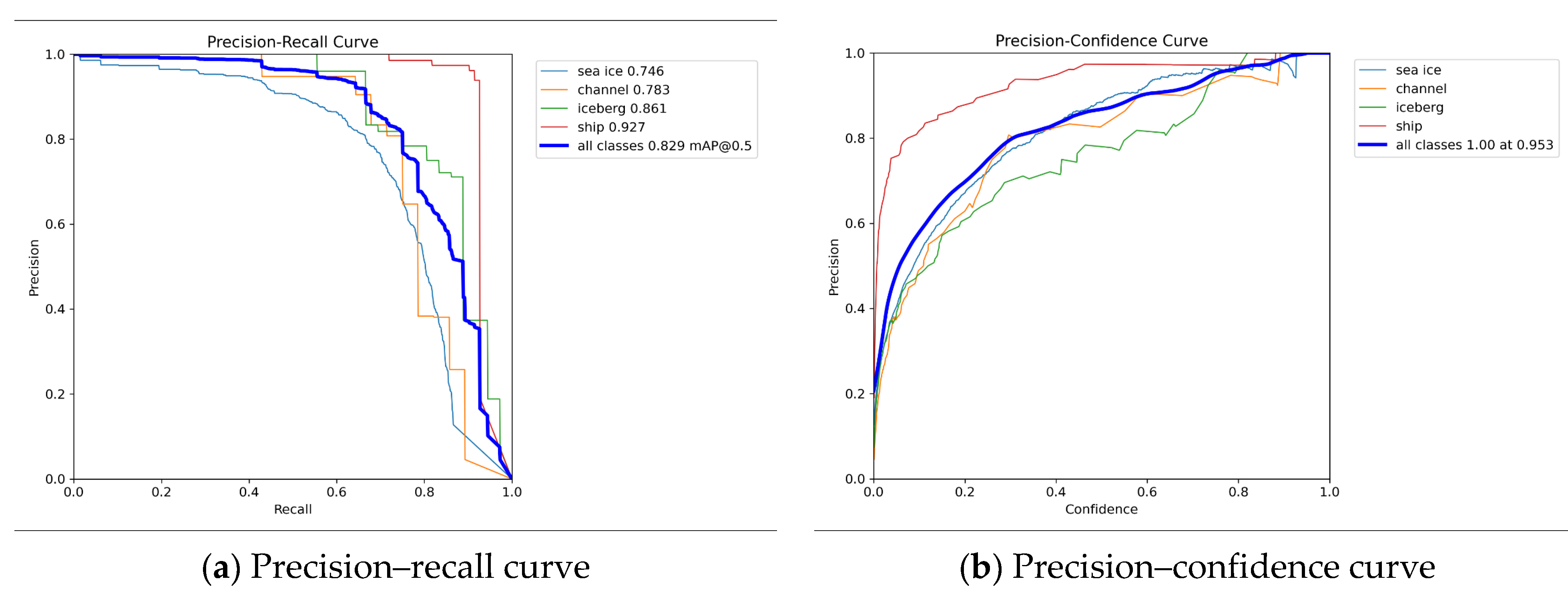
Comparison chart of polar targets data training results (highest value bolded).
Table 6.
Comparison chart of polar targets data training results (highest value bolded).
| Detection Model | Sea Ice | Channel | Iceberg | Ship | mAP@50 |
|---|
| YOLOv8n | 0.736 | 0.843 | 0.802 | 0.942 | 0.830 |
| YOLOv8n + SE | 0.738 | 0.785 | 0.780 | 0.937 | 0.810 |
| YOLOv8n + CBAM | 0.746 | 0.747 | 0.789 | 0.928 | 0.803 |
| YOLOv8n + BiFPN | 0.746 | 0.783 | 0.861 | 0.927 | 0.829 |
| YOLOv8n + SCConv | 0.751 | 0.855 | 0.849 | 0.922 | 0.844 |
| YOLOv8n + AKConv | 0.729 | 0.719 | 0.870 | 0.939 | 0.814 |
Table 7.
Image generation process of stable diffusion based on predefined text prompts.
Table 7.
Image generation process of stable diffusion based on predefined text prompts.
| Image Generation via Text Prompts |
|---|
| “A large iceberg floating in the Arctic Ocean with clear sky.” |
| “Sea ice covering the Antarctic coastline with penguins in the background.” |
| “A polar bear walking on thin sea ice in the Arctic.” |
| “A ship navigating through dense sea ice in the Arctic.” |
| “A group of icebergs in the Arctic with aurora borealis in the sky.” |
| “A close-up view of a melting iceberg in the Arctic.” |
| “A ship stuck in thick sea ice in the Antarctic.” |
| “A wide shot of the Arctic landscape with multiple icebergs and sea ice.” |
| “A ship breaking through sea ice in the Arctic.” |
| “A detailed view of a ship’s hull interacting with sea ice.” |
