Figure 1.
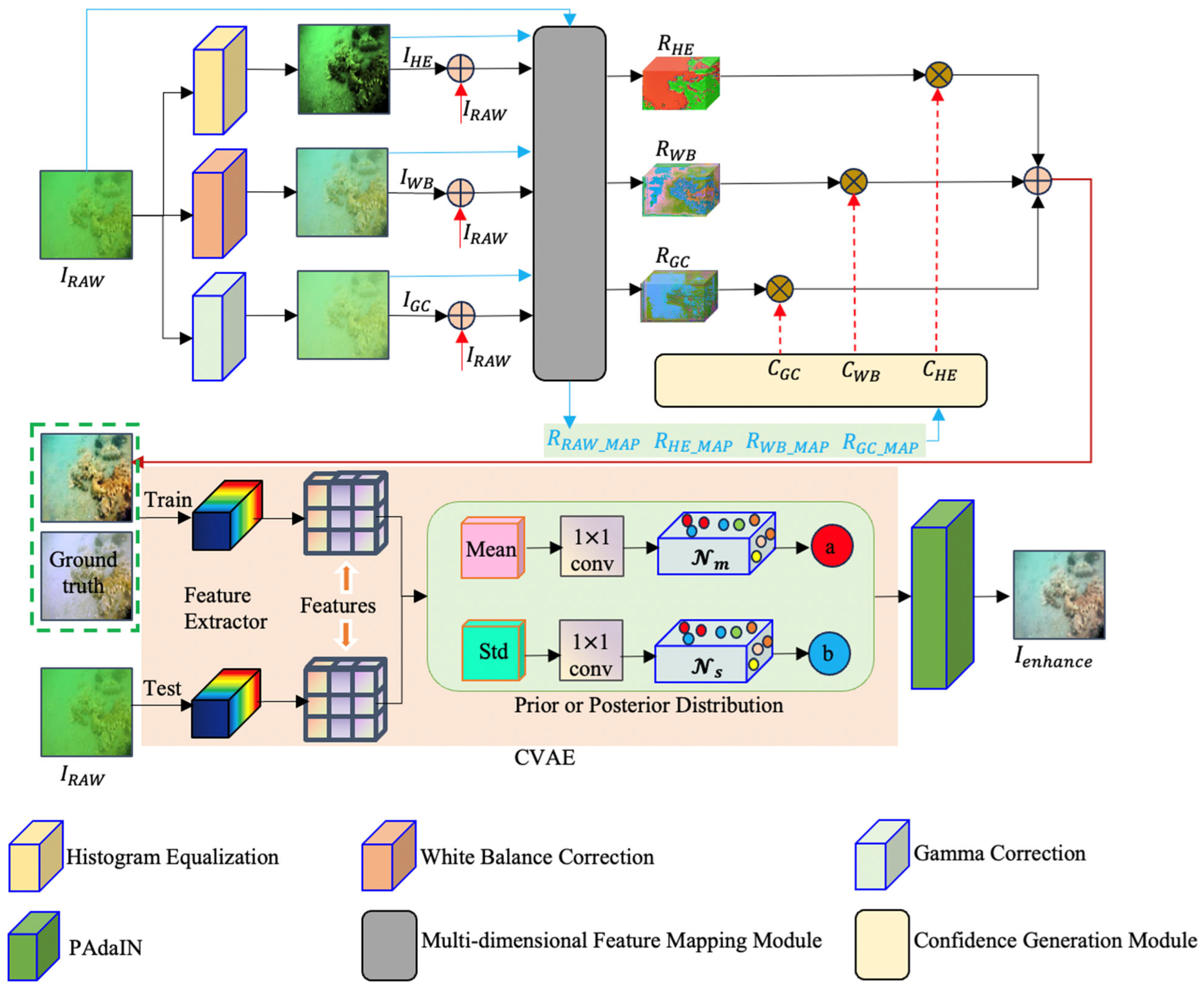
Overall Structure of MFP-PAINet. , , and indicate the feature mappings of , , and , respectively, processed by the multi-dimensional feature mapping module. , , , and indicate the feature mappings of , , , and after processed by the multi-dimensional feature mapping module, which are then inputted into the confidence generation module to generate the confidence maps , , and . indicates the original distorted underwater image; and , , and indicate the results of implementing histogram equalization, white balance correction, and gamma correction to , respectively.
Figure 1.
Overall Structure of MFP-PAINet. , , and indicate the feature mappings of , , and , respectively, processed by the multi-dimensional feature mapping module. , , , and indicate the feature mappings of , , , and after processed by the multi-dimensional feature mapping module, which are then inputted into the confidence generation module to generate the confidence maps , , and . indicates the original distorted underwater image; and , , and indicate the results of implementing histogram equalization, white balance correction, and gamma correction to , respectively.
Figure 2.
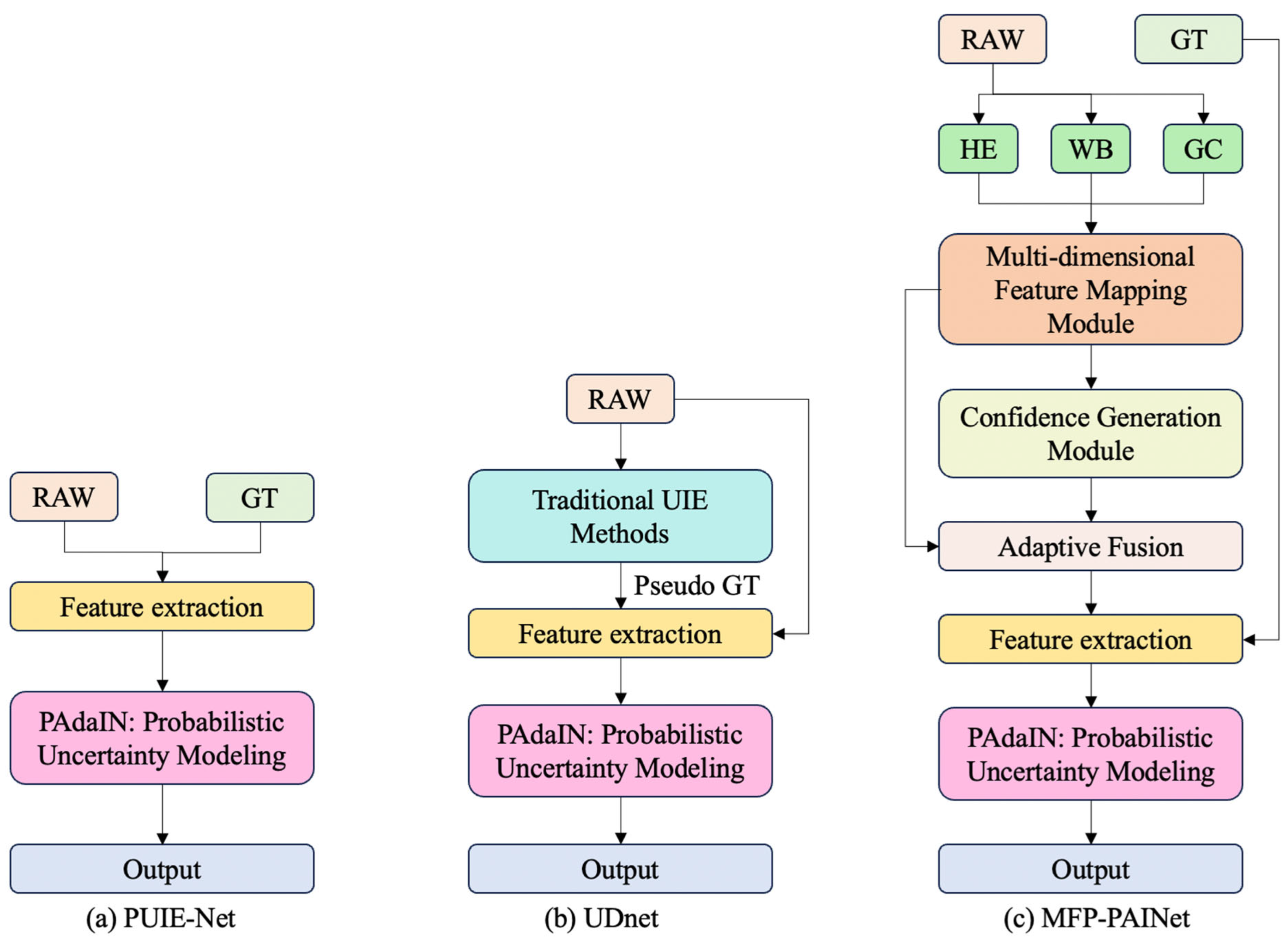
Comparison of the workflow between the proposed MFP-PAINet and existing probabilistic uncertainty modeling methods.
Figure 2.
Comparison of the workflow between the proposed MFP-PAINet and existing probabilistic uncertainty modeling methods.
Figure 3.
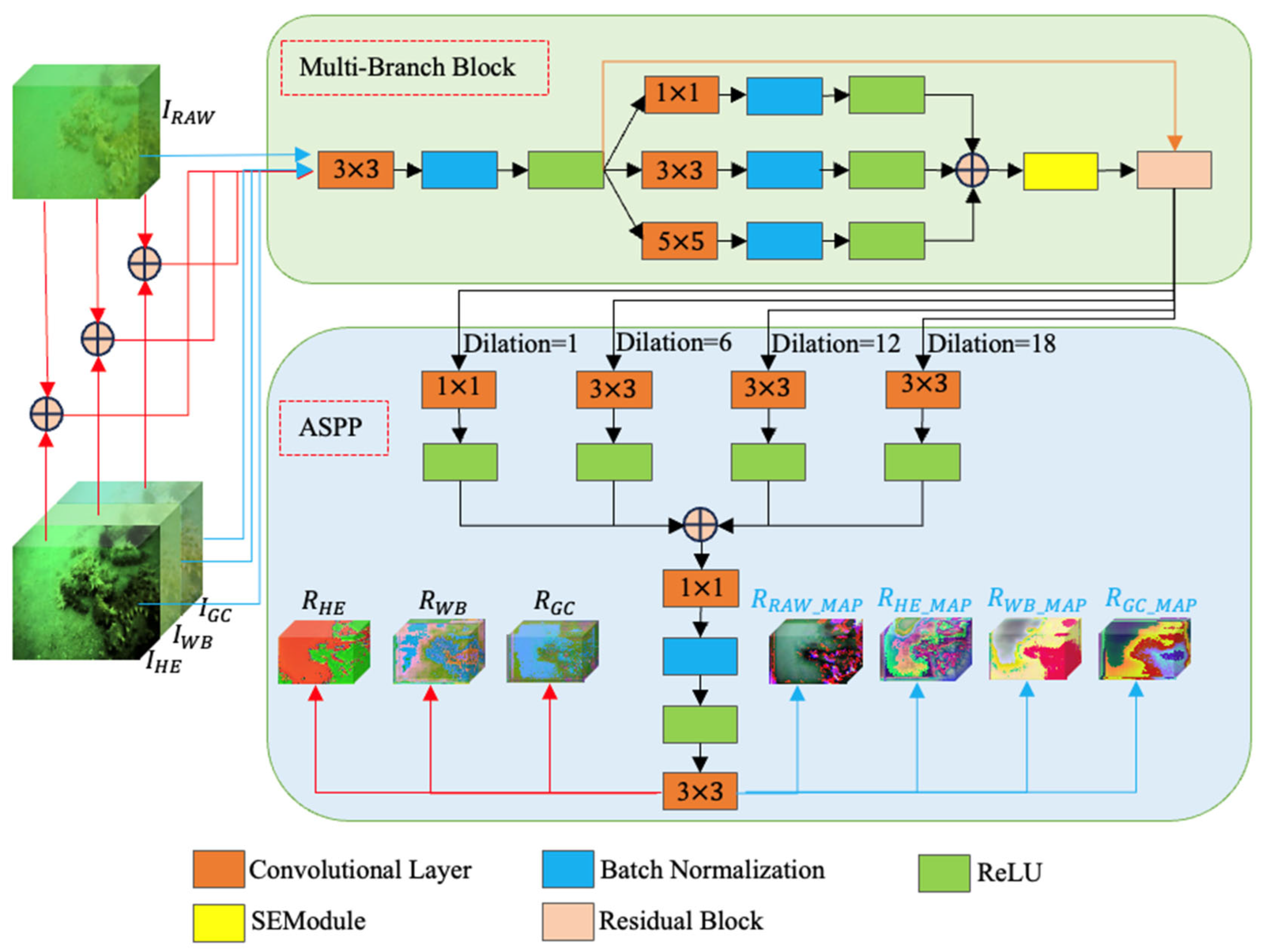
Multi-dimensional Feature Extraction Module. The multi-branch module consists of three branches, each containing 1 1, 3 3, and 5 5 convolutional layers, followed by batch normalization and ReLU activation layers to extract features at different scales. As a commonly used nonlinear activation function, ReLU enhances the network’s nonlinear representation capability and accelerates the model’s convergence. The outputs are finally merged through residual connections. The ASPP module includes 1 1 convolution and several 3 3 convolutional layers with different dilation rates (1, 6, 12, and 18) to capture multi-scale contextual information. The integrated feature maps are further processed through convolution, batch normalization, and ReLU activation layers to ultimately generate multi-dimensional feature representations.
Figure 3.
Multi-dimensional Feature Extraction Module. The multi-branch module consists of three branches, each containing 1 1, 3 3, and 5 5 convolutional layers, followed by batch normalization and ReLU activation layers to extract features at different scales. As a commonly used nonlinear activation function, ReLU enhances the network’s nonlinear representation capability and accelerates the model’s convergence. The outputs are finally merged through residual connections. The ASPP module includes 1 1 convolution and several 3 3 convolutional layers with different dilation rates (1, 6, 12, and 18) to capture multi-scale contextual information. The integrated feature maps are further processed through convolution, batch normalization, and ReLU activation layers to ultimately generate multi-dimensional feature representations.
Figure 4.
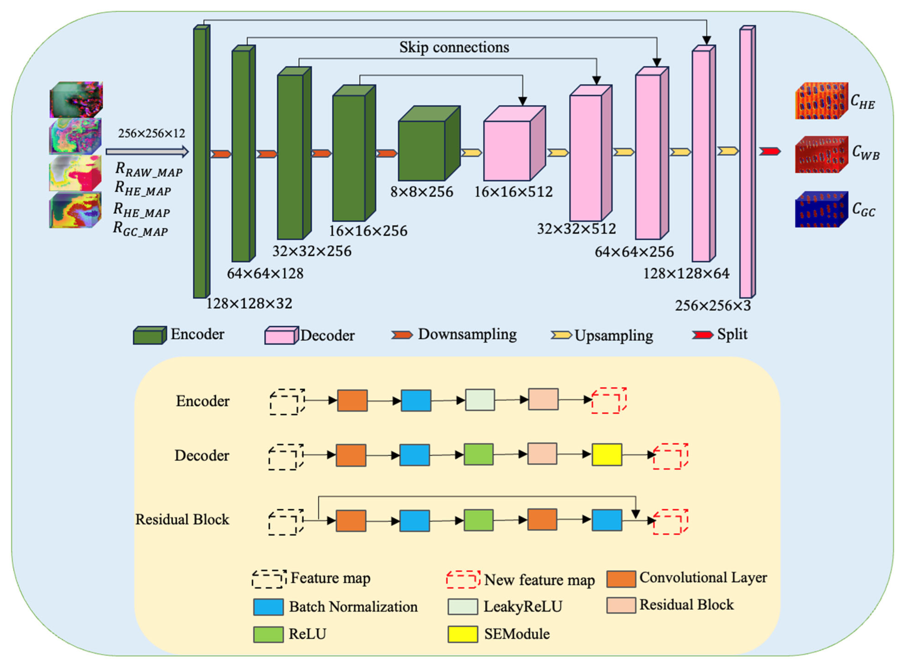
Confidence Generation Network. This module consists of 5 pairs of encoder–decoder structures. Each encoder and decoder includes convolutional layers, batch normalization layers, activation layers and residual blocks to ensure effective feature extraction and representation. In addition, the decoder incorporates an SE attention mechanism to enhance focus on key features. Finally, the Split operation is implemented to process the feature maps within the module, finally acquiring three different confidence maps.
Figure 4.
Confidence Generation Network. This module consists of 5 pairs of encoder–decoder structures. Each encoder and decoder includes convolutional layers, batch normalization layers, activation layers and residual blocks to ensure effective feature extraction and representation. In addition, the decoder incorporates an SE attention mechanism to enhance focus on key features. Finally, the Split operation is implemented to process the feature maps within the module, finally acquiring three different confidence maps.
Figure 5.
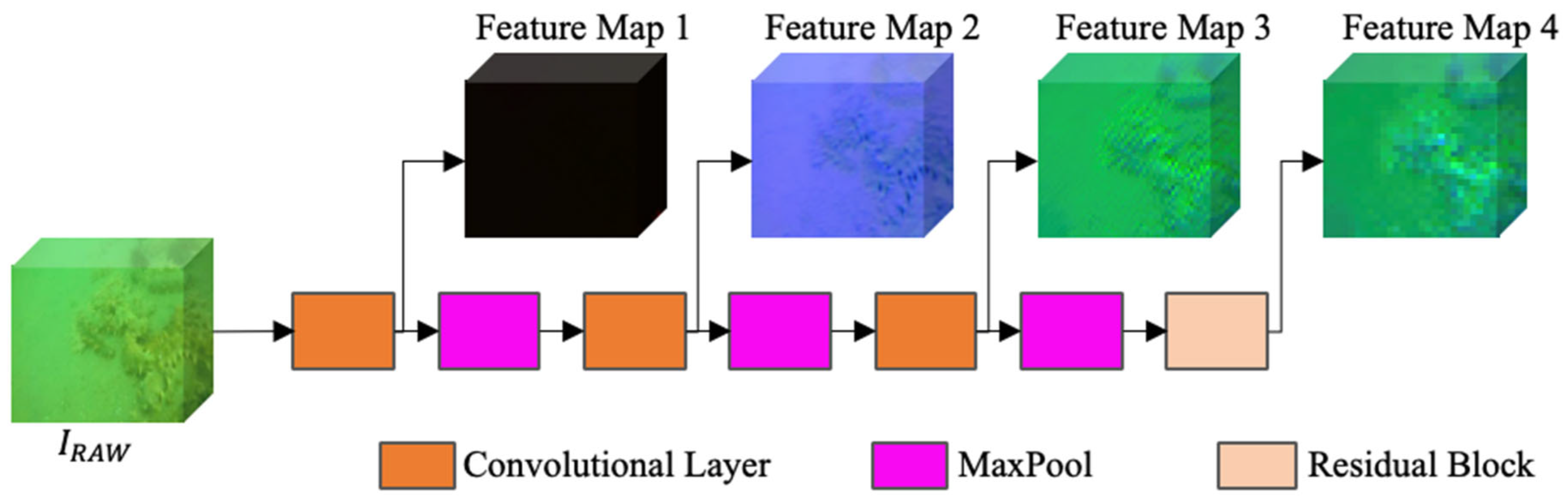
The feature extractor consists of convolutional layers, pooling layers, and residual blocks. It can extract four different scales of feature maps as input for constructing the probability distribution.
Figure 5.
The feature extractor consists of convolutional layers, pooling layers, and residual blocks. It can extract four different scales of feature maps as input for constructing the probability distribution.
Figure 6.
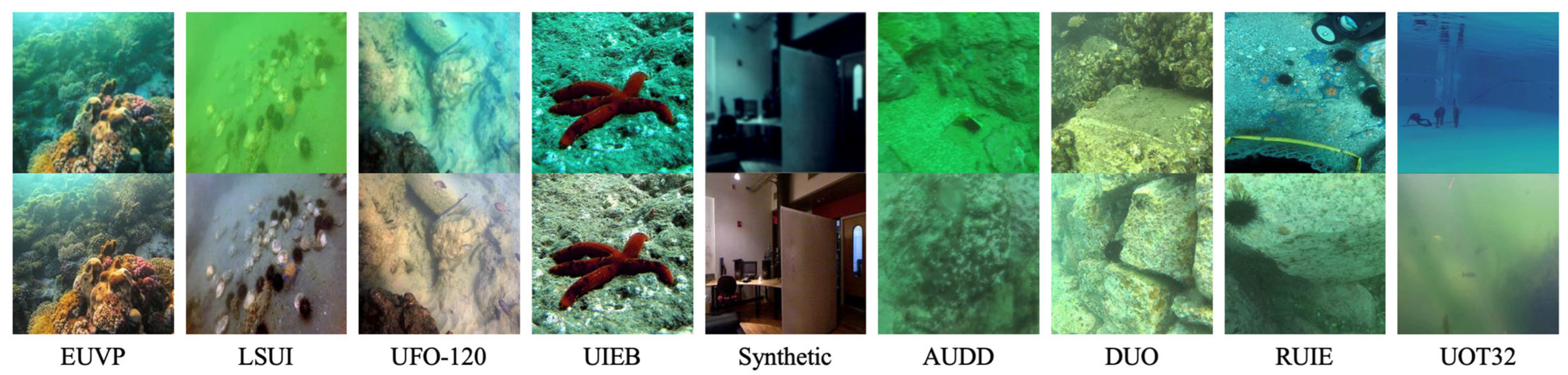
Example images abstracted from each dataset. The first row shows the degraded images, and the second the corresponding reference ones (Note: no reference images are available for RUIE, AUDD, DUO, and UOT32).
Figure 6.
Example images abstracted from each dataset. The first row shows the degraded images, and the second the corresponding reference ones (Note: no reference images are available for RUIE, AUDD, DUO, and UOT32).
Figure 7.
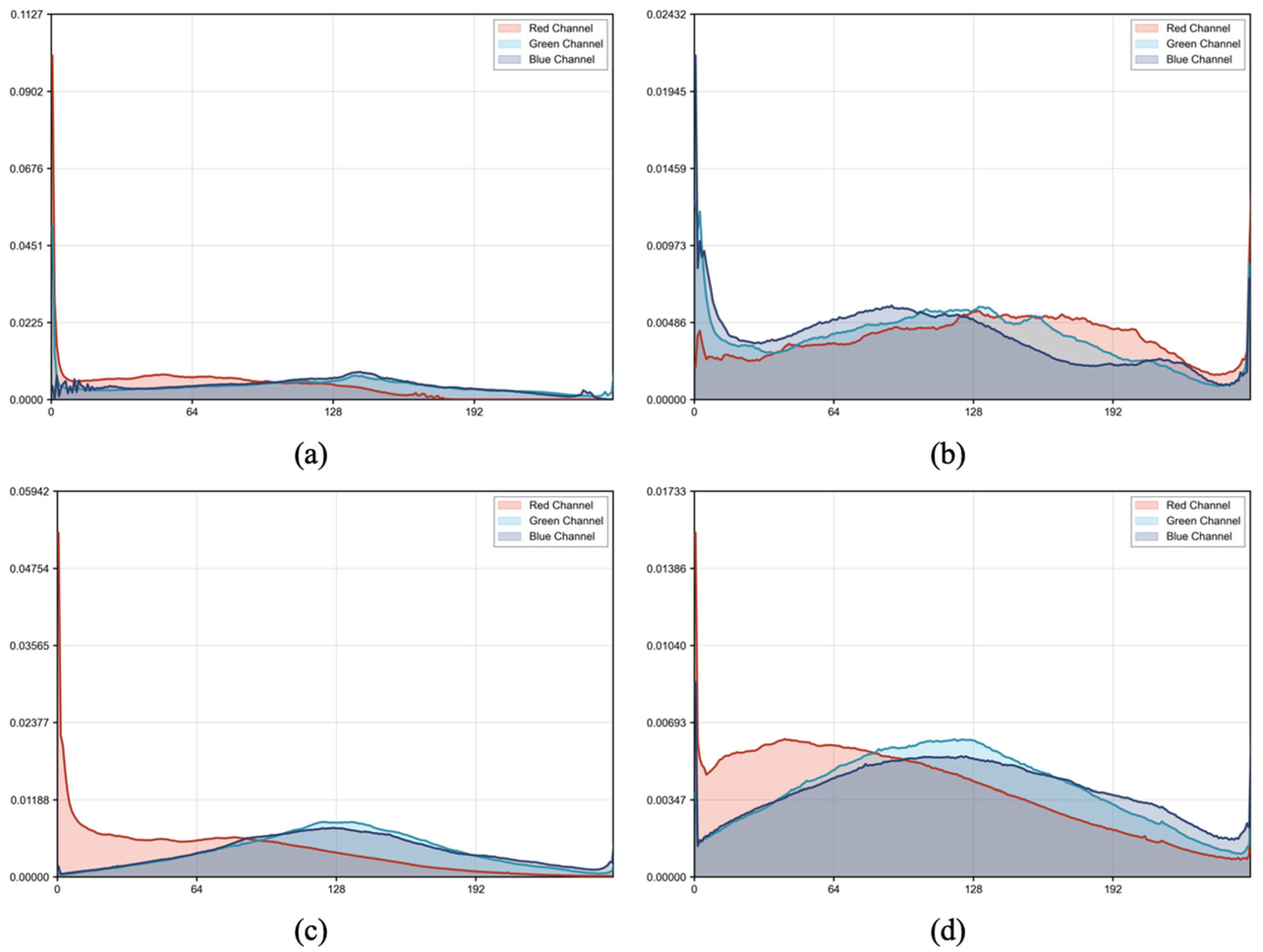
Average RGB distribution statistics on the training datasets: (a,b) represent the synthetic dataset’s distorted images and corresponding ground-truth images, respectively; and (c,d) represent the UIEB dataset’s distorted images and ground-truth images, respectively.
Figure 7.
Average RGB distribution statistics on the training datasets: (a,b) represent the synthetic dataset’s distorted images and corresponding ground-truth images, respectively; and (c,d) represent the UIEB dataset’s distorted images and ground-truth images, respectively.
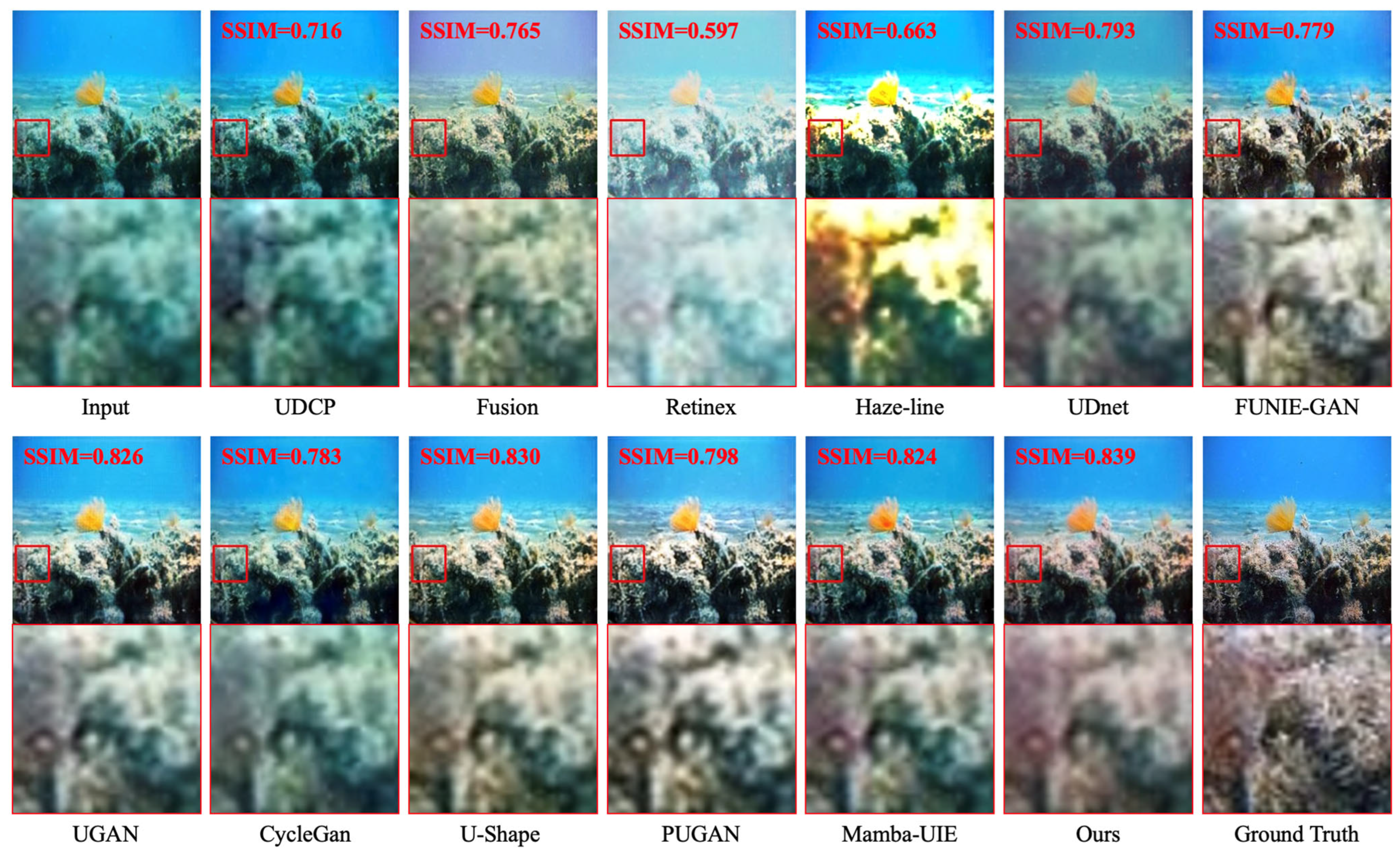
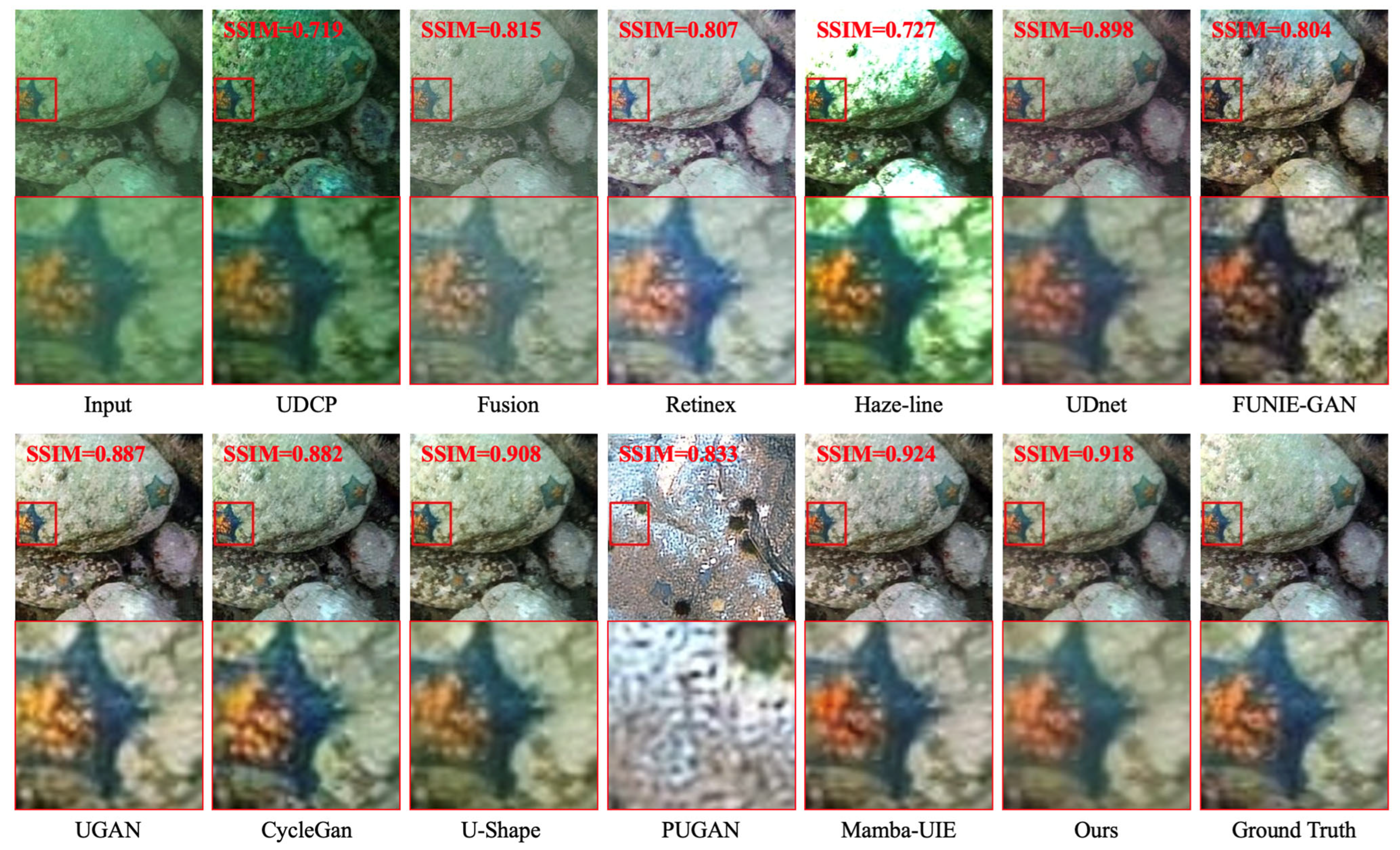
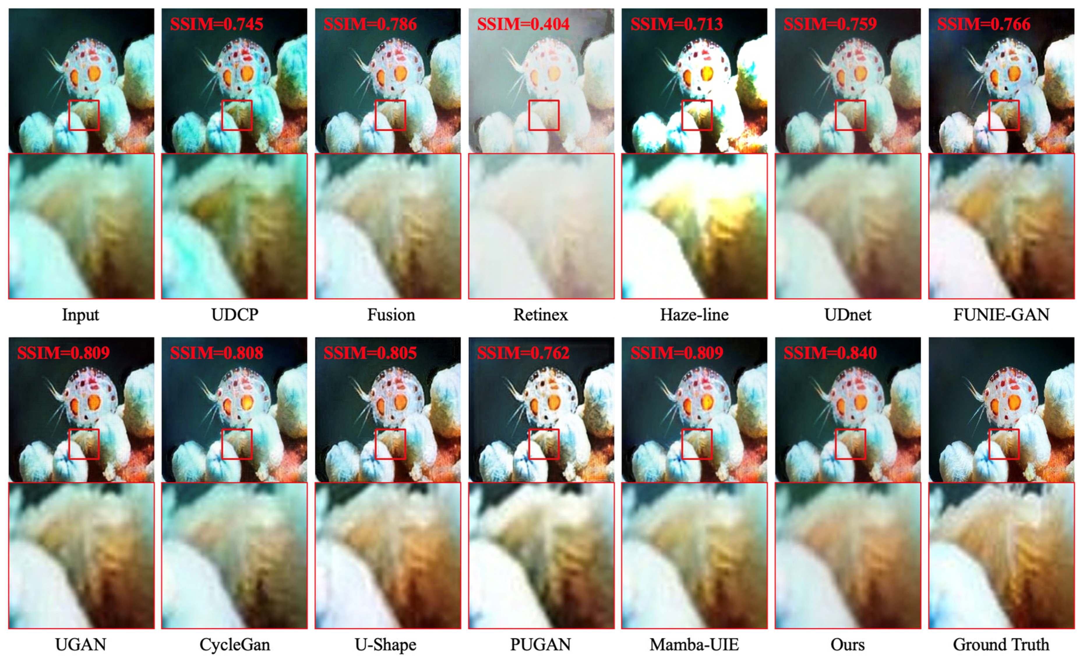
Figure 8.
Enhancement results on the EUVP dataset.
Figure 8.
Enhancement results on the EUVP dataset.
Figure 9.
Enhancement results on the LSUI dataset.
Figure 9.
Enhancement results on the LSUI dataset.
Figure 10.
Enhancement results on the UFO-120 dataset.
Figure 10.
Enhancement results on the UFO-120 dataset.
Figure 11.
Enhancement results on the UIEB dataset.
Figure 11.
Enhancement results on the UIEB dataset.
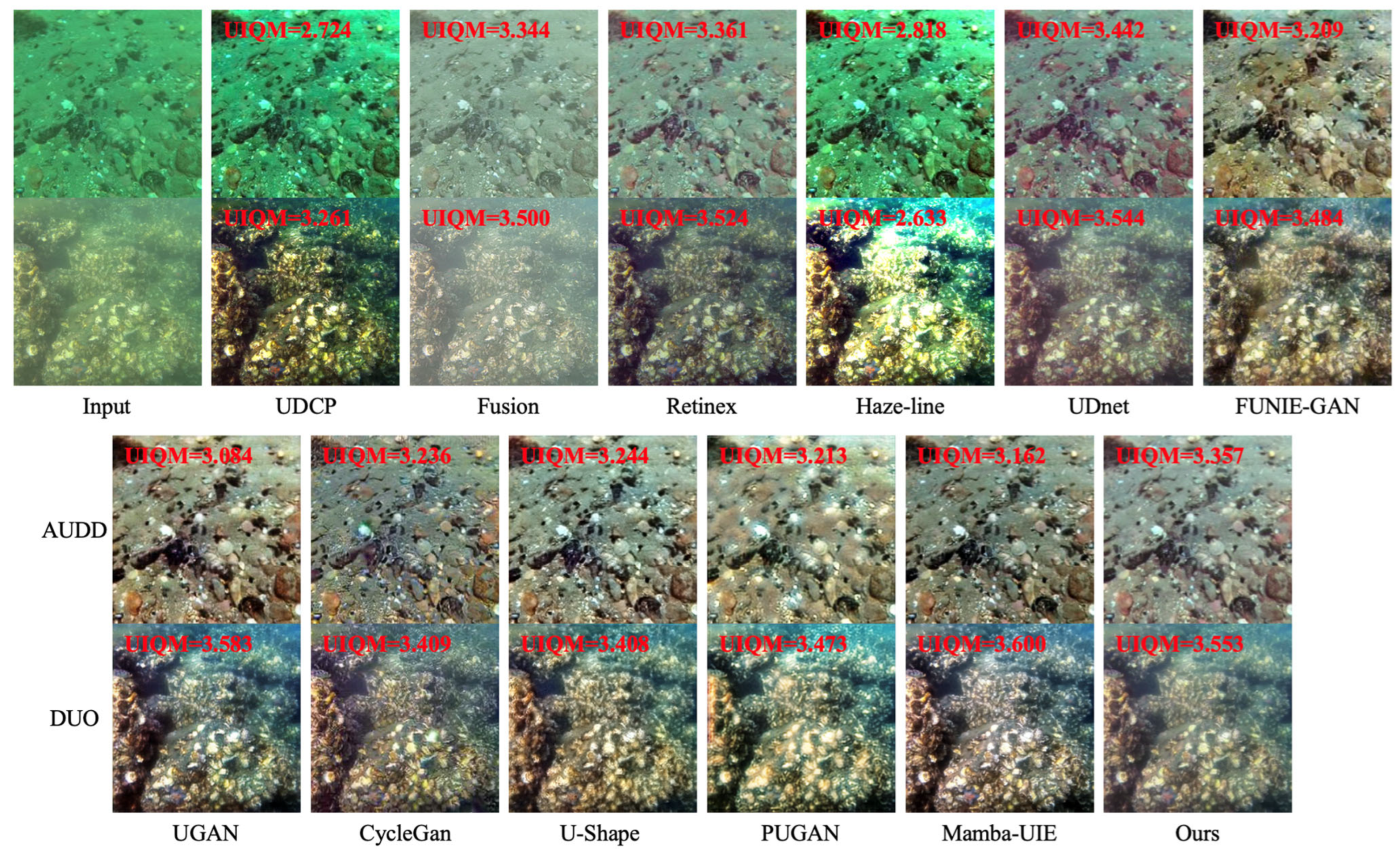
Figure 12.
Enhancement results on the AUDD and DUO datasets.
Figure 12.
Enhancement results on the AUDD and DUO datasets.
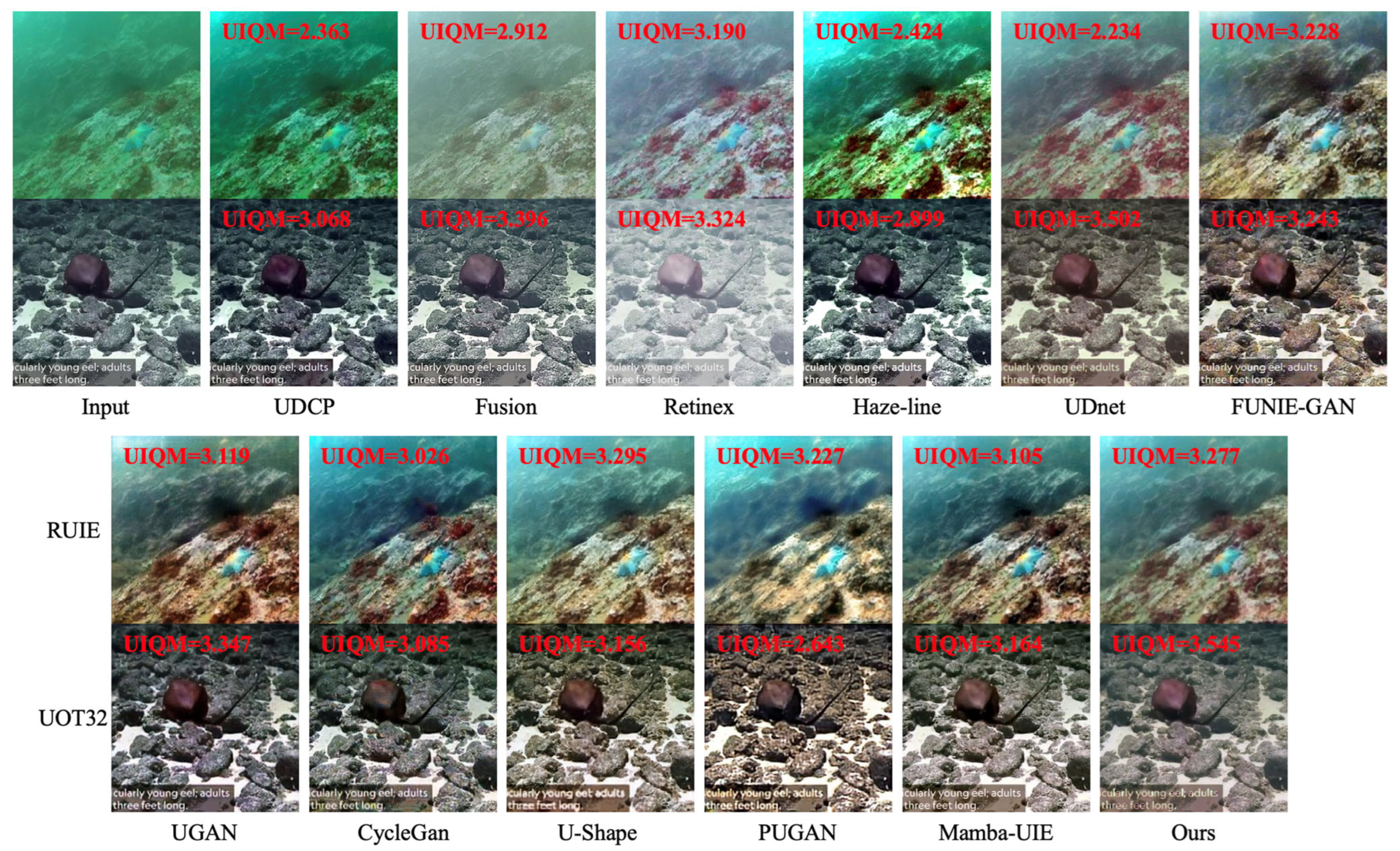
Figure 13.
Enhancement results on the RUIE and UOT32 datasets.
Figure 13.
Enhancement results on the RUIE and UOT32 datasets.
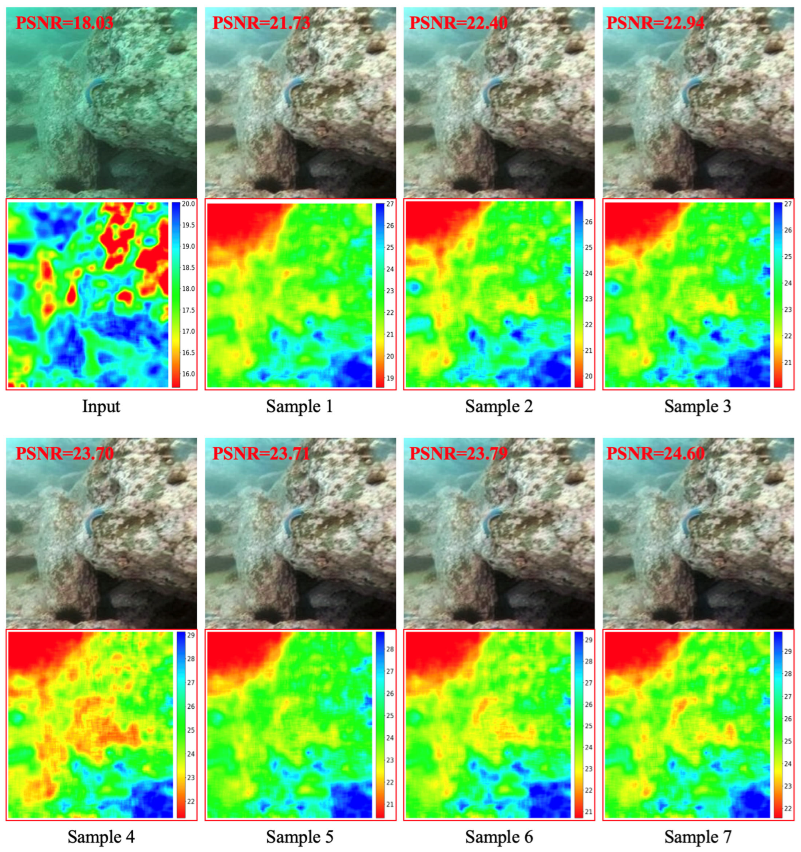
Figure 14.
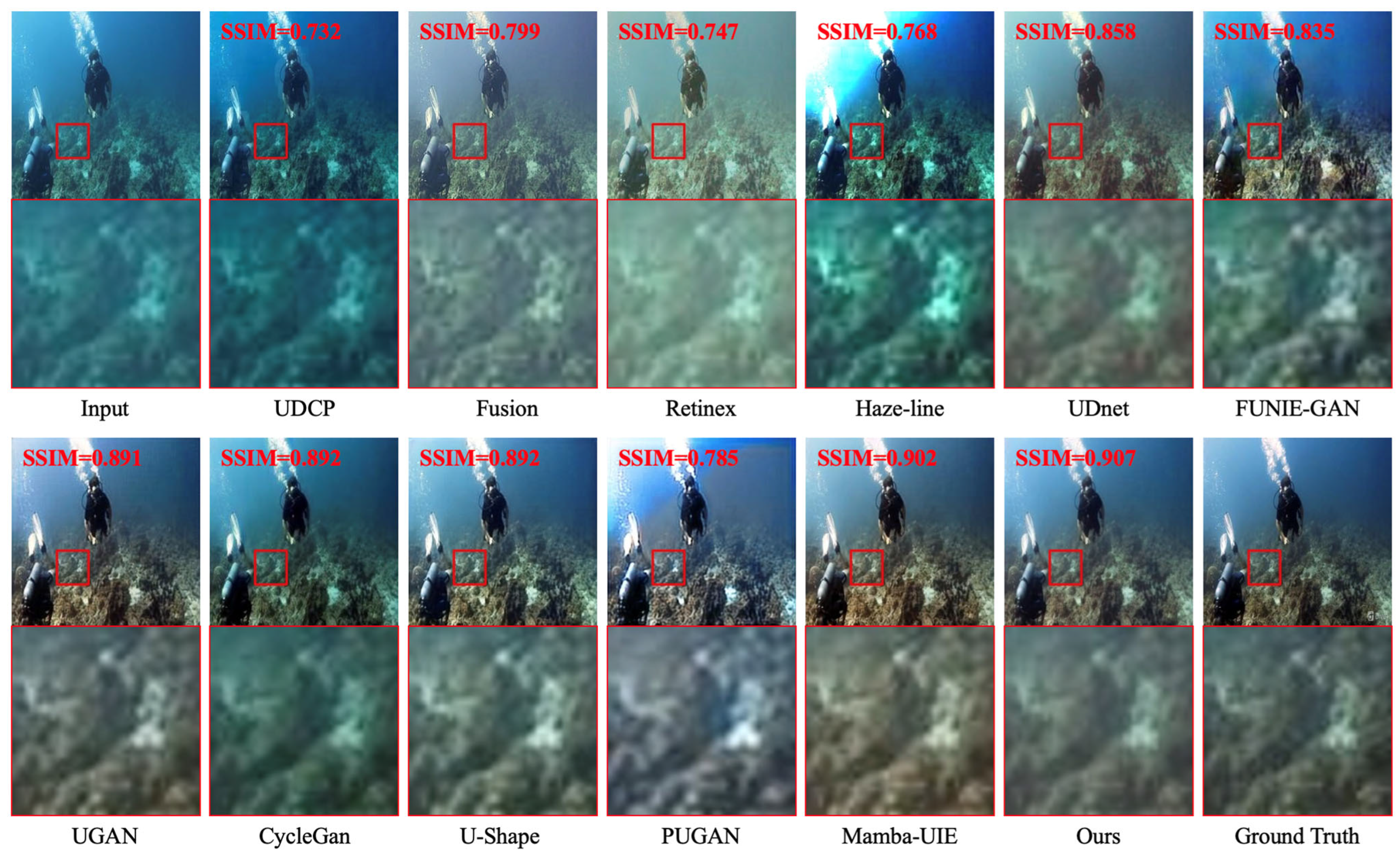
Comparison of candidate enhancement samples and the final result with corresponding PSNR heatmap visualization.
Figure 14.
Comparison of candidate enhancement samples and the final result with corresponding PSNR heatmap visualization.
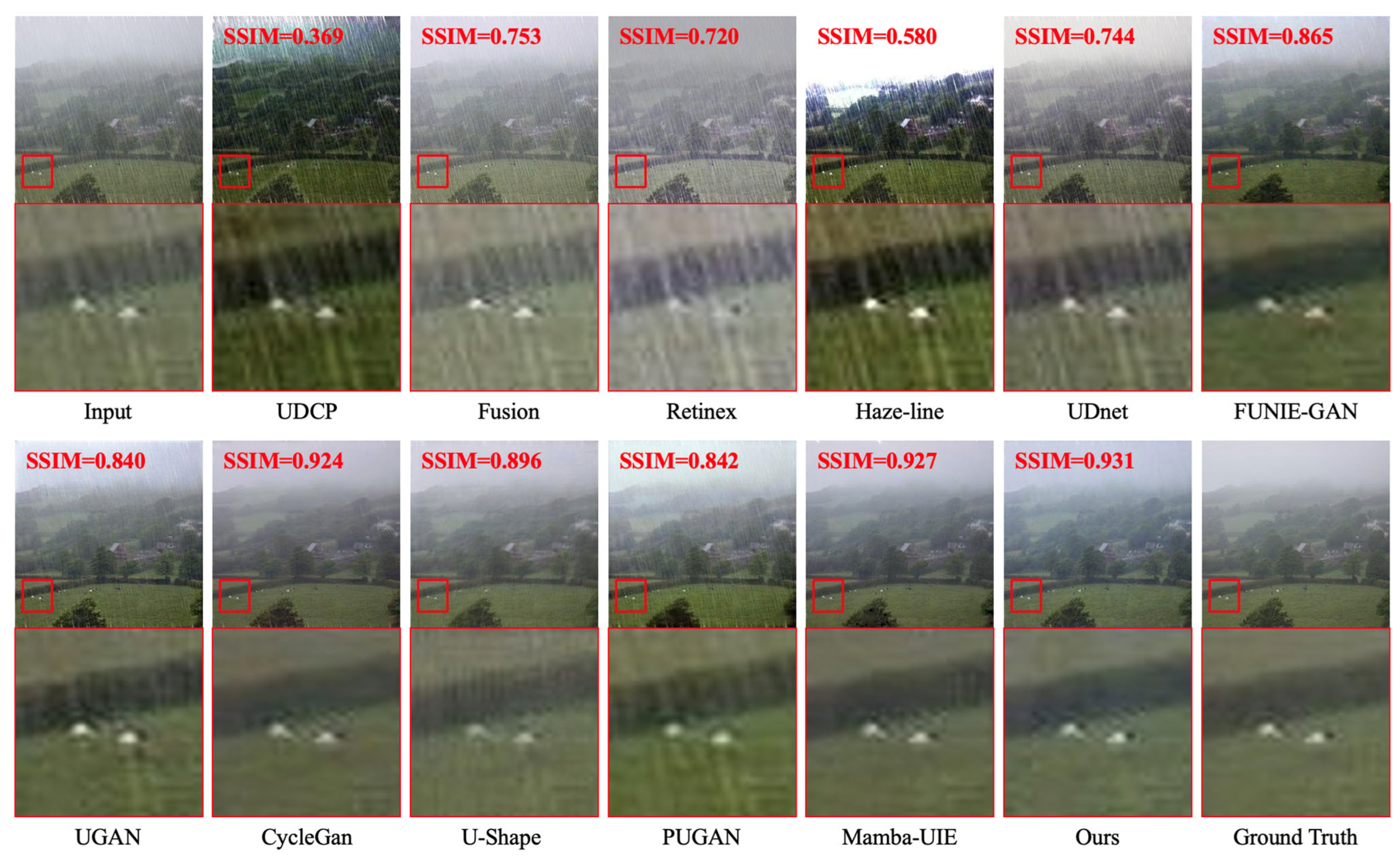
Figure 15.
Qualitative results of image deraining.
Figure 15.
Qualitative results of image deraining.
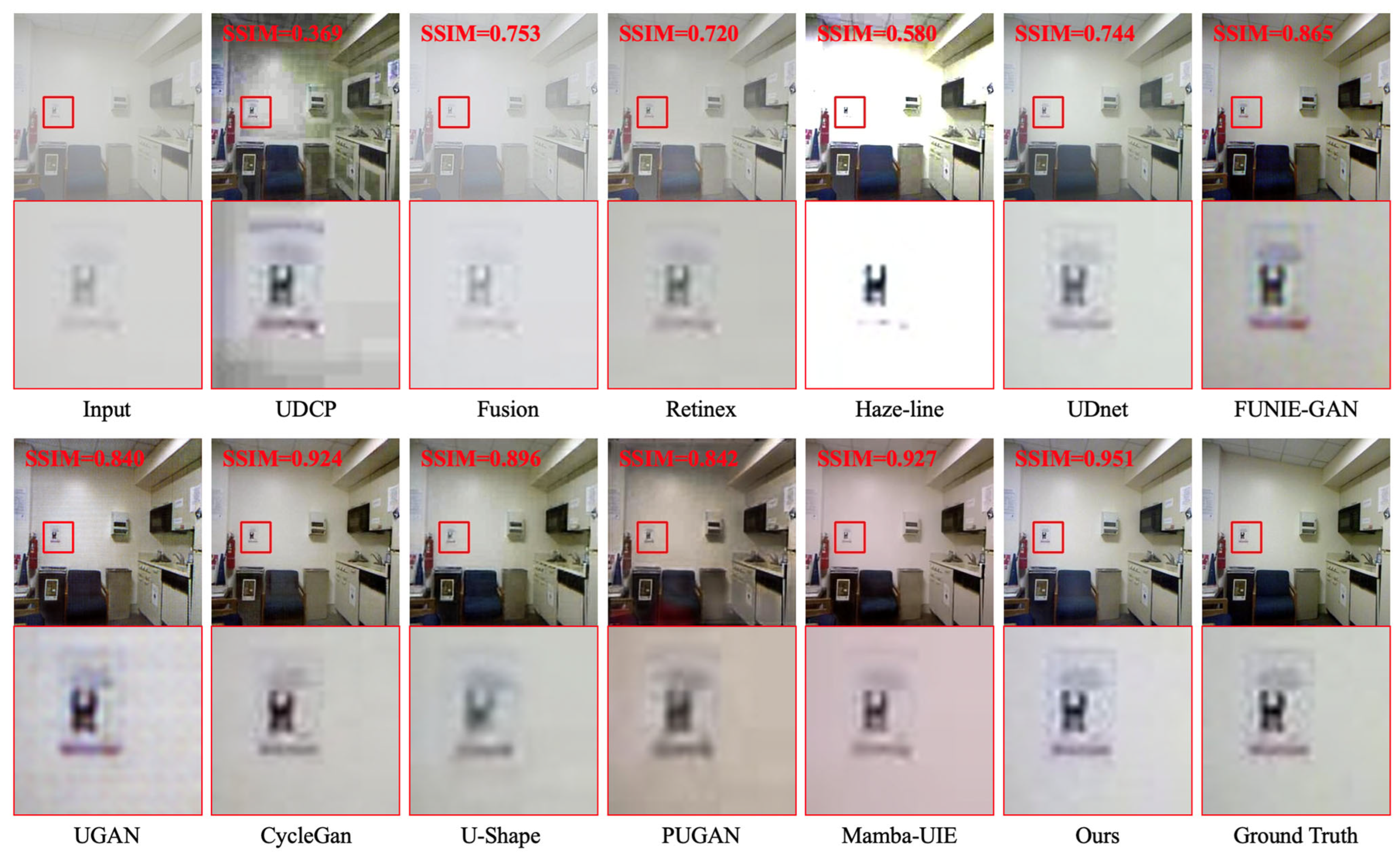
Figure 16.
Qualitative results of image dehazing.
Figure 16.
Qualitative results of image dehazing.
Table 1.
Summary of the datasets used in this study (including the numbers of image pairs).
Table 1.
Summary of the datasets used in this study (including the numbers of image pairs).
| Phase | Dataset | Reference Type | Images |
|---|
| Training | Synthetic | Paired | 800 |
| UIEB | Paired | 800 |
| Testing—Reference | EUVP | Paired | 500 |
| LSUI | Paired | 500 |
| UFO-120 | Paired | 120 |
| UIEB | Paired | 90 |
| Testing—No-reference | AUDD | Unpaired | 100 |
| DUO | Unpaired | 100 |
| RUIE | Unpaired | 100 |
| UOT32 | Unpaired | 100 |
Table 2.
Quantitative comparison on EUVP and LSUI datasets (red indicates the best performance, blue the second-best, and green the third-best values; denotes that higher values correspond to better performance; the same notation applies to remaining tables).
Table 2.
Quantitative comparison on EUVP and LSUI datasets (red indicates the best performance, blue the second-best, and green the third-best values; denotes that higher values correspond to better performance; the same notation applies to remaining tables).
| Method | EUVP | LSUI |
|---|
| | | | | |
|---|
| UDCP | 0.723 | 19.099 | 2.306 | 0.682 | 13.398 | 2.326 |
| Fusion | 0.726 | 17.087 | 3.043 | 0.773 | 17.632 | 2.941 |
| Retinex | 0.538 | 11.272 | 3.009 | 0.727 | 13.981 | 3.015 |
| Haze-line | 0.696 | 16.863 | 2.289 | 0.697 | 14.554 | 2.386 |
| UDnet | 0.722 | 19.278 | 3.170 | 0.829 | 20.712 | 3.119 |
| FUNIE-GAN | 0.701 | 18.356 | 3.045 | 0.779 | 19.146 | 3.083 |
| UGAN | 0.721 | 18.659 | 3.026 | 0.842 | 22.625 | 3.091 |
| CycleGan | 0.722 | 19.730 | 2.866 | 0.787 | 20.484 | 2.963 |
| U-Shape | 0.723 | 18.712 | 2.914 | 0.846 | 21.961 | 2.998 |
| PUGAN | 0.666 | 16.523 | 2.929 | 0.766 | 19.638 | 3.003 |
| Mamba-UIE | 0.729 | 18.326 | 2.911 | 0.877 | 22.967 | 2.949 |
| Ours | 0.735 | 19.501 | 3.051 | 0.854 | 23.044 | 3.056 |
Table 3.
Quantitative comparison on UFO-120 and UIEB datasets.
Table 3.
Quantitative comparison on UFO-120 and UIEB datasets.
| Method | UFO-120 | UIEB |
|---|
| SSIM
| PSNR
| UIQM
| | | |
|---|
| UDCP | 0.723 | 18.727 | 2.324 | 0.663 | 14.658 | 2.287 |
| Fusion | 0.733 | 17.351 | 2.976 | 0.755 | 17.262 | 2.834 |
| Retinex | 0.632 | 12.714 | 2.956 | 0.539 | 10.461 | 2.805 |
| Haze-line | 0.691 | 15.310 | 2.204 | 0.693 | 16.170 | 2.304 |
| UDnet | 0.728 | 18.844 | 3.113 | 0.773 | 18.962 | 3.000 |
| FUNIE-GAN | 0.712 | 18.727 | 2.992 | 0.768 | 18.573 | 2.968 |
| UGAN | 0.726 | 18.788 | 2.966 | 0.812 | 21.288 | 3.005 |
| CycleGan | 0.726 | 19.388 | 2.836 | 0.751 | 19.779 | 2.765 |
| U-Shape | 0.718 | 18.813 | 2.841 | 0.811 | 21.000 | 2.947 |
| PUGAN | 0.666 | 16.613 | 2.79 | 0.731 | 18.381 | 2.785 |
| Mamba-UIE | 0.731 | 18.120 | 2.845 | 0.850 | 21.781 | 2.843 |
| Ours | 0.741 | 19.359 | 2.991 | 0.810 | 20.569 | 2.980 |
Table 4.
Quantitative comparison on AUDD, DUO, RUIE, and UOT32 datasets.
Table 4.
Quantitative comparison on AUDD, DUO, RUIE, and UOT32 datasets.
| Method | AUDD | DUO | RUIE | UOT32 |
|---|
| UIQM | | | |
|---|
| UDCP | 2.674 | 3.072 | 2.617 | 3.055 |
| Fusion | 3.161 | 3.484 | 3.303 | 3.355 |
| Retinex | 3.227 | 3.417 | 3.196 | 3.084 |
| Haze-line | 2.671 | 2.582 | 2.628 | 2.907 |
| UDnet | 3.283 | 3.453 | 3.338 | 3.483 |
| FUNIE-GAN | 3.164 | 3.413 | 3.155 | 3.207 |
| UGAN | 3.151 | 3.473 | 3.213 | 3.289 |
| CycleGan | 2.943 | 3.154 | 3.073 | 3.171 |
| U-Shape | 3.209 | 3.207 | 3.150 | 3.069 |
| PUGAN | 3.102 | 3.444 | 3.194 | 2.677 |
| Mamba-UIE | 3.085 | 3.384 | 3.085 | 3.092 |
| Ours | 3.234 | 3.467 | 3.342 | 3.502 |
Table 5.
Comparison of MACs (Multiply–Accumulate Operations) and Parameters between Different Methods.
Table 5.
Comparison of MACs (Multiply–Accumulate Operations) and Parameters between Different Methods.
| | UDnet | FUNIE-GAN | UGAN | CycleGan | U-Shape | PUGAN | Mamba-UIE | Ours |
|---|
| MACs (G) | 30.150 | 10.695 | 19.820 | 56.864 | 2.985 | 75.400 | 381.569 | 211.204 |
| Params (M) | 1.402 | 7.716 | 57.169 | 11.378 | 22.817 | 101.187 | 6.046 | 17.481 |
Table 6.
Ablation Study Results: Comparison of Metrics Across Different Baselines on the LSUI Dataset.
Table 6.
Ablation Study Results: Comparison of Metrics Across Different Baselines on the LSUI Dataset.
| Multi-dimensional Feature Mapping Module | Confidence Generation Module | Probabilistic Module | | |
|---|
| √ | √ | | 0.841 | 21.963 |
| | √ | √ | 0.851 | 22.677 |
| √ | | √ | 0.851 | 22.795 |
| | | √ | 0.848 | 22.754 |
| √ | √ | √ | 0.854 | 23.044 |
Table 7.
Quantitative results for image deraining and dehazing.
lowest value.
Table 7.
Quantitative results for image deraining and dehazing.
lowest value.
| Method | Rain1400 (Deraining) | RESIDE (Dehazing) |
|---|
| | | | | |
|---|
| UDCP | 0.653 | 18.419 | 32.594 | 0.704 | 16.964 | 37.842 |
| Fusion | 0.704 | 18.501 | 31.484 | 0.632 | 10.841 | 76.369 |
| Retinex | 0.512 | 8.368 | 99.166 | 0.634 | 11.309 | 71.816 |
| Haze-line | 0.697 | 17.529 | 36.190 | 0.636 | 11.308 | 73.775 |
| UDnet | 0.733 | 20.469 | 25.653 | 0.787 | 16.726 | 41.160 |
| FUNIE-GAN | 0.842 | 26.687 | 12.247 | 0.850 | 25.938 | 13.349 |
| UGAN | 0.821 | 26.282 | 12.732 | 0.819 | 24.471 | 15.774 |
| CycleGan | 0.858 | 28.186 | 10.610 | 0.826 | 21.914 | 22.411 |
| U-Shape | 0.820 | 26.881 | 12.024 | 0.844 | 27.843 | 10.640 |
| PUGAN | 0.784 | 24.491 | 15.806 | 0.787 | 20.944 | 24.103 |
| Mamba-UIE | 0.894 | 28.229 | 10.383 | 0.897 | 26.256 | 12.844 |
| Ours | 0.900 | 28.214 | 10.421 | 0.920 | 25.987 | 13.643 |