Evaluation of Different AI-Based Wave Phase-Resolved Prediction Methods

Abstract

Ensuring the safe operation of marine structures requires accurate phase-resolved wave prediction. However, current studies mostly focus on single-model verification and lack a systematic comparison of mainstream architectures under multiple environmental factors on a unified experimental benchmark, thus offering limited guidance for engineering practice. To fill this gap, we conducted a systematic wave-tank evaluation that quantifies how sea state levels, directional spectrum, prediction distance and lead time jointly affect model accuracy. Four architectures—RNN, LSTM, GRU, and TCN—were trained on 7 × 7 probe matrices acquired under sea states levels (4–7), two directional spreading coefficients (n = 2 and 6), five prediction distances (6.7–33.3 m), and lead times of 1–30Δt. Root-mean-square error (RMSE) served as the quantitative metric. Among recurrent architectures, RNN-WP achieved the lowest high-frequency error under mild sea states (SS4, RMSE = 0.28 m), LSTM-WP delivered the best overall accuracy (SS4–5, RMSE ≤ 0.37 m), and GRU-WP excelled in the medium to high frequency band (SS4–5, RMSE ≤ 0.31 m), whereas TCN-WP remained most robust at long horizons and severe sea states (SS7, RMSE = 0.42 m). Increasing sea-state severity raised RMSE by 40–90%, while a narrower directional distribution amplified errors under extreme conditions. Prediction distance and lead time altered model ranking, confirming that nonlinearity, directional spreading, distance and temporal horizon are the dominant controlling factors for deep learning phase resolved wave prediction.

1. Introduction

Accurate wave prediction provides vessels and offshore platforms with reliable external environmental information, thereby safeguarding their operational safety. Phase-resolved wave prediction delivers instantaneous, crest-level elevation sequences, enabling more refined safety assessments for ships and offshore structures, and has thus garnered significant attention [1,2,3].

While recent AI approaches have demonstrated remarkable potential in this domain, their development is deeply rooted in, and can be seen as a direct response to the limitations of, traditional physics-based modeling. These conventional methods, while foundational, often struggle with computational expense and the need for complete boundary conditions, hindering their real-time application in complex engineering scenarios. Therefore, to fully appreciate the technical positioning and unique advantages of modern AI-based methods, it is essential to first revisit the evolution of traditional physics-based modeling. Early wave-prediction research progressed along a hydrodynamic-theory trajectory. Originating from linear wave theory and grounded in potential-flow assumptions, researchers formulated kinematic and dynamic equations. Superposition decomposed the sea state into linear wave components; imposing Laplace’s equation with boundary conditions yielded a well-posed initial–boundary-value problem [4]. This framework achieves high fidelity for small wave steepness and quasi-periodic wave fields but fails under pronounced nonlinearities. To overcome linear limitations, researchers introduced perturbation and Taylor expansions to develop second-order wave theory, retaining the potential-flow framework while incorporating nonlinear coupling terms. Dalzell [5] subsequently extended this theory to finite water depths, significantly improving predictive skill in complex bathymetry. As nonlinear wave studies advanced, High-Order Spectral (HOS) models directly solved the nonlinear evolution equation, accurately capturing high-order modes and demonstrating decisive advantages for extreme nonlinear wave fields [6]. However, the inherent field-wide numerical resolution of HOS results in exponential growth in computational complexity, precluding real-time application [7]. Mohapatra et al. [8] presented a comprehensive potential-flow-based study of a 20-hinged flexible plate validated against high-quality flume measurements, demonstrating the continued role of physics-based approaches in generating reference datasets for multi-body floating structures. To reconcile theoretical accuracy with computational efficiency, hybrid multi-dimensional strategies were developed. The governing equations were expanded to include Boussinesq [9], Green–Naghdi [10], and nonlinear Schrödinger equations [11,12,13], each tailored to specific depth regimes or dimensional extents. This enables flexible combinations of equation order and spatial dimension, enhancing robustness under severe sea states. Concurrently, computational architectures were optimized—reduced-order modeling and parallelization were adopted to shorten solution times while preserving hydrodynamic fidelity [14]. Nevertheless, these models still face inherent limitations: accurate solutions demand complete geometric boundary conditions, full initial dynamic fields, and precise radiation conditions, all of which are seldom available; consequently, sparse or missing measurements rapidly erode prediction skill. Moreover, even with reduced-order strategies, a single prediction cycle still requires hours to tens of hours, remaining fundamentally misaligned with the minute-level update cadence demanded by engineering practice. This temporal gap constitutes the principal bottleneck hindering the operational deployment of hydrodynamics-based methods.

With the iterative evolution of artificial intelligence technology, neural network architectures have continuously broken through in depth and complexity; particularly, the introduction of nonlinear activation functions has significantly enhanced models’ ability to resolve complex ocean dynamical features [15]. Data-driven neural network prediction models have gradually been applied to phase-resolved wave prediction [16], demonstrating unique advantages. Currently, typical models include ANN [17], LSTM [18], BNN [19], and CNN [20].

Zhao Yong et al. [21] analyzed and normalized typical wave test data from an island reef terrain model using LSTM neural networks, and conducted single-step and multi-step predictions of freak waves. Kim et al. [22] utilized CNN neural networks to prediction long-crested and short-crested waves, respectively, achieving good prediction results for wave peaks and troughs of long-crested waves, but lower accuracy for intermediate wave amplitudes. The prediction accuracy for short-crested waves was only 60%. Yu et al. [23] designed a nonlinear ocean wave prediction method based on Elman neural networks for nonlinear phase-resolved wave prediction problems. Duan et al. [24] proposed a long-crested wave prediction model based on ANN, which showed good accuracy in real-time prediction of phase and wave height information for long-crested waves. Law et al. [25] also used an ANN model to build a long-crested wave prediction model and analyzed the prediction range in combination with linear methods. Xuewen Ma et al. [18] (2022) verified the feasibility of LSTM models in phase-resolved prediction of short-crested waves through wave basin experiments. Jincheng Zhang et al. [19] (2022), based on variational Bayesian machine learning methods and wave flume experiments, demonstrated that for short-term wave prediction, the prediction error was 55.4% lower than linear wave theory, and the predictable area was extended by 74.6%. Liu et al. [26] fused Linear Wave Theory into PINN, yielding 13.7 s accurate forecast of irregular long-crested waves in finite depth after only 100 s upstream data and 0.13 s compute, tripling the reach of classic linear predictors for real-time OES control. Ehlers et al. [27], respectively, designed novel prediction model structures to achieve generalization optimization for wave prediction under different working conditions. However, existing research mainly focuses on testing and verification of single models, with less attention paid to the influence of factors such as different model architectures, sea states, directional spectral distributions, prediction distances, and prediction lead times on model performance.

Table 1. Overview of deep-learning, phase-resolved wave-prediction studies.

Reference	Model Architecture	Experimental Conditions	Prediction Task	Key Contribution
[21]	LSTM	Island-reef physical model, JONSWAP spectrum, uni-directional waves.	Single- and multi-step freak-wave prediction.	Demonstrated LSTM capability for short-term extreme-wave forecasting.
[22]	CNN	Wave basin: long-crested & short-crested seas, 3-D spectrum.	0–3 s wave-height regression.	Real-time mapping of spatial wave features by convolutional kernels.
[23]	Elman RNN	Numerical flume, finite depth, uni-directional waves.	Nonlinear phase-resolved forecast.	Introduced recurrent feedback to capture nonlinear phase evolution.
[25]	ANN	Towing-tank long-crested waves, sea states 3–4.	0–4 s deterministic surface-elevation time series.	Hybridized linear dispersion with ANN error correction.
[26]	LWT-PINN	Wave-tank irregular long-crested waves, steepness 0.0174–0.0349, finite water depth.	Deterministic time-history forecast of downstream surface elevation for the next 15 s.	First PINN to predict real waves; 13.7 s high-fidelity horizon with 0.13 s compute, 2.5× longer than classical linear predictor.
[27]	U-Net + Fourier Neural Operator	Synthetic 1-D radar-snapshot data, multiple historic time slices.	Phase-resolved reconstruction from sparse radar snapshots.	Replaced heavy optimization with NN mapping; FNO learns global wave-physics relationship in Fourier space, yielding real-time capable and sea-state-robust reconstruction.

summarizes the model architectures, experimental conditions, prediction tasks and key contributions of the studies reviewed. Collectively, these works demonstrate the feasibility of using deep learning methods for phase-resolved wave modeling under diverse settings. However, a critical gap remains: existing studies predominantly focus on introducing novel architectures or optimizing data for specific scenarios, leading to fragmented conclusions that are difficult to compare directly due to differing experimental conditions. Consequently, a systematic, head-to-head comparison of mainstream architectures on a unified benchmark is still lacking, leaving practitioners without clear guidance on model selection for specific operational contexts. To bridge this gap, the present study conducts a comprehensive evaluation of four mainstream networks RNN, LSTM, GRU, and TCN by training and testing them on the same experimental dataset across a wide range of operational conditions. This study not only reaffirms the strong potential of deep learning models in wave prediction but also elucidates the intricate interplay between model architecture and environmental factors. We quantitatively investigated the effect of sea-state severity, directional spreading, prediction distance, and lead time step on the model prediction performance. By uncovering these context-dependent performance patterns, our research provides actionable, quantitative guidance for architecture selection, thereby offering a robust performance assessment for engineering applications and a solid foundation for future research aimed at targeted optimization.

The paper is organized as follows. Section 2 presents the methodology and theoretical foundation of the phase-resolved intelligent wave-prediction framework. Section 3 describes the data sources and error assessment metrics. Section 4 investigates the individual and combined effects of sea state, directional spreading, prediction distance, and lead-time step on the predictive accuracy of the four models, providing a comprehensive analysis of the results.

2. Data and Error Evaluation Methods

2.1. Data Sources

The wave data acquisition experiment was conducted in the deep-water tank (50 m length × 30 m width × 10 m depth, Harbin Engineering University, Harbin, China), equipped with a wave generator and towing carriage. Concurrent studies have employed motor-driven emulators to reproduce WEC motion in the laboratory for control and power-testing purposes [28]. Figure 1 illustrates the experimental setup used to measure wave propagation characteristics. The left diagram details the relative positions of the wave maker and wave probes, including probe numbering. The right diagram depicts wave propagation and actual probe placement. A 7 × 7 wave probe matrix (1.2 m × 1.2 m) was deployed with 0.2 m spacing between probes. During wave generation, the triangular wave field region exhibits consistency with the wave maker’s generated spectrum, optimally reflecting the defined wave characteristics. Hence, the probe matrix was positioned within this triangular area. The wave elevation data were collected using the YWH200-D digital wave gauge, which has a measurement accuracy of ±0.15% full scale (FS) and a response time of ≤1 ms. Prior to the experiments, all sensors were calibrated to ensure correct zero referencing and linearity across the measurement range. The sampling frequency was set to 100 Hz, which is sufficient to capture the temporal characteristics of the wave field and meets the uncertainty requirements of this study.

The experimental procedure is as follows: First, the wave maker generates waves using the JONSWAP spectrum (Equation (1)) as the target energy spectrum, with spectral peak enhancement factor γ = 2.2 (a lower value is used because γ = 3.3 would over-concentrate energy around fp and exceed the present wave-maker stroke limit). Concurrently, a directional distribution function (Equation (2)) simulates wave directionality, employing directional coefficients n = 2 and n = 6. Experimental conditions span sea states 4–7, which correspond to typical environmental loading scenarios widely documented in offshore and marine engineering literature. Upon propagation through the tank, waves reach the predetermined wave probe matrix position, where probes record wave heights. Specific experimental conditions are summarized in

Table 2. Test Condition.

Sea State Level	Significant Wave Height (m)	Spectral Peak Frequency (s)
4	2/2.1	9.5
5	3.5/3.7	10
6	5/5.34	11
7	6/6.34	12

Note: The term ‘Sea State Level’ follows the WMO nomenclature (WMO-No. 558, 2018 [29]) where levels 4–7 correspond to the indicated ranges of significant wave height. This classification is standard in wave-tank and ocean-engineering literature and allows direct comparison with previous studies.

:

$$S(\omega )=0.658{\displaystyle \frac{173H_s^2}{T_1^4{\omega }^5}}\exp \left(-{\displaystyle \frac{691}{T_1^4{\omega }^5}}\right){\gamma }^{\exp \left(-{\displaystyle \frac{1}{2{\sigma }^2}}{\left({\displaystyle \frac{T_1\omega }{4.85}}-1\right)}^2\right)}$$

(1)

$${\omega }_0={\displaystyle \frac{4.85}{T_1}}\left\{\begin{array}{c}\begin{array}{cc}\sigma =0.07& \omega \le {\omega }_0\end{array}\\ \begin{array}{cc}\sigma =0.09& \omega >{\omega }_0\end{array}\end{array}\right.$$

(2)

$$G(\omega ,\theta )=C(n){\cos }^{2n}\theta$$

(3)

$$C(n)={\displaystyle \frac{1}{\sqrt{\pi }}}{\displaystyle \frac{\Gamma (n+1)}{\Gamma (n+\frac{1}{2})}}$$

(4)

2.2. Error Evaluation Methods

To evaluate discrepancies in wave prediction performance across influencing factors and models, this study employs Root Mean Square Error (RMSE) as the performance metric. RMSE, a standard error metric in time series prediction, quantifies prediction accuracy across the entire temporal segment. The RMSE calculation is defined as follows:

$$\mathrm{RMSE}=\sqrt{{\displaystyle \frac{{\displaystyle \sum _{N_{pre}}{\left({\eta }_i^{pre}-{\eta }_i^{mea}\right)}^2}}{N_{pre}}}}$$

(5)

Here, RMSE denotes the Root Mean Square Error, ${\eta }_i^{pre}$ represents the predictedwave surface at time i, ${\eta }_i^{mea}$ is the observed wave surface at time i, and $N_{pre}$ is the total number of points in the error calculation. Unless otherwise specified, all prediction errors reported in tables and figures refer to Root Mean Square Error (RMSE) in meters.

3. Method and Theory

3.1. Physical Basis of Phase-Resolved Wave Intelligent Prediction

Intelligent prediction models and traditional hydrodynamic methods are fundamentally grounded in identical physical principles; both aim to capture wave propagation patterns within the spatiotemporal domain. The distinction resides in their implementation: whereas traditional methods numerically solve wave differential equations, intelligent models employ neural networks to implicitly learn the feature-mapping relationship characterizing the physical process. This circumvents the computationally intensive partial-differential-equation (PDE) solution process inherent in conventional techniques, thereby substantially enhancing computational efficiency.

Assuming one-dimensional wave propagation and invoking the linear wave model, the two-dimensional wave surface elevation at a given spatial location can be expressed in the following integral form:

$$\eta (x,t)={\displaystyle {\int }_0^{\infty }a}(\omega )\cos (k(\omega )x-\omega t+\phi (\omega ))d\omega$$

(6)

$$k(\omega )=\mathrm{sign}(\omega )·{\displaystyle \raisebox{1ex}{${\omega }^2$}\!\left/ \!\raisebox{-1ex}{$g$}\right.}$$

(7)

$$\mathrm{sign}(\omega )=\left\{\begin{array}{ll}1\hfill & \omega >0\hfill \\ 0\hfill & \omega =0\hfill \\ -1\hfill & \omega <0\hfill \end{array}\right.$$

(8)

To establish the relationship between upstream and downstream wave positions, as illustrated in Figure 2, we apply Euler’s formula to express the integral as the sum of two integrals over 0 to ∞ and −∞ to 0.

$$\begin{array}{ll}\eta (x,t)& ={\displaystyle {\int }_0^{\infty }a}(\omega )\cos (k(\omega )x-\alpha t+\phi (\omega ))d\omega \\ & ={\displaystyle {\int }_0^{\infty }\frac{1}{2}}\alpha (\omega )e^{i[(k(\omega )x-\omega t)+\phi (\omega )]}d\omega +{\displaystyle {\int }_0^{\infty }\frac{1}{2}}\alpha (-\omega )e^{-i[(k(\omega )x-\omega t)+\phi (\omega )]}d\omega \\ & ={\displaystyle {\int }_0^{\infty }\frac{1}{2}}\alpha (\omega )e^{i[\phi (\omega )]}{e}^{i[k(\omega )x-\omega t]}d\omega +{\displaystyle {\int }_0^{\infty }\frac{1}{2}}\alpha (\omega )e^{-i[\phi (\omega )]}{e}^{-i[-k(\omega )x-\omega t]}d\omega \\ & ={\displaystyle {\int }_0^{\infty }\frac{1}{2}}\alpha (\omega )e^{i[\phi (\omega )]}{e}^{i[k(\omega )x-\omega t]}d\omega +{\displaystyle {\int }_0^{-\infty }\frac{1}{2}}\alpha (-\omega )e^{-i\phi (-\omega )}{e}^{-i[-k(-\omega )x+\omega t]}d\left(-\omega \right)\\ & ={\displaystyle {\int }_0^{\infty }\frac{1}{2}}a(\omega )e^{i\phi (\omega )}{e}^{i(k(\omega )x-\alpha t)}d\omega +{\displaystyle {\int }_{-\infty }^0-}{\displaystyle \frac{1}{2}}a(-\omega )e^{-i\phi (-\omega )}{e}^{-i(k(-\omega )x+\alpha t)}d(-\omega )\end{array}$$

(9)

The physical meaning of the dispersion relation, added-mass and radiation-damping coefficients, as well as the Cummins memory integral appearing in Equations (6)–(10), is detailed in [30]. It is evident that the difference in the spatiotemporal phase term between the two integrals primarily resides in k(ω). For the second integral, when ω ≤ 0, the term −k(−ω) involves the sign function sign(−ω), which is equivalent by definition to sign(ω) for ω ≥ 0. Consequently, the term −k(−ω) in the second integral can be expressed as k(ω):

$$-k(-\omega )=-\mathrm{sign}(-\omega )·{(-\omega )}^2/g=-{\omega }^2/g=k(\omega )\hspace{1em}(\omega <0)$$

(10)

Thus, the two integrals in the wave surface expression are consolidated into a single integral:

$$\eta (x,t)={\displaystyle {\int }_0^{\infty }a}(\omega )\cos (k(\omega )x-\omega t+\phi (\omega ))d\omega ={\displaystyle {\int }_{-\infty }^{\infty }A}(\omega )e^{i(k(\omega )x-\omega t)}d\omega$$

(11)

$$A\left(\omega \right)=\left\{\begin{array}{cc}\frac{1}{2}a\left(\omega \right)e^{i\phi \left(\omega \right)},& \omega \ge 0\\ \frac{1}{2}a\left(-\omega \right)e^{-i\phi \left(-\omega \right)},& \omega <0\end{array}\right.$$

(12)

The amplitude A(ω) possesses even symmetry, whereas the phase exhibits odd symmetry:

$$\left|A\left(\omega \right)\right|=\left|A\left(-\omega \right)\right|$$

(13)

$$\angle A(-\omega )=-\angle A(\omega )$$

(14)

At x = 0, the expression reduces to:

$$\eta (0,t)={\displaystyle {\int }_{-\infty }^{\infty }A(\omega )e^{i(-\omega t)}d\omega }$$

(15)

The form corresponds to the Fourier forward transform of A(ω). Here, η(0,t) functions as the mapping function of A(ω). Accordingly, the inverse Fourier transform is employed to retrieve A(ω).

$${\displaystyle \frac{1}{2\pi }}{\int }_{-\infty }^{\infty }\eta (0,t)e^{i\omega t}d\omega ={\displaystyle \frac{1}{2\pi }}{\int }_{-\infty }^{\infty }\left({\int }_{-\infty }^{\infty }A({\omega }^{\prime })e^{i(-{\omega }^{\prime }t)}d{\omega }^{\prime }\right)e^{i\omega t}d\omega =A(\omega )$$

(16)

Substituting A(ω) into Equation (11) results in

$$\begin{array}{ll}\eta (x,t)& ={\int }_{-\infty }^{\infty }{\displaystyle \frac{1}{2\pi }}{\int }_{-\infty }^{\infty }\eta (0,\tau )d\tau e^{i(k(\omega )x-\omega (t-\tau ))}d\omega \\ & ={\int }_{-\infty }^{\infty }\eta (0,\tau ){\displaystyle \frac{1}{2\pi }}{\int }_{-\infty }^{\infty }{e}^{i(k(\omega )x-\omega (t-\tau ))}d\tau d\omega \\ & ={\int }_{-\infty }^{\infty }\eta (0,\tau )g(t-\tau ,x)d\tau \end{array}$$

(17)

Equation (17) establishes that the wave at position x is represented by the wave at position x = 0, referring to the discrete form of this equation by Belmont [31]; assuming there are N data points, it can be transformed into the following form:

$$\eta \left(x,pdt\right)={\displaystyle \frac{1}{N}}{\displaystyle \sum _{l=p-N}^p\eta \left(0,ldt\right)g\left[\left(p-l\right)dt,x\right]}$$

(18)

Thereby, the physical foundation for the AI-based wave-prediction model is furnished.

3.2. Overview of Phase-Resolved Wave Intelligent Prediction Model

3.2.1. Recurrent Neural Network for Wave Prediction (RNN-WP)

RNN fundamentally functions as an autoregressive model. Its core mechanism relies on a hidden state serving as an internal memory unit. This architecture enables the output at each time step to depend not only on the current input but also on the hidden state from the preceding time step, thereby facilitating the recurrent processing of sequential information. Consequently, RNNs must compute serially in the order of time steps; the calculation at any given moment depends on the historical information encapsulated in the hidden state from all prior moments. This characteristic renders RNNs inherently suitable for handling variable-length sequences and provides significant advantages in problems involving temporal dependencies, leading to their widespread adoption across multiple domains. The primary structure is illustrated in Figure 3 below:

The forward propagation of the Recurrent Neural Network (RNN) [32] adheres strictly to this structure. At time step t:

$$h^{(t)}=\varphi (U{x}^{(t)}+W{h}^{(t-1)}+b)$$

(19)

Here, $\varphi \left(·\right)$ represents the activation function, typically implemented as the hyperbolic tangent (tanh), and b denotes the bias vector. Thus, the output at time step t is expressed as:

$$o^{(t)}=V{h}^{(t)}+c$$

(20)

Following the aforementioned recurrent structure, the final prediction output is obtained as:

$${\widehat{y}}^{(t)}=\sigma (o^{(t)})$$

(21)

Here, $\sigma (·)$ represents the activation function, commonly implemented as the softmax function.

Owing to the gradient vanishing and explosion issues that afflict RNNs when processing long sequences, researchers have developed two enhanced recurrent neural network architectures: Long Short-Term Memory (LSTM) and Gated Recurrent Unit (GRU). By leveraging gating mechanisms, these architectures more effectively regulate information flow across time steps. This significantly mitigates the gradient vanishing and explosion problems while concurrently enhancing model performance on long sequences.

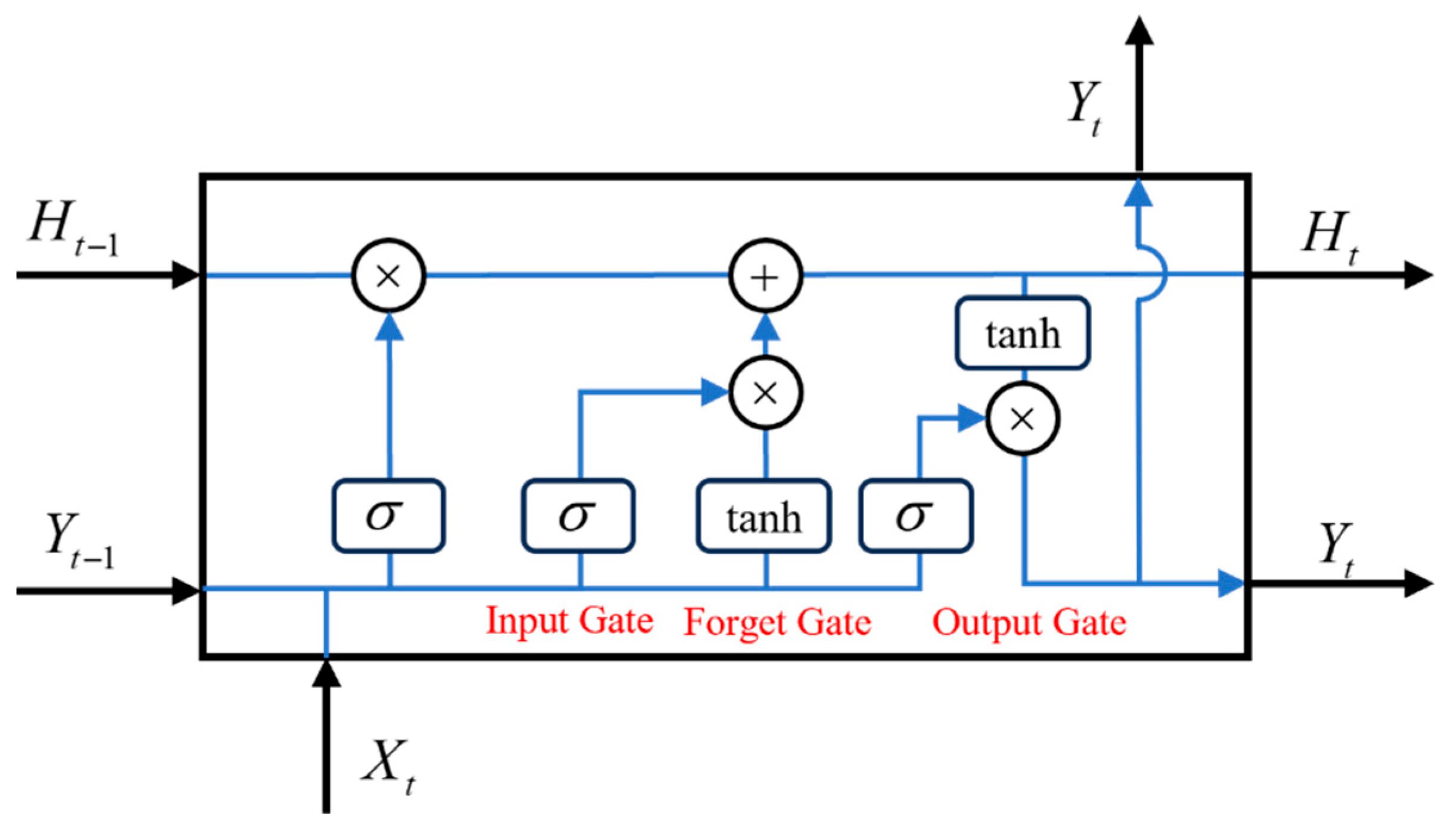
The LSTM (Long Short-Term Memory) [33] network was introduced by Hochreiter and Schmidhuber in 1997. Its core concept involves the introduction of a “gate” mechanism to control the flow of information within the cell state. The LSTM network comprises three gates: the forget gate, the input gate, and the output gate. The forget gate determines which information from the previous time step’s cell state should be discarded. The input gate regulates which information from the current time step’s input should be incorporated into the cell state. The output gate controls which information from the cell state should be passed on to the next time step. Through these gating mechanisms, the LSTM network can more effectively learn and retain crucial information in long sequences, thereby enhancing model performance in long-sequence tasks. The network structure is depicted in Figure 4 below:

In the mathematical representation of the LSTM network, we consider h hidden units, a batch size of n, and d input features. At time step t, the input is denoted as X_t, the hidden state from the previous time step is H_t−1, the input gate is I_t, the forget gate is F_t, and the output gate is O_t. The governing equations are as follows:

$$I_t=\sigma (X_t{W}_{xi}+H_{t-1}{W}_{hi}+b_i)$$

(22)

$$F_t=\sigma (X_t{W}_{xf}+H_{t-1}{W}_{hf}+b_f)$$

(23)

$$O_t=\sigma (X_t{W}_{xo}+H_{t-1}{W}_{ho}+b_o)$$

(24)

The weight parameters W denote the input weight matrices, respectively, b represents the bias vector, and $\sigma \left(·\right)$ is the activation function defined as the sigmoid function.

The computational formula for the memory cell in the LSTM is as follows:

$$C_t=F_t\odot C_{t-1}+I_t\odot \tanh (X_t{W}_{xc}+H_{t-1}{W}_{hc}+b_c)$$

(25)

Here, the forget gate F_t determines which information from the previous time step’s memory cell state C_t−1 needs to be forgotten, and the input gate I_t decides how much of the new information at the current time step needs to be added to the memory cell. Ultimately, the output of this structure is the hidden state H_t, which is produced by the output gate O_t gating the hyperbolic tangent of the current cell state C_t.

$$H_t=O_t\odot \tanh (C_t)$$

(26)

$${\hat{\mathrm{y}}}_t=W_{hy}{H}_t+b_y$$

(27)

The final prediction is generated by projecting the final hidden state H_t through a linear transformation.

The Gated Recurrent Unit (GRU) [34] network represents a streamlined variant of the LSTM architecture. It consolidates the forget and input gates of LSTM into a unified update gate, while incorporating a reset gate to regulate temporal information flow. The update gate governs the retention of prior hidden state information versus its update with new content, whereas the reset gate determines the integration of current input with the previous hidden state.

This structural simplification enhances computational efficiency while effectively mitigating vanishing and exploding gradient issues. The GRU architecture is depicted as follows (Figure 5):

In the mathematical formulation of the GRU network, the architecture comprises h hidden units, a batch size of n, and dd input features. At time step t, the input is denoted as X_t, the hidden state from the previous time step is H_t−1, the reset gate is R_t, and the update gate is Z_t. The computational formulas are defined as follows:

$$R_t=\sigma (X_t{W}_{xr}+H_{t-1}{W}_{hr}+b_r)$$

(28)

$$Z_t=\sigma (X_t{W}_{xz}+H_{t-1}{W}_{hz}+b_z)$$

(29)

Here, W denotes the weight matrices, b represents the bias vector, and $\sigma \left(·\right)$ is the activation function (sigmoid in this work). The hidden state is computed as follows:

$$H_t=Z_t\odot H_{t-1}+\left(1-Z_t\right)\odot \tanh (X_t{W}_{xh}+(R_t\odot H_{t-1})W_{hh}+b_h)$$

(30)

The update gate Z_t regulates the contribution of the previous hidden state H_t−1 and the candidate state $\tanh (X_t{W}_{xh}+(R_t\odot H_{t-1})W_{hh}+b_h)$ to the current hidden state H_t. Subsequently, a linear transformation is applied to H_t to generate the final prediction.

$${\hat{\mathrm{y}}}_t=W_{hy}{H}_t+b_y$$

(31)

3.2.2. Temporal Convolutional Network for Wave Prediction (TCN-WP)

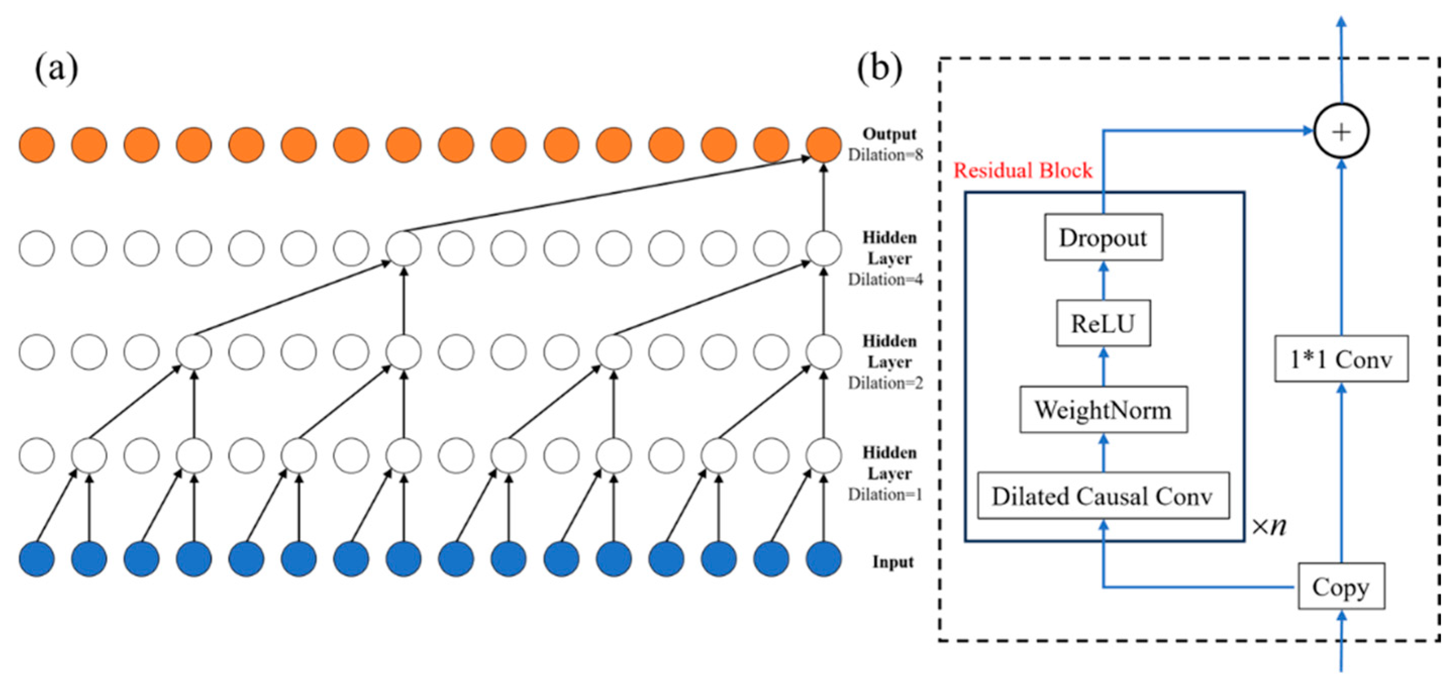
TCN [35] utilizes hierarchical convolutional layers to extract features from sequential data, making it highly effective for sequence modeling and prediction tasks. Figure 6 illustrates the TCN architecture with a kernel size of 2 and dilation factors exponentially increasing as [1, 2, 4, 8]. In this setup, each layer receives inputs from non-consecutive time steps of the preceding layer. The dilation factor dictates the interval between these input points, enabling the network to expand its receptive field exponentially with depth. This design allows the TCN to capture long-range dependencies in the input sequence efficiently.

To ensure temporal alignment between input and output sequences, the TCN employs a 1-D CNN architecture. Traditional convolution operations reduce output sequence length due to kernel sliding, violating the TCN’s core design principle of temporal length preservation. To resolve this, the TCN implements symmetric zero-padding by adding sufficient zeros to both ends of the input sequence. This strategy ensures input-output length equivalence across all hidden layers while maintaining consistent time-step correspondence.

While dilated causal convolutions enable the construction of networks with large receptive fields using a relatively small number of layers, very deep architectures—necessary for modeling highly complex sequences—are still susceptible to gradient-related problems, such as vanishing or exploding gradients, and network degradation. To address these challenges, the TCN architecture is built upon a foundation of residual blocks. These blocks facilitate the training of deeper networks by providing a shortcut for the gradient to flow, thereby mitigating degradation and improving generalization. A residual block computes the transformation F(x) and adds it to the input x. To ensure the addition is valid when the dimensions of x and F(x) differ (e.g., in the number of channels), a 1 × 1 convolution is applied to the input pathway x to match the dimensions of the output pathway F(x).

4. Results and Analysis

This section provides a detailed analysis of the performance of four proposed machine learning methods (RNN-WP, LSTM-WP, GRU-WP, TCN-WP) in prediction phase-resolved wave surfaces of wave fields under varying conditions.

First, the models’ prediction performance across different sea states is evaluated, and the impact of sea state variations on prediction errors is discussed (Section 4.1). Subsequently, the influence of directional spectrum distributions on model performance is examined, with explanations for error variations due to spectral changes (Section 4.2). Next, performance at different prediction distances is analyzed, addressing the effect of distance changes on prediction errors (Section 4.3). Finally, performance under varying lead prediction steps is investigated, elucidating the impact of step changes on errors (Section 4.4).

Tank experimental data are utilized for model training and prediction. To ensure data quality, the initial 40 s of wave generation and final 40 s of wave absorption are excluded; data from the middle period of stable wave propagation serve as valid inputs.

4.1. Influence of Sea State

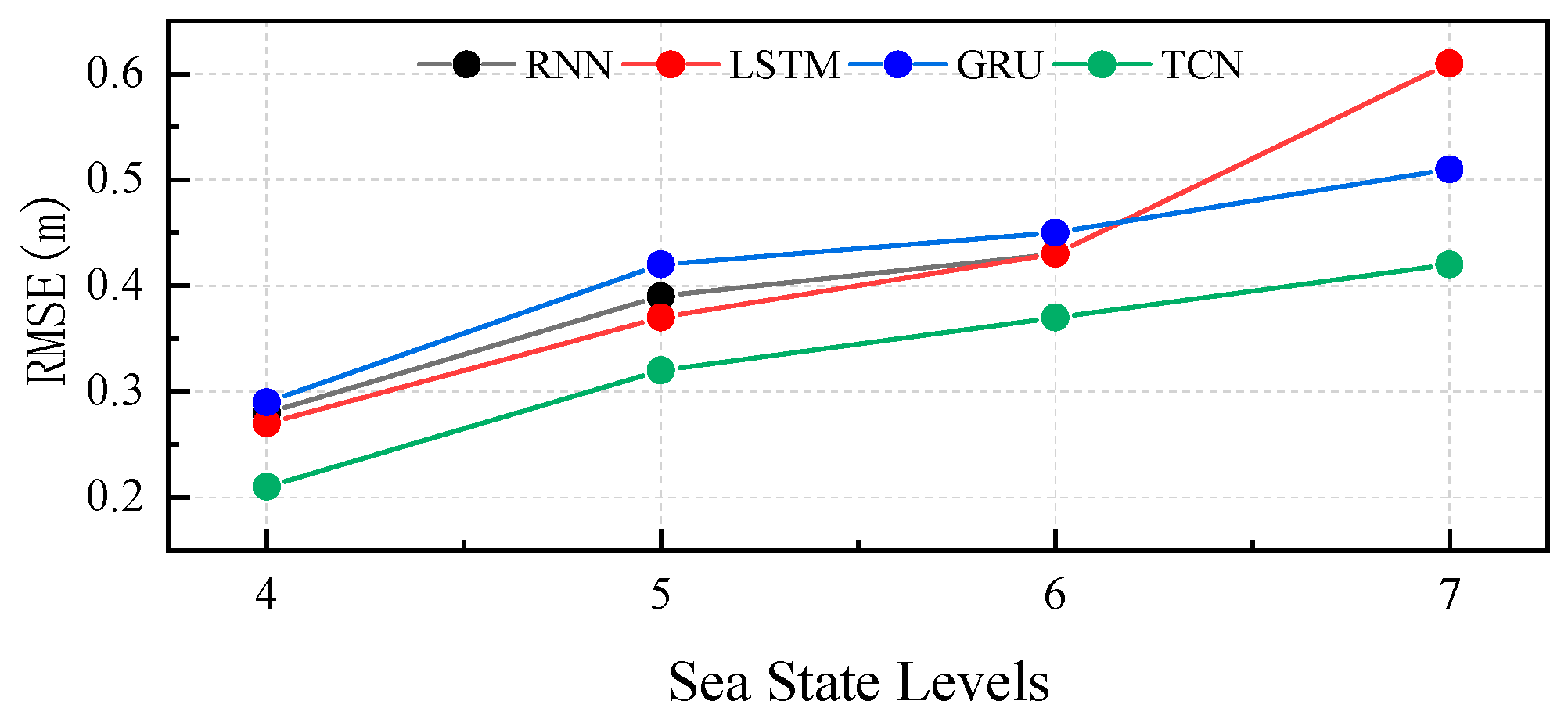
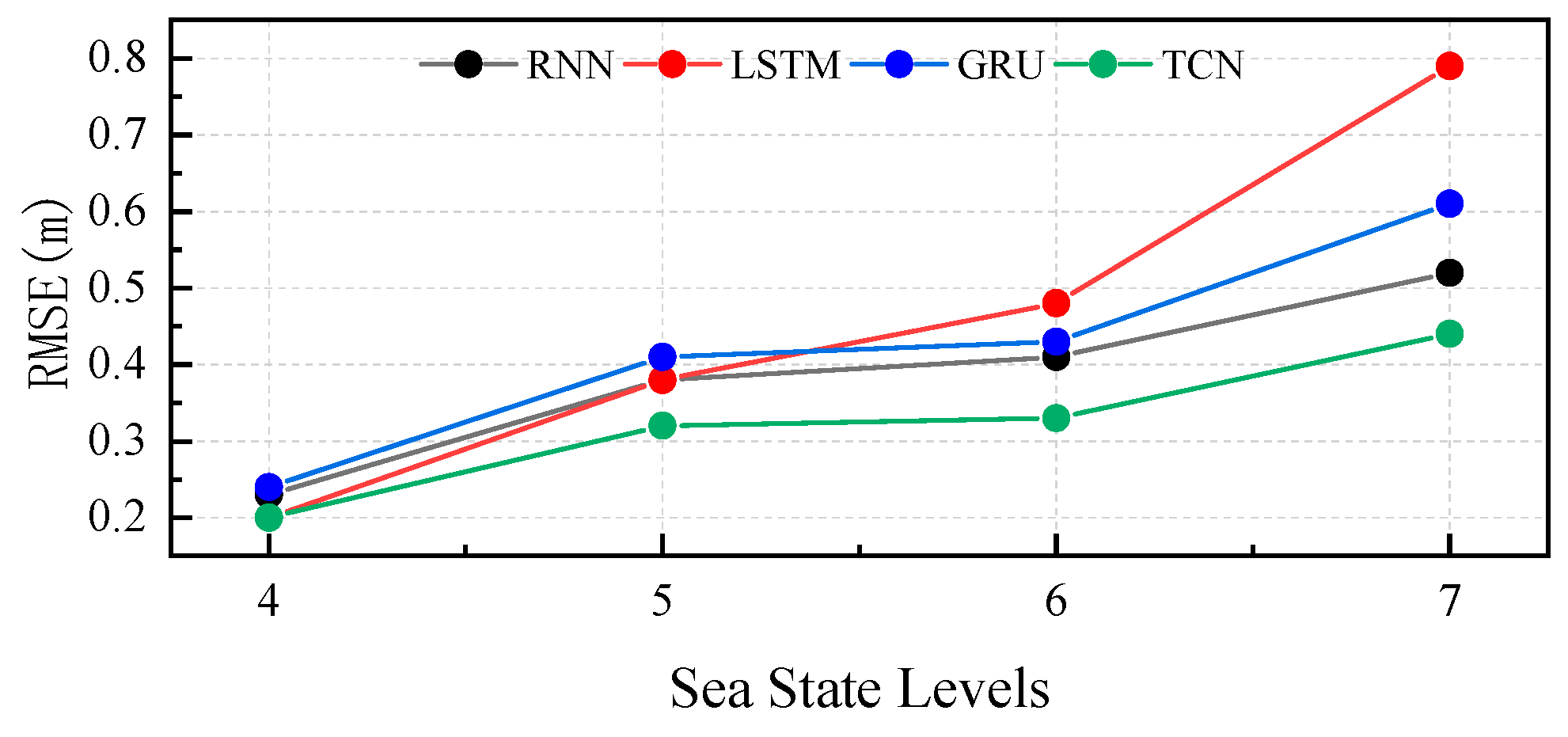
Wave nonlinearity scales monotonically with sea-state severity. To quantify discrepancies in predictive accuracy of phase-resolving wave models across varying sea states, four candidate architectures were trained independently on datasets partitioned by sea-state severity. The directional spectrum coefficient was fixed at n = 2 for all experiments. For each sea state (SS4–SS7), multivariate inputs comprised the first 150 temporal steps of wave elevation data from gauges 1, 14, 15, 28, 29, 42, and 43, targeting wave surface elevation at gauge 22 with a 10-step lead time. Comparative error metrics across SS4–SS7 are presented in

Table 3. Quantitative Prediction Errors of the Four Models Across Four Sea-State Levels.

	Model Names	RNN	LSTM	GRU	TCN
Sea State Levels
4		0.28	0.27	0.29	0.21
5		0.39	0.37	0.42	0.32
6		0.43	0.43	0.45	0.37
7		0.61	0.61	0.51	0.42

and Figure 7.

Overall, with increasing sea-state severity, wave nonlinearity intensifies markedly and the prediction errors of the four models rise correspondingly. This indicates that, under more complex and severe sea states, the predictive performance of all models is negatively affected to varying degrees. Within any single sea state, however, the models exhibit distinct relative strengths. Detailed comparative analyses of the four models under specific sea states are therefore presented below.

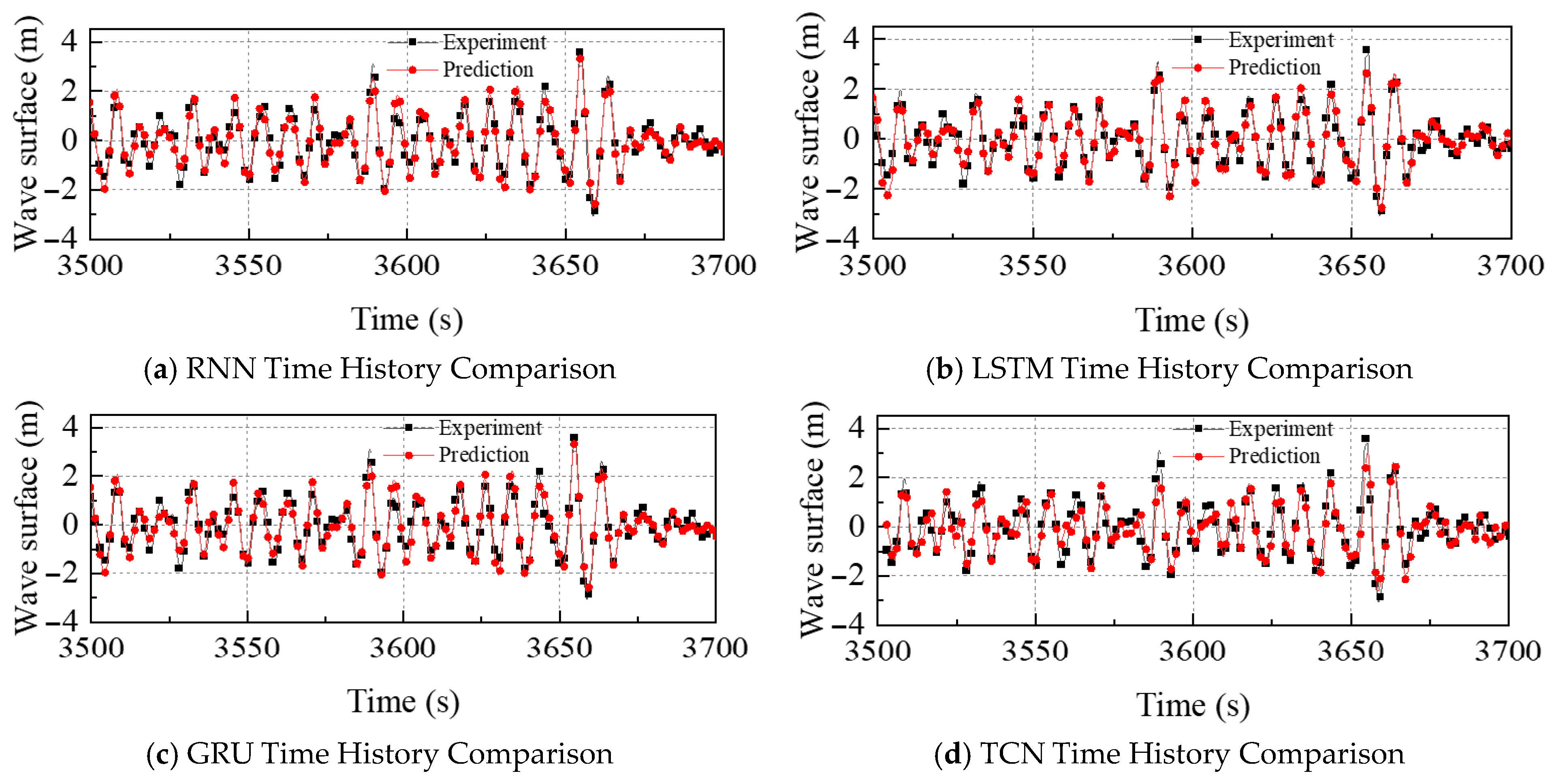
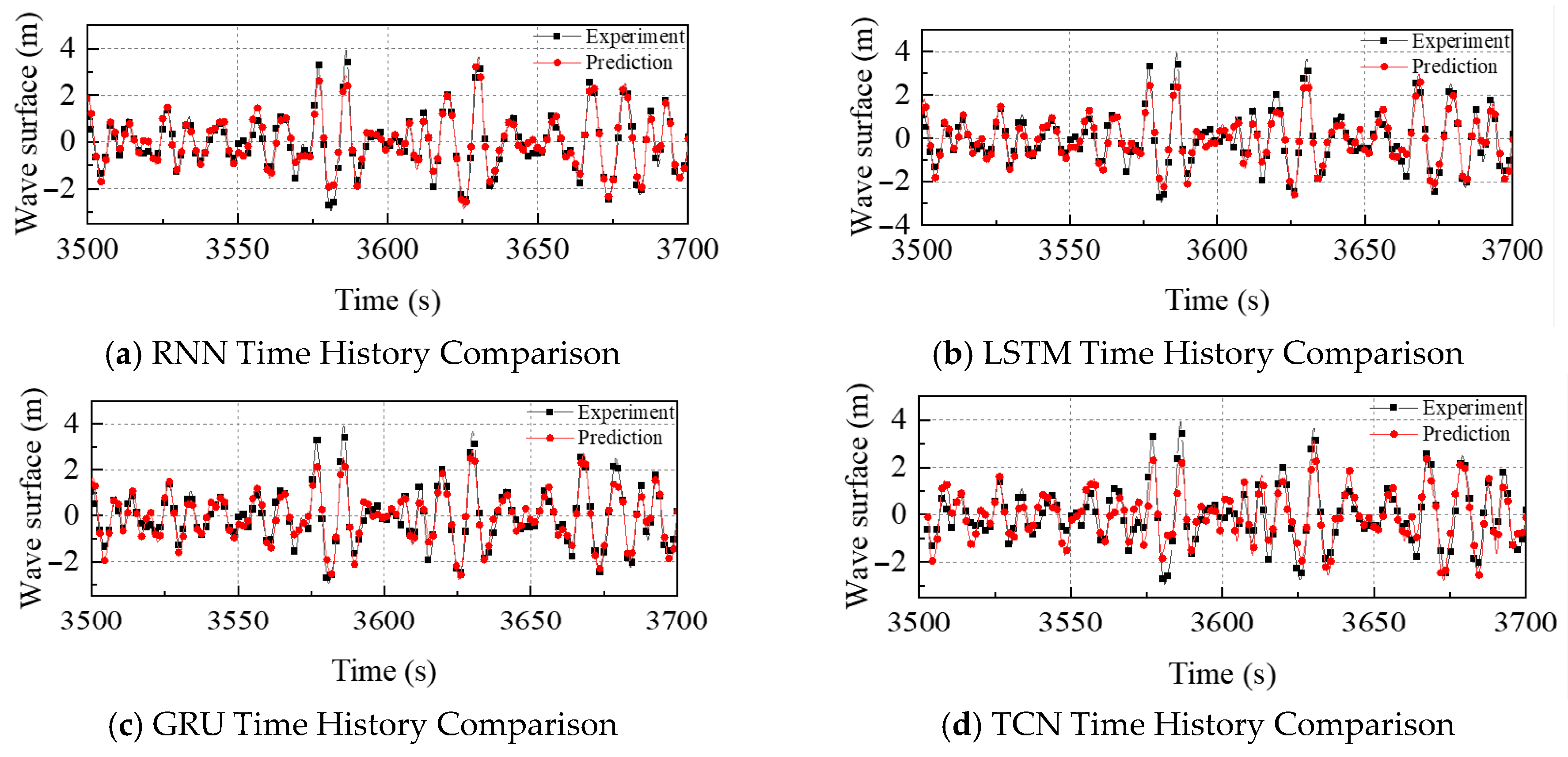
Under Sea-State 4, all four models accurately reproduce the temporal evolution of free-surface elevation, capturing both wave amplitude and phase with high fidelity. As depicted in Figure 8, the models exhibit different error characteristics that directly explain their respective RMSE values. The RNN-WP variant (Figure 8a) demonstrates optimal performance in the high-frequency band, particularly during intervals 3545–3555 s and 3625–3650 s, but it exhibits a slight phase lag in the low-frequency components. These combined errors result in an RMSE of 0.28 m. The LSTM-WP model (Figure 8b), an enhanced recurrent architecture, exhibits slightly superior overall skill but shows localized performance degradation in the same high-frequency windows. This degradation, attributable to LSTM’s stronger temporal dependencies becoming detrimental at short wave periods, is a key contributor to its RMSE of 0.27 m. The GRU-WP model (Figure 8c) outperforms LSTM-WP in tracking high-frequency surface features but demonstrates systematic amplitude errors at low frequencies (e.g., 3580 s and 3600 s). These low-frequency amplitude inaccuracies are the primary reason for its higher total RMSE of 0.29 m. Finally, the TCN-WP model (Figure 8d) excels at low-frequency reconstruction, accurately tracking the dominant wave crests and troughs, but incurs significant phase and amplitude errors in the high-frequency range (e.g., around 3625–3650 s). Despite these localized high-frequency inaccuracies, its superior performance in the energy-dominant low-frequency band leads to the lowest overall RMSE of 0.21 m among all four models. The time history comparisons for all four models at Sea State 4 are shown in Figure 8.

When the sea state advances to Level 5, intensified wave nonlinearity elevates the root-mean-square error (RMSE) for all models, as shown in Table 3. Despite larger absolute errors, the four architectures demonstrate enhanced fidelity in amplitude and phase reconstruction, alongside improved feature extraction capabilities. As depicted in the time history comparisons in Figure 9, these visual improvements are directly linked to the models’ RMSE values. Specifically, all models capture high-amplitude events with greater precision, achieving accurate predictions for strongly nonlinear segments (e.g., 3580–3590 s and 3655–3670 s). The improved ability to predict these extreme events, which contribute significantly to the overall error, helps to moderate the RMSE increase despite the more challenging conditions. Phase prediction also shows improvement relative to Level 4; for instance, the models successfully recover high-frequency phase information (3670–3700 s) that was lost in the Level 4 simulations (Figure 7), leading to more accurate estimates in these regions. As sea state increases, the spectral peak shifts toward lower frequencies, tightening temporal correlations among wave components—this change enhances the models’ phase discrimination across complex frequency bands. Since the significant wave-height increment is smaller than the absolute error increment, the overall surface-height agreement improves, which is reflected in the RMSE values (e.g., 0.39 m for RNN-WP) being only moderately higher than those at Sea State 4. These observations are supported by the time history comparisons presented in Figure 9.

When the sea state reaches level 6, the absolute errors of all four models increase, consistent with observations at level 5; however, relative to level-5 predictions, the agreement between predicted and actual wave surfaces deteriorates, leading to higher RMSE values as reported in Table 3. The detailed time history comparisons in Figure 10 illustrate the specific nature of these errors. Specifically, the RNN-WP model (Figure 10a) exhibits a pronounced phase lag in the low-frequency band, a primary contributor to its RMSE of 0.43 m. The LSTM-WP model (Figure 10b) introduces significant phase errors in the high-frequency range (3590–3610 s), which are the main source of its equivalent RMSE of 0.43 m. The GRU-WP model (Figure 10c) predictions peaks that are phase-misaligned with measured counterparts (3570–3600 s), and these phase discrepancies, combined with other errors, result in a higher RMSE of 0.45 m. The TCN-WP model (Figure 10d) displays simultaneous variability in amplitude and phase, achieving acceptable fidelity in certain intervals (3660–3700 s) while exhibiting degradation in others (3620–3640 s). These inconsistencies in prediction accuracy across different time intervals are reflected in its RMSE of 0.37 m, which, while the lowest among the four models at this sea state, still represents a significant drop in performance compared to milder conditions. The detailed time history comparisons for Sea State 6 are illustrated in Figure 10.

These deficiencies are attributable to intensified nonlinear hydrodynamic interactions as sea state rises, particularly evident at large amplitudes and in regions of complex frequency content. Despite elevated and oscillatory prediction errors, the four models still accurately reproduce overall wave-surface undulations. Finally, at level 6 the errors of RNN-WP and LSTM-WP converge, indicating equivalent model performance under these severe conditions.

When sea state escalates to level 7, the prediction error increases to approximately 0.61 m, affecting all models to varying degrees; nevertheless, they still reproduce the temporal evolution of surface elevation with acceptable fidelity. Although the prediction errors of RNN-WP and LSTM-WP rise to 0.61 m and their agreement with observations deteriorates further, both models continue to provide accurate phase and amplitude estimates. At this stage, nonlinearities in surface elevation impede feature extraction, causing errors to propagate from regions of large amplitude and complex frequency content to quieter segments (e.g., 3630–3645 s). GRU-WP exhibits similar error growth (RMSE ≈ 0.51 m) driven by increased nonlinearity, with discrepancies migrating from high-amplitude, high-complexity regions toward calmer intervals (3570–3630 s). Yet, relative to RNN-WP and LSTM-WP, GRU-WP yields more accurate predictions; moreover, as the dominant energy band shifts toward lower frequencies, wave coherence increases and no discernible phase error appears at any location. TCN-WP attains an RMSE of 0.42 m; its correspondence with measured surface elevation declines relative to sea-state 6, and it exhibits slight phase drifts in selected low-frequency windows (3610–3620 s). Nonetheless, the model maintains a distinct advantage in capturing large wave amplitudes and continues to provide reliable phase and amplitude predictions overall. The performance of all models at Sea State 7 is visualized in the time history plots of Figure 11.

As illustrated in Figure 7, the prediction errors of all models increase monotonically with the sea state level, consistent with the heightened nonlinear dynamics of wave propagation under more severe conditions. Across all sea states, the TCN consistently exhibits lower prediction errors compared to recurrent architectures, suggesting comparatively superior predictive performance. Moreover, the rate of error growth in TCN remains modest across sea state levels, indicating enhanced robustness to nonlinear variability.

4.2. Influence of Directional Spectrum

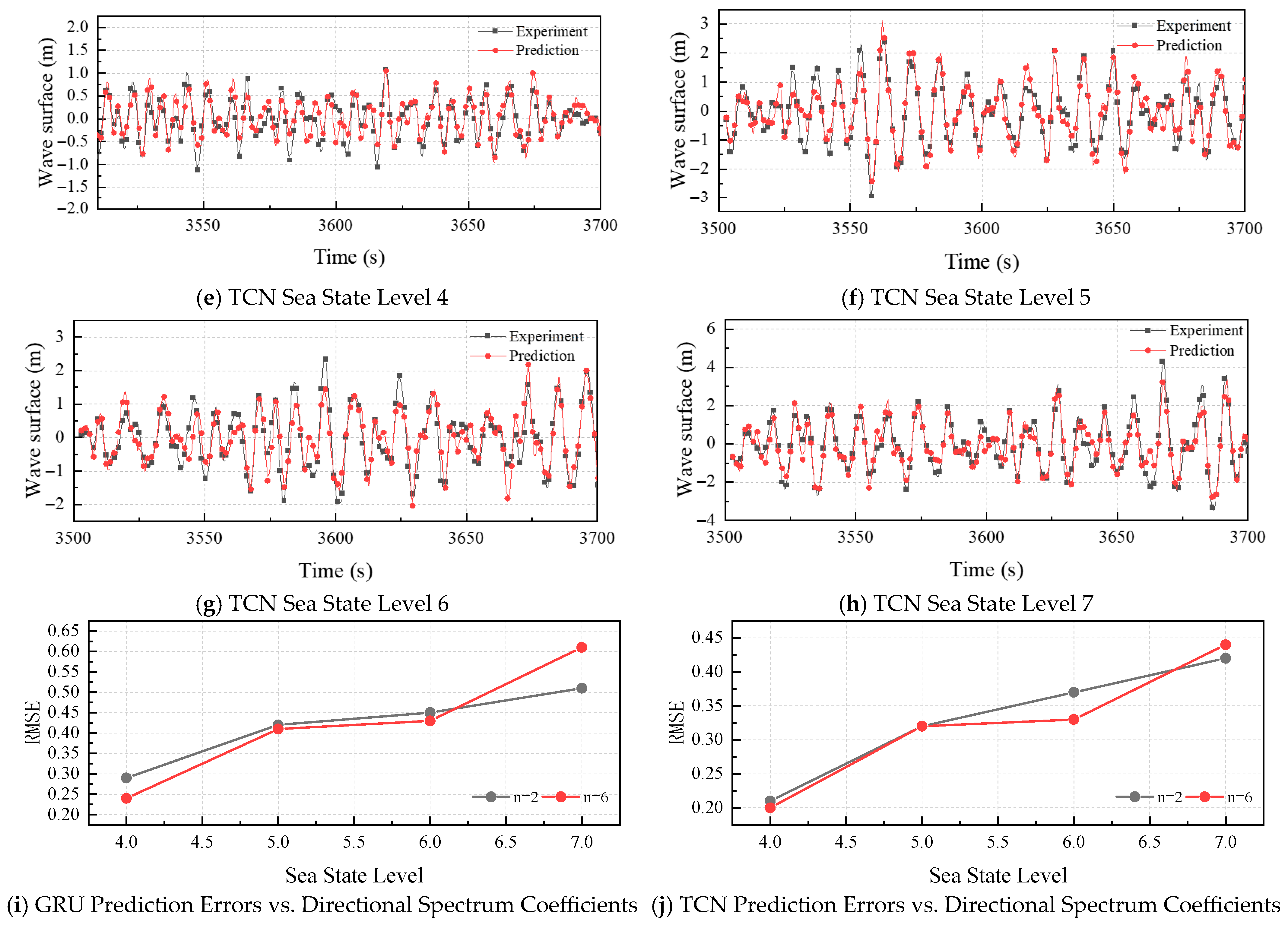
The directional spectrum constitutes an additional determinant of wave-field characteristics; any change in the spreading function directly modulates the cross-correlation between surface elevations at distinct spatial locations. Basin experiments employed two directional distributions. Predictions for a sea state with spreading parameter (n =2) were presented in the preceding subsection; here we analyze the complementary case (n = 6). The first 150 time steps recorded at gauges 1, 14, 15, 28, 29, 42, and 43 serve as input, with surface elevation at gauge 22 predicted 10 steps ahead.

Table 4. Quantitative Prediction Errors of the Four Models Across Four Sea-State Levels(n = 6).

	Model Names	RNN	LSTM	GRU	TCN
Sea State Levels
4		0.23	0.20	0.24	0.20
5		0.38	0.38	0.41	0.32
6		0.41	0.48	0.43	0.33
7		0.52	0.79	0.61	0.44

and Figure 12 list the prediction errors for sea states 4–7 generated by the four models.

To isolate the influence of the directional spectrum on prediction performance and to keep the analysis concise, we retain only the GRU model as the representative recurrent architecture and the TCN model, in accordance with the conclusions of the preceding subsection.

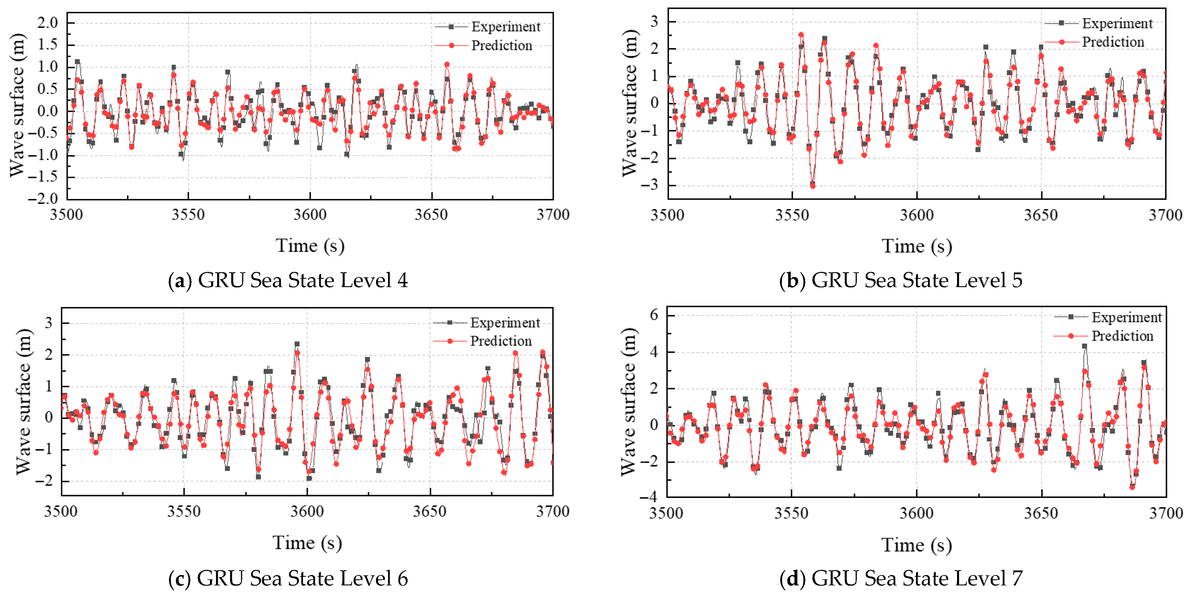
Analyses of TCN-WP and GRU-WP outputs are summarized below. The prediction errors for sea states 4–7 generated by the four models are listed in Table 4 and Figure 13. The detailed time history comparisons for GRU and TCN models under various sea states and directional spectra are presented in Figure 13. Figure 13a,e demonstrates that under sea-state 4 with directional spreading parameter n = 6, both models accurately reproduce surface elevation phase across most records; however, minor phase lags emerge in medium- and low-frequency bands, with systematic underestimation of certain large amplitudes. Nevertheless, RMSE remains lower than that obtained for n = 2.

As sea state escalates to levels 5 and 6, wave-surface predictions for n = 6 maintain qualitative similarity to those for n = 2. Figure 13b,c,f,g and Table 4 indicate comparable accuracy and absolute errors between the two spreading exponents, with overall satisfactory skill retention. At sea-state 7, performance for n = 6 deteriorates relative to n = 2.

The regulatory effect of directional spreading on model performance is significantly modulated by sea-state severity, validating the nonlinearity dominance conclusion from Section 4.1. In weakly nonlinear regimes (SS4–6), narrow spreading (n = 6) enhances spatial coherence by concentrating wave energy, paradoxically improving feature extraction. However, in strongly nonlinear regimes (SS7), the same concentration triggers directional amplification of wave–wave interactions, where sum/difference-frequency components accumulate along the dominant direction, causing prediction errors to surge dramatically. Thus, the impact of directional spreading is fundamentally sea-state-dependent: it optimizes feature learning under mild conditions but acts as a nonlinearity amplifier under severe conditions.

4.3. Influence of Prediction Distance

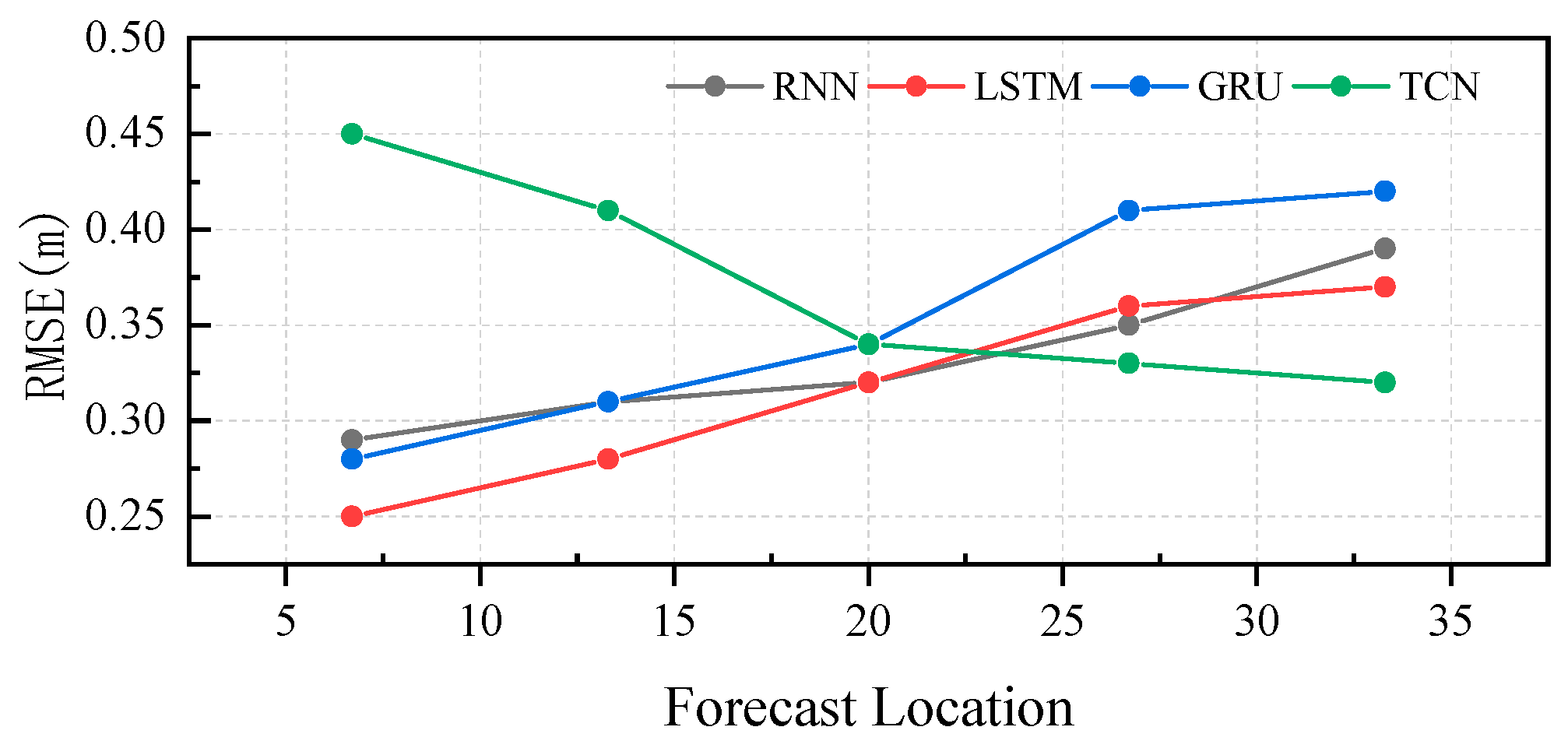
During spatial wave propagation, the cross-correlation between gauges diminishes with increasing prediction distance. This subsection quantifies the impact of prediction distance under fixed conditions: sea state 5 and directional spreading coefficient n = 2. Target locations are positioned at full-scale separations of 6.7 m (gauge 26), 13.3 m (gauge 25), 20 m (gauge 24), 26.7 m (gauge 23), and 33.3 m (gauge 22). Input data consist of the initial 150 time steps recorded at gauges 1, 14, 15, 28, 29, 42, and 43.

Table 5. Quantitative Prediction Error of Four Models Across Measurement Points.

	Model Names	RNN	LSTM	GRU	TCN
Prediction Location
22		0.39	0.37	0.42	0.32
23		0.35	0.36	0.41	0.33
24		0.32	0.32	0.34	0.34
25		0.31	0.28	0.31	0.41
26		0.29	0.25	0.28	0.45

summarizes the prediction errors for the four models at each downstream position (see Figure 14).

Examination of the error profiles indicates that the three recurrent architectures exhibit nearly identical distance dependence: RMSE increases monotonically with prediction distance, with the LSTM model demonstrating superior overall performance. Conversely, the one-dimensional temporal-convolution-based TCN displays the opposite trend—its RMSE diminishes as separation increases. To isolate the effect of prediction distance on prediction accuracy, we thus select LSTM and TCN as representative models for detailed analysis (see Figure 15).

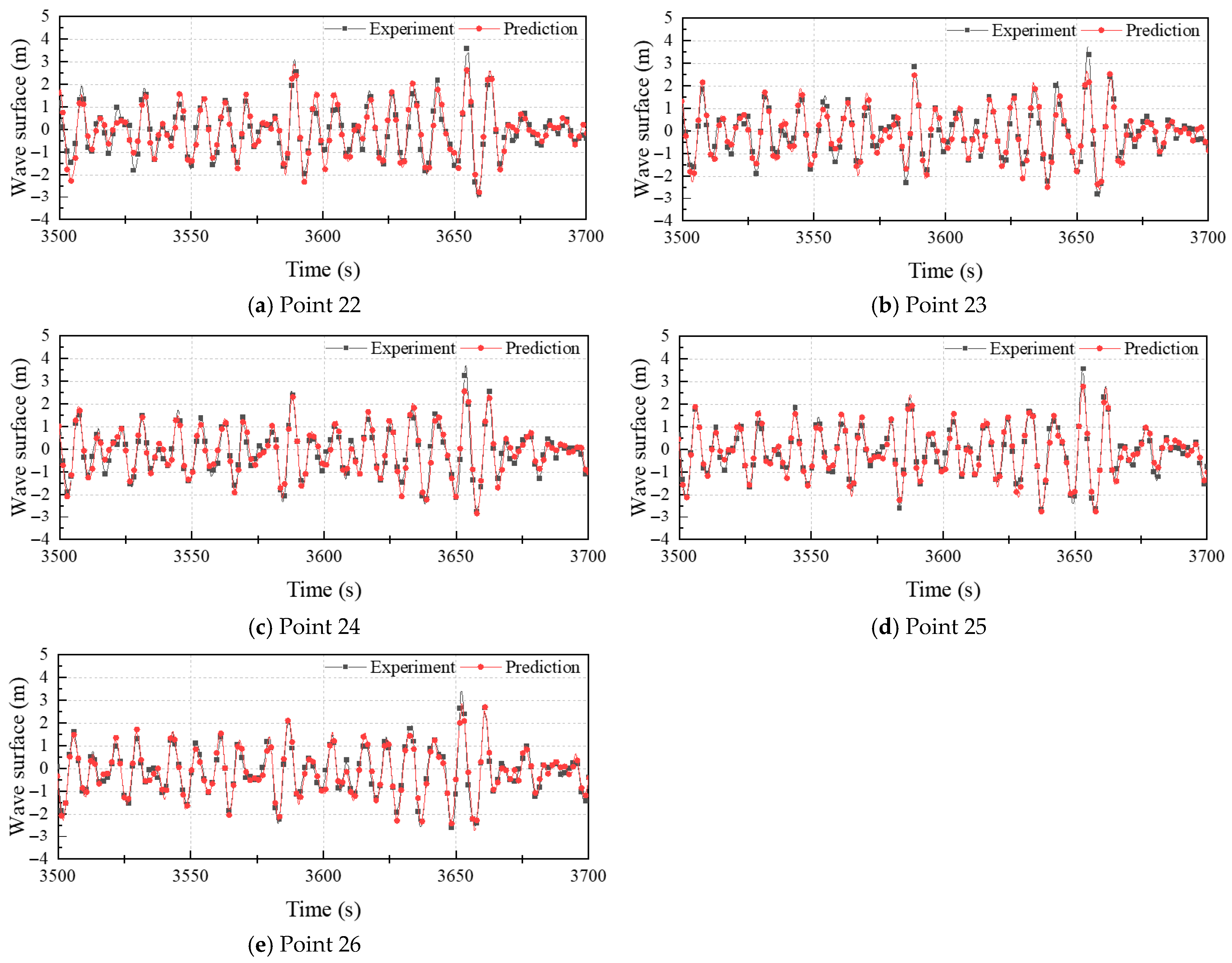
The prediction skill of the LSTM-WP model exhibits significant distance dependence. At a 33.3 m fetch, the model fails to resolve high-frequency excursions (e.g., t = 3523 s, 3528 s) while underestimating peak amplitudes (e.g., t = 3657 s), indicating diminished instantaneous fidelity. Reducing the fetch to 20 markedly refines high-frequency reconstruction: fine-scale, multi-frequency features (t = 3675 s, 3700 s) are now captured, and maxima align more closely with observations. At a 6.7 m fetch, the model resolves even rapid temporal fluctuations and accurately tracks extreme amplitudes, reducing overall RMSE to 0.25 m.

This behavior stems from wave evolution physics. Energy dissipation, nonlinear triad/quadruplet interactions, and frequency dispersion accumulate along the propagation path, introducing high-wavenumber–high-frequency content and increasing local complexity. Although LSTM’s gating mechanism excels at encoding long-range temporal dependencies, cumulative nonlinear distortions beyond ≈20 m exceed its effective memory horizon, degrading predictive accuracy.

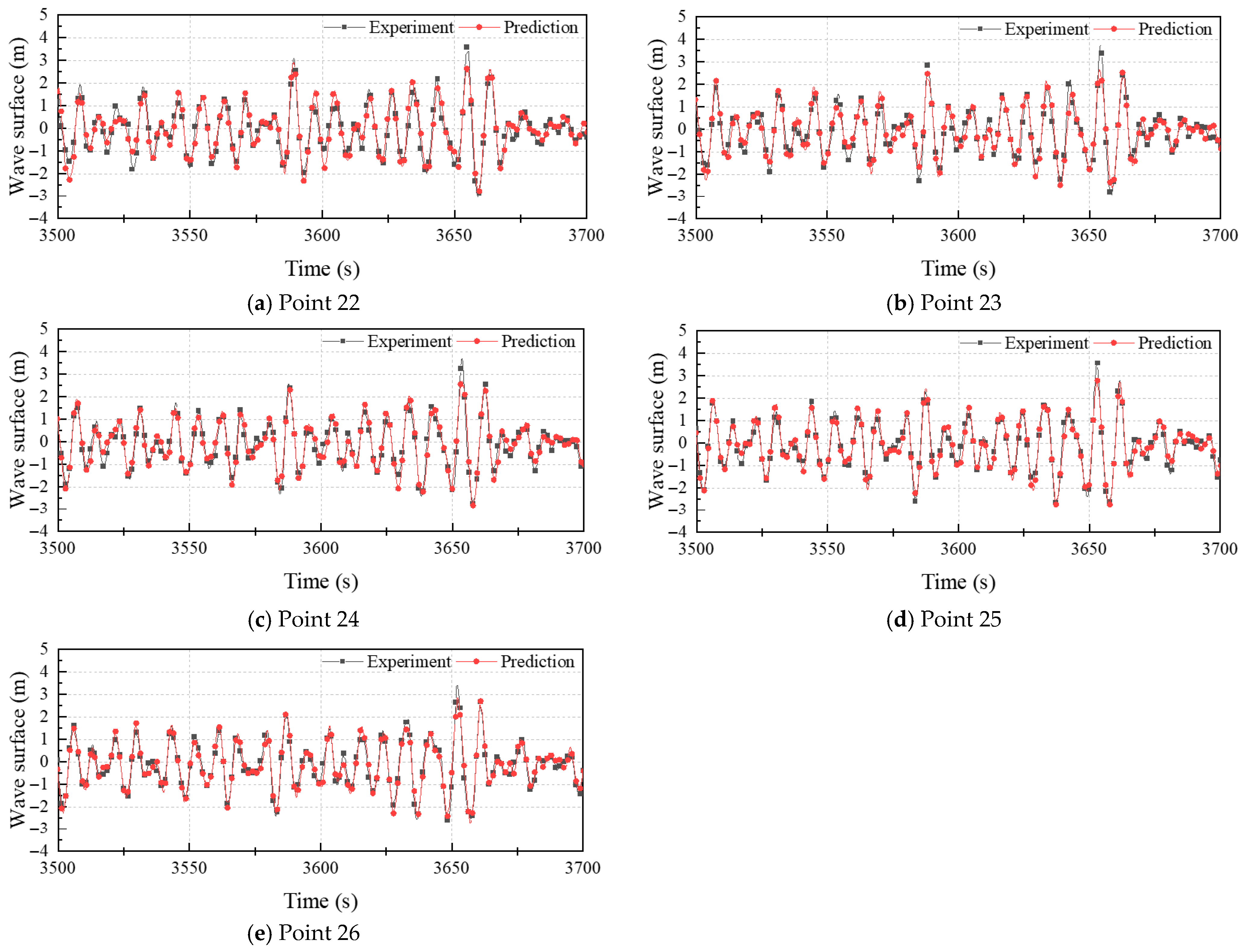
The TCN-WP model exhibits a counter-intuitive decline in accuracy as prediction distance decreases (Figure 16a–e). At 33.3 m fetch, reconstruction remains satisfactory except for slight under-prediction of specific large crests (e.g., t = 3620, 3630 s). When reduced to 20 m, the model fails to capture both high-frequency ripples and peak amplitudes, losing fine-scale structures within the rapidly varying surface. At the closest station (6.7 m), TCN-WP merely reproduces low-frequency trends, with amplitude and phase fidelity deteriorating significantly, resulting in an RMSE of 0.45 m.

This behavior stems from the interplay between TCN’s architectural bias and wave-field evolution. Causal dilated convolutions provide TCN with a wide receptive field that efficiently exploits spatial correlations, enabling superior performance when wave fields exhibit along-propagation coherence. Conversely, TCN’s kernel-based inductive bias offers limited frequency resolution, rendering it insensitive to high-wavenumber components that dominate near-generation regions under reflective boundary conditions. As fetch shortens, these locally generated broadband features exceed the model’s representational capacity. Additionally, wave evolution shifts from a spatial-correlation-dominated regime (where TCN excels) to a time-continuity-dominated regime favoring autoregressive architectures, further exacerbating TCN’s performance degradation at close range.

Prediction distance differentially impacts model performance through a spatial evolution mechanism, revealing fundamental conflicts between wave propagation physics and model architectures. For recurrent models (RNN/LSTM/GRU), RMSE increases monotonically with distance. This is due to the cumulative complex disturbances during wave propagation, which gradually exceed the memory limit of the recurrent models. Conversely, the convolutional TCN excels at long distances by leveraging dilated convolutions’ large receptive field to exploit spatial correlations and smooth high-frequency disturbances. However, its performance degrades sharply at short ranges (<15 m) because the dominant mechanism shifts from spatial-correlation-dominated regimes to time-continuity-dominated regimes, whereas the TCN model is better suited for the spatial-correlation-dominated regime. Thus, the impact of prediction distance is fundamentally a model-physics matching problem: TCN should be prioritized for long-range predictions, while recurrent models are superior for short-range forecasts.

4.4. Influence of Prediction Lead Time

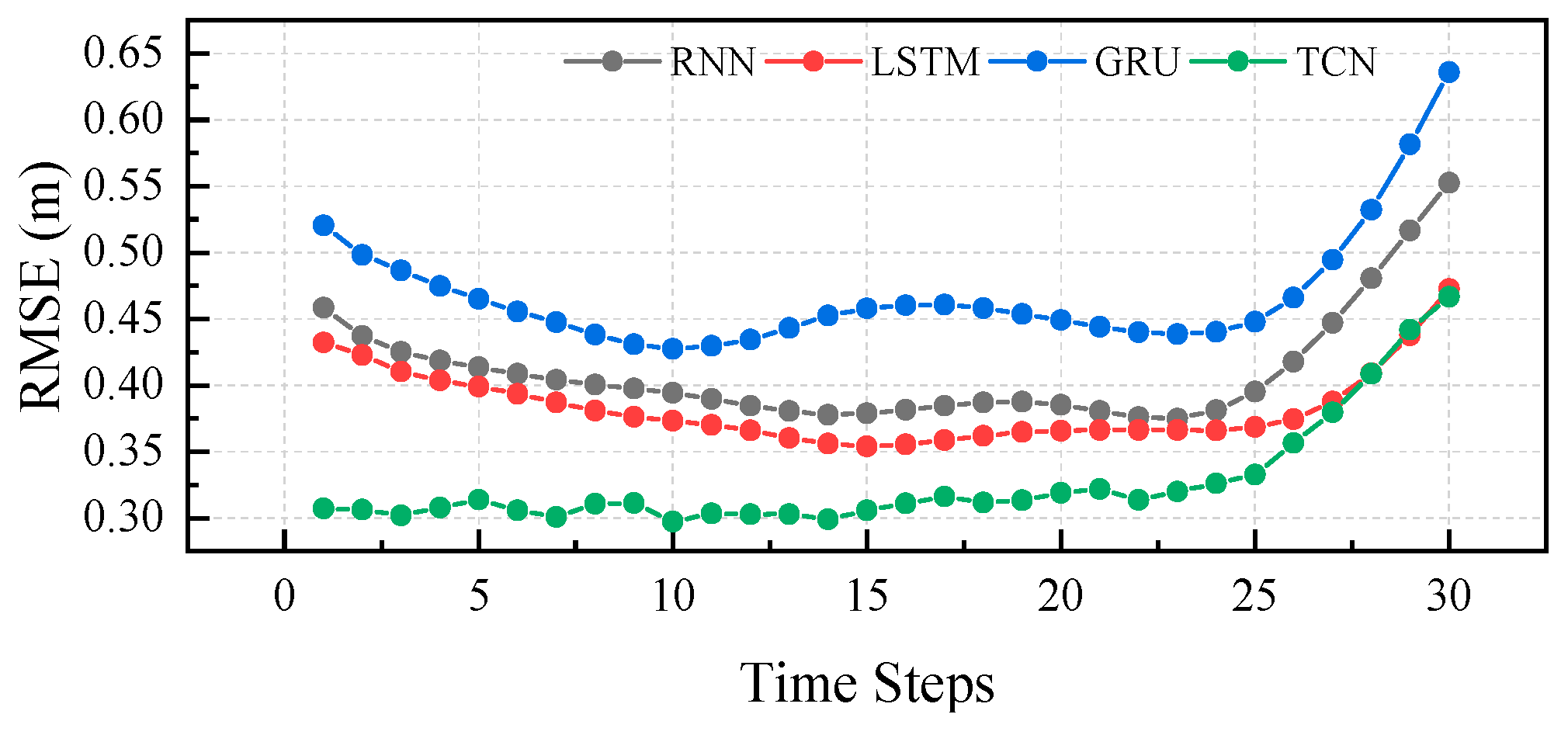
Beyond spatial heterogeneity, wave processes exhibit significant temporal decorrelation. To quantify the impact of prediction horizon on accuracy, we maintain sea state at level 5 and directional spreading coefficient at n = 2. The initial 150 time steps from gauges 1, 14, 15, 28, 29, 42, and 43 serve as input to predict surface elevation at gauge 22 over a 30-step horizon. Figure 17 summarizes the RMSE values for all four models under this configuration.

The temporal-decay signature is nearly identical for the three recurrent architectures—RNN-WP, LSTM-WP, and GRU-WP—differing only in absolute magnitude, and can be characterized as a single continuum naturally divided into three intervals. In the first interval (lead steps 1–10), LSTM-WP error decreases while TCN error remains low and nearly flat; this occurs because ultra-short prediction horizons force the 150-step input window to contain early surface fluctuations that have lost dynamical relevance to the immediate future. For LSTM-WP, these “obsolete memories” pass through recurrent gates and momentarily act as noise inflating initial RMSE, whereas TCN—whose receptive field is rigidly defined by stacked dilated causal kernels—inherently excludes irrelevant lags, yielding cleaner ultra-short-range predictions. When the horizon enters the second interval (steps 11–25), the input sequence optimally overlaps with the wave group reaching the target location after one persistence time; information content aligns optimally with the future state, causing both model families to settle into an essentially constant error plateau. Beyond this lies the third interval (steps 26–30), where temporal separation exceeds the coherence lifetime of dominant wave components: dispersive spreading, nonlinear triad energy redistribution, and residual stochastic forcing progressively alter the surface, monotonically weakening the statistical coupling between encoded history and forthcoming elevation. Consequently, regardless of whether the model employs gated recurrence or temporal convolution, its RMSE exhibits a steady increase throughout the 30-step prediction window.

This temporal-decay pattern, as evidenced by the error evolution in Figure 17, reveals a fundamental deterministic predictability limit shared by all architectures: when lead time exceeds the wave group’s coherence time, statistical coupling between historical and future states inevitably deteriorates. The divergence between recurrent and convolutional models in ultra-short horizons further exposes critical architectural biases—recurrent models suffer from ‘obsolete memory’ contamination due to their sequential information processing, while TCN’s receptive field provides inherent noise immunity. Both TCN and recurrent models exhibit a degree of stability in intermediate predictions (steps 11–25).

5. Conclusions

This study systematically evaluates the performance of four deep learning models in phase-resolved wave prediction, with particular attention to how sea state severity, directional spreading, prediction distance, and lead time modulate accuracy. Across all models, increasing sea state severity introduces nonlinear wave characteristics that degrade predictive fidelity, with recurrent architectures (RNN, LSTM, GRU) showing sharper error escalation under strong nonlinearity, while TCN maintains relative robustness by exploiting spatial correlations, albeit at the cost of high-frequency fidelity. Directional spectrum enhances model performance under mild conditions by improving spatial coherence, but amplifies errors in severe sea states by intensifying directional wave–wave interactions. The analysis of forecast distance clarifies the performance disparity between the models: recurrent models rely on temporal continuity to maintain short-range accuracy but deteriorate in long-range predictions; in contrast, the TCN excels in long-range forecasting due to its receptive field structure, underperforming only at close range where local broadband features dominate. Similarly, lead time effects expose a temporal predictability limit shared by all architectures, with recurrent models vulnerable to memory contamination in ultra-short horizons and TCN offering more stable intermediate-range predictions. Collectively, these findings highlight that model performance is context-dependent, requiring the alignment of architectural strengths with the dominant physical mechanisms whether nonlinear, directional, spatial, or temporal characterizing the wave field under consideration.

In conclusion, this study confirms that deep-learning models can deliver accurate phase-resolved wave forecasts and clarifies how sea state, directional spreading, prediction distance and lead time control their skill. However, it is important to acknowledge the study’s limitations. The present research is restricted to four mainstream architectures (RNN, LSTM, GRU, and TCN); more recent options such as attention-based models or graph neural networks have not been examined. In addition, all conclusions are drawn from a single wave-basin dataset, whereas real seas exhibit far greater variability in spectrum shape, site geography, and seasonal climate. Therefore, the proposed selection guidelines should be viewed as an initial rather than universal reference. Future work should (i) test additional architectures and hybrid designs, and (ii) validate these findings with field measurements or high-fidelity numerical simulations to improve generalization.

References

1. Kourafalou, V.; De Mey, P.; Staneva, J.; Ayoub, N.; Barth, A.; Chao, Y.; Cirano, M.; Fiechter, J.; Herzfeld, M.; Kurapov, A.; et al. Coastal Ocean Forecasting: Science foundation and user benefits. J. Oper. Oceanogr. 2015, 8 (Supp. 1), s147–s167. [Google Scholar] [CrossRef]
2. Makris, C.; Papadimitriou, A.; Baltikas, V.; Spiliopoulos, G.; Kontos, Y.; Metallinos, A.; Androulidakis, Y.; Chondros, M.; Klonaris, G.; Malliouri, D.; et al. Validation and Application of the Accu-Waves Operational Platform for Wave Forecasts at Ports. J. Mar. Sci. Eng. 2024, 12, 220. [Google Scholar] [CrossRef]
3. Ravdas, M.; Zacharioudaki, A.; Korres, G. Implementation and validation of a new operational wave forecasting system of the Mediterranean Monitoring and Forecasting Centre in the framework of the Copernicus Marine Environment Monitoring Service. Nat. Hazards Earth Syst. Sci. 2018, 18, 2675–2695. [Google Scholar] [CrossRef]
4. Kerczek, C.V.; Davis, S.H. Linear stability theory of oscillatory Stokes layers. J. Fluid Mech. 1974, 62, 753–773. [Google Scholar] [CrossRef]
5. Dalzell, J.F. A note on finite depth second-order wave–wave interactions. Appl. Ocean Res. 1999, 21, 105–111. [Google Scholar] [CrossRef]
6. Wang, G.; Pan, Y. Data Assimilation for Phase-Resolved Ocean Wave Forecast. In Proceedings of the ASME 2020 39th International Conference on Ocean, Offshore and Arctic Engineering, Virtual Online, 3–7 August 2020; ASME: New York, NY, USA, 2020; Volume 6B, p. V06BT06A071. [Google Scholar] [CrossRef]
7. Yao, J.; Zhang, X. Deterministic reconstruction and prediction model of multi-level nonlinear wave fields. In Proceedings of the 16th National Conference on Hydrodynamics & 32nd National Symposium on Hydrodynamics, Wuxi, China, 30 October 2021; Volume II, pp. 831–841. (In Chinese). [Google Scholar]
8. Mohapatra, S.C.; Amouzadrad, P.; Bispo, I.B.S.; Guedes Soares, C. Hydrodynamic response to current and wind on a large floating interconnected structure. J. Mar. Sci. Eng. 2025, 13, 63. [Google Scholar] [CrossRef]
9. Schäffer, H.A.; Madsen, P.A.; Deigaard, R. A Boussinesq model for waves breaking in shallow water. Coast. Eng. 1993, 20, 185–202. [Google Scholar] [CrossRef]
10. Zhao, B. Numerical Simulation Methods for Three-Dimensional Nonlinear Water Waves Based on G-N Theory. Ph.D. Thesis, Harbin Engineering University, Harbin, China, 2010. (In Chinese). [Google Scholar]
11. Stuhlmeier, R.; Stiassnie, M. Deterministic wave forecasting with the Zakharov equation. J. Fluid Mech. 2021, 913, A50. [Google Scholar] [CrossRef]
12. Lange, H. On Dysthe’s nonlinear Schrödinger equation for deep water waves. Transp. Theory Stat. Phys. 2000, 29, 509–524. [Google Scholar] [CrossRef]
13. Aziz, T.M. Statistics of nonlinear wave crests and groups. Ocean Eng. 2006, 33, 1589–1622. [Google Scholar] [CrossRef]
14. Tsai, P.-H.; Fischer, P.; Iliescu, T. A time-relaxation reduced order model for the turbulent channel flow. J. Comput. Phys. 2025, 521 Pt 1, 113563. [Google Scholar] [CrossRef]
15. Schmidhuber, J. Deep learning in neural networks: An overview. Neural Netw. 2015, 61, 85–117. [Google Scholar] [CrossRef]
16. Zhang, Q.; Zhang, H.; Zhao, X.; Ding, J.; Xu, D. Multiple-input operator network prediction method for nonlinear wave energy converter. Ocean Eng. 2025, 317, 120106. [Google Scholar] [CrossRef]
17. Quang, T.L.; Dao, M.; Lu, X. Prediction of near-field uni-directional and multi-directional random waves from far-field measurements with artificial neural networks. Ocean Eng. 2023, 278, 114307. [Google Scholar] [CrossRef]
18. Ma, X.; Duan, W.; Huang, L.; Qin, Y.; Yin, H. Phase-resolved wave prediction for short crest wave fields using deep learning. Ocean Eng. 2022, 262, 112170. [Google Scholar] [CrossRef]
19. Zhang, J.; Zhao, X.; Jin, S.; Greaves, D. Phase-resolved real-time ocean wave prediction with quantified uncertainty based on variational Bayesian machine learning. Appl. Energy 2022, 324, 119711. [Google Scholar] [CrossRef]
20. Wedler, M.; Stender, M.; Klein, M.; Hoffmann, N. Machine learning simulation of one-dimensional deterministic water wave propagation. Ocean Eng. 2023, 284, 115222. [Google Scholar] [CrossRef]
21. Zhao, Y.; Su, D.; Zou, L.; Wang, A. Freak wave prediction based on LSTM neural networks. J. Huazhong Univ. Sci. Tech. 2020, 48, 47–51. (In Chinese) [Google Scholar]
22. Kim, Y.; Ha, Y.; Choi, J. Preliminary study on wave height prediction with convolutional neural network. In Proceedings of the Thirty-first (2021) International Ocean and Polar Engineering Conference, Corfu, Greece, 20–25 June 2021; International Society of Offshore and Polar Engineers: Reston, VA, USA, 2021; p. I–21–3133. [Google Scholar]
23. Yu, S. Ocean Wave Simulation and Prediction. Ph.D. Thesis, Virginia Polytechnic Institute and State University, Blacksburg, VA, USA, 2018. [Google Scholar]
24. Duan, W.; Ma, X.; Huang, L.; Liu, Y.; Duan, S. Phase-resolved wave prediction model for long-crest waves based on machine learning. Computer. Methods Appl. Mech. Eng. 2020, 372, 113350. [Google Scholar] [CrossRef]
25. Law, Y.Z.; Santo, H.; Lim, K.Y.; Chan, E.S. Deterministic wave prediction for unidirectional sea-states in real-time using artificial neural network. Ocean Eng. 2020, 195, 106722. [Google Scholar] [CrossRef]
26. Liu, Y.; Zhang, X.; Dong, Q.; Chen, G.; Li, X. Phase-resolved wave prediction with linear wave theory and physics-informed neural networks. Appl. Energy 2024, 355, 121602. [Google Scholar] [CrossRef]
27. Ehlers, S.; Klein, M.; Heinlein, A.; Wedler, M.; Desmars, N.; Hoffmann, N.; Stender, M. Machine learning for phase-resolved reconstruction of nonlinear ocean wave surface elevations from sparse remote sensing data. Ocean Eng. 2023, 288, 116059. [Google Scholar] [CrossRef]
28. Agyekum, E.B.; PraveenKumar, S.; Eliseev, A.; Velkin, V.I. Design and construction of a novel simple and low-cost test bench point-absorber wave energy converter emulator system. Inventions 2021, 6, 20. [Google Scholar] [CrossRef]
29. WMO. WMO Sea-Ice Nomenclature; WMO-No. 558; World Meteorological Organization: Geneva, Switzerland, 2018; ISBN 978-92-63-10558-5. [Google Scholar]
30. Faltinsen, O.M. Sea Loads on Ships and Offshore Structures, Chinese ed.; Yang, J.; Xiao, L.; Ge, C., Translators; Shanghai Jiao Tong University Press: Shanghai, China, 2008; ISBN 978-7-313-03029-9. [Google Scholar]
31. Belmont, M.R.; Horwood, J.M.K.; Thurley, R.W.F.; Baker, J. Filters for linear sea-wave prediction. Ocean Eng. 2006, 33, 2332–2351. [Google Scholar] [CrossRef]
32. Elman, J.L. Finding structure in time. Cogn. Sci. 1990, 14, 179–211. [Google Scholar] [CrossRef]
33. Sepp Hochreiter, Jürgen Schmidhuber; Long short-term memory. Neural Comput. 1997, 9, 1735–1780. [CrossRef]
34. Chung, J.; Gülçehre, Ç.; Cho, K.; Bengio, Y. Empirical evaluation of gated recurrent neural networks on sequence modeling. arXiv 2014, arXiv:1412.3555. [Google Scholar] [CrossRef]
35. Bai, S.; Kolter, J.Z.; Koltun, V. An empirical evaluation of generic convolutional and recurrent networks for sequence modeling. arXiv 2018, arXiv:1803.01271. [Google Scholar] [CrossRef]
Figure 1. Experimental setup. (a) Layout of the wave basin (left) and photograph of the installed wave maker (right). The wave maker length is drawn and photographed at the same scale in both panels (physical length = 5 m). (b) Wave Gauge Array. (c) Wave Experiment.
Jmse 13 02196 g001
Figure 2. Schematic of wave propagation (1#–n#: fixed wave height measuring points).
Jmse 13 02196 g002
Figure 3. Schematic diagram of RNN neuron and architecture. (a) Structure of a single RNN neuron. (b) Unrolling of RNN over time steps.
Jmse 13 02196 g003
Figure 4. Schematic Diagram of LSTM Structure.
Jmse 13 02196 g004
Figure 5. Schematic Diagram of GRU Structure.
Jmse 13 02196 g005
Figure 6. Schematic Diagram of TCN Structure (a) the basic structure of the TCN, and (b) the detailed structure of the residual block.
Jmse 13 02196 g006
Figure 7. Evolution of Predictive Errors for the Four Models Across Four Sea-State Levels.
Jmse 13 02196 g007
Figure 8. Time History Comparison of Four Models at Sea State 4.
Jmse 13 02196 g008aJmse 13 02196 g008b
Figure 9. Time History Comparison of Four Models at Sea State 5.
Jmse 13 02196 g009
Figure 10. Time History Comparison of Four Models at Sea State 6.
Jmse 13 02196 g010
Figure 11. Time History Comparison of Four Models at Sea State 7.
Jmse 13 02196 g011
Figure 12. Evolution of Predictive Errors for the Four Models Across Four Sea-State Levels (n = 6).
Jmse 13 02196 g012
Figure 13. Time History Comparison of GRU/TCN under Multi-Sea States and Directional Spectra.
Jmse 13 02196 g013aJmse 13 02196 g013b
Figure 14. Evolution of Prediction Error of Four Models Across Measurement Points.
Jmse 13 02196 g014
Figure 15. LSTM Time History Comparison Diagrams at Different Measurement Points.
Jmse 13 02196 g015
Figure 16. TCN Time History Comparison Diagrams at Different Measurement Points.
Jmse 13 02196 g016
Figure 17. Effect of Time Step Size on Prediction Accuracy.
Jmse 13 02196 g017