Investigating Impacts of Risk Influence Factors on the Consequences of Marine Accidents in China by SE-CNN-GRU Algorithm

Abstract

Marine shipping safety is of great concern to many stakeholders, especially maritime authorities, and the consequences of marine accidents, linked to the accident severity and type, are intrinsically impacted by various risk influence factors (RIFs). To investigate the impacts of RIFs on marine accidents and the consequences thereof within Chinese waters, in this study, 1106 marine accident investigation reports issued by China’s MSA during the 2013–2024 period were collected, and a database of marine shipping RIFs was developed based on these data. As a result, 14 typical features were extracted, and the accident severity level and accident type were set as the output features. Then, a comprehensive machine learning algorithm integrating squeeze-and-excitation (SE), a convolutional neural network (CNN), and a gated recurrent unit (GRU) was proposed to process the extracted marine RIFs. Finally, these features were analyzed in terms of importance, correlation, and partial dependence plots (PDPs), and the performance of the SE-CNN-GRU algorithm, especially the prediction accuracy, was verified. The findings and results obtained from this study are valuable for improving shipping safety in Chinese waters; managerial implications are additionally proposed.

1. Introduction

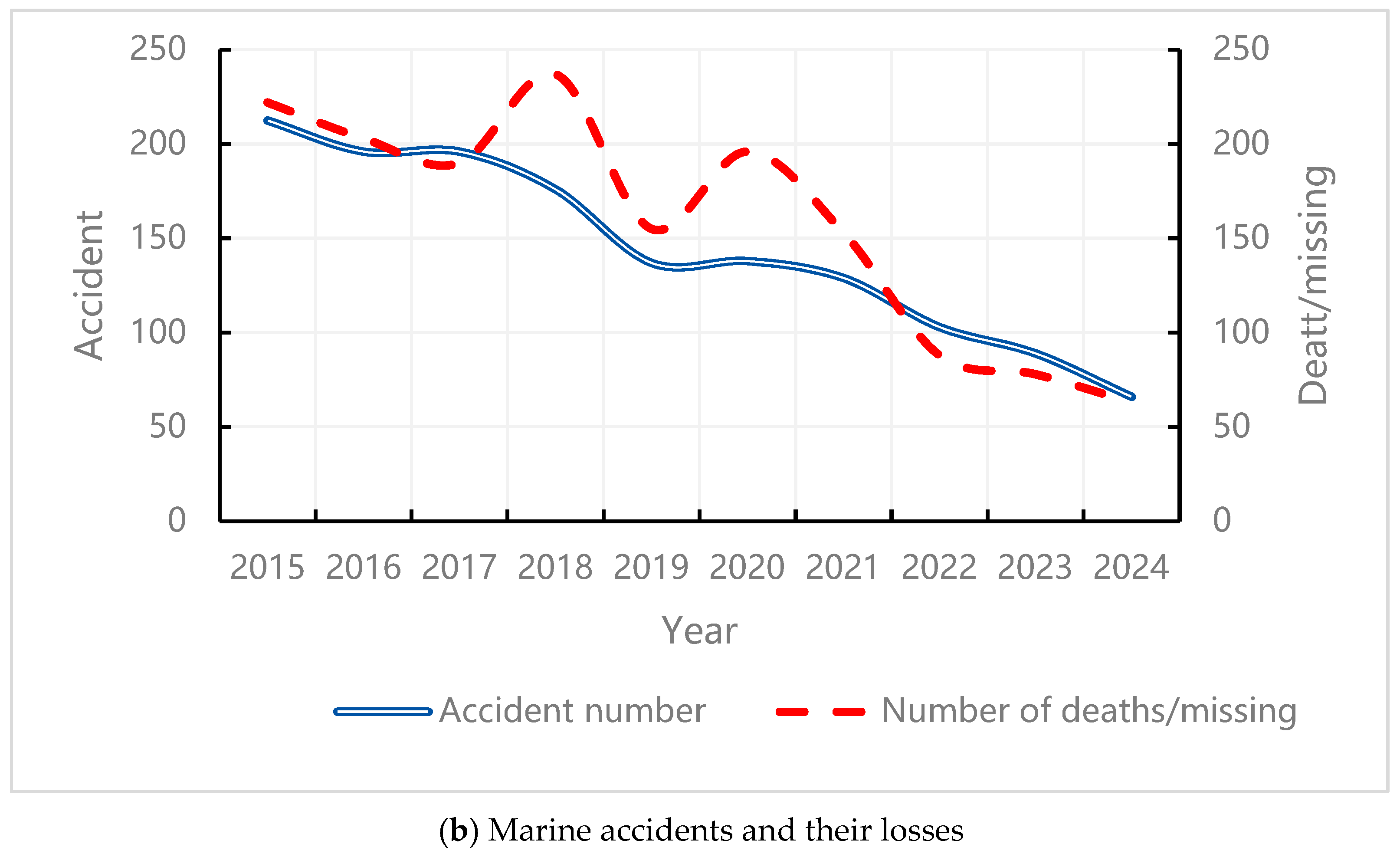
Water transportation is critical for the development of society and economy, especially in the People’s Republic of China. Using statistics issued by the Ministry of Transport of the People’s Republic of China, waterborne transportation volumes from the last decade (2015–2024) are presented in Figure 1a. It can clearly be seen that there was a continuous increase from 2015 to 2024. In addition, losses of life and property caused by marine accidents are consistently considered by authorities at different levels. For instance, the International Maritime Organization (IMO) works continuously to improve various maritime regulations and codes to guarantee shipping safety, and national maritime authorities and ship survey administrations work to improve ship technical levels [1]. The number of marine accidents has decreased in recent years, as have the losses caused by these accidents. For example, as shown in Figure 1b, in China, the number of marine accidents with at least one person dead/missing decreased from 203 in 2015 to 66 in 2024, and the number of deaths/missing individuals also decreased from 222 to 63 in the same time span. However, the safety of marine shipping is still not satisfactory as far as society and the general public are concerned [1], as marine accidents with high levels of social attention and huge losses still occasionally occur, such as the M/T SANCHI [2], ocean pollution [3], and fire/explosion accidents [4]. Therefore, investigating the potential patterns behind these marine accidents is an ongoing topic, and related outcomes are continuously used by decision-makers as valuable references for formulating and revising maritime regulations.

It is widely accepted that investigating the risk influence factors (RIFs) involved in marine accidents is an effective way to prevent similar accidents from occurring again [5]. Therefore, many scholars and decision-makers over many decades have dedicated themselves to collecting and analyzing the RIFs associated with marine accidents utilizing different technologies. Recently, the emergence of big data-related technologies, such as data mining, content analysis, machine learning, neural networks, and, in particular, various machine learning algorithms, has greatly improved efforts in this field, and these are regarded as effective technical tools in the field of RIF research.

In this study, we aim to explore the influence of RIFs on the consequences of marine accidents within Chinese waters by means of a machine learning algorithm. As is well known, the volume and quality of a dataset are crucial for machine learning algorithm operation and performance. Therefore, 1106 marine accident investigation reports issued by China’s MSA from 2013 to 2024 were collected for this study, and these were used to extract RIFs as the data features. As a result, a total of 14 features were obtained from these accident investigation reports. Subsequently, we proposed the comprehensive machine learning algorithm SE-CNN-GRU, which integrates a CNN, an SE module, and a GRU algorithm. The extracted data features were subsequently considered as the input of this proposed comprehensive machine learning algorithm, and as a result, the prediction performance of the SE-CNN-GRU algorithm was verified, and the data features obtained from the database were evaluated. The results of these experiments are used to discuss methods to improve the safety of shipping activities within Chinese waters. In addition, the potential applications of this comprehensive machine learning algorithm are also discussed in this paper.

The novel contributions of this study are summarized as follows.

(1)

A database of 1106 marine accidents that occurred within Chinese waters during the 2013–2024 period is established, and RIF data features were extracted as a dataset for the purpose of training machine learning algorithms.

(2)

A comprehensive machine learning algorithm (SE-CNN-GRU algorithm) aimed at exploring the influence mechanism of RIFs on marine accidents and the consequences thereof within Chinese waters is proposed. The proposed comprehensive machine learning algorithm is superior to more common machine learning algorithms, such as SVM, RF, and XGBoost, as verified in this study. The competitiveness of this comprehensive machine learning method may lie in its excellent performance in extracting feature information and in convolutional classification, as well as the combination of genetic algorithm features.

(3)

Some insights based on the results of the proposed machine learning algorithm are proposed in this study, which can be used to promote the safety of the shipping industry in China; in addition, potential applications of the proposed machine learning algorithm are also discussed.

The rest of this paper is organized as follows. Various studies on marine RIFs are reviewed and summarized in Section 2, and in Section 3, material preparation and the proposed machine learning algorithm are described in detail. In Section 4, the results obtained from the proposed machine learning algorithm are analyzed, and the prediction performance of this machine learning algorithm is verified. Finally, the results are discussed and the insights obtained from this study are proposed in Section 5.

2. Literature Review

2.1. Studies on the RIFs Involved in Marine Accidents

It is widely accepted by scholars that RIFs play an important role in preventing and predicting marine accidents. In addition, marine authorities and decision-makers manage and control various RIFs in the shipping industry to prevent accidents. According to Ragnar Rosness [6], a risk influencing factor is defined as “a set of conditions which influence the level of specified risks related to a given activity or system”, in which a “condition” refers to a relatively stable property of a system or its environment. Sometimes, RIFs are considered the potential causes of human errors and violations. Deng et al. [7] identified key RIFs by means of a complex network analysis using a collection of coastal marine accidents in China. Some studies have examined marine RIFs in more depth: Yu et al. [8] identified marine RIFs in terms of the crew, ship factors, human factors, and external environment factors based on a collection of marine occupational accidents, and similar research was also carried out by Feng et al. [9]. In practice, marine RIFs vary for different ship types; thus, Cao et al. [10] investigated the differences in RIFs for different types of vessels involved in accidents. In addition, marine RIFs may be considered as influencing factors for specific marine operations. RIFs for emergency operations in floating storage and regasification units were identified and assessed by Xiao et al. [11], and marine RIFs for navigational accidents within ice-covered waters were also investigated by Fu et al. [12].

Generally, marine RIFs are extracted from various marine accident databases; for example, Jiang et al. [13] utilized the global marine accident database created by Lloyd’s List Intelligence, which contains 55,469 marine accidents from January 2002 to October 2022. Similarly, the marine accidents recorded in the global integrated shipping information system (GISIS) maintained by the IMO are frequently used by scholars to investigate marine RIFs; Li et al. [14] utilized accident records from the GISIS from 2017 to 2021 to quantitatively analyze the marine RIFs affecting the occurrence of marine accidents. Marine accident records from the Marine Accident Investigation Branch (MAIB) and Transportation Safety Board (TSB) were collected by Cao et al. [15] to analyze the RIFs involved in 21,206 marine accidents. In addition, AIS data were also utilized by Dugan and Utne [16] to improve the identification of marine RIFs.

When it comes to the investigation or assessment of marine RIFs, various technologies have been applied by scholars. The Bayesian network (BN) is accepted as an effective tool for analyzing marine RIFs and was applied by Yin et al. [17] to study the association between marine RIFs and accident severity. Moreover, a data-driven BN was proposed by Cao et al. [18] to investigate the factors affecting the severity of marine accidents. Recently, a tree-augmented naive BN (TAN-BN) was used by Yu et al. [8] to explore the factors influencing occupational marine accidents. Similar studies on this topic that utilize BNs include those by Jiang et al. [13], Li et al. [14], Wang et al. [19], and Kammal and Cakir [20]. Complex network (CN)-based methodologies are also frequently used to analyze marine RIFs; for instance, Cao et al. [10] integrated a weighted influence non-linear gauge system (WINGS) and an adversarial interpretive structure model (AISM) based on a CN to study marine RIFs related to bulk carriers, container ships, fishing vessels, and oil tankers. The combination of a CN and association rule mining (ARM) was also proposed by Cao et al. [15] to analyze marine RIFs. Similarly, Wang et al. [21] utilized the WINGS, enhanced multilevel ARM, total adversarial Hasse diagram technology (TAHDT), and matrices impacts croises-multiplication appliance classement (MICMAC) to investigate the heterogeneous characteristics of marine RIFs. An ordered logistic regression model was developed by Wang et al. [22] to explore the relationship between the severity of marine accidents and RIFs. Recently, machine learning technologies have garnered much attention from scholars for the study of marine RIFs; this will be reviewed and discussed in detail in Section 2.2.

2.2. Application of Machine Learning Algorithms in the Shipping Industry Field

The rapid advancement of machine learning technologies in recent years has greatly increased their application in various industrial scenarios, many of which are in the marine shipping domain. Specifically, in the marine shipping field, these machine learning technologies are mainly used to predict marine accidents, including the level of occurrence and severity [9,23,24]. It is widely accepted that machine learning can handle the highly non-linear relationships involved in the marine accident-related data [25,26], despite the severe category imbalances of the collected data, which certain techniques to offset, such as the synthetic minority over-sampling technique (SMOTE) and the K-means synthetic minority over-sampling technique (KMeansSMOTE) [1,27,28]. In addition, machine learning algorithms can handle incomplete or unstructured data to achieve satisfied prediction performance [29]. In addition to predicting marine accidents, machine learning can also be used to predict the behaviors or trajectories of ships [30,31,32]. However, based on our literature review, machine learning is generally characterized by relatively poor interpretation capacity in practical applications. To improve the interpretation capacity of machine learning models, a series of interpretable techniques have been designed and are actively being applied by scholars, such as SHapley Additive exPlanations (SHAP) and Local Interpretable Model-agnostic Explanations (LIME) [33,34,35,36]. In addition, machine learning interpretability can also be improved using tree-based algorithms, such as random forest and XGboost [37].

To respond to the various scenarios in the marine shipping domain, many machine learning models or algorithms have been proposed and applied by scholars, and these are mainly classified into unsupervised and supervised algorithms [38]. Clustering is a typical unsupervised machine learning algorithm [39], and in the marine shipping domain, the density-based spatial clustering of applications with noise (DBSCAN) is frequently used to predict collision risks [40,41]. Other clustering learning algorithms such as K-medoids [42] and Gaussian mixture (GMM) [43] are also used in the marine shipping domain. Based on a collection of historical data, many supervised machine learning algorithms are widely utilized in the marine shipping domain due to their good performance in terms of classification and prediction. For instance, many ensemble learning algorithms are used to assess marine risks, such as random forest (RF) [44], XGboost [9], and light gradient-boosted trees (LGBM) [23]. In addition, support vector machine (SVM) is also frequently used to solve the regression and classification issues present in the marine shipping domain [45], especially in terms of marine traffic flow and collision risk prediction. Scholars have also emphasized the potential of artificial neural networks (ANNs) in the marine shipping domain with respect to predicting vessel movement, traffic flow, and various accidental risks; specific algorithms include a gated recurrent unit (GRU) [46], bidirectional long short-term memory (Bi-LSTM) [47], and convolutional neural networks (CNNs) [48]. The final machine learning category comprises reinforcement learning algorithms, such as deep Q-network (DQN) [49], double deep Q-network (DDQN) [50], self-adaptive DRL [51], and generative adversarial imitation learning (GAIL) [52], which are sometimes applied by scholars to predict multi-ship encounter risks and identify the navigational risks of maritime autonomous surface ships (MASS).

Scholars have developed and studied many machine learning algorithms for application to marine RIFs. Data-driven Bayesian networks (BNs) are preferable for analyzing the impact of RIFs on the marine accidents [8,13,53] with strong interpretability. However, their prediction performance is lower than that of machine learning. Dugan et al. [16] employed regression algorithms to identify key marine RIFs. Qiao et al. [5] developed a comprehensive machine learning algorithm, BiLSTM-CNN-RF, to predict the severity of marine accidents based on RIF data, and similar work was also previously carried out by Feng et al. [9] using different databases. Meanwhile, Wang et al. [51] proposed a two-stage feature selection method for extracting key marine RIFs, and the advantages of this method were verified by different machine learning algorithms (SVM, XGBoost, RF, and light gradient-boosting machine (LightGBM)). However, their work focused on feature selection, not the application of machine learning algorithms. To further enrich the application of machine learning algorithms in the field of marine RIFs, in this study, we aimed to verify the outstanding performance of the proposed SE-CNN-GRU algorithm and extract marine RIFs from a collection of marine accidents that occurred in Chinese waters; thus, the results of this study could help improve the safety of Chinese waters.

3. Materials and Methodology

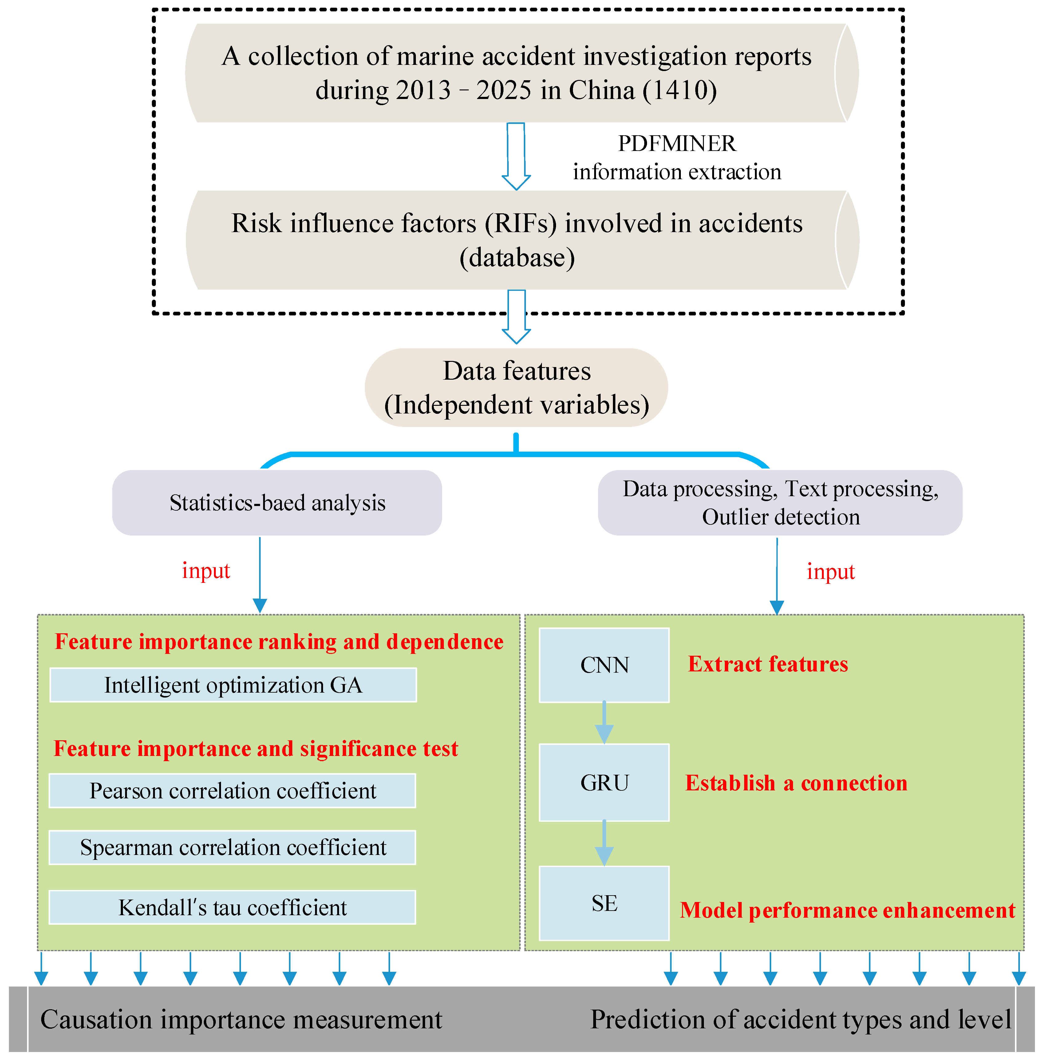
An overview of this paper is provided in Figure 2. This research contains three parts. Part I is the development of a database of risk influence factors involved in marine accidents. For this purpose, marine accident investigation reports were collected; we then extracted data features (RIFs) and labels from the database according to the requirements of running machine learning algorithms. A statistics-based analysis is conducted in Part II to investigate the data features. In Part III, we propose a comprehensive machine learning algorithm, SE-CNN-GRU, and the operation principle of this algorithm is explained in detail. The proposed algorithm was applied to investigate the potential impacts of RIFs on marine accidents and their consequences, and our interpretation of the results and a performance analysis of this algorithm are also given.

3.1. Database Establishment

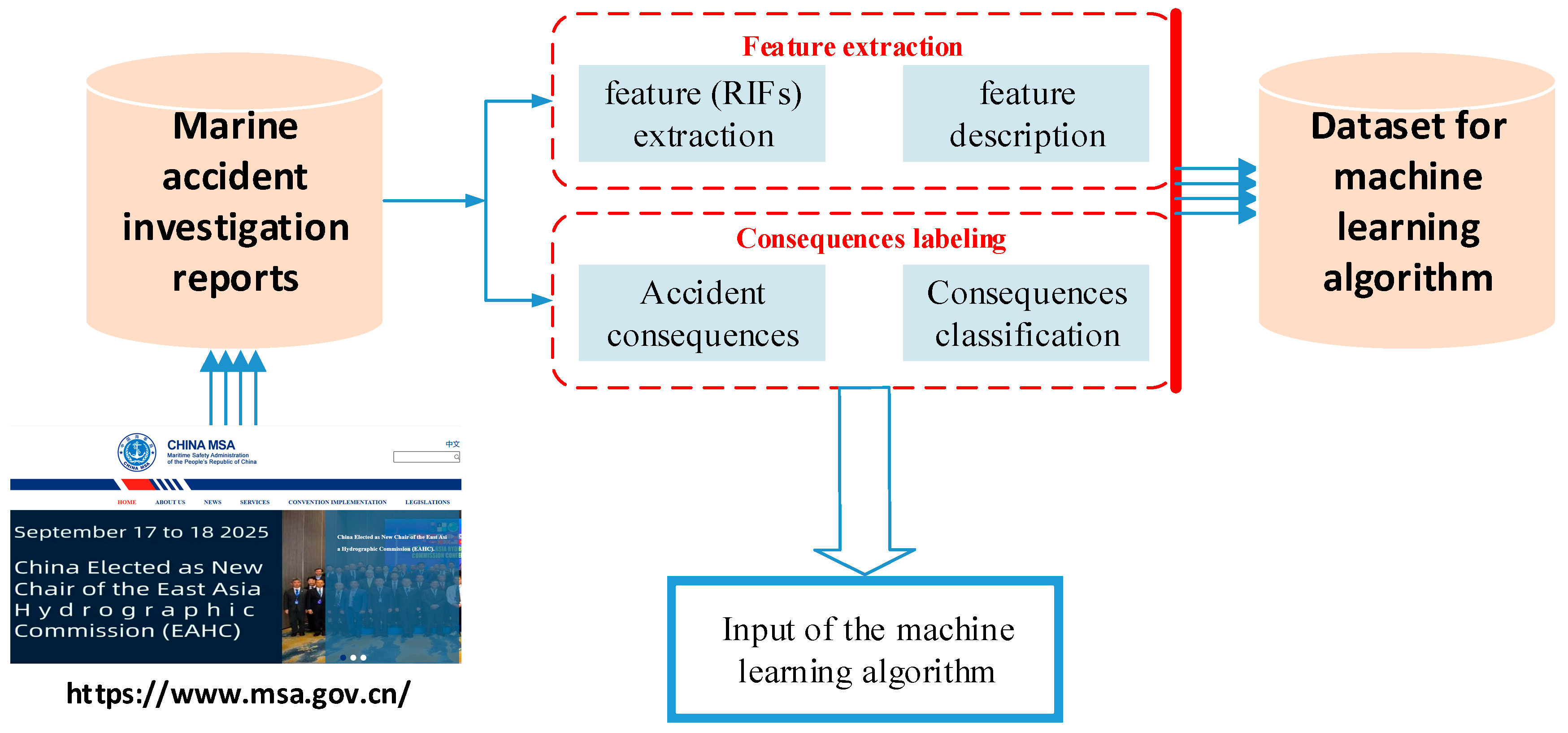
Firstly, optical character recognition (OCR) technology was used to convert the text into a PDF with machine-readable text. We then extracted the information using pdfminer and regularized expressions. The method employed in this study to make the database suitable for running a machine learning algorithm is presented in Figure 3. As shown in this figure, the first step involved obtaining marine accident investigation reports from marine accident investigation agency; then, the information associated with RIFs and accident consequences in these reports was extracted to develop a dataset for machine learning.

3.1.1. Marine Accident Investigation Report Collection

As shown in Figure 3, the marine accident investigation reports were collected from the official website of the China Maritime Safety Administration (MSA), which is the official marine accident investigation agency in China. The time span ranged from 2013 to 2024. Ultimately, we collected 1106 marine accident investigation reports. It was noted that the number of marine accidents that occurred during the 2013–2024 period was over 1106.

3.1.2. Labels for Marine Accident Consequences

In this study, the consequences of marine accidents are represented by accident type and severity. In China, the “Statistical Measure of Marine Accidents”, issued by the Ministry of Transport of the People’s Republic of China in 2021, is the official document used to define marine accident type and severity level. According to this document, marine accidents are legally classified into ten types; the ones discussed in this study are as follows: contact (T1), gale-induced accident (T2), grounding (T3), fire/explosion (T4), collision (T5), others (T6), and foundering (T7). The accident severity levels are as follows: catastrophic accident, heavy accident, and general accident. These are outlined in

Table 1. Definition of different labels for marine accident severity in this study.

Label	S1 (General Accident)	S2 (Heavy Accident)	S3 (Catastrophic)
contents	An accident that causes 1–3 deaths/missing, or 1–10 serious injuries, or direct economic losses of less than 10 million yuan	An accident that causes 3–10 deaths/missing, or 10–50 serious injuries, or direct economic losses of 10–50 million yuan	An accident that causes more than 10 deaths/missing, or more than 50 serious injuries, or direct economic losses of more than 50 million yuan

.

Therefore, each marine accident is labeled according to two different consequences, namely, accident type and accident severity, with the former comprising ten types and the latter consisting of three different levels.

3.1.3. Feature Extraction and Description

In this study, the identification of RIFs from the accident investigation reports is considered the feature extraction process. According to Ragnar Rosness [6], RIFs are factors that influence the occurrence or severity of an accident. Based on the description of accident scenarios in the accident investigation reports, the RIFs involved in the marine accidents that occurred in China during the specified period are summarized in

Table 2. Features/RIFs summary in this study.

Feature	Code	Description
Coordinate	Long. Lati.	Longitude and latitude of the marine accident
Date	Dat.	The data when the marine accident occurred
Time	Tim.	The time in a day when the marine accident occurred
Channel condition	Cha.	Mainly referring to the natural condition of the navigation channel in terms of the degree of complexity, qualified into four levels (C1, C2, C3, C4), and C4 is the most complex
Traffic density	Di (i = 1,2,3)	The number of ships appeared in the waters where the marine accidents occurred, qualified into three levels (D1, D2, D3), and D1 indicates the maximum marine traffic density
Weather	Wi (i = 1,2,…,7)	Meteorological conditions when the marine accident occurred, including sunny(W1), cloudy(W2), fog(W3), thunder shower(W4), thunderstorm(W5), moderate rain(W6), heavy rain(W7)
Sea condition	Ri (i = 1,2,3)	Mainly referring to wind, wave, and current conditions, qualified into three levels (R1, R2, R3), and R1 represents rough sea
Vessel status	Ni (i = 1,2,3,4)	The navigational status of the ships when the marine accident occurred, including underway(N1), anchoring(N2), berthing(N3), cargo handling(N4), arrival/departure(N5), operation(N6)
Vessel category	Yi (i = 1,2,…,8)	The type of the accidental ships, including multi-purpose ship (Y1), general cargo ship(Y2), engineering ship(Y3), liquid cargo ship(Y4), barge(Y5), container(Y6), passenger ship (ro/ro ship) (Y7), tug(Y8)
Cargo category	Ci (i = 1,2,…,9)	Cargoes transported by the accident ships, including passenger(C1), lashed cargo in bulk(C2), bulk solid with no liquefying(C3), bulk solid with liquefying(C4), container(C5), lashed cargo as a whole(C6), no-load(C7), liquid cargo(C8), aquatic products(C9)
Navigation area	Hi (i = 1,2,3,4)	The waters where the marine accident occurred, including coastal waters(H1), inland waters(H2), ocean(H3), cover sea waters(H4)
Ship age	Age	The years from the new building to marine accident
Tonnage	Ton.	Total tonnage recorded on the ship’s certificate
Length	LOA	The length over all (LOA) of the accidental ship

.

Prior to feature analysis and model training, the dataset underwent comprehensive pre-processing. All categorical (text-based) features, such as ‘Weather’ (W1–W7) and ‘Vessel category’ (Y1–Y8), were converted into numerical labels. Any rows containing missing values (NaN) were removed to ensure data integrity. Subsequently, all continuous numerical features (e.g., ‘Tonnage’, ‘LOA’, and ‘Ship age’) were standardized using Z-score transformation. This standardization ensured that all features contributed equally to the model’s training process by scaling them to reach a mean of zero and a standard deviation of one.

3.2. Feature Selection and Analysis

In this study, an intelligent optimization genetic algorithm (IOGA) was utilized to rank the importance of data features. Additionally, partial dependence plots (PDPs) were employed to interpret the constructed machine learning model, with the aim of understanding the relationship between the features and the target variables. As a global interpretation method, PDPs illustrate how variations in a specific feature affect a model’s prediction performance by averaging the values of all other features. This process reveals the marginal effect of an individual feature on the predicted outcome. The steps for generating a PDP are as follows:

(1)

Feature selection: Choose the feature to be interpreted.

(2)

Grid point generation: Create a series of points across the range of the selected feature’s values.

(3)

Prediction calculation: For each grid point, keep all other features constant (at their mean or actual values) and calculate the model’s predicted outcome.

(4)

Curve plotting: Plot the grid points against their corresponding predicted values to visualize the relationship between the feature and the prediction.

While PDPs are effective at showing the average impact of a feature, they overlook the interaction effects between features. Therefore, we also incorporated methods such as the Kendall correlation coefficient to calculate the influence factors among different features and conducted significance tests on the results regarding feature importance.

3.2.1. Intelligent Optimization Genetic Algorithm (IOGA)

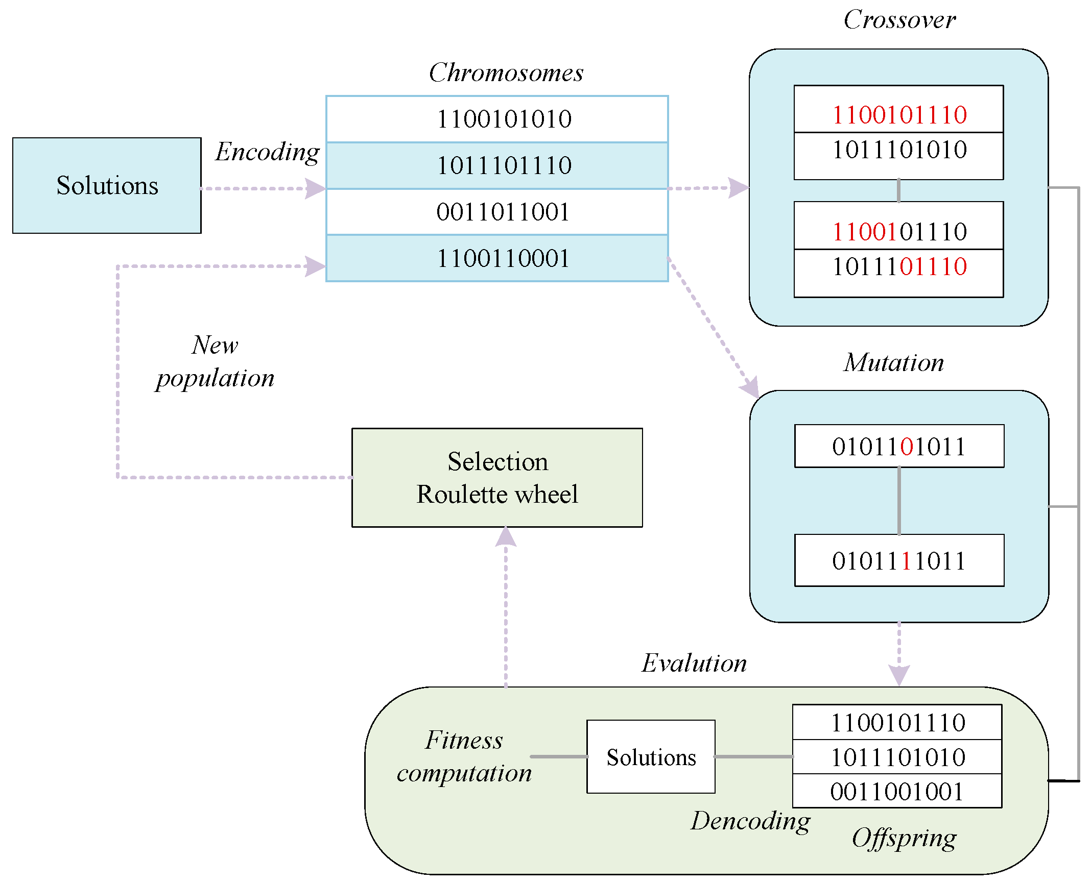
The operating mechanism of a genetic algorithm (GA) involves an iterative process that starts with a set of candidate solutions, known as a population, and the general principle is illustrated in Figure 4. Each individual solution within this population is called a chromosome. Through the application of three genetic operators (selection, crossover, and mutation), the algorithm processes the current population to generate a new population of “offspring.” The fitness of each candidate solution (chromosome) is calculated using an objective or fitness function. This function assigns a numerical score to each solution, which is then used to grade and rank the solutions within the population.

In this study, we utilized an intelligent optimization genetic algorithm (IOGA) to rank feature importance. The objective was to identify a feature subset that optimizes the algorithm’s performance metrics, such as classification accuracy or regression error. As a result, the feature selection task is transferred as a joint optimization problem. Given a dataset with features, the goal is to select a subset that yields the best performance when a model is trained on it. Each potential feature subset is represented using binary encoding. Specifically, a subset corresponds to a binary vector of length if the feature is selected and a different vector otherwise. In this work, the authors define an objective function to evaluate the impact of a feature subset on model performance, with the goal of maximizing training accuracy.

3.2.2. Spearman’s Correlation Coefficient

Spearman’s correlation coefficient is suitable for data where column features are rank variables that exhibit a linear relationship. For any two columns, e.g., column $j$ and column $k$, in a data matrix, Spearman’s correlation coefficient, denoted as $\rho$, is calculated as follows:

$$rho(a,b)=1-{\displaystyle \frac{6{\displaystyle \sum d^2}}{m\left(m^2-1\right)}}$$

(1)

where $d$ represents the difference between the ranks of the two columns, and $m$ is the length of each column. The value of the coefficient ranges from −1 to 1, where −1 indicates a perfect negative correlation and 1 signifies a perfect positive correlation between the two variables.

3.2.3. Kendall’s Tau Coefficient

Kendall’s tau coefficient, commonly denoted by $\tau$, is a rank-based correlation coefficient used to evaluate the strength and direction of the relationship between two random features based on the ranking of the data objects. It is calculated via a non-parametric hypothesis test that assesses the dependency between two random features by computing their correlation coefficient.

The coefficient $\tau$ is based on counting the number of concordant pairs in different positions within a sample. A pair of observations is concordant if their rank orderings agree. For the $j$ column and the $k$ column in a matrix, the Kendall’s tau correlation coefficient is defined as follows:

$$\tau =2{\displaystyle \frac{(n_c-n_d)}{n(n-1)}}$$

(2)

where $n_c$ is the number of concordant pairs, $n_d$ is the number of discordant pairs, and $n$ is the number of objects. The parameter $\tau$ satisfies the condition $\left[-1,1\right]$.

3.2.4. Pearson’s Correlation Coefficient

Pearson’s correlation coefficient is applied to analyze the linear correlation among different variables, particularly for continuous data samples that are normally distributed and have minor differences. Given a matrix of $m\times n$, where $m$ represents the number of feature and $n$ represents the number of samples, the correlation coefficient between two rows, row $i$ and row $j$, is defined as follows:

$$r_{ij}={\displaystyle \frac{{\displaystyle {\sum }_{k=1}^n\left(x_{ik}-{\overline{x}}_i\right)\left(x_{jk}-{\overline{x}}_j\right)}}{\sqrt{{\displaystyle {\sum }_{k=1}^n{\left(x_{ik}-{\overline{x}}_i\right)}^2{\displaystyle {\sum }_{k=1}^n{\left(x_{jk}-{\overline{x}}_j\right)}^2}}}}}$$

(3)

where $n$ is the length of each row. The value of the coefficient ranges between −1 and 1. A value of −1 indicates a complete negative correlation, while a value of 1 denotes a complete positive correlation. If the coefficient is 0, it signifies that there is no correlation between the two rows.

3.3. Principle of the Proposed Methodology

SE-CNN-GRU is a composite architectural model designed to overcome the limitations of individual models by integrating their respective strengths. It organically combines feature extraction, adaptive feature significance weighting, and sequential dependency modeling to form a powerful end-to-end learning framework. The synergistic way in which this architecture operates is illustrated in Figure 5, which graphically depicts the complete data-processing procedure from input to output. This model involves the analysis of dataset features using IOGA, the vectorization of raw features within the CNN, and data preprocessing and reshaping, thereby converting multi-dimensional feature vectors into a tensor format suitable for one-dimensional convolutional neural network processing. The general functional principles of CNNs, GRU, and SE are outlined in this section.

In this study, the 14 RIFs (features) described in Table 2 are not treated as a simple flat vector. Instead, to leverage the strengths of the hybrid architecture, the input data for each accident are given as a (14, 1) sequence. As shown in

Table 3. Main architecture and partial parameter of the SE-CNN-GRU algorithm.

Layer Type	Hyperparameters	Output Shape	Purpose
Input Layer	Number of Features: 14	(Batch Size, 14, 1)	Receives raw maritime accident data.
Zerocenter	Number of Features: 14	(Batch Size, 14, 1)	Normalization processing of data
Convolutional (Conv.)	Filters: 32, Kernel Size: 3, Activation: ReLU	(Batch Size, 12, 32)	Extracts associative patterns between local features.
Batch Norm	Batch: 12	(Batch Size, 12, 32)	Controls overfitting, aids convergence
Pooling	Pool Size: 2	(Batch Size, 6, 32)	Performs down-sampling to create robust features invariant to small shifts.
SE Module	Reduction Ratio: 4	(Batch Size, 6, 32)	Adaptively recalibrates channel-wise feature responses.
GRU Layer	Units: 64	(Batch Size, 64)	Model dependencies within the feature sequence.
Fully Connected (Dense)	Units: 32, Activation: ReLU	(Batch Size, 32)	Combines high-level features for classification.
Dropout Layer	Dropout Rate: 0.5	(Batch Size, 32)	Regularization to prevent overfitting.
Output Layer (Dense)	Units: N_Classes, Activation: Softmax	(Batch Size, N_Classes)	Produces the final probability distribution over accident level and type.

, this sequence is first fed into the model.

The data-processing steps are as follows:

(1)

The “1D-CNN layer” (with a kernel size of 3) slides across this 14-feature sequence. Its primary purpose is not to model time-series data but to automatically extract complex, localized associative patterns between adjacent features (e.g., how the combination of ‘Longitude’, ‘Latitude’, and ‘Channel condition’ might form a specific risk pattern).

(2)

The feature maps generated by the CNN (32 channels) are then passed to the ‘SE Module’. This module performs feature re-calibration, adaptively learning to ‘excite’ (amplify) the importance of the most predictive patterns (channels) and ‘squeeze’ (suppress) the less useful ones for that specific accident.

(3)

This re-weighted sequence of features is then fed into the **GRU layer**. The GRU models the higher-order sequential dependencies between these extracted, weighted features.

(4)

Finally, the output of the GRU is passed through a dense layer for the final classification (accident severity or type).

This architecture is intentionally designed to capture the deep, non-linear interdependencies between RIFs, which a standard flat model (like RF or SVM) might miss.

3.3.1. The Operating Principle of a CNN

The CNN feature extraction module consists of a series of one-dimensional convolutional layers (Conv1D) and pooling layers. The convolutional layers extract associative patterns between local features using sliding filters, while the pooling layers perform down-sampling on the feature maps to enhance model generalization and reduce computational complexity.

A convolutional neural network (CNN) is a specialized neural network model designed for processing two-dimensional data, such as images. The process begins with using a training dataset composed of samples with labeled features and corresponding class labels to build the CNN model. The core of a CNN is the convolutional layer, which extracts features through convolution operations. This layer utilizes a set of learnable filters, also known as kernels, that slide across each sample in the dataset to compute convolution results at each position, generating a set of feature maps where each map corresponds to a specific filter:

$$y_{t,j}={\displaystyle \sum _{i=1}^k{x}_{t+i-1}\cdot w_{i,j}}+b_j$$

(4)

where $y_{t,j}$ represents feature $j$ of the output feature map at time step $t$; $x_{t+i-1}$ is the area corresponding to the convolutional kernel coverage in the input data quantity; $k$ is the size of the convolution kernel; and $w_{i,j}$ denotes the weights of the convolution kernel; and $b_j$ is the bias item.

After the convolutional layer, a non-linear activation function, such as ReLU, is typically applied to introduce non-linearity. A pooling layer is then used to reduce the dimensionality of the feature maps, which decreases the computational load while retaining essential features. After the data pass through multiple convolutional and pooling layers, a set of high-level feature representations is obtained. These features are subsequently mapped to class labels by a fully connected layer:

$$y=W\cdot x+b$$

(5)

where $W$ is the weight matrix; $x$ is the input vector; $b$ is the bias term; and $y$ is the output.

The network’s prediction error is measured by a loss function, and an optimization algorithm, such as a stochastic gradient descent, is employed to adjust the network’s parameters to minimize this loss. The model’s classification performance is progressively improved by repeatedly performing forward and backward propagation to adjust network parameters. Finally, for a new dataset that requires classification, the data are fed into the trained CNN via a forward propagation step to produce an output. The data are then assigned to the class corresponding to the highest output value, which constitutes the final classification result.

3.3.2. Principle of SE Module

The SE attention module takes the features output by the CNN module as its input. Through a ‘Squeeze’ operation (global average pooling) and an ‘Excitation’ operation, it generates an importance weight for each feature channel. These weights are then applied to the original features via a ‘Scale’ operation, achieving the adaptive re-calibration of the features.

Squeeze-and-excitation (SE) is a dual-channel dot-product attention strategy designed to improve the representational power of a network. Its core principle consists of explicitly modeling the interdependencies between channels. By learning to selectively emphasize informative features and suppress less useful ones, the SE module allows the model to re-calibrate its feature responses on a channel-by-channel basis.

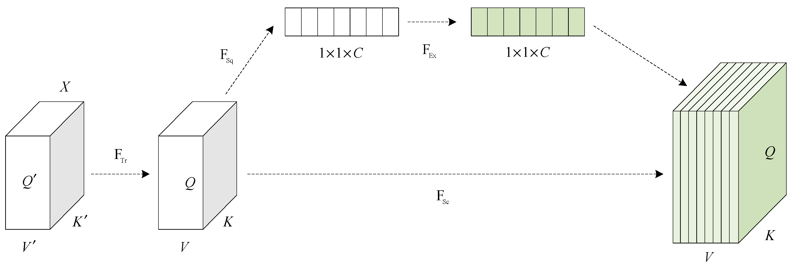
The workflow of the SE module is shown in Figure 6; it comprises four parts: transformation, squeezing, excitation, and scaling.

Assuming that the input feature sequence $X\left(1\times 1\times C\right)$ undergoes linear transformation, the query and key values of the input features in the feature sequence are Q, K, and V, respectively:

$$\begin{array}{ccc}Q=X{W}^Q& K=X{W}^K& V=W^Q\end{array}$$

(6)

The attention scores under dual channels are $A_1$ and $A_2$, respectively:

$$A_1=\mathrm{softmax}\left({\displaystyle \frac{Q\cdot K^T}{\sqrt{d_k}}}\right)V$$

(7)

$$A_2=\mathrm{softmax}\left({\displaystyle \frac{Q^{\prime }\cdot {K^{\prime }}^T}{\sqrt{d_{k^{\prime }}}}}\right)V^{\prime }$$

(8)

The final score A of a channel is the weighted sum of two channels:

$$A=\alpha A_1+\beta A_2$$

(9)

where $\alpha$ and $\beta$ are weight parameters obtained through learning, and the final output result of the channel is as follows:

$$\mathrm{Output}=A\cdot V$$

(10)

3.3.3. Principle of GRU

The GRU sequential modeling module receives the weighted feature sequence from the SE module. The GRU layer processes these feature vectors step by step, capturing long-range dependencies within the sequence through its internal gating mechanisms (update and reset gates).

Finally, the classification head takes the final hidden state vector output by the GRU layer after processing the entire sequence as its input. This module typically consists of one or more fully connected (dense) layers, culminating in a SoftMax activation function layer that outputs a probability distribution over the different classes. The class with the highest probability is the model’s final prediction.

The gated recurrent unit (GRU) is a streamlined recurrent neural network architecture designed to model sequential data efficiently. Compared to LSTM, the GRU reduces complexity by consolidating gating mechanisms into two adaptive gates, i.e., the update and reset gates, while retaining robust long-term dependency modeling.

The update gate regulates the retention of historical information:

$$z_t=\sigma \left(W_Z\cdot \left[h_{t-1},x_t\right]\right)$$

(11)

where $z_t\in \left[0,1\right]$ determines the balance between the prior hidden state $h_{t-1}$ and the new inputs $x_t$, with $\sigma$ being the sigmoid function.

The reset gate controls the influence of past states on candidate updates:

$$r_t=\sigma \left(W_r\cdot \left[h_{t-1},x_t\right]\right)$$

(12)

A candidate state ${\tilde{h}}_t$ is then computed as follows:

$${\tilde{h}}_t=\tanh \left(W\cdot \left[r_t*h_{t-1},x_t\right]\right)$$

(13)

where * denotes element-wise multiplication.

The final hidden state $h_t$ merges historical and candidate states via the update gate:

$$h_t=\left(1-z_t\right)*h_{t-1}+z_t*{\tilde{h}}_t$$

(14)

When $z_t\approx 1$, the GRU preserves prior information; when $z_t\approx 0$, it prioritizes current inputs. This dual-gated design enhances computational efficiency while mitigating gradient issues in sequential modeling.

To provide a clear and reproducible technical specification, in Table 3, we summarize the main hierarchical structure and key parameter configurations of the entire SE-CNN-GRU model. This table is key to understanding the model’s data flow and transformations, serving as a blueprint for anyone wishing to replicate the model’s work.

The proposed SE-CNN-GRU network, along with the baseline GRU, was trained using the Adam optimizer, which is well-suited to deep learning tasks. Based on iterative tuning, the key hyperparameters were set as follows: the ‘initial learning rate’ was set to ‘0.001’, the ‘batch size’ was set to ‘64’, and the models were trained for a maximum of ‘3500 epochs’. A dropout layer with a rate of 0.5 (as listed in Table 3) was included to mitigate overfitting. In the training for baseline models (RF, XGBoost, and SVM), their respective standard hyperparameter-tuning processes were used. Based on the architecture defined in Table 3, the proposed SE-CNN-GRU network contains approximately “21,615” trainable parameters. Given the dataset size of 1106 samples, rigorous overfitting control is essential. This was managed through three primary mechanisms:

(1)

Architectural regularization, including “Batch Normalization” and a “Dropout layer (0.5)”;

(2)

The use of the “Adam optimizer” with a tuned “learning rate (0.001)” and “batch size (64)”, trained for 3500 epochs;

(3)

Most critically, the adoption of a “10-fold Cross-Validation” protocol (would be described in Section 4.2), which provides a robust and unbiased estimate of the model’s generalization performance on the available data.

4. Results Analysis

4.1. Database Description

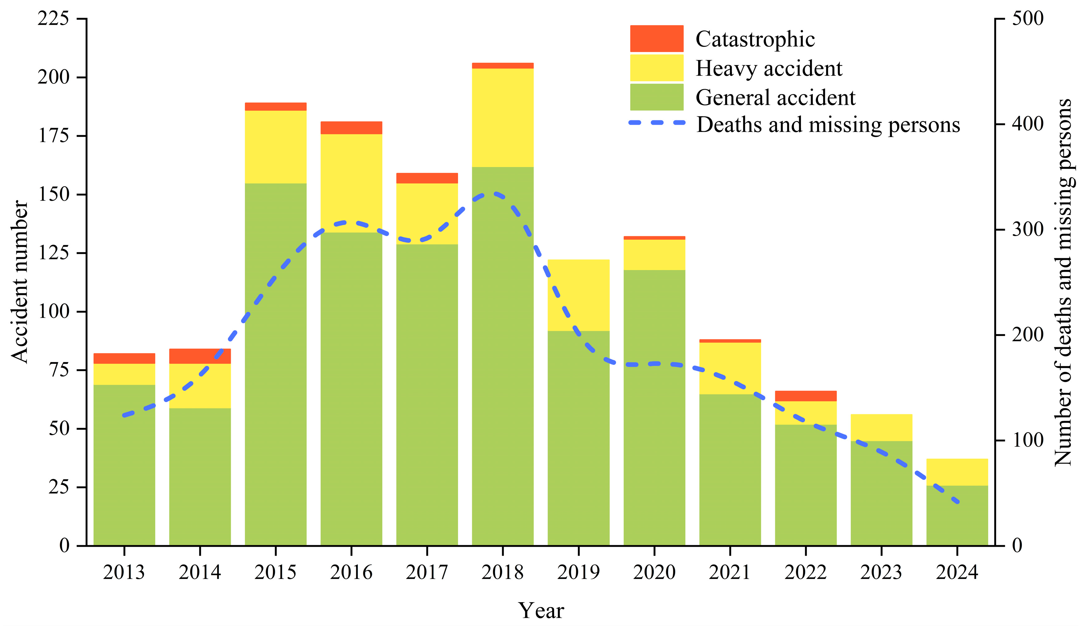
In this study, we collected 1106 marine accident investigation reports issued by China’s MSA during the 2013–2024 period, which predominantly contained seven types of accidents. The number of accidents for each accident type is presented in Figure 7, as is the number of deaths/missing people resulting from each type of accident.

According to Figure 7, the losses and number of accidents within Chinese waters has decreased since 2018, despite the increasing trend from 2013 to 2018, especially for catastrophic accidents. The reason for this is mainly the significant efforts carried out by the Chinese MSA to mitigate such disasters. In addition, the decrease in marine accidents is also a result of the optimization of the total ship fleet in China; according to the statistics issued by the Ministry of Transport of China, the average gross tonnage has greatly increased in recent years (detailed annual information can be found in the “Statistical Bulletin on the Development of the Transportation Industry in China”). However, both the number of marine accidents and accidental losses in China are higher than in many other countries, such as England and the United States. This may be explained by the total size of the ship fleet and the complex navigational waters in China. To further investigate the distribution of the marine accidents that occur in Chinese waters, all the marine accidents contained in the database are geographically presented in a visual manner, as illustrated in Figure 8. Figure 8a illustrates the distribution of these marine accidents that occurred during the day, while the distribution of marine accidents that occurred at night is presented in Figure 8b. When comparing Figure 8a,b, a number of patterns can be observed; these are summarized as follows.

(1)

Marine accidents are geographically concentrated both during the day and at night; specifically, almost all marine accidents in China occur in the waters of Bohai Bay, the Yangtze estuary, the Zhoushan Islands, the Taiwan Strait, the Pearl River estuary, the Qiongzhou Strait, and the Yangtze River, all of which can be collectively and concisely dubbed “six zones and one river”.

(2)

More marine accidents occur at night than during the day, especially catastrophic and severe accidents, which are marked by red and yellow in Figure 8. In addition, catastrophic and severe accidents mainly take the form of ship collision and foundering, which can easily lead to a high number of deaths/missing persons.

(3)

Safety management in Yangtze estuary and the Pearl River estuary should be given considerably more attention due to the heavy losses of life that occur there, especially at night. The reason for this may partly lie in the heavy marine traffic that is present in these two areas.

In this study, the calendar heat map for the collected marine accidents is prepared and the results are presented in Figure 9. Generally, there is no obvious pattern can be observed from the calendar heat map. However, some differences can be summarized according to the calendar distribution of these marine accidents. For instance, the accident number in February is less that of other months, and the accident number in August and October is slightly more than other months, which may be attribute to the fishery activities within China’s coastal waters.

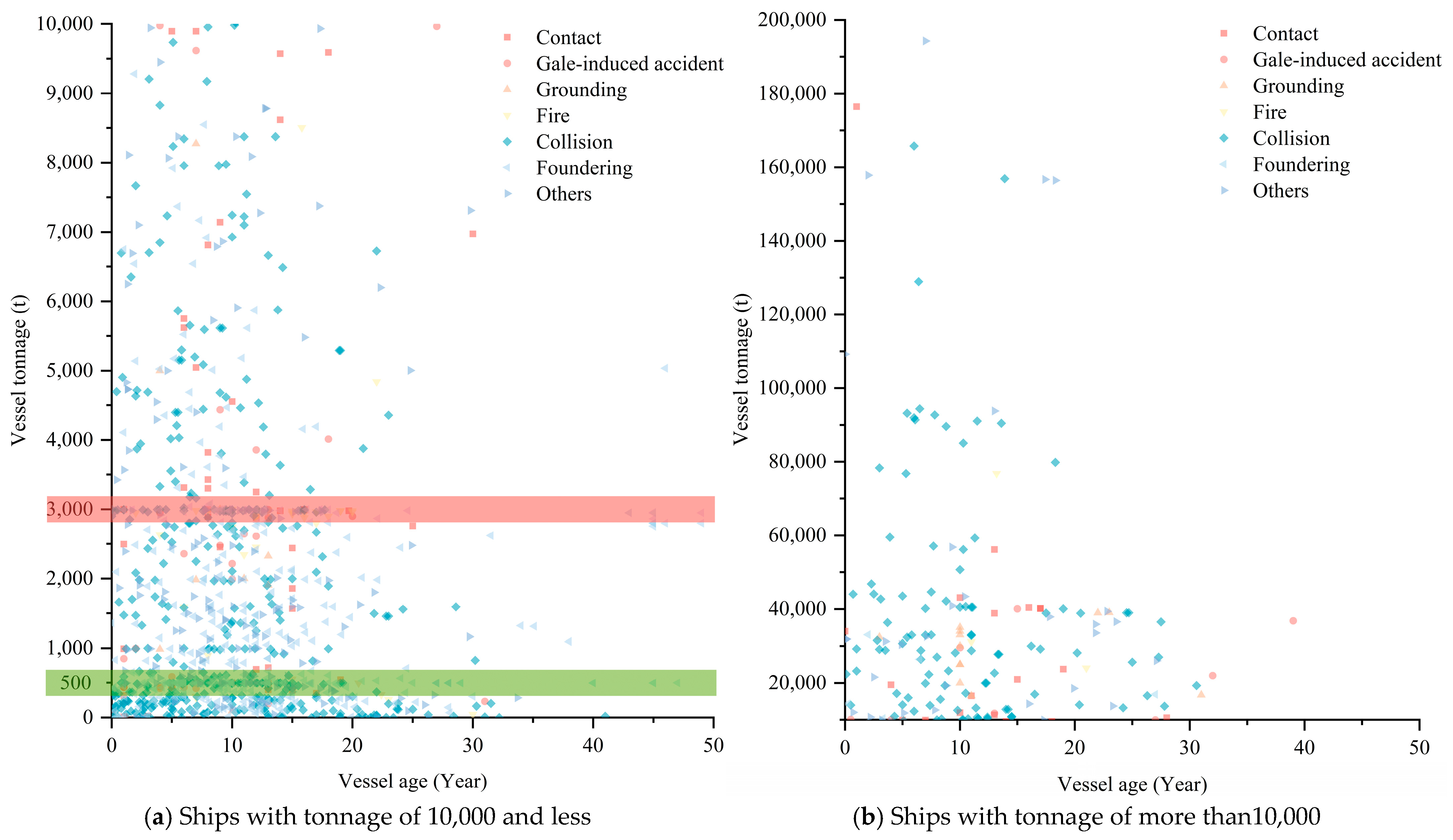
According to the database, there were a total of 1200 ships involved in these marine accidents. The tonnage and age of each ship in relation to the different types of accidents are illustrated in Figure 10, which can be interpreted as follows.

(1)

The tonnage of ships involved in overall accidents is usually less than 10,000 tons, while the ships involved in collision accidents generally had a tonnage above this weight; collisions mainly occurred between large merchant vessels and fishing ships.

(2)

Differences in age for various types of accidents can be observed to some extent. For example, the median and upper limits of ship age for ‘foundering’ and fire/explosion accidents are relatively higher, indicating that older vessels may be more prone to such severe incidents.

(3)

When focusing on the tonnage distribution of ships involved in accidents, it is interesting to observe the ‘two lines’ in Figure 10b: one represents 500 total tons (represented by green bar), and the other represents 3000 total tons (represented by red bar). These development of these two lines is mainly due to maritime regulations in China: the total tonnages of 500 and 3000 are set as the threshold values for ships, with different maritime regulations being applicable.

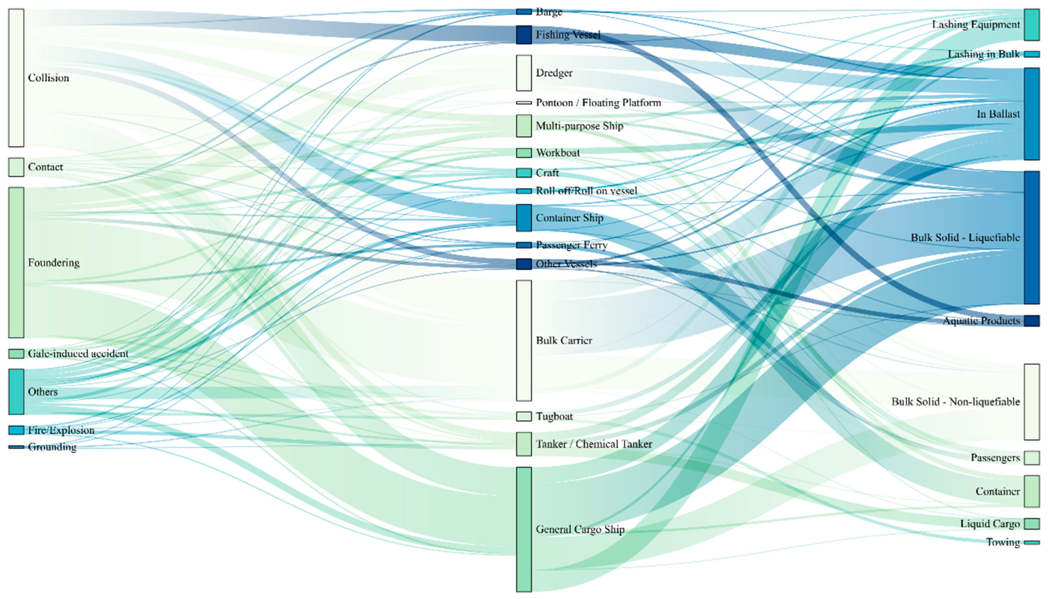
The number of and relationships between different types of marine accidents, ships, and cargo were statistically analyzed utilizing the database developed in this study, and the results are presented in the form of a Sankey diagram, which is illustrated in Figure 11. It should be noted that the heights of rectangular boxes indicate the percentages. For instance, in terms of the types of marine accidents, the rectangular box that denotes foundering is the highest, and the box that denotes collisions is the second highest, indicating that foundering and collision accidents were the most frequent marine accidents in Chinese waters during the 2013–2024 period. Statistically, collision and foundering accidents account for 30% and 45% of total marine accidents, respectively. Similarly, when it comes to ship types, bulk cargo ships and general cargo ships have the highest number of accidents, with a significant proportion of foundering accidents, while the ships carrying cargo of the “bulk solid—liquefiable” class are more prone to marine accidents. In addition, as shown by the relationships presented in Figure 11, collisions are the main cause of accidents involving fishing vessels, accounting for over 90% of accidents. The proportion of foundering accidents in barge-related accidents is relatively high, accounting for about 35% of accidents involving this type of ship. The proportion of fire/explosion accidents involving oil tankers/chemical tankers is relatively high, accounting for about 15% of accidents involving this type of vessel. It should be noted that there is a very high correlation between “bulk solid—liquefiable” cargo ships and foundering accidents, as shown in Figure 11.

To explore the relationship between accident time and the statuses of the ships, in this study, these two data features (time and navigational status) are exclusively abstracted into a box-and-violin plot, the results of which are presented in Figure 12.

In accordance with Figure 12, it can be observed that the ships with “underway” status have the highest number of accidents in all time periods. In terms of the ships with “anchoring” status, these ships are more prone to marine accidents during the early morning hours, such as 4 o’clock in the morning. When it comes to the ships with “arrival/departure” status, marine accidents generally occur slightly after noon, and a similar phenomenon can also be observed in the case of vessels with “berthing” status. In addition, marine accidents associated with cargo handling are frequently observed in the morning, such as around 10 o’clock, which may be a result of the port being in operation at this time. When it comes to the various operations on board the ships, it can be observed that the accidents are prone to occur around noon; from a practical perspective, this may be because operators/crew are easily tired at noon, and shifts are frequently paused due to lunch, possibly resulting in a lack of vigilance among personnel.

4.2. Experimental Results Analysis

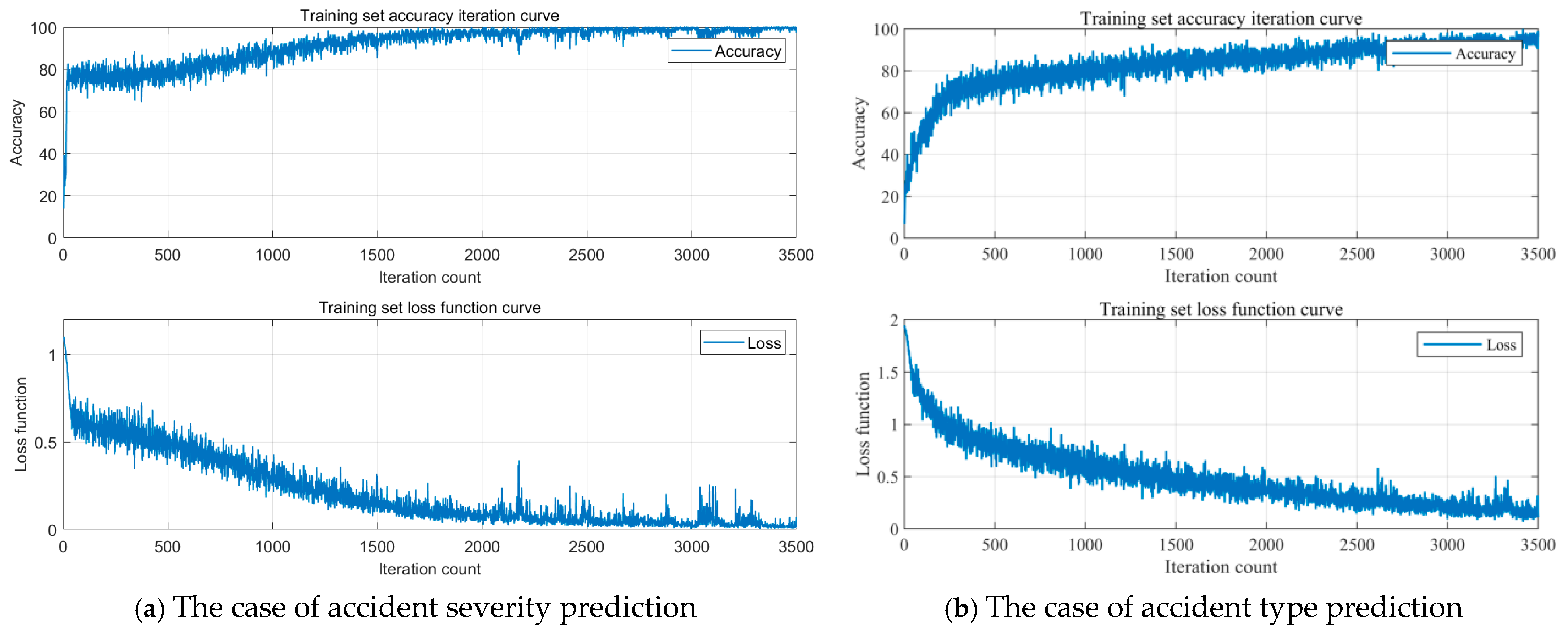
Before conducting our experiments on the computing platform, we allocated 80% of the dataset to be training data, while the remaining 20% of the dataset was used as the test data. The software environment for running the algorithms developed in this study is summarized in

Table 4. Software environment setup in this study.

Item	Specifications
CPU	12th Gen Intel(R) Core(TM) i5-12490F 3.00 GHz (Intel Corporation, Santa Clara, CA, USA)
GPU	NVIDIA GeForce GTX 1660 (6 GB) (Nvidia Corporation, Santa Clara, CA, USA)
RAM	32 GB
Language	Python 3.9.21, Matlab R2024a
Operating system	Windows 10 × 64 bit
ML Framework	Tensorflow 2.18.0, pytorch-lightning 2.4.0, keras 3.6.0

, and the pseudo-code for the running of this proposed SE-CNN-GRU algorithm can be found in Appendix A. Regarding the convergence of the proposed SE-CNN-GRU algorithm, the loss and accuracy of this algorithm can be found in Figure 13. Figure 13a illustrates the convergence of SE-CNN-GRU algorithm for marine accident level prediction, while the results for accident type prediction are presented in Figure 13b. Comparing the results presented in Figure 13a,b reveals that the accuracy and loss of the proposed SE-CNN-GRU algorithm for accident level prediction are better than those for accident type prediction. Therefore, the proposed comprehensive machine learning algorithm is more suited to conducting marine accident level prediction.

Feature Analysis

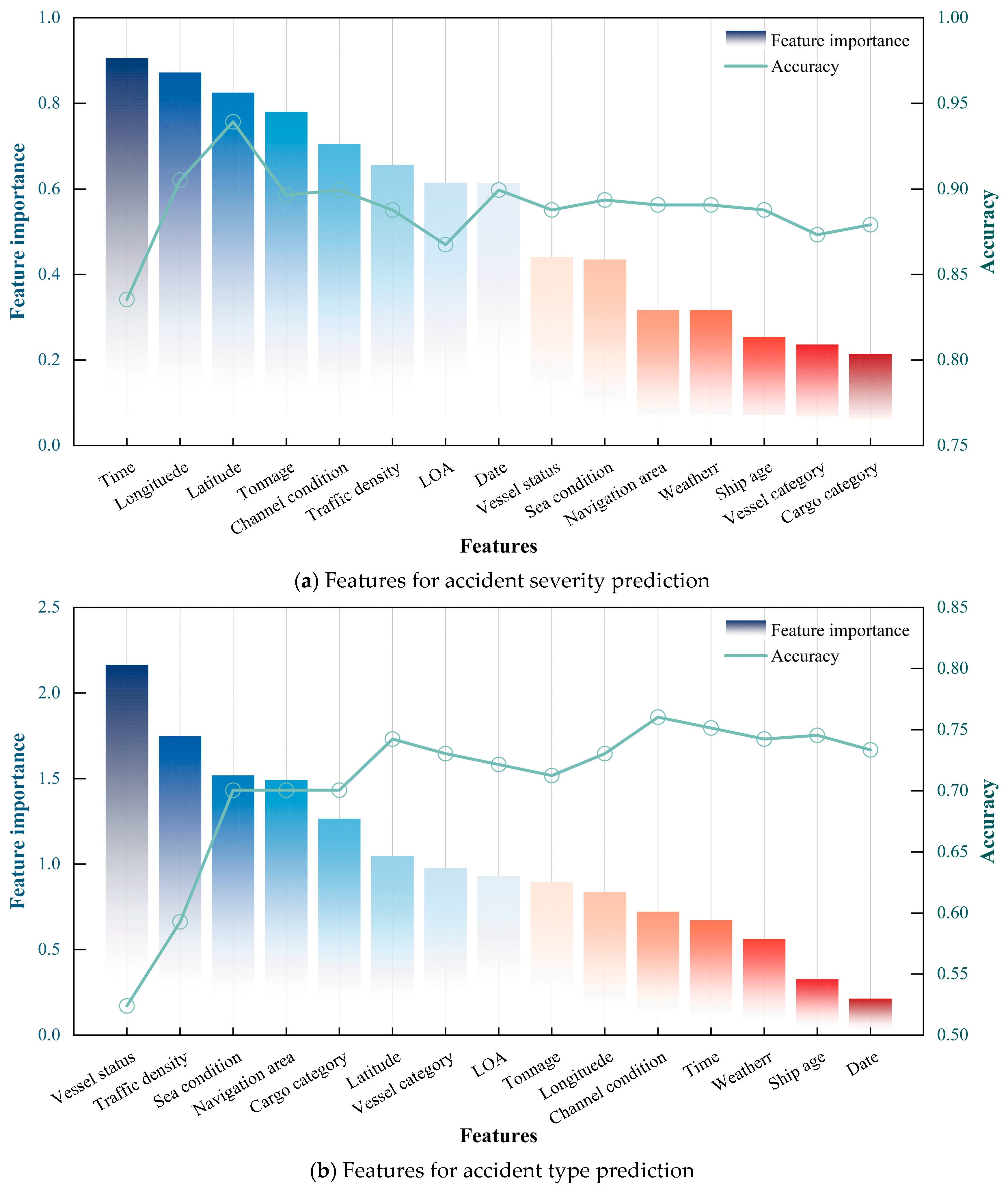
The feature analysis in this study was first conducted in terms of feature importance and accuracy by means of IOGA, the results of which are presented in Figure 14. The column bars in Figure 14 indicate the importance values for each feature, and the scattered dots in Figure 14 represent the accumulative prediction accuracy; obviously, the prediction accuracy would not continuously increase with the addition of data features. According to Figure 14a, when aimed at marine accident severity prediction, the features of “time”, longitude, and latitude had high importance, while the cargo category, vessel category, and ship age had low importance. This was especially the case for the time feature, whose importance was verified by the results presented in Qiao et al. [5]. Specifically, marine accidents are more likely to occur at night, when the precaution levels of the crew on watch are lower than at other times. In terms of longitude, in Chinese waters, in some ways this feature represents the distance from the coastline, which means that the farther away from the coastline, the more likely serious marine accidents are to occur. Moreover, the prediction accuracy would not increase with the addition of features; for instance, the consideration of features whose importance is lower than that of date would not improve the prediction accuracy. Therefore, in this study, the features with larger importance values than that of date are considered the most important features. The results of the feature analysis in terms of accident type prediction are presented in Figure 14b. According to Figure 14b, the vessel status feature is obviously more important than the others; however, its prediction accuracy is extreme low. It should be noted that the prediction accuracy would continuously increase with the addition of further data features. Sea conditions and traffic density are also important for accident type prediction, with importance values that are slightly lower that of vessel status, and the features of ship age and date are the least important in terms of accident type prediction. Considering the addition of data features would have negative impacts on the running of the algorithm, such as consuming more time and occupying more calculation resources, in this study, the data features with larger importance values than that of time were considered important features. By comparing Figure 14a,b, obvious differences can be found regarding accident severity prediction and accident type prediction. For instance, location information (longitude and latitude) is regarded as an important feature for accident severity prediction, but it is less important for accident type prediction. In addition, the prediction accuracy for accident type is always lower than that of accident severity even though all the data features are considered.

Another aspect of feature analysis in this study is the correlation represented by Spearman’s correlation, Kendall’s tau, and Pearson’s correlation coefficients discussed in Section 3.2. The results are visually presented in Figure 15 in form of heat-map. The different colors within Figure 15 represent the relationships between the feature subcategories. Specifically, the size of the hexagon and the depth of the color blocks indicate the strength of the correlation between two features. The larger the shape and the darker the color, the stronger the correlation between the two features. In addition, the asterisks indicate the degree of significance of the results. “***” indicates an extremely significant correlation; “**” indicates a highly significant correlation; and ‘*’ indicates a significant correlation between the results. Significant correlations of the results represent the reliability of the feature correlation results. When the significant correlation is low, it indicates that the obtained feature correlation may only be random, which has no statistical significance.

Focusing on the results with significant correlation, it can be seen from Figure 15 that in marine accidents, the tonnage and length of the ships involved in the accidents, as well as the channel conditions and traffic density, all have strong correlations. This indicates that the reliability of the data is strong and in line with general logic. The strong correlation between latitude and longitude, especially longitude and navigation area, indicates that the areas where ship accidents occur are relatively concentrated, and the distribution pattern in longitude is strong. There is also a significant correlation between ship tonnage, cargo category, and ship category, indicating that the category of ships and cargo categories involved in accidents are relatively concentrated. At the same time, there is a level of correlation between the cargo category, navigation area, date, ship status, traffic density, longitude, etc.

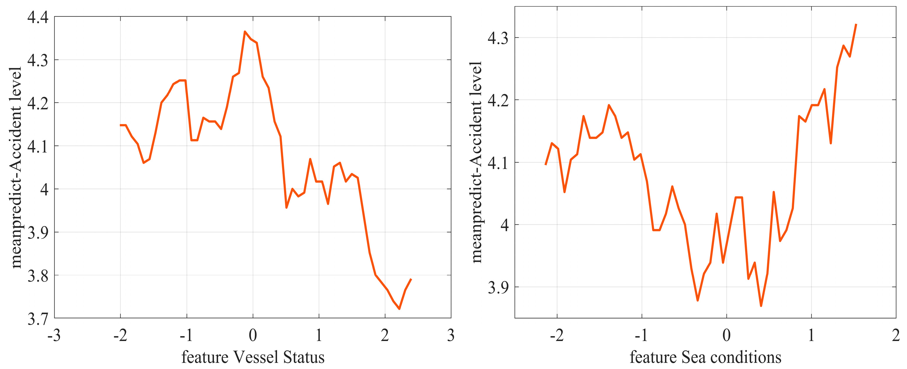
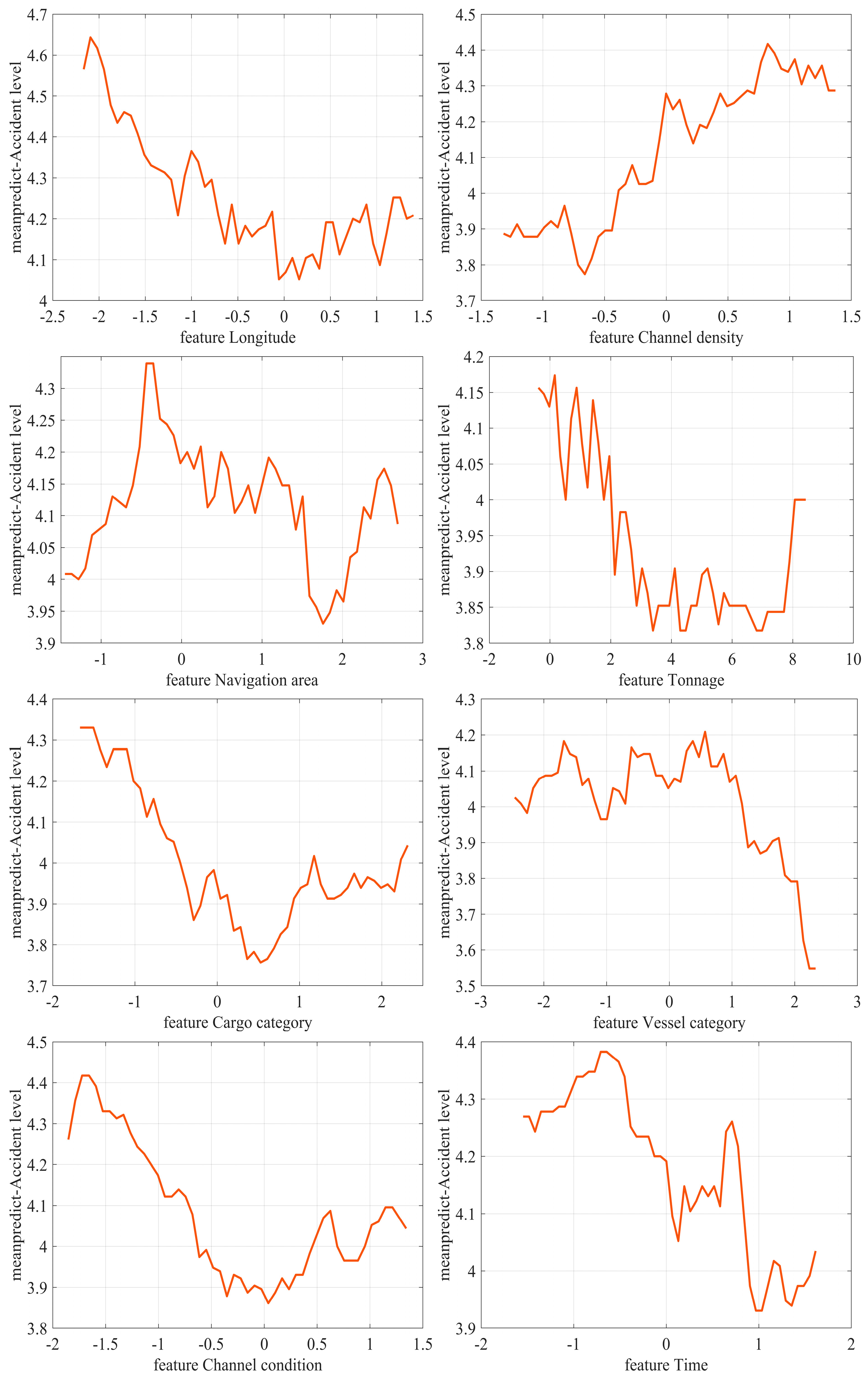
According to Friedman [54], the figures of PDP are used to visualize the marginal effect of a specific data feature on the prediction performance of an algorithm with the consideration of the average effect of other data features. In this study, the PDP values of important features for accident severity prediction and accident type prediction are, respectively, calculated, and the results are presented in Figure 16 and Figure 17, respectively. In these figures, the x-axis represents the standardized values of features, and y-axis corresponds to the partial dependence values. It can be noted that a higher partial dependence value implies that the feature tends to drive the algorithm to make a prediction of the occurrence of marine accidents.

On the basis of PDPs values of these important features for accident severity prediction and accident type prediction, the roles of important features for the accident consequences can be further presented and discussed. For instance, the time feature is considered the most important feature in terms of accident severity prediction. According to the feature of time in Figure 16, the variation in partial dependence values is represented by “V” with an increase in time from 0 AM to 12 PM, which indicates that the likelihood of a marine accident would decrease first, and the likelihood would raise later. During the middle of the day, the likelihood of marine accidents occurring is the lowest. However, it was observed that the accident risk in the early morning was the highest; therefore, port management officers or officers in vessel traffic service centers should pay much attention to shipping activities during this time. Ff necessary, additional human resources may be needed. Similar patterns can also be observed for the longitude feature. Another noteworthy feature is the LOA of the accidental vessels; the results of the PDP calculation are presented in Figure 16g. A relatively clear decrease in partial dependence values can be observed with the increase in the standardized vessel LOA, which indicates that the vessels with small LOA are more prone to marine accidents in China’ waters. When it comes to the channel density feature (Figure 16f), it was found that waters with high channel density are characterized by high accident risk; therefore, it is advised to conduct strict vessel traffic management within waters with high channel density, such as the Yangtze estuary.

It should be kept in mind that these results illustrated in Figure 16 and Figure 17 and associated with PDP calculations can be used to provide meaningful insights into how important features (RIFs) influence marine accident consequences using the comprehensive machine learning algorithm proposed in this study (SE-CNN-GRU). However, in practice, the improvement of marine safety management should also take many other factors into account, which are discussed in the following section.

4.3. Prediction Performance and Comparative Analysis

To rigorously evaluate the generalization performance of the proposed SE-CNN-GRU model and objectively position it against established methods, we implemented a comprehensive comparative analysis. All models were assessed using a 10-fold cross-validation (CV) protocol to mitigate potential overfitting and to provide a statistically robust measure of performance on the 1106-sample dataset.

In addition to the proposed SE-CNN-GRU, four baseline models were included for comparison: random forest (RF), XGBoost, support vector machine (SVM), and a standard GRU (without the CNN and SE components). The mean accuracy and standard deviation for both prediction tasks across all 10 folds are presented in

Table 5. Comparative Model Performance using 10-fold Cross-Validation (Accident Type).

Model	Accuracy	Precision	Recall	F1 Score	Specificity	10-Fold CV Accuracy (Mean)	10-Fold CV Accuracy (Std. Dev.)
SVM	0.77391	0.56856	0.49045	0.51017	0.92883	0.72632	0.037266
XGBoost	0.66087	0.44657	0.34738	0.35501	0.91290	0.66626	0.050323
GRU	0.76957	0.51688	0.43569	0.45485	0.94808	0.76470	0.037300
RF	0.73043	0.35784	0.39292	0.37375	0.91818	0.70707	0.064002
SE-CNN-GRU	0.80217	0.55582	0.48620	0.48333	0.89089	0.82595	0.041821

and

Table 6. Comparative Model Performance using 10-fold Cross-Validation (Accident Severity).

Model	Accuracy	Precision	Recall	F1 Score	Specificity	10-Fold CV Accuracy (Mean)	10-Fold CV Accuracy (Std. Dev.)
SVM	0.90870	0.94618	0.79229	0.85314	0.88121	0.93466	0.034726
XGBoost	0.91739	0.95057	0.80647	0.86507	0.89333	0.94252	0.021772
GRU	0.89565	0.92469	0.78139	0.83886	0.87150	0.92943	0.018675
RF	0.92609	0.95489	0.82066	0.87653	0.90545	0.95119	0.016630
SE-CNN-GRU	0.93435	0.94869	0.83076	0.88064	0.92210	0.93858	0.032528

.

The comparative results for the 3-class accident severity prediction task are presented in Table 6. The analysis indicates that all models achieved a high level of performance. The proposed SE-CNN-GRU model (0.9386 ± 0.0325) demonstrates excellent and robust predictive power. Its performance is highly competitive with the top-performing traditional models, Random Forest (0.9512 ± 0.0166) and XGBoost (0.9425 ± 0.0218). The marginal difference in accuracy (approx. 1.2% against RF) is likely not practically significant, confirming that for this simpler 3-class task, a well-tuned ensemble model like RF is an efficient and appropriate choice.

The true utility and usefulness of the SE-CNN-GRU architecture becomes evident in the more complex 7-class accident type prediction task, as detailed in Table 5. In this more challenging scenario, the SE-CNN-GRU model (0.8260 ± 0.0418) achieves markedly superior performance. It outperforms the next-best model (baseline GRU, 0.7647) by over 6% and, critically, outperforms the best traditional models (SVM, 0.7263; RF, 0.7071) by “10–12%”. This performance gap is practically significant and strongly indicates that the hybrid architecture, which combines CNN, SE, and GRU, is uniquely capable of capturing the subtle, non-linear dependencies between the 14 RIFs required to classify complex accident types. While simpler models fail to model this interplay, the SE-CNN-GRU architecture excels. This directly answers why the hybrid model is useful, as its value lies in solving the more complex, multi-class problem that simpler models cannot. By comparing the content in Table 5 and Table 6, it can be observed that there is nearly no competitiveness of the proposed SE-CNN-GRU algorithm over the traditional single machine learning algorithm, such as RF in terms of accident severity prediction based on the practical significance. However, when it comes to accident type prediction, the performance of the proposed SE-CNN-GRU algorithm in this study obviously has an advantage over the traditional machine learning algorithms, such as RF and XGBoost, which indicates the application potentials in the maritime safety management.

Notably, the ensemble models (RF and XGBoost) that performed marginally better on the simpler severity task were not effective here (0.7071 and 0.6663, respectively). This strongly indicates that the hybrid deep learning architecture, which combines the feature extraction of CNN, the sequential modeling of GRU, and the feature re-calibration of the SE module, is uniquely capable of capturing the subtle, non-linear dependencies between the 14 RIFs required to classify complex types of accidents. While simpler models fail to model this interplay, the SE-CNN-GRU architecture excels. Therefore, with further increase in data volume and complexity, the advantages of joint models may become more apparent.

The specific accuracy of the SE-CNN-GRU algorithm in terms of accident severity prediction is presented in Figure 18a. It can be seen that the prediction accuracy of the proposed algorithm is mainly negatively affected by the prediction of severe accidents (S2), the result of which is 78.3%. Some data samples that were originally severe accidents were incorrectly predicted as general accidents. It is worth noting that the prediction accuracy for catastrophic accidents (S3) is the highest (100%), which coincides with the needs of practical maritime safety management. However, in this study, the dataset volume for the S3 prediction is relatively small, which may negatively affect the prediction accuracy. In practice, the probability of catastrophic marine accidents has been decreasing in recent years, especially since 2023, and there have been no catastrophic accidents within Chinese waters. In addition, the accuracy for the accident severity prediction is as high as 97.8%, which is higher than in many other existing studies. This accuracy is mainly a result of by the large volume of data for general accidents (S1) in this study, as is shown in Figure 18a. When it comes to the marine accident type prediction, the results of the prediction accuracy are presented in Figure 18b. It can be inferred that the training dataset volume is directly related to the prediction accuracy by comparing the prediction accuracy for different types of accidents. For instance, the number of data samples of gale-induced accidents and grounding accidents examined in this study was the smallest, and, subsequently, the prediction accuracy for these two types of accidents (T2 and T3) was the lowest. Conversely, the most data samples were for foundering accidents, and the prediction accuracy for this type of marine accident was the highest at 100%. The results show that the proposed SE-CNN-GRU algorithm in this study is characterized by satisfactory prediction performance assuming that the data sample volume is sufficient.

5. Conclusions

The purpose of this study is to provide practical insights that can help marine-shipping authorities prevent marine accidents. Therefore, a database of marine RIFs within Chinese waters was established using a dataset of 1106 marine accident investigation reports issued by the Chinese MSA. A comprehensive machine learning algorithm, SE-CNN-GRU, was proposed and applied to investigate the influences of RIFs on the consequences of the marine accident in terms of accident severity level and accident type. According to the findings and results obtained by this proposed machine learning algorithm, the following managerial insights are proposed to help improve the safety of shipping activities within Chinese waters.

(1)

Continuous optimization of the total shipping fleet structure. According to the feature analysis in this study, vessel tonnage was identified as an important feature in the marine accident severity analysis. Generally, the larger the tonnage of a ship, the lower the probability of marine accidents, especially severe and catastrophic accidents.

(2)

Establishment of a warning mechanism for marine accident prevention (particularly urgent). The core aim of this study is to support a marine accident warning system; the important data features identified in this study and the developed prediction algorithm (SE-CNN-GRU) could be embedded into this system in the future.

(3)

Continuous improvement of the quality of data associated with marine accidents. A high quality of data, such as the data associated with the RIFs studied in this paper, is crucial for the performance of machine learning algorithms. For this purpose, a marine accident investigation regulation body would be advised to revise and standardize the data format of RIFs involved in the marine accidents. In addition, a database of marine risk factors, including RIFs, should be established as soon as possible, as should regulations for data management and utilization, which would activate the significant potential of artificial intelligence use in the field of marine accident prevention.

(4)

Enrichment of the dataset for predicting the consequences of marine accidents. Most existing studies focus on RIFs in terms of predicting marine accidents; however, many organizational and human factors also play important roles in determining the severity and type of marine accidents. That being said, data on organizational and human factors is hard to obtain. It can be reasonably anticipated that the combination of RIFs and organizational and human factors would further improve the existing machine learning algorithms. Therefore, it is advised that data on the organizational and human factors involved in marine accidents should also be standardized and collected in a legal way.

It is important to note the limitations of our validation: while the 10-fold cross-validation protocol ensures high internal reliability (robustness against random data splits), it does not guarantee external generalization to entirely new datasets (e.g., data from different countries or future time periods). As discussed in Section 4, the performance of the proposed SE-CNN-GRU algorithm is suitable for predicting the consequences of marine accidents, especially the accident severity. However, there are still limitations concerning this algorithm. Firstly, the accuracy of predicting types of marine accidents is lower than that of existing methods, such as that proposed by Qiao et al. [5], and the reason for this may be the dataset volume used in this study. In addition, the description of the marine RIFs used in this study lacks sufficient granularity, which may negatively impact the prediction performance of machine learning algorithms. Furthermore, the features used in this study are mainly extracted from accident investigation reports, and as a result, certain important features for marine accident prediction may have been ignored. Due to this, some features of marine RIFs should be obtained from automatic identification systems (AISs), which could be considered in future research.

References

1. Qiao, W.; Yang, J.; Zhao, Y. On the determination of the maritime-specific EPC values in reducing human factors based on maritime foundering accidents in China. Ocean Eng. 2024, 307, 118192. [Google Scholar] [CrossRef]
2. Xing, W.; Zhu, L. Assessing the impacts of Sanchi incident on Chinese law concerning ship-source oil pollution. Ocean Coast. Manag. 2022, 225, 106227. [Google Scholar] [CrossRef]
3. Fu, S.; Cui, M.; Wu, N.; Zhang, M.; Lang, X.; Mao, W. Evolution trends and influencing factors analysis for the severity and pollution of maritime accidents in Arctic waters from multi-source data. Reliab. Eng. Syst. Saf. 2026, 266, 111644. [Google Scholar] [CrossRef]
4. Guan, W.; Zhang, C.; Dong, C.; Xia, Y. Ship fire and explosion accident statistical analysis based on fault tree and Bayesian network. Fire Saf. J. 2025, 153, 104358. [Google Scholar] [CrossRef]
5. Qiao, W.; Huang, E.; Zhang, M.; Ma, X.; Liu, D. Risk influencing factors on the consequence of waterborne transportation accidents in China (2013–2023) based on data-driven machine learning. Reliab. Eng. Syst. Saf. 2025, 257, 110829. [Google Scholar] [CrossRef]
6. Rosness, R. Risk Influence analysis: A methodology for identification and assessment of risk reduction strategies. Reliab. Eng. Syst. Saf. 1998, 60, 153–164. [Google Scholar] [CrossRef]
7. Deng, J.; Liu, S.; Shu, Y.; Hu, Y.; Xie, C.; Zeng, X. Risk evolution and prevention and control strategies of maritime accidents in China’s coastal areas based on complex network models. Ocean Coast. Manag. 2023, 237, 106527. [Google Scholar] [CrossRef]
8. Yu, J.; Zhao, J.; Wang, X.; Cao, Y. Maritime occupational accidents analysis: A data-driven Bayesian network approach. Ocean Coast. Manag. 2025, 269, 107785. [Google Scholar] [CrossRef]
9. Feng, Y.; Wang, X.; Chen, Q.; Yang, Z.; Wang, J.; Li, H.; Xia, G.; Liu, Z. Prediction of the severity of marine accidents using improved machine learning. Transp. Res. Part E Logist. Transp. Rev. 2024, 188, 103647. [Google Scholar] [CrossRef]
10. Cao, W.; Wang, X.; Li, J. A novel integrated method for heterogeneity analysis of marine accidents involving different ship types. Ocean Eng. 2024, 312, 119295. [Google Scholar] [CrossRef]
11. Xiao, Z.; Xie, M.; Wang, X. Risk assessment of emergency operations of floating storage and regasification unit. J. Mar. Eng. Technol. 2024, 23, 357–372. [Google Scholar] [CrossRef]
12. Fu, S.; Wu, M.; Zhang, Y.; Zhang, M.; Han, B.; Wu, Z. Coupling and causation analysis of risk influencing factors for navigational accidents in ice-covered waters. Ocean Eng. 2025, 320, 120280. [Google Scholar] [CrossRef]
13. Jiang, H.; Zhang, J.; Wan, C.; Zhang, M.; Soares, C.G. A data-driven Bayesian network model for risk influencing factors quantification based on global maritime accident database. Ocean Coast. Manag. 2024, 259, 107473. [Google Scholar] [CrossRef]
14. Li, H.; Ren, X.; Yang, Z. Data-driven Bayesian network for risk analysis of global maritime accidents. Reliab. Eng. Syst. Saf. 2023, 230, 108938. [Google Scholar] [CrossRef]
15. Cao, Y.; Iulia, M.; Majumdar, A.; Feng, Y.; Xin, X.; Wang, X.; Wang, H.; Yang, Z. Investigation of the risk influential factors of maritime accidents: A novel topology and robustness analytical framework. Reliab. Eng. Syst. Saf. 2025, 254, 110636. [Google Scholar] [CrossRef]
16. Dugan, S.A.; Utne, I.B. Improved identification of maritime risk-influencing factors using AIS data in regression analysis. Reliab. Eng. Syst. Saf. 2025, 262, 111156. [Google Scholar] [CrossRef]
17. Yin, J.; Khan, R.U.; Afzaal, M.; Almalki, H.M.; Khasawneh, M.A.S.; Al Sulaie, S. Quantitative risk assessment of speech acts and lexical factors in maritime communication failures and accidents. Saf. Sci. 2025, 191, 106968. [Google Scholar] [CrossRef]
18. Cao, Y.; Wang, X.; Wang, Y.; Fan, S.; Wang, H.; Yang, Z.; Liu, Z.; Wang, J.; Shi, R. Analysis of factors affecting the severity of marine accidents using a data-driven Bayesian network. Ocean Eng. 2023, 269, 113563. [Google Scholar] [CrossRef]
19. Wang, J.; Fan, H.; Chang, Z.; Lyu, J. Unleashing data power: Driving maritime risk analysis with Bayesian networks. Reliab. Eng. Syst. Saf. 2025, 264, 111310. [Google Scholar] [CrossRef]
20. Kamal, B.; Çakır, E. Data-driven Bayes approach on marine accidents occurring in Istanbul strait. Appl. Ocean Res. 2022, 123, 103180. [Google Scholar] [CrossRef]
21. Wang, X.; Cao, W.; Li, T.; Feng, Y.; Uğurlu, Ö.; Wang, J. An integrated multidimensional model for heterogeneity analysis of maritime accidents during different watchkeeping periods. Ocean Coast. Manag. 2025, 264, 107625. [Google Scholar] [CrossRef]
22. Wang, H.; Liu, Z.; Wang, X.; Graham, T.; Wang, J. An analysis of factors affecting the severity of marine accidents. Reliab. Eng. Syst. Saf. 2021, 210, 107513. [Google Scholar] [CrossRef]
23. Brandt, P.; Munim, Z.H.; Chaal, M.; Kang, H.-S. Maritime accident risk prediction integrating weather data using machine learning. Transp. Res. Part D Transp. Environ. 2024, 136, 104388. [Google Scholar] [CrossRef]
24. Munim, Z.H.; Sørli, M.A.; Kim, H.; Alon, I. Predicting maritime accident risk using automated machine learning. Reliab. Eng. Syst. Saf. 2024, 248, 110148. [Google Scholar] [CrossRef]
25. Wang, J.; Zhou, Y.; Zhuang, L.; Shi, L.; Zhang, S. A model of maritime accidents prediction based on multi-factor time series analysis. J. Mar. Eng. Technol. 2023, 22, 153–165. [Google Scholar] [CrossRef]
26. Liu, X.; Ji, H.; Teixeira, Â.P.; Rong, H.; Yu, Q. Enhancing maritime accident causation analysis through a hybrid machine learning approach. Reliab. Eng. Syst. Saf. 2025, 267, 111821. [Google Scholar] [CrossRef]
27. Douzas, G.; Bacao, F. Geometric SMOTE a geometrically enhanced drop-in replacement for SMOTE. Inf. Sci. 2019, 501, 118–135. [Google Scholar] [CrossRef]
28. Rao, C.; Wei, X.; Xiao, X.; Shi, Y.; Goh, M. Oversampling method via adaptive double weights and Gaussian kernel function for the transformation of unbalanced data in risk assessment of cardiovascular disease. Inf. Sci. 2024, 665, 120410. [Google Scholar] [CrossRef]
29. Monteiro, T.G.; Skourup, C.; Zhang, H. Optimizing CNN hyperparameters for mental fatigue assessment in demanding maritime operations. IEEE Access 2020, 8, 40402–40412. [Google Scholar] [CrossRef]
30. Suo, Y.; Chen, W.; Claramunt, C.; Yang, S. A ship trajectory prediction framework based on a recurrent neural network. Sensors 2020, 20, 5133. [Google Scholar] [CrossRef] [PubMed]
31. Liu, L.; Zhang, Y.; Hu, Y.; Wang, Y.; Sun, J.; Dong, X. A hybrid-clustering model of ship trajectories for maritime traffic patterns analysis in port area. J. Mar. Sci. Eng. 2022, 10, 342. [Google Scholar] [CrossRef]
32. Wang, C.; Li, G.; Han, P.; Osen, O.; Zhang, H. Impacts of COVID-19 on ship behaviours in port area: An AIS data-based pattern recognition approach. IEEE Trans. Intell. Transp. Syst. 2022, 23, 25127–25138. [Google Scholar] [CrossRef]
33. Kim, G.; Lim, S. Development of an interpretable maritime accident prediction system using machine learning techniques. IEEE Access 2022, 10, 41313–41329. [Google Scholar] [CrossRef]
34. Lan, H.; Wang, S.; Zhang, W. Predicting types of human-related maritime accidents with explanations using selective ensemble learning and SHAP method. Heliyon 2024, 10, e30046. [Google Scholar] [CrossRef]
35. Wu, Z.; Wang, S.; Li, L.; Suo, Y. An interpretable ship risk model based on machine learning and SHAP interpretation technique. Ocean Eng. 2025, 335, 121686. [Google Scholar] [CrossRef]
36. Cao, W.; Wang, X.; Feng, Y.; Zhou, J.; Yang, Z. Improving maritime accident severity prediction accuracy: A holistic machine learning framework with data balancing and explainability techniques. Reliab. Eng. Syst. Saf. 2026, 266, 111648. [Google Scholar] [CrossRef]
37. Zhang, C.; Zou, X.; Lin, C. Fusing XGBoost and SHAP models for maritime accident prediction and causality interpretability analysis. J. Mar. Sci. Eng. 2022, 10, 1154. [Google Scholar] [CrossRef]
38. Lin, Y.; Li, X.; Yuen, K. Machine learning applications for risk assessment in maritime transport: Current status and future directions. Eng. Appl. Artif. Intell. 2025, 155, 110959. [Google Scholar] [CrossRef]
39. Xin, X.; Liu, K.; Loughney, S.; Wang, J.; Yang, Z. Maritime traffic clustering to capture high-risk multi-ship encounters in complex waters. Reliab. Eng. Syst. Saf. 2023, 230, 108936. [Google Scholar] [CrossRef]
40. Ni, S.; Wang, N.; Li, W.; Liu, Z.; Liu, S.; Fang, S.; Zhang, T. A deterministic collision avoidance decision-making system for multi-MASS encounter situation. Ocean Eng. 2022, 266, 113087. [Google Scholar] [CrossRef]
41. Huang, C.; Wang, X.; Wang, H.; Kong, J.; Zhou, J. A novel regional ship collision risk assessment framework for multi-ship encounters in complex waters. Ocean Eng. 2024, 309, 118583. [Google Scholar] [CrossRef]
42. Zhang, Y.; Sun, X.; Chen, J.; Cheng, C. Spatial patterns and characteristics of global maritime accidents. Reliab. Eng. Syst. Saf. 2021, 206, 107310. [Google Scholar] [CrossRef]
43. Seo, D.; Oh, S.; Lee, D. Classification and identification of spectral pixels with low maritime occupancy using unsupervised machine learning. Remote Sens. 2022, 14, 1828. [Google Scholar] [CrossRef]
44. Sui, X.; Hu, M.; Wang, H.; Zhao, L. Measurement of coastal marine disaster resilience and key factors with a random forest model: The perspective of China’s global maritime capital. Water 2022, 14, 3265. [Google Scholar] [CrossRef]
45. Rawson, A.; Brito, M. Developing contextually aware ship domains using machine learning. J. Navig. 2021, 74, 515–532. [Google Scholar] [CrossRef]
46. Park, J.; Jeong, J.; Park, Y. Ship trajectory prediction based on bi-LSTM using spectral-clustered AIS data. J. Mar. Sci. Eng. 2021, 9, 1037. [Google Scholar] [CrossRef]
47. Vukša, S.; Vidan, P.; Bukljaš, M.; Pavić, S. Research on ship collision probability model based on Monte Carlo simulation and Bi-LSTM. J. Mar. Sci. Eng. 2022, 10, 1124. [Google Scholar] [CrossRef]
48. Liu, R.W.; Yuan, W.; Chen, X.; Lu, Y. An enhanced CNN-enabled learning method for promoting ship detection in maritime surveillance system. Ocean Eng. 2021, 235, 109435. [Google Scholar] [CrossRef]
49. Gao, K.; Gao, M.; Zhou, M.; Ma, Z. Artificial intelligence algorithms in unmanned surface vessel task assignment and path planning: A survey. Swarm Evol. Comput. 2024, 86, 101505. [Google Scholar] [CrossRef]
50. Lan, Z.; Gang, L.; Zhang, M.; Xie, W.; Wang, S. A multi-stage collision avoidance model for autonomous ship based on fuzzy set theory with TL-DDQN algorithm. Ocean Eng. 2024, 311, 118912. [Google Scholar] [CrossRef]
51. Wang, Y.; Xu, H.; Feng, H.; He, J.; Yang, H.; Li, F.; Yang, Z. Deep reinforcement learning based collision avoidance system for autonomous ships. Ocean Eng. 2024, 292, 116527. [Google Scholar] [CrossRef]
52. Higaki, T.; Hashimoto, H. Human-like route planning for automatic collision avoidance using generative adversarial imitation learning. Appl. Ocean Res. 2023, 138, 103620. [Google Scholar] [CrossRef]
53. Jovanovic, I.; Percic, M.; Vladimir, N. Assessment of human contribution to cargo ship accidents using Fault Tree Analysis and Bayesian Network Analysis. Ocean Eng. 2025, 323, 120628. [Google Scholar] [CrossRef]
54. Friedman, J.H. Greedy function approximation: A gradient boosting machine. Inst. Math. Stat. 2001, 29, 1189–1232. [Google Scholar] [CrossRef]
Figure 1. Waterborne transportation in China in the last decade (2015–2024).
Jmse 13 02169 g001aJmse 13 02169 g001b
Figure 2. Overview of the proposed methodology.
Jmse 13 02169 g002
Figure 3. Procedure of establishing dataset for machine learning algorithm.
Jmse 13 02169 g003
Figure 4. Structure of genetic algorithm.
Jmse 13 02169 g004
Figure 5. SE-CNN-GRU algorithm.
Jmse 13 02169 g005
Figure 6. Workflow of the SE module.
Jmse 13 02169 g006
Figure 7. Number of different marine accidents and deaths/missing in the database.
Jmse 13 02169 g007
Figure 8. Marine accidents distribution in China during 2013–2024. Note: red-Catastrophic accident, yellow-Heavy accident, green-General accident.
Jmse 13 02169 g008
Figure 9. Calendar heat map for the marine accidents.
Jmse 13 02169 g009
Figure 10. Accidental ship distribution in terms of tonnage and age for different accident types.
Jmse 13 02169 g010
Figure 11. Sankey diagram illustrating relationships among accident type, ship type and cargo type.
Jmse 13 02169 g011
Figure 12. Box & violin plots of vessel status and accidental time for the marine accidents.
Jmse 13 02169 g012
Figure 13. Convergence performance of SE-CNN-GRU algorithm in terms of accuracy and loss.
Jmse 13 02169 g013
Figure 14. Importance and accuracy of different features.
Jmse 13 02169 g014
Figure 15. Correlation analysis of different features. In case of accident severity.
Jmse 13 02169 g015
Figure 16. PDPs of important features for accident severity prediction.
Jmse 13 02169 g016aJmse 13 02169 g016b
Figure 17. PDPs of important features for accident type prediction.
Jmse 13 02169 g017aJmse 13 02169 g017b
Figure 18. Accuracy of the SE-CNN-GRU algorithm in form of confusion matrix.
Jmse 13 02169 g018