Abstract
The subject of the present work is the study of the phenomena of the interaction between wave motion and coastal defense structures for a new type of reinforcement unit in concrete armor blocks (C.A.U.)—named “MAYA”. The performance of single-layer MAYA armor, reproduced in a 1:20 Froude-scaled physical model, has been investigated in terms of hydraulic behavior and wave run-up, reflection, and overtopping. The results have been compared to classic literature formulations, numerical results of the same type of structure reproduced at full scale, and other artificial blocks. A new approach for the prediction of the reflection coefficient based on dimensional analysis was proposed in a previous study, and a newly derived empirical equation was also tested for numerical result validation. The structures were numerically modeled and reproduced using an innovative approach by overlapping individual three-dimensional elements of a new type of block “Maya”, Accropode and Tetrapod and a fine computational grid was fitted to provide enough computational nodes within the flow paths. The hydraulic behavior of the novel block was numerically evaluated, and its potential was assessed in comparison to other existing blocks. This was achieved by reproducing and analyzing the structures using a RANS approach. The numerical approach, which was validated by experimental results, enables the analysis of various design solutions in a shorter amount of time while ensuring the accuracy of the results. Additionally, the preliminary analysis showed the potential of the novel block, which allows for a reduction in construction and manufacturing costs while also demonstrating superior hydrodynamic performance in some cases.
1. Introduction
Rubble mound breakwaters, extensively employed for coastal protection, have armor composed of rock or concrete pieces. It is necessary to assess the design parameters for each armor unit because the shape, size, and number of layers of these units greatly alter the hydraulic behavior of the structure.
The development of armor units requires formwork manufactured from ferrous materials or comparable alloys, and is contingent upon their size and shape. The manufacturing process requires highly specialized employees due to the complexity of the geometric components involved. The costs associated with the construction of artificial units are significantly impacted by the necessity for end users to rent manufacturing templates, which are typically large and heavy. Additionally, users are responsible for transporting these templates to the installation site and returning them to the formwork storage depot.
An extensive numerical study of porous coastal structures has been found in the literature, in which the structure is modeled as porous using the multi-domain boundary element method [1,2].
This paper examines a different methodology and shows the applications and future advancements of an innovative procedure, “Numerical Calculation of Flow Within Armor Units” (FWAU), for analyzing the hydrodynamics of wave phenomena, including overtopping, breaking, run-up, and reflection, over and within rubble mound structures utilizing a novel block design. The approach involves numerical integration of the Reynolds Averaged Navier–Stokes equations (RANS) within the interstices of a concrete block breakwater.
The accurate estimation of hydrodynamic behavior and hydraulic parameters is one of the most important aspects of the design of breakwaters and other coastal structures [3,4].
In the past, physical tank models (2D or 3D) were the only way to evaluate the features and the effects of wave actions on rubble mound breakwaters [5]. In the last twenty years, the advances of Computational Fluid Dynamics (CFD) in free surface problems have led to a decisive step forward, to the point that nowadays, the design of any important coastal structure will necessarily include 2D or even 3D simulation of the flow around the structure, in place or in connection with laboratory experiments, as presented in this paper. The established practice involves the numerical integration of Reynolds Averaged Navier–Stokes (RANS/VOF) equations on a fixed grid, utilizing the Re-Normalization Group (RNG) turbulence model, in addition to a free surface tracking procedure typically based on the Volume of Fluid Navier–Stokes method.
Pioneering FWAU work was carried out using RANS-VOF by [6]; SPH (Smoothed Particle Hydrodynamics) was applied to this problem by [7], while an entirely new approach, involving both CFD techniques in the interstices and numerical solid mechanics in the block themselves, is being attempted by [8,9,10,11,12].
The primary objective is to demonstrate that more efficient concrete armor can be proposed with a simple design, while guaranteeing an easy installation method and construction procedure.
Section 2 delineates the Materials and Methods, presenting the concept of the Maya block, along with a comprehensive description of the experimental facilities and numerical models.
Section 3 delineates the numerical and physical outcomes of the Maya block tested using laboratory and numerical studies, with a comparative analysis against the same structure reinforced with Tetrapod and AccropodeTM blocks; the roughness factor is also examined.
The principal conclusions of this investigation are presented in Section 4.
2. Materials and Methods
2.1. MAYA Block Project Description
The MAYA (Figure 1) is a new concrete armor block (C.A.U.—single layer) proposed by the University of Salerno, which was designed by eng. Fabio Dentale, eng. Luigi Pratola, prof. Eugenio Pugliese Carratelli, and prof. Antonio Felice Petrillo. It has obtained European and Italian patents (PCT/IB2016/050641—Italian Patent 0001428335—European Patent 3253926). Project Maya has been developed to overcome the drawbacks described above. The slogan is “Easy to make, Easy to place”. The artificial unit has a basic cubic shape with projecting face shaped so that when positioning the single elements, it is possible to avoid contiguous artificial units coupling to each other (face to face). Maya blocks may be used for building the outer layer, also called armor, of random placement single-layer maritime structures, such as emerged and submerged rubble mound breakwaters, jetties, and revetments, and even for more general hydraulic works where single cast layers are present which must resist the stresses of a fluid (e.g., river embankments). The advantages offered by the artificial unit are numerous and significant.
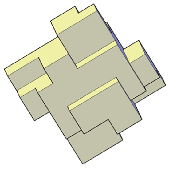
Figure 1.
MAYA block.
Easy to make: The formwork is made through superimposition in an ordered sequence of a plurality of square layers (six layers, as shown in Figure 2).
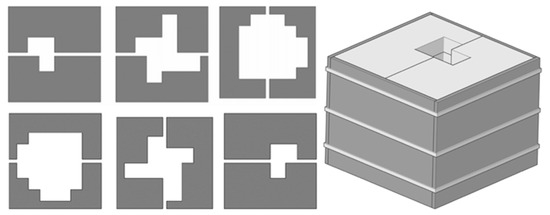
Figure 2.
MAYA mold.
The six square layers may be made by using simple and inexpensive manufacturing technologies. By way of example, and not by way of limitation, the square layers may be made of Styrofoam or polystyrene, and the four-side square panels may be optionally made of wood. The materials employed facilitate a reduction in the production prices of artificial units. In formwork construction, it is feasible to provide the end user with only the technical specifications, as the formwork can be constructed directly on site by non-specialized workers due to its simplicity. Moreover, the use of such materials allows, at the end of the manufacturing of the artificial units, the re-use of the formworks at the construction site for other necessary works and operations and may favor the complete environmental recycling of the materials, thus determining a further reduction in costs of both construction of the artificial units and the entire general project.
Easy to place: The artificial unit allows the installation operations to be carried out without requiring specialized personnel or high-tech instrumentation, achieving interlocking independent from the mutual placement of the units, favoring a random, not induced arrangement, achieving what is defined as mutual automatic interlocking. This implies that the positioning operations are expedited and streamlined, allowing for a reduction in construction time and, consequently, a decrease in costs related to equipment, staff, and operational phases for executing the project.
From the structural point of view, the configuration of the shape and its easy installation permit the artificial units to be arranged optimally, even in relation to the conditions of engagement, preventing the contiguous faces from coupling with each other, which is different from what occurs, for instance, for cubes. Thus, regardless of the precise arrangement of the individual units composing the layer, adequate roughness and porosity are consistently ensured, which mitigates the impact of wave motion on the structure’s exterior and improves energy dissipation (Figure 3).
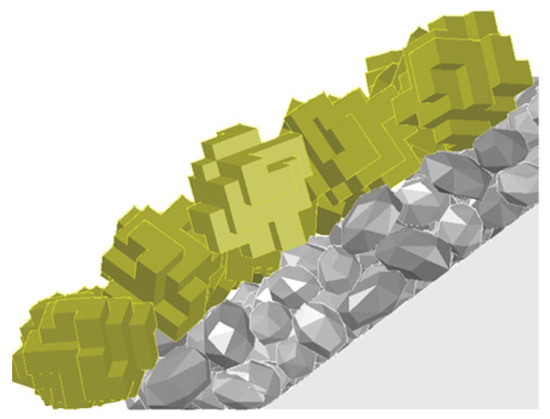
Figure 3.
MAYA in place.
Although a double-layer CAU is preferred by designers, a single layer was selected for this new development considering economic feasibility. It is a common perception that a double layer is generally much more stable than a single layer. The placement of single-layer blocks—such as ACCROPODE, CORE-LOC, and Xbloc—around curved or roundhead areas of a breakwater is complex, and their hydraulic stability is comparatively lower [13]. Consequently, the development of a new block with a simple layout seeks to overcome these construction limitations and facilitate a simpler process of assembly, as its formwork is easy to fabricate on site (Figure 2).
2.2. Scale Requirement and Scale Effect
Gravity forces predominate in free surface flow and thus most hydraulic models can be designed using the Froude criterion:
where
- L is a reference length [m];
- V is a reference velocity [m/s];
- g is the gravity acceleration [m/s2];
- m and p indices refer to the model and the prototype, respectively.
Based on the capacity of the wave flume and the wave maker, the model length scale factor has been chosen as 1/20, and consequently, the reduction scales of speed and time will be derived by the equations in Table 1:

Table 1.
Model scale factors.
2.3. Unit and Structure Design
Breakwater design employs semi-empirical formulas obtained from hydraulic model testing. Hudson (1959) [14] introduced a widely adopted expression to calculate the mass of armor units, based on experiments involving non-overtopped, permeable rock structures exposed to regular waves.
where
- W50 = Average unit weight;
- g = Gravity acceleration;
- ρr = Mass density of rocks;
- H = Characteristic wave height at the toe of the structure;
- KD = Stability coefficient;
- ∆ = Relative buoyant density ( − 1);
- α = Slope angle.
The stability coefficient KD is a dimensionless coefficient characteristic of the type of unit, the type of section (head or trunk of the structure), the number of armor layers, and the type of incident wave (whether breaking or non-breaking wave).
An intermediate value of KD, set at 5.0, has been assumed in comparison to the natural and Tetrapod blocks. Having set the density of the concrete to 2500 kg/m3, and knowing the slope of the structure (cotα = 4/3), the design wave height at the toe of the structure was set to Hs = 4 m (at prototype scale), so as to ensure a reserve of wave energy through which to increase the probability of failure of the structure.
With these parameters, using Formula (3), the average weight block was calculated as W = 69.935 N, corresponding to a nominal diameter Dn = 1.41 m (at prototype scale).
A length scale of 1:20 was applied for the breakwater model and the unit size was determined for the prototype (Table 2).
Table 2.
Armor unit specifications.
The model of a trunk breakwater section was created at a 1:20 scale (Froude analogy). It included a core material (quarry run), a double-layered underlayer, toe protection in natural stones, and armor with a Maya placement in a single random layer (Figure 4a–c). The toe protection was calculated in accordance with the Shore Protection Manual 1984 [15].
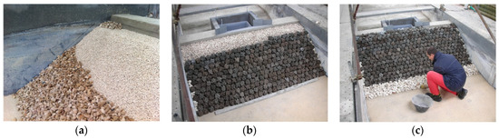
Figure 4.
Construction phases: (a) core and first layer of filter; (b) second layer of filter and armor layer; (c) toe protection.
The design of the layer of the structure is a function of the weight of the armor layer Warmor:
1/15 Warmour ≤ Wfilter ≤ 1/10 Warmour under layer
1/6000 Warmour ≤ Wcore ≤ 1/200 Warmour core
Wtoe-protection = 1/10 Warmour toe protection
This corresponds to the following dimensions (Table 3) when the stone material is used:
Table 3.
Properties of used natural stones.
On the front slope, a value of 4:3 was adopted to study the structure in the most unfavorable conditions for hydraulic stability.
The width of the berm corresponding to 3 stones in size (frequently adopted solution for this kind of structure) was chosen, while the height was chosen at 3.00 m m.s.l. for the prototype scale. In the rear part of the breakwater, a total closure by means of a crown wall at the same height of the berm was operated (Figure 5).
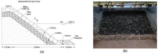
Figure 5.
Rubble mound breakwater: (a) model section; (b) physical model.
2.4. Facilities of Physical Model Experiments
The experimental study, reproduced at a 1:20 Froude scale, was performed in the wave flume of the Research and Experimentation for Coastal Defense Laboratory (LIC) of the Department of Civil, Environmental, Territorial, Building Engineering and Chemistry (DICATECh) of the Technical University of Bari (Figure 6a).
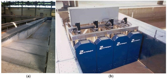
Figure 6.
Equipment of LIC: (a) wave flume; (b) wave maker.
The channel measures 50.00 m in length, 2.50 m in width, and 1.20 m in height. Wave attacks were generated based on JONSWAP spectra using a wave maker positioned at the end of the flume, developed by HR Wallingford (Howbery Park, Wallingford, Oxfordshire, UK), which includes four blades, each 0.6 m wide (Figure 6b).
In the rear part of the generator, a cliff was created for the absorption of the energy of the waves transmitted backwards by the movement of the blades, in order to avoid reflection but, above all, to preserve the integrity of the equipment (Figure 7).
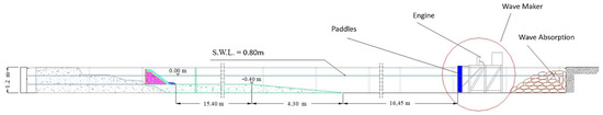
Figure 7.
Schematization of a flume.
Water surface oscillation was recorded by an array of 5 resistive wave gauges installed along the wave flume during the tests. One resistive wave gauge was placed 24 m from the offshore toe of the breakwater to verify generated waves; a group of three probes was positioned near the breakwater toe to apply the standard reflection analysis; and a run-up meter, displaced along the structure, measured the up/down-rush processes along the front slope (Figure 8).
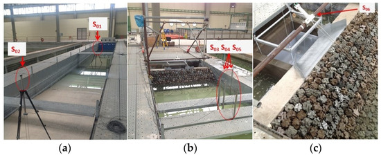
Figure 8.
Probe positions in the channel: (a) wave generation; (b) wave reflection; (c) wave run-up.
This study was developed with a channel represented in Figure 9, characterized by a depth of (16 m in prototype scale—80 cm in model scale). This phase was designed to study the reflection, run-up, and overtopping phenomena under breaking waves.
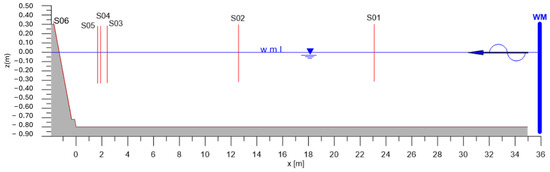
Figure 9.
Physical flume configuration and probe positions.
2.5. Numerical Modeling
The numerical flume has been set up at full scale and reproduces both the structure and foreshore without distortion.
The first important step of the analysis is the definition of the breakwater section, both with concrete units and geometrical properties in accordance with a realistic prototype structure placement, as discussed in [8].
First, the inner impermeable section (including the core) is designed. Then, on its slope facing the sea, a double filter layer (in virtual stones or blocks, weighing 1000–3000 kg) is modeled by digitally overlapping the individual elements one by one according to the real geometry.
The definition of the breakwater is then completed by introducing, with the same digital technique, a single armor layer in Maya, and then with other blocks tested.
Once the geometry is fully defined, it is imported into the CFD code to evaluate the hydrodynamic interactions. This is possible with the distinguishing features of FLOW-3D HYDRO 2024R1®, such as the FAVOR™ (Fractional Area Volume Obstacle Representation) method, which is used to define complex geometric regions within rectangular grids and multi-block meshing. FAVORTM is a very powerful method for incorporating geometry effects into the governing equations. The methodology and the use of Computational Fluid Dynamics (CFD) for coastal engineering studies are well-documented in the literature, as indicated in references [16,17,18].
The computational domain is divided into four zones with two sub-domains with different grid sizes (Figure 10) selected after the grid sensitivity study.
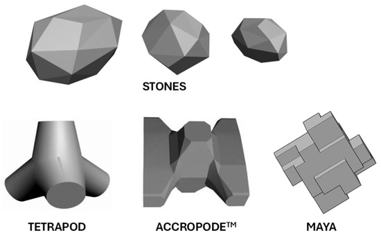
Figure 10.
Three-dimensional virtual block.
Three uniform grids were implemented: ∆x = ∆y = ∆z = 0.3, ∆x = ∆y = ∆z = 0.2, and ∆x = ∆y = ∆z = 0.15.
To measure the degree of convergence, two indicators were used:
- The “relative error” from the wider to the finer grid, defined as:where F represents the force signal and the subscripts “wide” and “fine” refer to the wider and finer grids used. The symbol “Stdev” indicates standard deviation.
- The square correlation between the wave signals at the toe of the structure:
Results of the analysis are summarized in Table 4, which confirms the substantial coherence between the grids 0.2 m × 0.2 m × 0.2 m and 0.15 m × 0.15 m × 0.15 m in size (R2 is around 99%).
Table 4.
Indicator for grid sensitivity study.
Accordingly, ∆x = ∆y = ∆z = 0.2 m was selected for the local mesh (mesh 1, on breakwater); while the general mesh size (mesh2) for all the computations was chosen to be 0.50 × 0.50 × 0.20 m; this allowed it to save computational time (reducing the total count of cells) while maintaining adequate vertical resolution both in the wave generation zone and along the structure (Figure 11).

Figure 11.
Regions of the computational domain with different grid sizes.
Following the experimental model scale and developed in the laboratory, as discussed previously, the length of the wave generation zone (W.G. zone) and wave removal zone (W.R. zone) is 700 m in the X direction, 5 m in the Y direction, and 25 m in the Z direction. The still water level (d) is 10.00 m; the wave structure interaction zone (W.S.I. zone) and the structure’s geometry remain consistent with the details provided in the previous paragraph and are executed at prototype scale. A damping zone defined by a special geometry component, properly dimensioned as a function of a wavelength, called a wave absorber, is added in the numerical domain. It is completely open to fluid flow but applies damping to wave motion. The damping coefficient increases linearly in the wave propagation direction from 0 to 1.0 s −1 in the sponge layer according to developer of the Flow3D HYDRO 2024R1® software.
The boundary conditions have been applied at the side of the 3D numerical domain. On the right side, a condition of pressure “P” is applied that allows fluid to outflow but with specific distribution; this is necessary to keep a constant fluid level in the flume during long-time simulation. The waves are generated through the mass source with a specific conversion of spectral parameters into the volume flow rate.
The random waves (Jonswap spectrum shape) have been generated from a solid element, located below the still water level.
From it, a flow has been introduced according to mass source theory [19].
where s(x,y,t) is the nonzero mass source function within the source region .
Inverse Fourier transformation can reconstruct a wave train from a known energy spectrum of an irregular wave train by superposing a finite number of wave modes from i = 1 to n
where φi is the phase of the i-th wave mode and ωi is the wave frequency.
An example of mass source flow rate is shown in Figure 12.
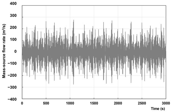
Figure 12.
Example of mass source flow rate.
Comparing the numerical results against known analytical solutions is a preliminary validation of the procedure implemented (Figure 13 and Figure 14).
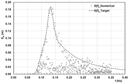
Figure 13.
Example validation of wave spectrum generated with mass source.
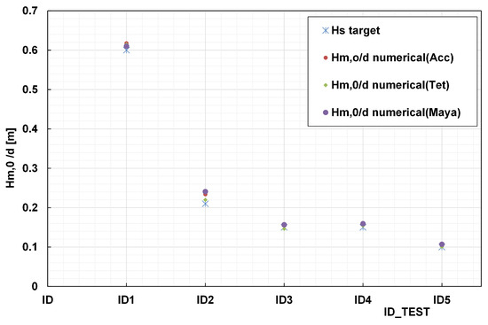
Figure 14.
Validation of Hm,0/d generated with mass source for all numerical simulations.
On the bottom, the condition of wall ‘‘W’’ was applied, and lateral and upper symmetry (S) were selected.
Fluid properties were set by loading through a Fluids Database, the water at 20 °C was selected for the experiments. Turbulence was simulated using the RNG model and the main parameters are summarized in Table 5.
Table 5.
General parameter settings in numerical study.
The RANS equations that govern the problem are resolved by Flow3D HYDRO 2024R1® using a staggered grid finite difference scheme, while the free surface is tracked using the Volume of Fluid (VOF) technique. The software maintains the stability and accuracy of the solution by implementing a variable time step. This approach complies with the Courant–Friedrichs–Lewy (CFL) stability criterion and ensures that surface waves are unable to propagate more than one cell per time step.
Wave Conditions
In order to analyze the numerical wave interaction with a new concrete armor unit, five simulations have been carried out with different wave characteristics and a wide range of Iribarren Numbers (Table 6).
Table 6.
Wave parameters tested in the experimental model vs. the numerical model.
Irregular waves are generated according to a JONSWAP spectrum (γ = 3.3) with significant wave heights from 1.00 to 6.00 m and peak periods from 7.6 to 20.00 s (Table 2). The length of irregular wave trains is determined to include at least 500 waves. The influence of the test duration on the overtopping variability has been investigated by [20], who, by performing a sensitivity analysis on the partial overtopping time series, have pointed out that shorter time series (e.g., 500 waves) can be used for overtopping tests obtaining the same order of accuracy with respect to the longer ones (e.g., the recommended 1000 waves).
Table 6 shows the experimental and numerical ranges that were tested to investigate the configuration considered for a wide range of incident wave conditions.
3. Results
3.1. Influence of Number of Waves on Numerical Wave Reflection
In order to quantify the influence of the number of waves on the stability of numerical simulation and the influence on main characteristics, aiming both at obtaining robust quantity estimates and at minimizing the experiment duration, an error analysis has been carried out. The parameter εN that describes the relative error between Kr,Nw, and Kr,500 has been defined as follows:
where Kr,500 is the reflection coefficient obtained by using the time series with Nw = 500 and Kr,Nw is the reflection coefficient obtained by using partial overtopping time series that contain Nw (i.e., 100 ≤ Nw ≤ 500). When εN = 0, the whole time series and the partial ones provide identical results.
The same approach was used for incident wave height:
The results of the error analysis are shown in Figure 15 and Figure 16; each panel refers to a different value of the relative wave depth.
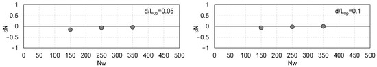
Figure 15.
Mean error εN of Kr as a function of the considered number of waves per test Nw.
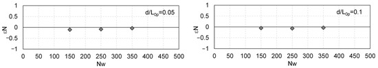
Figure 16.
Mean error εN of H,si as a function of the considered number of waves per test Nw.
As expected, εN is larger for small values of Nw. Note that the larger value of error for the lower values of relative water depth can be explained by the long period carried out in this range that influenced the performance of the wave absorber and consequently the stability of the simulation for a short number of waves.
3.2. Numerical and Experimental Wave Reflection
The numerical results were qualitatively compared to the database that was available from previous studies.
In Pratola et al., 2021 [21], an extensive analysis of the wave reflection coefficient was carried out. The experimental data results of Kr have been compared with different parameters such as peak period, the surf similarity parameter, wave steepness, and relative water depth.
According to [21], the numerical reflection coefficient has the same trend found for the experimental data. The initial comparison of findings demonstrates a strong correlation between the numerical and experimental models, as shown in Figure 17.

Figure 17.
Validation of the numerical reflection coefficient Kr.
Several studies have dealt with the testing of the Muttray et al. [22] formula by changing experimental conditions. In particular, Calabrese et al. [23] carried out tests with the ECOPODESTM armored RMB with two different front slopes: (i) a slope of 2:3 (same as the Muttray et al. experiments [22]) and (ii) a slope of 3:4 (equal to that in the present paper).
Figure 18 shows the comparison of the present numerical and experimental results with the curves by Buccino et al. [24] with a slope of 3:4 (named as “B 3:4”)
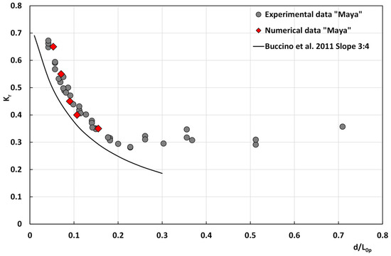
Figure 18.
Reflection coefficient related to d/L0p [24].
The figure also shows that the reflection coefficient is not influenced by d/L0p for values (of the relative water depth) greater than 0.25.
Like Buccino et al. [24]’s development for ECOPODES, Pratola et al., 2021 [21] further refined the estimation of the A (m) and B (m) coefficients of the Muttray et al. formula, providing new values (Table 7).
Table 7.
New coefficients A (m) and B (m) to be included in Muttray equation refitted to exploit experimental and numerical data.
These coefficients were estimated to fit the experimental data of Kr, obtaining the best values of the coefficient of determination (R2) and standard deviation (σ) between measured and predicted Kr.
The structure that was evaluated appears to have a higher reflection coefficient than the rubble mound breakwater that was tested by Buccino et al. [24]. The presence of the seawall behind the rubble mound structure, the (bulk) permeability, and the novel concrete unit are likely the reasons for this result.
Additionally, it should be noted that the numerical model yields satisfactory accuracy results.
Comparison of the Hydrodynamic Characteristics of Maya with Different Armor Blocks
Diaz-Carrasco et al. [25] proposed a new formula to estimate Kr in a wider range of variations in the relative water depth. The reflection coefficients (Equation (13)) are estimated to exploit a sigmoid function depending on the relative water depth and front slope d/(L tan α):
The Kr data observed in the experimental tests carried out in this work were then used to fit Equation (13). The values of the refitted coefficients are shown in Table 8.
Table 8.
Values of the sigmoid function parameters refitted for the Maya unit and 3:4 front slope.
Numerical experiments are also conducted to evaluate the proposed formula for other armor blocks, including the Tetrapod and AccropodeTM (Figure 19). The volume of the armor unit is 8 m3 (weight of 20 ton) for Tetrapod placed in a double layer and 6 m3 (14 ton) for AccropodeTM placed in a single layer. The porosity parameter p is 0.5 and 0.53, respectively. The breakwater has a slope of 4/3.
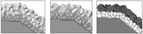
Figure 19.
Numerical virtual structures.
The refitting developed for experimental data of the maya block is also validated with the numerical data of three different blocks.
The performance of the Diaz-Carrasco formula refitted with experimental data is evaluated with numerical results of Maya and other blocks. A good agreement (R2 equal to 0.995) is shown in Figure 20.
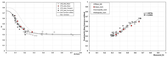
Figure 20.
Numerical result validation of wave reflection.
Figure 20 illustrates that Maya’s performance is comparable to that of AccropodeTM, which exhibits comparable behavior. Even though the Tetrapod is constructed in two layers, it provides a minor value of wave reflection.
In [21] the reflection coefficient was proposed to be estimated by a power law as follows:
where the parameters were estimated by means of a non-linear least square method: C = 0.1381 (with a 0.95 confidence interval ±0.020), a = −0.1810 (with a 0.95 confidence interval ±0.104), and b = 0.5035 (with a 0.95 confidence interval ±0.162).
Equation (14) was tested against other widely used formulas for the estimation of the reflection coefficient, which considers the dependence of Kr from the surf similarity parameter ξm-1,0 [25,26] and the relative water depth [27]. The numerical results are added in Figure 21, which shows a satisfactory agreement between the experimental points and those calculated using Equation (14).
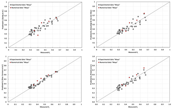
Figure 21.
Comparison of predicted and measured reflection coefficients.
To evaluate the accuracy of the predictive models, some indicators have been calculated. The mean squared error, mean absolute error, root mean squared error, and R-squared or coefficient of determination metrics are used to evaluate the performance of the model in regression analysis.
The agreement is also confirmed by the accuracy assessment estimated using the statistical parameters reported in Table 9.
Table 9.
Estimated best-fit values for the proposed approach and the existing formulations for experimental and numerical Maya results.
A lower value of MAE implies a higher accuracy of a regression model. However, a higher value of R-squared is considered desirable.
MAE is the mean absolute error, which is more robust to outliers than the MSE, which gives more importance to the highest errors; thus it is more sensitive to outliers. The NSE is defined as the ratio of the mean square error to the variance in the observed data, which is subtracted from unity and ranges from minus infinity to 1.0. Ritter and Munoz-Carpena [28] have proposed four model performance classes: unsatisfactory (NSE ≤ 0.65), acceptable (NSE = 0.65–0.8), good (NSE = 0.8–0.9), and very good (NSE ≥ 0.9). This is due to the fact that the agreement is improved as the NSE values increase.
Nevertheless, the numerical approach is employed to compare the same configuration with other blocks (Acropode and Tetrapod).
The data set consists of 15 observations, and the statistical parameters are reported in Figure 22 and Table 10.
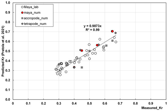
Figure 22.
Comparison of measured and predicted reflection coefficients (data from [21]).
Table 10.
Estimated best-fit values for the proposed approach and the existing formulations for numerical and experimental results for all types of blocks.
The formula that was proposed proved to be effective when tested with other blocks. Nevertheless, Diaz’s formula continued to be the most effective.
3.3. Run-Up and Overtopping
In the case of random wave attacks, unlike in the case of the present work, every single wave produces a different run-up value due to the stochastic nature of the incident waves. Thus, the need to define a representative value of the phenomenon was born.
The characteristic run-ups that are used most frequently in the formulations present in the literature are the 2% run-up (Ru2%) and the 10% run-up (Ru10%), defined, respectively, as the run-up that is exceeded by 2% and 10% of the accident waves at the foot of the structure.
Generally, the formulas that are defined for the run-up prediction are empirical, drawn from experimental studies conducted on physical models.
Normally, the run-up is adimensionalized with the wave height incident on the structure. As a phenomenon closely linked to the slope of the structure and to the characteristics of the incident wave, the most representative parameter which it is put in relation to is the surf similarity parameter.
For the run-up measurement, a resistive probe was used. The probe was positioned along the structure, as can be seen in Figure 23 where the probe and the water tank for wave overtopping measurement is clearly visible.

Figure 23.
Probes along the armor surface to estimate the wave run-up (sx). Tank overtopping system in experimental analysis (dx).
The numerical and experimental values are consistent with the literature values (Figure 24). Furthermore, it is worth noting that the Maya block exhibits lower run-up values than the literature curves for the permeable layer. This is due to the combined effects of high porosity and high friction.

Figure 24.
Correlations between Eurotop Manual 2018 graph and experimental and numerical data of run-up 2% (adapted by [29]).
The MAYA boulder demonstrated better results regarding this hydrodynamic parameter when compared to the other units.
Even though the Maya boulder is an armored unit that is intended to be positioned in a single layer, the run-up rate of the Maya was found to be comparable to that of the Tetrapod (double layer) throughout the spectrum of the realistic wave and geometric conditions that were tested. This finding implies that layer thickness is comparatively less significant than surface roughness and porosity.
The graph in Figure 25 includes the wave overtopping values that were measured in MAYA experiments. In the same graph, solid symbols are used to distinguish structures that are constituted by a single layer, such as Accropode, Core-loc, Xbloc, and cubes, from those that are composed of a double layer, which are represented with empty symbols.
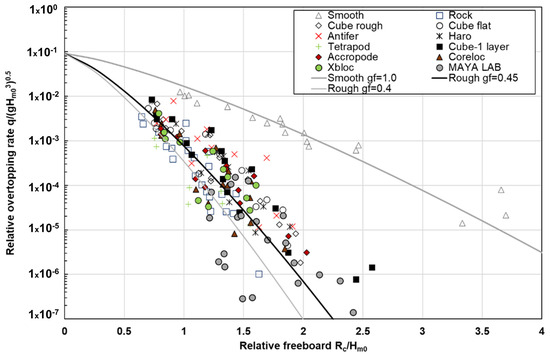
Figure 25.
Overtopping data validation (data from Eurotop Manual 2018 [29]).
The experimental points depicted in the graph are well-placed within the band surrounding the characteristic curve of Eurotop Manual 2018 [29].
The experimental data indicate a consistently reduced flow rate in comparison to the characteristic points associated with tests performed using other block types.
3.4. Roughness Factor for Maya Block
The analysis also shows the influence of roughness factors. The overtopping rates on a rubble mound breakwater depend on structural and environmental conditions.
Bruce et al., 2009 [30] conducted experiments to determine the roughness factor for inclined sloped structures constructed with natural boulders and various cladding units in non-breaking wave conditions. For structures with a face slope of 1:1.5 and a ridge width of 3Dn, overtopping was measured. In Figure 26, the aforementioned results are summarized in a graph that displays two lines adjacent to the characteristic points of the various structures. The upper line corresponds to smooth paraments, as determined by the Van der Meer 2002 [31] equation: γf = 1.0. The lower line, which corresponds to breakers with revetments composed of natural rocks, was determined by the same equation, which placed γf = 0.45. This second line is representative of a mean value among those characteristics of the different armor units analyzed but clearly shows the effect of roughness on the phenomenon of overtopping.
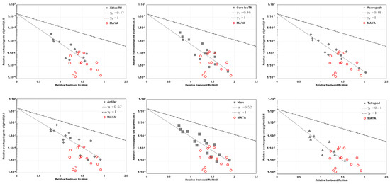
Figure 26.
Overtopping performance of different armor units for rubble mound breakwaters (data from Bruce et al., 2009 [30]).
It is evident that, under identical overtopping conditions, constructions composed of natural boulders require just half the crowning portion compared to those with smooth facings.
In order to compare the run-up values measured on the model with the values computed using the formula, different values for the roughness coefficient γf were assigned to optimize the trend line of the Maya points, hence maximizing R2.
As shown in Figure 27, with a roughness value of 0.4, the data show a good fit.

Figure 27.
Comparison of experimental and empirical values of run-up 2%.
It is possible to observe that Maya presents a value of γf between the lowest values when we compare the aforementioned values with those in Table 11, which refers to structures with a shoe of 1:1.5 and relative armor blocks that are currently commonly used in the field of marine engineering and to be positioned in double layer.
Table 11.
Roughness coefficient for different armor layer blocks (data from [31]).
The roughness coefficient for the Maya block was approximately 0.40.
4. Discussion and Conclusions
This paper has discussed results from an experimental investigation of a new concrete armor unit MAYA conducted at LIC Laboratory of the DICATECh Department of the Technical University of Bari.
The experimental test was designed to examine wave reflection, run-up, and overtopping. The hydraulic response of debris mound breakwaters armored with Maya units has been presented, and a numerical investigation with an innovative procedure has been addressed. Additionally, the capabilities of the Maya block were evaluated against a numerical testing campaign conducted using armored buildings employing commercially available blocks widely used in coastal engineering (e.g., Tetrapod and AccropodeTM).
The main conclusions of the work can be strictly synthesized as follows:
The shape and the size of the amour voids, as well as the roughness of the units, would lead to a significant reduction in both reflexivity and run-up height compared to rocky structure.
A novel empirical formulation was proposed with the following features: The fitting procedure confirmed that both of the dimensionless parameters (surf similarity parameter and relative water depth) cannot be neglected in the case at hand. Moreover, the implementation of a novel numerical model supported the findings acquired during the experimental phase.
The results of this model were compared to those of previous estimation formulas under the same conditions. Low data dispersion and relatively high error were found but were of a similar order to those observed in previous studies. In conclusion, the proposed model in a previous study was capable of estimating wave reflection from a rubble mound breakwater with a new type of block at an acceptable level of accuracy. The power of the equation derived in [19] has been confirmed for numerical results of different types of armor blocks.
The processes related to flow–structure interaction are examined using Numerical Navier–Stokes models, in addition to turbulence modeling and Volume of Fluid surface tracking methods (known as RANS/VOF). The equations included in the model facilitate the simulation of intricate three-dimensional flows, encompassing highly non-linear waves, wave breaking, and porous flow. A virtual structure is constructed by overlapping individual 3D elements, like real construction practices, and a sufficiently fine numerical grid is applied to assess the flow in the interstices between the blocks. This capability results from the integration of three-dimensional CAD models with increasingly sophisticated numerical resolution software. The implementation of a novel and robust treatment for wave generation and reflection has demonstrated that this numerical method is an effective tool for analyzing the hydraulic responses of coastal defense systems.
This investigation allowed the assessment of the roughness factor of the MAYA block.
Finally, it is feasible to deduce that the new block exhibits potential in the field of coastal engineering due to its exceptional hydraulic performance and reduced construction costs.
Author Contributions
Conceptualization, A.D.L., F.D. and. L.P.; methodology, A.D.L., F.D. and L.P.; software, A.S.; validation, A.D.L., A.S. and L.P.; formal analysis, A.S. and L.P.; investigation, L.P.; resources, F.D. and L.P.; data curation, L.P. and A.S.; writing—original draft preparation, A.D.L.; writing—review and editing, F.D. and V.P.B.; visualization, F.D. and V.P.B.; supervision, F.D. All authors have read and agreed to the published version of the manuscript.
Funding
This research received no external funding.
Data Availability Statement
To gain access to the experimental data, please contact the authors.
Conflicts of Interest
The authors declare no conflicts of interest.
References
- Khan, M.; Behera, H.; Sahoo, T.; Neelamani, S. Boundary element method for wave trapping by a multi-layered trapezoidal breakwater near a sloping rigid wall. Meccanica 2021, 56, 317–334. [Google Scholar] [CrossRef]
- Khan, M.; Behera, H. Analysis of Wave Action Through Multiple Submerged Porous Structures. J. Offshore Mech. Arct. Eng. 2020, 142, 011101. [Google Scholar] [CrossRef]
- Vicinanza, D.; Cáceres, I.; Buccino, M.; Gironella, X.; Calabrese, M. Wave disturbance behind low crested structures: Diffraction and overtopping effects. Coast. Eng. 2009, 56, 1173–1185. [Google Scholar] [CrossRef]
- Calabrese, M.; Vicinanza, D.; Buccino, M. 2D wave set up behind low crested and submerged breakwaters. In Proceedings of the 13th International Conference ISOPE, Honolulu, HI, USA, 25–30 May 2003; ISOPE: Cupertino, CA, USA, 2003. ISBN 1-880653-60-5. [Google Scholar]
- Calabrese, M.; Buccino, M.; Pasanisi, F. Wave breaking macrofeatures on a submerged rubble mound breakwater. J. Hydro-Environ. Res. 2008, 1, 216–225. [Google Scholar] [CrossRef]
- Dentale, F.; Donnarumma, G.; Pugliese Carratelli, E. Wave Run Up and Reflection on Tridimensional Virtual Breakwater. J. Hydrogeol. Hydrol. Eng. 2012, 1, 1–8. [Google Scholar] [CrossRef]
- Altomare, C.; Gironella, X.F.; Crespo, A.J.F.; Domìnguez, J.M.; Gòmez-Gesteira, M.; Rogers, B.D. Improved Accuracy in Modelling Armoured Breakwaters with SPH. In Proceedings of the 7th International SPHERIC Workshop, Prato, Italy, 29–31 May 2012; pp. 1–8. Available online: http://hdl.handle.net/2117/20630 (accessed on 26 September 2012).
- Di Leo, A.; Reale, F.; Dentale, F.; Viccione, G.; Carratelli, E.P. Wave-structure interactions a 2d innovative numerical methodology. In Proceedings of the 23rd Conference of the Italian Association of Theoretical and Applied Mechanics, Salerno, Italy, 4–7 September 2017; Volume 2, pp. 1699–1708. [Google Scholar]
- Viré, A.; Xiang, J.; Milthaler, F.; Farrel, P.E.; Piggott, M.D.; Latham, J.P.; Pavlidis, D.; Pain, C. Modelling of fluid-solid interactions using an adaptive mesh fluid model coupled with a combined finite-discrete element model. Ocean. Dyn. 2012, 62, 1487–1501. [Google Scholar] [CrossRef]
- Latham, J.P.; Anastasaki, E.; Xiang, J. New modelling and analysis methods for concrete armour unit systems using FEMDEM. Coast. Eng. 2013, 77, 151–166. [Google Scholar] [CrossRef]
- Milanian, F.; Niri, M.Z.; Najafi-Jilani, A. Effect of Hydraulic and structural parameters on the wave run-up over the berm breakwaters. Int. J. Nav. Archit. Ocean. Eng. 2017, 9, 282–291. [Google Scholar] [CrossRef][Green Version]
- Liang, B.; Ma, S.; Pan, X.; Lee, D.Y. Numerical Modelling of Wave Run-up with Interaction Between Wave and Dolosse Breakwater. J. Coast. Res. 2017, 79, 294–298. [Google Scholar] [CrossRef]
- Jensen, O.J. Safety of breakwater armour layers with special focus on monolayer armour units. In Proceedings of the Coasts, Marine Structures and Breakwaters, Edinburgh, UK, 17–20 September 2013. [Google Scholar]
- Hudson, R.Y. Laboratory Investigation of Rubble-Mound Breakwaters. J. Waterw. Harb. Div. 1959, 85, 93–121. [Google Scholar] [CrossRef]
- Shore Protection Manual. Coastal Engineering Research Center. Department of the Army. Waterways Experiment Station, Corps of Engineers, Vicksburg, MS, USA. 1984. Available online: https://usace.contentdm.oclc.org/digital/collection/p16021coll11/id/1933 (accessed on 25 October 2025).
- Buccino, M.; Daliri, M.; Dentale, F.; Di Leo, A.; Calabrese, M. CFD experiments on a low crested sloping top caisson breakwater. Part 1. nature of loadings and global stability. Ocean Eng. 2019, 182, 259–282. [Google Scholar] [CrossRef]
- Di Leo, A.; Buccino, M.; Dentale, F.; Pugliese Carratelli, E. CFD Analysis of Wind Effect on Wave Overtopping. In Proceedings of the 32nd International Ocean and Polar Engineering Conference, Shanghai, China, 5–10 June 2022. [Google Scholar]
- Tuozzo, S.; Di Leo, A.; Ciccaglione MCDentale, F.; Cordova Lopez LCalabrese, M.; Buccino, M. Vertical Seawalls Protected by Rubble Mound Structures: Prediction Tools and Physical Insight. In Proceedings of the Coastal Engineering Conference, Rome, Italy, 8–15 September 2023. [Google Scholar]
- Lin, P.; Liu, P.L.F. Internal wave-maker for navier-stokes equation models. J. Waterw. Port Coast. Ocean. Eng. 1999, 125, 207–215. [Google Scholar] [CrossRef]
- Romano, A.; Williams H, E.; Bellotti, G.; Briganti, R.; Dodd, N.; Franco, L. About some uncertainties in the physical and numerical modeling of wave overtopping over coastal structures. Coast. Eng. Proc. 2014, 1, structures.71. [Google Scholar] [CrossRef]
- Pratola, L.; Rinaldi, A.; Molfetta, M.G.; Bruno, M.F.; Pasquali, D.; Dentale, F.; Mossa, M. Investigation on the Reflection Coefficient for Seawalls Protected by a Rubble Mound Structure. J. Mar. Sci. Eng. 2021, 9, 937. [Google Scholar] [CrossRef]
- Muttray, M.; Oumeraci, H.; Oever, E.T. Wave reflection and wave run-up at rubble mound breakwaters. Coast. Eng. 2007, 4314–4324. [Google Scholar] [CrossRef]
- Calabrese, M.; Buccino, M.; Ciardulli, F.; Di Pace, P.; Tomasicchio, R.; Vicinanza, D. Wave run-up and reflection at rubble mound breakwaters with ecopode armor layer. Coast. Eng. Proc. 2011, 1, structures.45. [Google Scholar] [CrossRef]
- Buccino, M.; Calabrese, M.; Ciardulli, F.; Di Pace, P.; Tomasicchio, G. One layer concrete armor units with a rock-like skin: Wave reflection and run-up. J. Coast. Res. 2011, 64, 469–473. [Google Scholar]
- Díaz-Carrasco, P.; Eldrup, M.R.; Andersen, T.L. Advance in wave reflection estimation for rubble mound breakwaters: The importance of the relative water depth. Coast. Eng. 2021, 168, 103921. [Google Scholar] [CrossRef]
- Zanuttigh, B.; van der Meer, J.W. Wave reflection from coastal structures in design conditions. Coast. Eng. 2008, 55, 771–779. [Google Scholar] [CrossRef]
- Seelig, W.N.; Ahrens, J.P. Estimation of Wave Reflection and Energy Dissipation Coefficients for Beaches, Revetments, and Breakwaters; Technical Paper 81-1; Coastal Engineering Research Center: Fort Belvoir VA, USA, 1981. [Google Scholar]
- Ritter, A.; Muñoz-Carpena, R. Performance evaluation of hydrological models: Statistical significance for reducing subjectivity in goodness-of-fit assessments. J. Hydrol. 2013, 480, 33–45. [Google Scholar] [CrossRef]
- Van der Meer, J.W.; Allsop, N.W.H.; Bruce, T.; De Rouck, J.; Kortenhaus, A.; Pullen, T.; Schüttrumpf, H.; Troch, P.; Zanuttigh, B. EurOtop. Manual on Wave Overtopping of Sea Defences and Related Structures. 2nd Edition. 2018. Available online: www.overtopping-manual.com (accessed on 9 July 2025).
- Bruce, T.; van der Meer, J.W.; Franco, L.; Pearson, J.M. Overtopping performance of different armour units for rubble mound breakwaters. Coast. Eng. 2009, 56, 166–179. [Google Scholar] [CrossRef]
- TAW. Technical Report on Wave Run-Up and Wave Overtopping at Dikes; Van der Meer, J.W., Ed.; Technical Advisory Committee on Flood Defence: Delft, The Netherlands, 2002; Available online: https://www.overtopping-manual.com/assets/downloads/TRRunupOvertopping.pdf (accessed on 26 October 2025).
Disclaimer/Publisher’s Note: The statements, opinions and data contained in all publications are solely those of the individual author(s) and contributor(s) and not of MDPI and/or the editor(s). MDPI and/or the editor(s) disclaim responsibility for any injury to people or property resulting from any ideas, methods, instructions or products referred to in the content. |
© 2025 by the authors. Licensee MDPI, Basel, Switzerland. This article is an open access article distributed under the terms and conditions of the Creative Commons Attribution (CC BY) license (https://creativecommons.org/licenses/by/4.0/).