Article

Calculating the Sediment Flux in Hydrometric Data-Scarce Small Island Coastal Watersheds

1
Hainan Key Laboratory of Marine Geological Resources and Environment, Hainan Marine Geological Survey Bureau, Haikou 570206, China
2
College of Electronic and Information Engineering, Guangdong Ocean University, Zhanjiang 524088, China
3
Guangdong Provincial Key Laboratory of Intelligent Equipment for South China Sea Marine Ranching, Zhanjiang 524088, China
4
Hainan Geology Detection and Research Centre, Haikou 570206, China
5
Marine Geological Institute of Hainan Province, Haikou 570206, China
*
Authors to whom correspondence should be addressed.
J. Mar. Sci. Eng. 2025, 13(11), 2039; https://doi.org/10.3390/jmse13112039
Submission received: 16 August 2025 / Revised: 9 October 2025 / Accepted: 21 October 2025 / Published: 24 October 2025
(This article belongs to the Special Issue Coastal Geochemistry: The Processes of Water–Sediment Interaction)

Abstract

The information of sediment flux (Qs) from hydrometric data-scarce small coastal watersheds is an important supplement for interpreting the sedimentary records of continental shelf sedimentary systems. This paper proposes a solution to estimate their values based upon the empirical formula of small and medium-sized coastal watersheds in adjacent regions, taking the 25 small rivers in Hainan Island as example. Three categories of methods were applied to calculate the Qs. The first category involves the direct application of global empirical formulas, while the second and third categories utilizes empirical formulas that have been calibrated with regional characteristic data. The Qs calculation accuracy the above methods was validated by the observed values of typical rivers. Key findings include: (1) The area values of watersheds extracted from SRTM (Shuttle Radar Topography Mission) data exhibit a high correlation with actual values, confirmed the reliability and applicability of SRTM data; (2) The Global equation significantly overestimates Qs for the validation rivers (average relative error of 18.73), while employing the pristine-modified and disturbed-modified equations effectively improves the calculation accuracy (average relative errors of 0.72 and 1.64, respectively); (3) By averaging the results of different models, the Qs for the major rivers in Hainan Island was calculated as 6.07 Mt/a before large-scale human activities and 4.56 Mt/a after. This study demonstrates that modification not only needs to be considered to adjust global empirical formulas but also to differentiate between the scenarios of before and after large-scale human activities in small coastal watersheds.

1. Introduction

Riverine sediment flux (Qs) to the ocean serves as the fundamental material basis for the formation and development of continental shelf depositional systems [1,2]. It plays a crucial role not only in the cycling, transformation, and preservation of materials, energy, and information [3,4], but also directly or indirectly influences coastal biological and biogeochemical cycles [5]. A substantial body of research indicates that the Qs contributions from global small sized rivers, particularly certain mountainous torrential rivers in low-latitude regions, may exert greater impacts on the coastal zone than those from the world’s major large river systems [6,7]. Compared to large rivers, they often exhibit characteristics such as instantaneous large discharge, rapid material turnover, heightened susceptibility to extreme events and human activities and greater sensitivity to environmental changes [8]. Therefore, conducting systematic research on the small rivers Qs is of significant importance for better understanding the river basin-to-estuary material cycling processes driven by both natural and anthropogenic factors, and for achieving sustainable development, reliable disaster assessment, and prevention in estuarine and coastal regions.
Three methods are commonly used to obtain Qs: the watershed erosion rate estimation method [9,10], the calculation method based on hydrological observation data from estuaries [11], and the empirical formula method for river hydrological stations [8,12]. The first method often results in overestimations, as some sediment remains trapped within the watershed and does not fully reach the estuary [13]. The second one is the most accurate for obtaining Qs; however, it is not recommended for analyzing long-term flux issues due to the high costs associated with field observations and the limited temporal scope of the data [14]. The third one is frequently employed for discussions on annual or longer time scales [13,15]. It is primarily based on observational data from hydrological stations near the mouths of hundreds of rivers worldwide, along with environmental background parameters of their respective watersheds to construct semi-empirical estimation formulas [8,16,17,18]. However, multiple studies have indicated that these global estimation models can yield both overestimations [19] and underestimations [20,21] when applied to small and medium-sized rivers in Southeast Asia. Therefore, there is an urgent need to conduct case studies on the modification of empirical formulas to figure out whether the calibrated equations significantly improve prediction accuracy compared to global models.
This study addresses the significant discrepancies observed when applying existing global empirical formulas to calculate Qs from medium and small rivers into the sea. The focus is on the small rivers of Hainan Island as a representative research area. We quantify the calculation deviations of Qs into the sea for different rivers in the study area using various empirical formulas, and analyze the causes of these estimation discrepancies along with targeted correction strategies.

2. Materials and Methods

2.1. Study Area Description

Hainan Island located in the northern South China Sea. With a total area of 33,920 km2, it is China’s second-largest island after Taiwan Island (Figure 1a). Its topography is characterized by a central highland with Wuzhi Mountain (1867 m) as the uplift core, gradually descending toward the periphery, forming a radial pattern of high center and low surroundings (Figure 1b). The bedrock primarily consists of Paleozoic metamorphic and sedimentary rocks, later intruded by Mesozoic granites, and the northern outcrops are mainly composed of Cenozoic to Holocene volcanic rocks and basalts [22,23]. Situated within a tropical monsoon climate zone, the island receives abundant rainfall, with an average annual precipitation of 1639 mm. Temperatures are high, with a mean annual temperature ranging from 23.5 to 25.6 °C [24]. The vegetation in the research area is rich and diverse, characterized by multi-layered evergreen, mixed, and multi tree species composition, with a forest coverage rate of over 62% [25]. Tides are predominantly diurnal with a microtidal range, averaging between 0.69 m and 1.89 m. Prevailing wave directions are ENE in winter and ESE and WSW in summer [23,26]. Hainan Island is incised by numerous small and medium-sized rivers discharging into the sea [1], making it a natural laboratory for studying methods to estimate fluvial sediment fluxes from such rivers.

2.2. Data Sources and Preparation

To calculate the Qs from the main rivers of Hainan Island, the required data includes topographical information, average temperature, and Qs of representative rivers. The SRTM (Shuttle Radar Topography Mission) dataset is sourced from the Geospatial Data Cloud site, Computer Network Information Center, Chinese Academy of Sciences (http://www.gscloud.cn), with a spatial resolution of 90 m. Based on the SRTM data, the Hydrology toolbox in ArcGIS 10.8 was employed to extract characteristic parameters for 25 major rivers entering the sea, including watershed boundaries, area, maximum elevation, and average elevation. The spatial distribution data for temperature was obtained from [24]. Due to the numerical range representation of temperature values in this dataset, specific temperature values for each pixel are lacking. To address this issue, we assumed that the value of the average temperature polygon could be approximated by the midpoint of the temperature range provided in the literature. Using ArcGIS 10.8 software, we first digitized the temperature data from the literature, then extracted the temperature distribution maps based on watershed boundaries, and finally averaged the values across the watershed areas to obtain the average temperature for each watershed. Additionally, sediment flux characteristic data for three major rivers entering the sea in Hainan Island (the Nandu River, Changhua River, and Wanquan River) were acquired through literature review [27].

2.3. Calculation Methods

In this study, the calculation of sediment flux into the sea will employ three categories of methods. The first category involves the direct application of global empirical formulas to calculate sediment flux, while the others utilize empirical formulas that have been calibrated with regional characteristic data. Specifically, all categories can be further divided into four empirical formulas.
The first empirical formula refers to the model proposed by Milliman and Syvitski [8] (Model1), which assumes that Qs is a function of watershed area.
Q s = a A b
where A is the catchment area (106 km2), a and b are the regression coefficients.
The second empirical formula pertains to the model developed by Mulder and Syvitski [16] (Model2), which posits that Qs is a function of both watershed area and maximum watershed elevation.
Q s = α 10 ( c log A + d log R + f )
where α is a constant (0.0315, for the unit conversion from kg/s to Mt/a), A is the catchment area (km2), and R is the maximum elevation of the catchment (m), c, d and f are the regression coefficients.
The third empirical formula is based on the model by Syvitski et al. [17] (Model3), which assumes that Qs is a function of watershed area, maximum watershed elevation, and average temperature.
Q s = 2 α A g R h e i T
where α is a constant (0.0315), A is the catchment area (km2), R is the maximum relief (m), and T is the average temperature of the catchment (°C), e, g, h and i are the regression coefficients.
The fourth empirical formula is derived from the model by Syvitski and Milliman [18] (Model4), which posits that Qs is a function of watershed area, maximum elevation, average temperature, runoff, as well as geological and anthropogenic activities.
Q = j A k
Q s = ω B Q l A m R T
where Q is fluvial discharge (m3·s−1), A is drainage area (km2), ω = 0.0006 is a constant of proportionality, k, l and m are the regression coefficients. B = IL(1-TE)Eh accounts for geological and land-use factors. I is glacier erosion factor (1 in this case). L is an average basin-wide lithology factor. TE and Eh account respectively for the trapping efficiency of lakes and human-made reservoirs and human-influenced soil erosion factor, which we assumed to cancel out [18,28]. For the outcrop rocks of the study areas mainly composed of igneous and sedimentary rocks [29], this study assigned L = 1 [18]. R is relief (km), and T is the basin average temperature (°C).
In Equations (1)–(5), the regression coefficients a, b, c, d, f, g, h, i, j, k, l, and m were defined by three cases. In the first case, the coefficients of global empirical equations suggested by Milliman and Syvitski [8], Mulder and Syvitski [16], Syvitski et al. [17] and Syvitski and Milliman [18] were used to calculate the Qs. In the second and third cases, those regression coefficients of the above global empirical equations were modified by the method of least squares using two kinds of data sets, i.e., pristine and disturbed sediment discharge of 26 small coastal watersheds, southeast China [19]. The pristine and disturbed discharge are defined as the value before and after large-scale human activities, which takes the averaged measured value of hydrometric gauging stations prior to and since 1980 as a characteristic value, respectively. The regression coefficients of global equations and modified equations are shown in Table 1.

3. Results

3.1. Validation of SRTM Extraction Accuracy

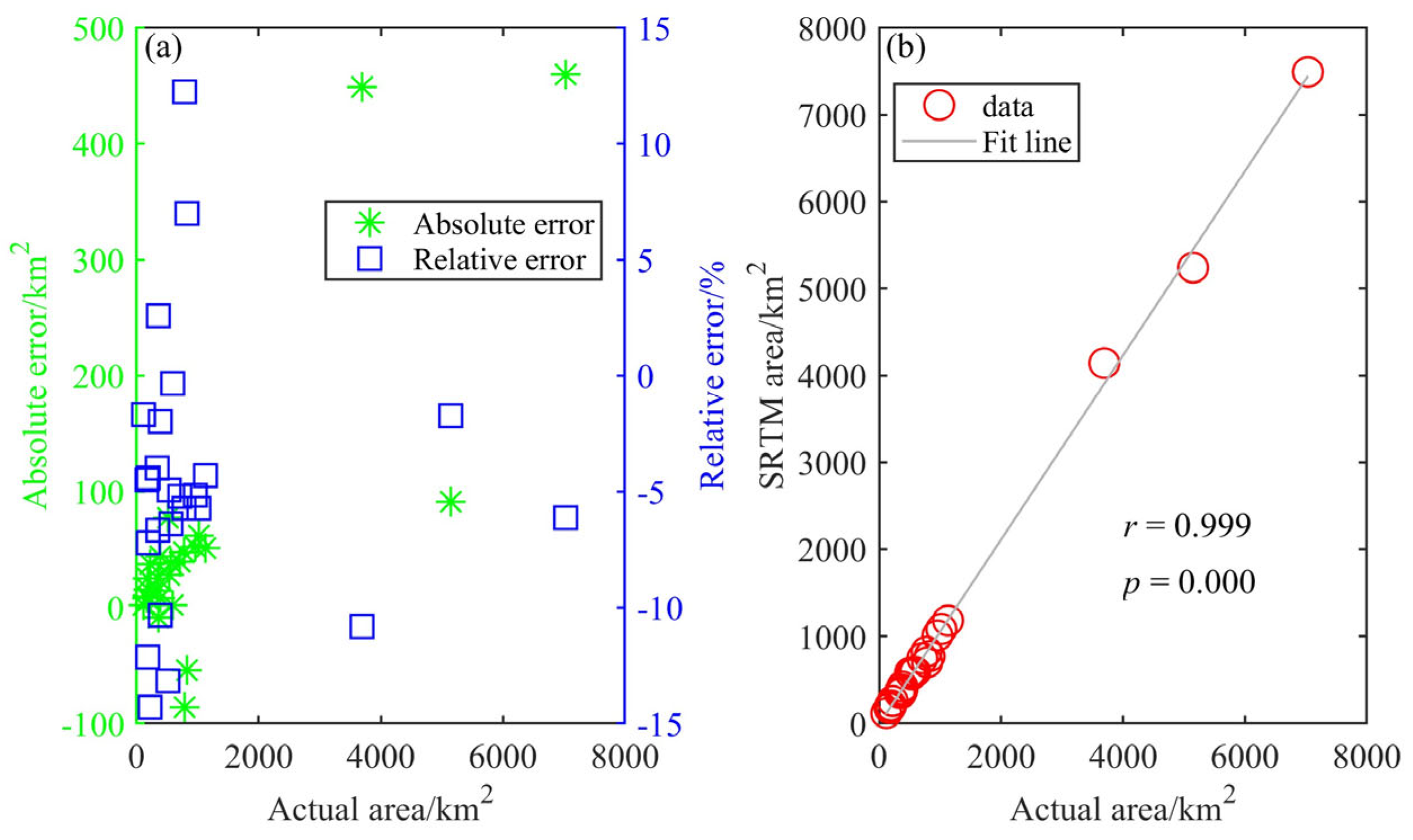
To analyze the extraction accuracy of SRTM watershed characteristic data, this study compared the actual watershed area data obtained from Baidu search, the world’s largest Chinese search engine (https://www.baidu.com/), with the watershed area extracted from SRTM data. The results indicate that the absolute error between the extracted values and the actual values ranges from −86 to 460 m, with an average of 57 m. The relative error between the extracted values and the actual values ranges from −13.16% to 12.25%, with an average of −4.60% (Figure 2a). Pearson correlation analysis shows a strong correlation between the extracted values and the actual values at a confidence level of 0.01 (Figure 2b). Therefore, the watershed area data extracted from SRTM data exhibit high accuracy and can be utilized for subsequent analyses.

3.2. Characteristics of River Parameters

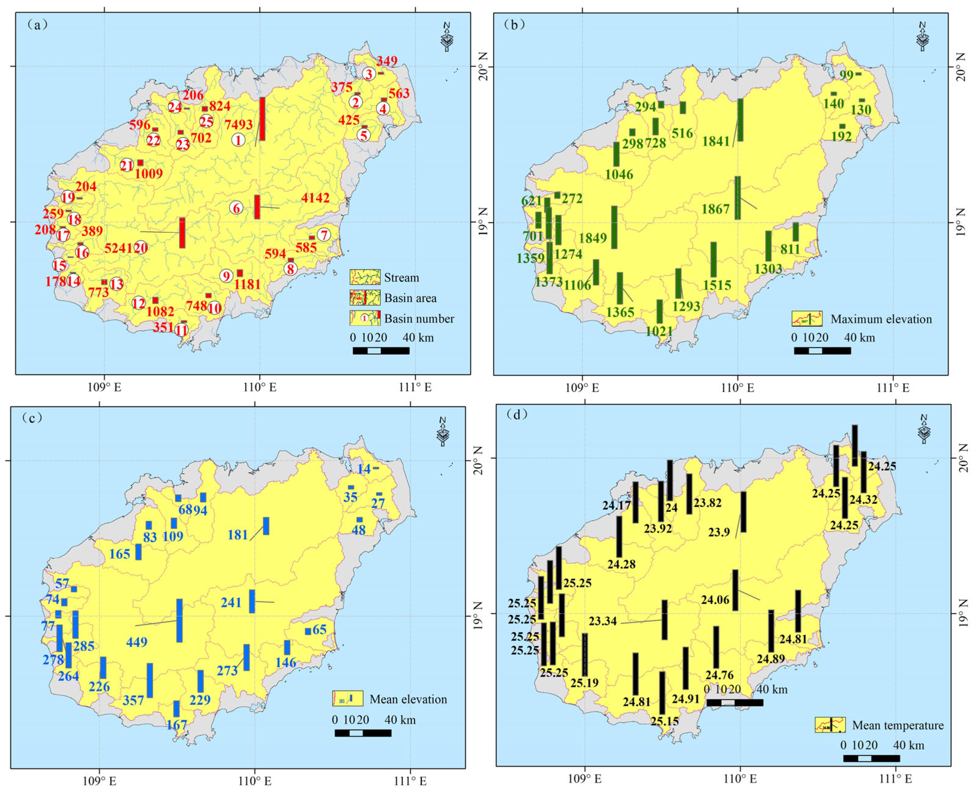
Figure 3 illustrates the spatial characteristics of watershed parameters for the main river basins in the study area. The watershed area ranges from 119 to 7493 km2, with a median of 585 km2 and a mean of 1144 km2. The cumulative area of all major river basins is 28,596 km2, accounting for 84.30% of the total area of the island. The maximum elevation of the watersheds ranges from 99 to 1867 m, with a median of 811 m and a mean of 921 m. Thirteen watersheds, representing 52.00%, have maximum elevations exceeding 1000 m. The average elevation of the watersheds ranges from 14 to 449 m, with a median of 109 m and a mean of 161 m. Similarly, thirteen watersheds, or 52.00%, have average elevations greater than 100 m. The average temperature of the watersheds ranges from 23.82 to 25.25 °C, with a median of 24.34 °C and a mean of 24.62 °C.

3.3. Validation of Qs Calculation Accuracy for Typical Rivers

Table 2 presents the relative errors between the Qs values calculated using different regression equations and the observed values for major rivers in the study area. The Global equation significantly overestimates the Qs for three validation rivers, with an average relative error of 18.73. The range of average relative errors for the same river using different models is between 11.45 and 30.58. Model1 and Model2 exhibit relatively low average relative errors (5.74–5.98), while Model4 is intermediate (14.26), and Model 3 shows a high value (48.95). The use of the Pristine-modified and Disturbed-modified equations significantly improves the calculation accuracy of Qs for the three validation rivers, reducing the average relative errors to 0.72 and 1.64, respectively. When using the Pristine-modified equation, the average relative error ranges for the same river across different models and for the same model across different rivers are −0.04 to 1.97 and 0.41 to 1.32, respectively. In contrast, when using the Disturbed-modified equation, these ranges increase to 0.51 to 3.94 and 1.01 to 2.60, respectively.

3.4. Sediment Flux

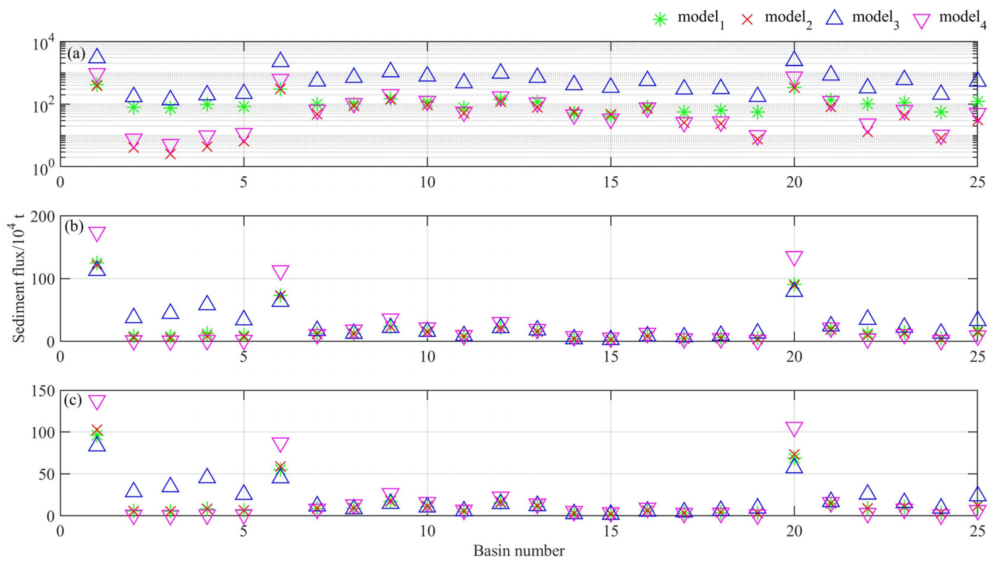
Figure 4 presents the Qs values for the 25 major river basins, calculated using various empirical equations. Regarding the results from the global equation, model3 yields a higher average Qs value for the basins (726.67 × 10⁴ t/a), while model1, model2 and model4 produce lower values (ranging from 83.23 to 147.73 × 10⁴ t/a). Additionally, the cumulative Qs value for model3 (181.67 Mt/a) is an order of magnitude greater than those of the other models (which range from 20.81 to 36.93 Mt/a). In terms of the pristine-modified equation results, model1 and model2 show smaller average Qs values (20.31 to 21.6 × 10⁴ t/a), whereas model3 and model4 exhibit relatively higher values (26.46 to 28.72 × 10⁴ t/a). Furthermore, model1 and model2 have lower cumulative Qs values (5.07 to 7.18 Mt/a), while model3 and model4 present larger values (6.07 to 6.62 Mt/a). For the disturbed-modified equation results, model1 and model2 yield smaller average Qs values (15.78 to 16.56 × 10⁴ t/a), while model3 and model4 show relatively higher values (20.09 to 20.53 × 10⁴ t/a). The cumulative Qs values for model1 and model2 are also lower (3.95 to 4.14 Mt/a), in contrast to the relatively larger values for model3 and model4 (5.02 to 5.13 Mt/a).

4. Discussion

The global empirical equation is a conventional method for calculating Qs; therefore, this study applies the global empirical formula to estimate the Qs of the major rivers flowing into the sea around Hainan Island. However, these results require validation to confirm their accuracy. The most effective validation method involves comparing the calculated results with observed data from hydrological monitoring stations. Unfortunately, the literature indicates that hydrological observation data for rivers in Hainan Island are scarce and primarily concentrated on three major rivers: the Nandu, Changhua, and Wanquan Rivers. Nevertheless, this study compiles the available observational data to serve as validation for the results derived from the Global formula. The findings reveal that when using the global equation to calculate Qs for the validated rivers, the computed results are significantly higher than the observed values. The average relative error for the same river across different models ranges from 11.45 to 30.58, while the average relative error for different rivers using the same model spans from 5.74 to 48.95. Li et al. [19] noted that when applying the global formula to calculate Qs for small rivers discharging into the ocean in southeastern China, the results were 1 to 2 orders of magnitude greater than observed values, which aligns with the findings of this study. Additionally, Milliman et al. [20] pointed out that while the six East Indies islands constitute only about 2% of the land area draining into the global ocean, they discharge approximately 4.2 × 10⁹ t of sediment annually, potentially accounting for 20 to 25% of global sediment export. Thus, the application of global equations may lead to an underestimation result.
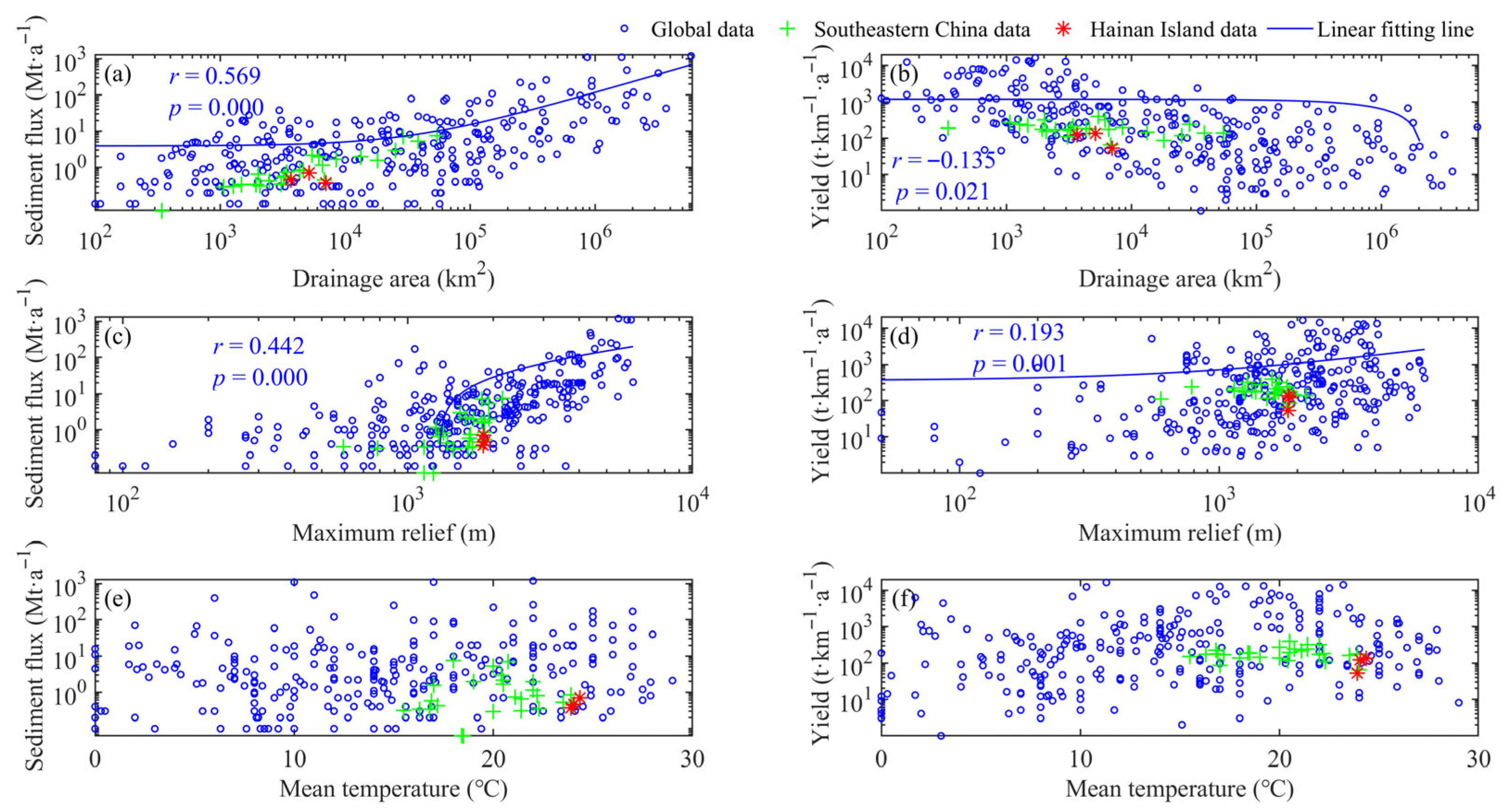
The reason for both the overestimation and underestimation of Qs may mainly cause by the different domain of drainage watershed parameters and regression coefficients between global equations and regional watersheds. For watersheds that establish global equations, their drainage area, maximum relief, mean temperature, sediment flux, and sediment yield are in the range of 102–106 km2, 101–103 m, 0–30 °C, 0.1–1193.4 Mt/a, and 1–16,454 t/(km2·a), respectively [8,16,17,18]. For the southeastern China small watersheds, the responding characteristic values are in the range of 102–104 km2, 102–103 m, 16.3–24 °C, 0.03–7.48 Mt/a, and 51.27–397.95 t/(km2·a), respectively [19]. As for the three representative rivers of Hainan Islands, the responding values are in the range of 3693–7033 km2, 1841–1867 m, 23.90–24.34 °C, 0.37–0.70 Mt/a, and 53.04–135.69 t/(km2·a), respectively [27]. The data points of the southeastern China small watersheds and the representative rivers in Hainan Island located below the linear fitting lines of the global data points (Figure 5). That is, when using the global equations to calculate their sediment flux, their values will show an overestimation result. Based on this, it can be inferred that data points of the six East Indies islands should be drawn on the upper part of the linear fitting lines. As for those watersheds belonging to this kind of river system, the calculation result will be underestimated.
In terms of global model data input points, the flux of sediment entering the ocean shows a moderate correlation with watershed area (r = 0.569) and a weak correlation with maximum elevation (r = 0.442) at a confidence level of 0.01. Conversely, the watershed erosion modulus is essentially uncorrelated with both watershed area and maximum elevation at a confidence level of 0.05 (|r| < 0.2) (Figure 5). This indicates that the Qs is influenced not only by watershed area and maximum elevation but also by other factors within the watershed. Milliman and Meade [13] noted that global model data points exhibit a trend where smaller watersheds have higher erosion moduli, primarily due to the ease with which sediment generated by erosion in small watersheds can be quickly transported to river mouth regions. Furthermore, Milliman et al. [20] highlighted in their study of the six East Indies islands that rivers draining these high-standing islands transport a disproportionately large amount of sediment to the ocean due to their generally small drainage basin areas, high topographic relief, relatively young and erodible rocks, and heavy rainfall.
Research by Syvitski and Milliman [18] indicated that Qs to the ocean is influenced by geological, lithological, topographical, vegetation, temperature, and rainfall factors within the watershed, as well as human intervention activities, which can significantly improve the predictive accuracy of Qs estimates. This study conducts a Sobol sensitivity analysis to identify the relative contribution of each input variable to the Qs. Figure 6 illustrates the distribution of the first-order sensitivity index (S) and total-order sensitivity index (ST) for model2, model3 and model4. The analysis reveals that in model2, variable A exhibits an extremely high sensitivity in the modified equation (approaching 1), while the influence of variable R is relatively minor. In model3, variable R dominates the modified equation, with the effects of variables A and T being comparatively small. In model4, the influences of the three variables (A, R, and T) are relatively balanced, with variable T demonstrating a high sensitivity in the global equation. Comparing the three models, model2 shows extreme variability in sensitivity among the variables, whereas model3 and model4 exhibit a more balanced distribution of variable sensitivity.
This study investigates the changes in sediment concentration and sediment transport in three rivers near hydrological observation stations at the estuaries of Hainan Island, which exhibited significant variability around the year 1980. These changes were primarily influenced by the lagging effects of early human activities and the construction of hydraulic engineering projects during the period from 1956 to 1979 [30]. Specifically, in the Nandu River basin, a series of medium- and small-sized water storage projects were constructed after 1958, controlling an area of over 450 km2, which accounts for 29% of the catchment area of the Longtang hydrological station. Additionally, a dam was completed 1.2 km downstream from the Longtang station in 1970, resulting in a reduction in water flow velocity and a decrease in sediment concentration upstream of the dam. Consequently, the average sediment concentration at the Longtang station from 1980 to 2000 was 44% lower, and sediment transport was 47% lower compared to the period from 1956 to 1979. Similarly, the Wanquan River saw the construction of 15 medium- and small-sized reservoirs after 1958, controlling a total area of 1390 km2, which represents 43% of the catchment area of the Jiaji hydrological station. This led to a 39% reduction in average sediment concentration and a 41% decrease in sediment transport from 1980 to 2000 compared to the 1956 to 1979 period. In the case of the Changhua River, early human activities and hydraulic engineering projects also had a significant impact, resulting in a 19% reduction in average sediment concentration and a 22% decrease in sediment transport at the downstream Baoqiao station from 1980 to 2000 compared to the 1956 to 1979 period.
Li et al. [19] further emphasized that due to the marked differences in Qs before and after large-scale human activities, it is essential to propose distinct correction equations for these two scenarios to enhance the computational accuracy of sediment flux empirical formulas. Specifically, when utilizing global equations, the average relative error between computed values for small rivers in southeastern coastal China and hydrological observation station data ranges from 2.53 to 70.89. In contrast, when applying the pristine-modified and disturbed-modified equations, the average relative errors are significantly reduced to 0.07–0.1 and 0.18–0.24, respectively. The findings of this study also indicate that when employing global formulas, the relative error of computed results is substantial, ranging from 11.45 to 30.58. However, the use of modified equations leads to a marked improvement in relative error, with average relative errors reduced to −0.04 to 1.97 and 0.51 to 3.94 for the pristine-modified and disturbed-modified equations, respectively. Therefore, when calculating sediment flux for small rivers, it is crucial to not only adjust global empirical formulas but also to differentiate between the scenarios of before and after large-scale human activities.
The results of the Monte Carlo simulation uncertainty analysis indicate significant differences among the various models (Table 3). Model3’s global equation exhibits the highest volatility, with a mean of 13.22 and a standard deviation of 6.06, resulting in a 95% confidence interval spanning 21.7, which suggests a high level of uncertainty in this model’s calculations. In contrast, the disturbed-modified equation demonstrates the greatest stability among all models; for instance, Model4’s disturbed-modified equation has a standard deviation of only 0.31 and a confidence interval width of 1.11, indicating greater reliability. Overall, the results from the global equations tend to be higher than those from the modified equations, with a mean difference of 4.8 times between Model1 and Model3. The means of the modified equations (Pristine/Disturbed-modified) are consistently within the range of 0.42 to 1.19, with standard deviations below 1.04. Notably, Model4’s disturbed-modified equation has a lower limit of 0.03, demonstrating superior resistance to disturbances. It is recommended that the disturbed-modified equation be prioritized in high-risk scenarios, and if the global equation must be utilized, the applicability of Model4 should be thoroughly validated.
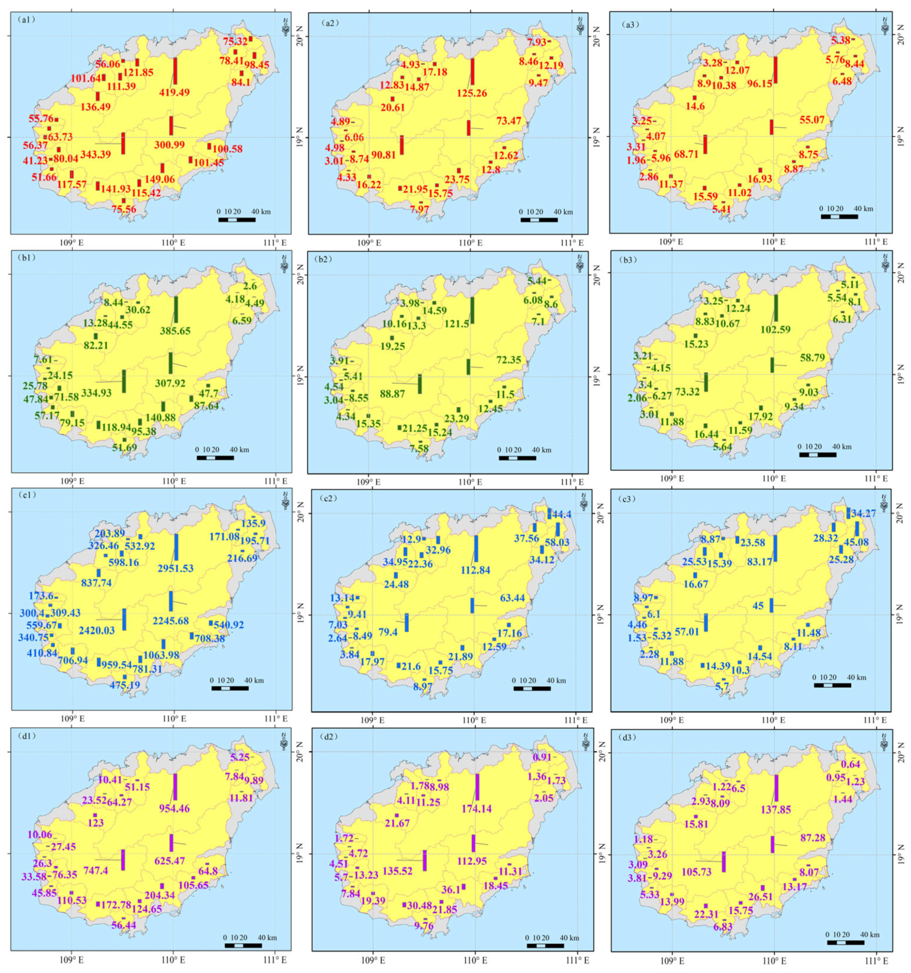
Figure 7 and Table 4 present the spatial distribution and statistical characteristics of Qs from the major rivers of Hainan Island, as calculated by different methods. Overall, the results reveal a consistent trend where larger watershed areas and greater maximum elevations correspond to higher values of Qs. For the global empirical formula, the cumulative Qs values for all watersheds calculated by different models range from 20.81 to 181.67 Mt/a. This result may significantly exceed actual values, primarily due to the high relative error (11.45–30.58) observed in the calculations for three validation rivers when using the global formula. In the case of the pristine-modified and disturbed-modified equations, the cumulative Qs results from different models are relatively close, with ranges of 5.08–7.18 Mt/a and 3.95–5.13 Mt/a, respectively. Although differences exist among models related to the weighting of controlling factors, the inter-model relationships also indicate mutual validation, suggesting that the computational results are highly reliable. Therefore, this study proposes that the average of the results from different models can be used to obtain the target watershed’s Qs. Based on this, the Qs for the major rivers of Hainan Island under the scenarios of before and after large-scale human activities are estimated to be 6.07 Mt/a and 4.56 Mt/a, respectively.
It is important to note that the method used in this study to calculate Qs pertains solely to the suspended sediment flux entering the sea from the watersheds of 25 major rivers in Hainan Island. It does not account for other rivers or the material flux generated by the erosion of bedrock coastlines and varying catchment background. Future research should continue to focus on the following areas: (1) collecting additional data from hydrological observation stations to enhance the calibration accuracy of global empirical formulas; (2) developing and calculating methods and fluxes for estimating Qs resulting from erosion of bedrock coastlines; and (3) conducing comparative studies on a wider range of island systems with varying climate, geological, and anthropogenic influences.

5. Conclusions

(1) The area values of watersheds extracted from SRTM data exhibit a high correlation with actual values at a confidence level of 0.01, with an average relative error of −4.60%.
(2) The global equation significantly overestimates Qs for the validation rivers, with an average relative error of 18.73. In contrast, employing the pristine-modified and disturbed-modified equations effectively improves the calculation accuracy of Qs for the validation rivers, reducing the average relative errors to 0.72 and 1.64, respectively.
(3) By averaging the results from different models, this study estimates that the Qs for the major rivers in Hainan Island was 6.07 Mt/a before large-scale human activities and 4.56 Mt/a after.

Author Contributions

G.L.: Formal analysis; Conceptualization; Funding acquisition; Writing—original draft. L.D.: Formal analysis; Visualization. L.H.: Investigation; Data curation. C.T.: Conceptualization; Formal analysis; Writing—review & editing. All authors have read and agreed to the published version of the manuscript.

Funding

Opening Foundation of Hainan Key Laboratory of Marine Geological Resources and Environment (No. HNHYDZZYHJKF015); Project for Enhancing the Practical and Innovative Abilities of Postgraduates at Guangdong Ocean University (No. 100204/080504112505).

Data Availability Statement

The raw data supporting the conclusions of this article will be made available by the authors on request.

Acknowledgments

Special thanks to the editor and anonymous reviewers who have helped with the improvement of the paper. It should be noted that the first and second affiliations contributed equally as co-first affiliations.

Conflicts of Interest

This statement is to declare that authored by Li et al. have no financial and personal relationships with other people or organizations that can inappropriately influence our work, there is no professional or other personal interest of any nature or kind in any product, service and/or company that could be construed as influencing the position presented in, or the review of, the manuscript.

References

  1. Li, G.C.; Gao, S.; Wang, Y.P.; Li, C.Y. Sediment flux from the Zhoushan Archipelago, eastern China. J. Geogr. Sci. 2018, 28, 387–399. [Google Scholar] [CrossRef]
  2. Jia, J.J.; Gao, J.H.; Cai, T.L.; Li, Y.; Yang, Y.; Wang, Y.P.; Xia, X.M.; Li, J.; Wang, A.J.; Gao, S. Sediment accumulation and retention of the Changjiang (Yangtze River) subaqueous delta and its distal muds over the last century. Mar. Geol. 2018, 401, 2–16. [Google Scholar] [CrossRef]
  3. Bianchi, T.S.; Allison, M.A. Large-river delta-front estuaries as natural “recorders” of global environmental change. Proc. Natl. Acad. Sci. USA 2009, 106, 8085–8092. [Google Scholar] [CrossRef]
  4. Gao, S.; Collins, M.B. Holocene sedimentary systems on continental shelves. Mar. Geol. 2014, 352, 268–294. [Google Scholar] [CrossRef]
  5. Day, J.W.; Agboola, J.; Chen, Z.Y.; D’Elia, C.; Forbes, D.L.; Giosan, L.; Kemp, P.; Kuenzer, C.; Lane, R.; Ramachandran, R.; et al. Approaches to defining deltaic sustainability in the 21st century. Estuar. Coast. Shelf Sci. 2016, 183, 275–291. [Google Scholar] [CrossRef]
  6. Milliman, J.D.; Farnsworth, K.L. River Discharge to the Coastal Ocean: A Global Synthesis; Cambridge University Press: Cambridge, UK, 2013; pp. 1–20. [Google Scholar]
  7. Guo, L.C.; Su, N.; Townend, I.; Wang, Z.B.; Zhu, C.Y.; Wang, X.Y.; Zhang, Y.N.; He, Q. From the headwater to the delta: A synthesis of the basin-scale sediment load regime in the Changjiang River. Earth-Sci. Rev. 2019, 197, 102900. [Google Scholar] [CrossRef]
  8. Milliman, J.D.; Syvitski, J.P.M. Geomorphic/tectonic control of sediment discharge to the ocean: The importance of small mountainous rivers. J. Geol. 1992, 100, 525–544. [Google Scholar] [CrossRef]
  9. Ahnert, F. Functional relationships between denudation, relief, and uplift in large, mid-latitude drainage basins. Am. J. Sci. 1970, 268, 243–263. [Google Scholar] [CrossRef]
  10. McLennan, S.M. Weathering and global denudation. J. Geol. 1993, 101, 295–303. [Google Scholar] [CrossRef]
  11. Wang, Y.P.; Pan, S.M.; Wang, H.V.; Gao, J.H.; Yang, Y.; Wang, A.J.; Li, Z.H.; Wu, Z. Measurements and analysis of water discharges and suspended sediment fluxes in Chinajiang Estuary. Acta Geogr. Sin. 2006, 61, 35–46. (In Chinese) [Google Scholar] [CrossRef]
  12. Holeman, J.N. The sediment yield of major rivers of the world. Water Resour. Res. 1968, 4, 737–747. [Google Scholar] [CrossRef]
  13. Milliman, J.D.; Meade, R.H. World-wide delivery of river sediment to the oceans. J. Geol. 1983, 91, 1–21. [Google Scholar] [CrossRef]
  14. Li, G.C.; Zhou, L.; Qi, Y.L.; Gao, S. Threshold sediment flux for the formation of river deltas in Hainan Island, southern China. J. Geogr. Sci. 2019, 29, 146–160. [Google Scholar] [CrossRef]
  15. Molliex, S.; Kettner, A.J.; Laurent, D.; Droz, L.; Marsset, T.; Laraque, A.; Rabineau, M.; N’Kaya, G.D. Simulating sediment supply from the Congo watershed over the last 155 ka. Quat. Sci. Rev. 2019, 203, 38–55. [Google Scholar] [CrossRef]
  16. Mulder, T.; Syvitski, J.P.M. Climatic and morphologic relationships of rivers: Implications of sea-level fluctuations on river loads. J. Geol. 1996, 104, 509–523. [Google Scholar] [CrossRef]
  17. Syvitski, J.P.M.; Peckham, S.D.; Hilberman, R.; Mulder, T. Predicting the terrestrial flux of sediment to the global ocean: A planetary perspective. Sediment. Geol. 2003, 162, 5–24. [Google Scholar] [CrossRef]
  18. Syvitski, J.P.M.; Milliman, J.D. Geology, geography, and humans battle for dominance over the delivery of fluvial sediment to the coastal ocean. J. Geol. 2007, 115, 509246. [Google Scholar] [CrossRef]
  19. Li, G.C.; Xia, Q.; Fu, D.Y.; Zeng, C.H.; Li, Z.Q.; Gao, S. Calculating the sediment flux of the small coastal watersheds: A modification of global equations. Acta Oceanol. Sin. 2021, 40, 147–154. [Google Scholar] [CrossRef]
  20. Milliman, J.D.; Farnsworth, K.L.; Albertin, C.S. Flux and fate of fluvial sediments leaving large islands in the East Indies. J. Sea Res. 1999, 41, 97–107. [Google Scholar] [CrossRef]
  21. Dadson, S.J.; Hovius, N.; Chen, H.; Dade, W.B.; Hsieh, M.L.; Willett, S.D.; Hu, J.C.; Horng, M.J.; Chen, M.C.; Stark, C.P.; et al. Links between erosion, runoff variability and seismicity in the Taiwan orogen. Nature 2003, 426, 648–651. [Google Scholar] [CrossRef]
  22. Wang, Y.; Zhou, L.F. The volcanic coast in the area of northwest Hainan Island. Acta Geogr. Sin. 1990, 50, 321–330. (In Chinese) [Google Scholar] [CrossRef]
  23. Wang, Y.; Peter, M.I.; Zhu, D.K.; Zhang, Y.Z.; Tang, W.W. Coastal plain evolution in southern Hainan Island, China. Chin. Sci. Bull. 2001, 46, 90–96. [Google Scholar] [CrossRef]
  24. Wu, S.A.; Xing, C.Y.; Zhu, J.J. Analysis of Climate characteristics in Hainan Island. J. Trop. Biol. 2022, 13, 315–323. (In Chinese) [Google Scholar] [CrossRef]
  25. Yao, L.P.; Wang, X.; Zhang, J.H.; Yao, F.M. Analysis of spatio-temporal variation and driving forces of leaf area index in Hainan Island over the last 20 years based on MODIS data. Chin. J. Eco-Agric. 2024, 32, 1719–1930. (In Chinese) [Google Scholar] [CrossRef]
  26. Wang, W.J.; Jin, Z.M.; Bao, Q.S. Characteristic of natural conditions and the construction of ports in the coastal areas of Hainan Island. Trop. Geogr. 1983, 3, 8–13. (In Chinese) [Google Scholar]
  27. Yang, Z.H.; Jia, J.J.; Wang, X.K.; Gao, J.H. Characteristics and variations of water and sediment fluxes into the sea of the top three rivers of Hainan in recent 50 years. Mar. Sci. Bull. 2013, 32, 92–99. (In Chinese) [Google Scholar] [CrossRef]
  28. Nienhuis, J.H.; Ashton, A.D.; Giosan, L. What makes a delta wave-dominated? Geology 2015, 43, 511–514. [Google Scholar] [CrossRef]
  29. Gao, S.; Zhou, L.; Li, G.C.; Wang, D.D.; Yang, Y.; Dai, C.; Han, Z.C.; Wang, H.; Tu, J.Y.; Yang, B.M. Processes and sedimentary records for Holocene coastal Environmental changes, Hainan Island: An overview. Quat. Sci. 2016, 36, 1–17. (In Chinese) [Google Scholar] [CrossRef]
  30. Li, L.B. Analysis of the trend of sediment changes in major rivers in Hainan Island. In Proceedings of the 3rd Youth Science and Technology Forum of the Chinese Water Conservancy Society, Chengdu, China, 11–13 October 2007; pp. 280–284. [Google Scholar]
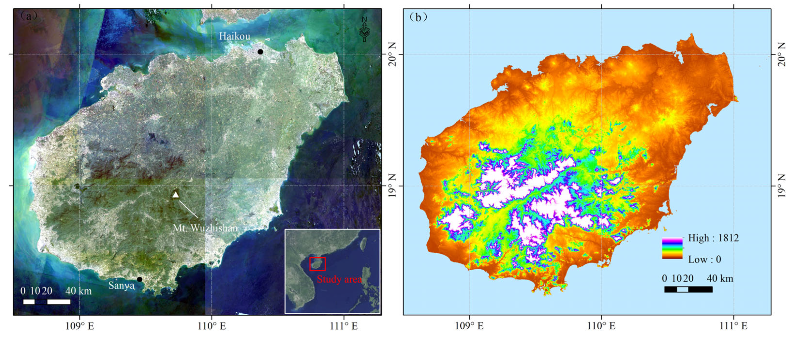
Figure 1. Remote sensing image (a) and SRTM (b) of the study area.
Jmse 13 02039 g001
Figure 2. Absolute error (a) and relative error (b) of watershed area data extracted from SRTM data.
Jmse 13 02039 g002
Figure 3. Distribution of (a) watershed area, (b) maximum elevation, (c) average elevation, and (d) average temperature for major river basins in Hainan Island.
Jmse 13 02039 g003
Figure 4. Qs of the 25 main river basins in Hainan Island calculated by: the global equations (a); the pristine-modified equations (b); the disturbed-modified equations (c).
Jmse 13 02039 g004
Figure 5. Relationship between annual Qs (a,c,e) or sediment yield (b,d,f) and watersheds characteristics for the database of the Global equation, the small coastal watersheds in southeastern China and the three representative rivers in Hainan Islands.
Jmse 13 02039 g005
Figure 6. First-order sensitivity index (S) and Todal-order sensitivity index (ST) of the different Qs calculation models based on Sobol sensitivity analysis method. (a) Global equation vs. Model2; (b) Global equation vs Model3; (c) Global equation vs. Model4; (d) Pristine-modified equation vs. Model2; (e) Pristine-modified equation vs. Model3; (f) Pristine-modified equation vs. Model4; (g) Disturbed-modified equation vs. Model2; (h) Disturbed-modified equation vs. Model3; (i) Disturbed-modified equation vs. Model4.
Jmse 13 02039 g006
Figure 7. Distribution of the Qs calculated by different regression equations. Global equation: Model1 (a1), Model2 (b1), Model3 (c1) and Model4 (d1); Pristine-modified equation: Model1 (a2), Model2 (b2), Model3 (c2) and Model4 (d2); Disturbed-modified equation: Model1 (a3), Model2 (b3), Model3 (c3) and Model4 (d3).
Jmse 13 02039 g007
Table 1. The values of regression coefficients of global equations and modified equations.
Regression CoefficientGlobal EquationPristine-Modified EquationDisturbed-Modified Equation
a65.00102.4895.67
b0.560.900.94
c0.410.880.94
d1.280.140.04
f−3.68−2.28−2.26
g0.450.951.01
h0.57−0.68−0.76
i−0.09−0.02−0.03
j0.080.040.05
k0.800.970.95
l0.310.821.08
m0.50−0.03−0.22
Table 2. Relative errors of the Qs calculated by the different regression equations.
EquationRiverObservation
(104 t/a)
Model1Model2Model3Model4Model Averaging
Result (104 t/a)REResult (104 t/a)REResult (104 t/a)REResult (104 t/a)REResult (104 t/a)RE
Global
equation
Nandu37.30419.4910.25385.659.342951.5378.13954.4624.591177.7830.58
Changhua69.88300.993.31307.923.412245.6831.14625.477.95870.0111.45
Wanquan45.33343.396.58334.936.392420.0352.39747.4015.49961.4420.21
Basin averaging50.84354.625.98342.835.742539.0848.95775.7814.261003.0818.73
Pristine-modified equationNandu44.99125.261.78121.651.70112.841.51174.142.87133.481.97
Changhua83.8473.47−0.1272.35−0.1463.44−0.24112.950.3580.55−0.04
Wanquan52.9790.810.7188.870.6879.400.50135.521.5698.650.86
Basin averaging60.6096.510.5994.290.5685.230.41140.871.32104.230.72
Disturbed-modified equationNandu21.2496.153.53102.593.8383.172.92137.855.49104.943.94
Changhua40.7055.070.3558.790.4445.000.1187.281.1461.540.51
Wanquan30.0468.711.2973.321.4457.010.90105.732.5276.191.54
Basin averaging30.6673.311.3978.231.5561.731.01110.292.6080.891.64
Table 3. Uncertainty quantification results of the different Qs calculation models based on Monte Carlo simulation.
Calculation ModelMean QsStandard Deviation95% Confidence Interval
Model1Global equation2.770.97[0.81, 4.14]
Pristine-modified equation0.690.34[0.09, 1.23]
Disturbed-modified equation0.510.27[0.06, 0.94]
Model2Global equation1.300.91[0.09, 3.26]
Pristine-modified equation0.590.30[0.08, 1.12]
Disturbed-modified equation0.520.28[0.06, 0.98]
Model3Global equation13.226.06[3.34, 25.04]
Pristine-modified equation1.191.03[0.10, 4.16]
Disturbed-modified equation0.960.96[0.06, 3.85]
Model4Global equation0.960.62[0.11, 2.29]
Pristine-modified equation0.550.40[0.05, 1.45]
Disturbed-modified equation0.420.31[0.03, 1.14]
Table 4. Statistical characteristic values of Qs calculated by different regression equations.
Calculation EquationVariablesQs (×104 t/a)
Model1Model2Model3Model4Model Averaging
Global EquationMin41.232.60135.905.2554.77
Max419.49385.652951.53954.461177.78
Mean123.1283.23726.67147.73270.19
SD91.70103.25722.00242.20288.63
Total3077.942080.7218,166.743693.286754.67
Pristine-modified equationMin3.013.042.640.913.60
Max125.26121.65112.84174.14133.48
Mean21.6420.3128.7226.4624.28
SD29.1628.7525.6044.1031.06
Total541.07507.82717.92661.51607.08
Disturbed-modified equationMin1.962.061.530.642.34
Max96.15102.5983.17137.85104.94
Mean15.7816.5620.5320.0918.24
Std.22.4124.0119.1634.7324.37
Total394.59413.96513.24502.29456.02
Disclaimer/Publisher’s Note: The statements, opinions and data contained in all publications are solely those of the individual author(s) and contributor(s) and not of MDPI and/or the editor(s). MDPI and/or the editor(s) disclaim responsibility for any injury to people or property resulting from any ideas, methods, instructions or products referred to in the content.