Abstract
The assessment for the resistance of a new ship under design can be performed through the Experimental Fluid Dynamics (EFD) or the Computational Fluid Dynamics (CFD) approach; both have their own Uncertainty Assessment (UA). In CFD field, the Verification and Validation (V&V) procedures take into account the approximations for numerical issues and the assumptions adopted to describe the physical phenomena to assess UA. Different theoretical approaches have become available over time; nevertheless, a single comprehensive solution to achieve the UA remains still unknown because as the theoretical methodology varies, the outcome changes. In current work, four different literature approaches will be augmented to perform a V&V analysis for two kinds of model hulls, tested at different speeds and compared with the experimental data. The investigations performed among results lead to the division of all the approaches into the three and four solutions families and to define a robust procedure to identify a reasonable value for the numerical uncertainty assessment. Regarding the robustness and the UA of the approaches, the first family proved successful in only 55% of cases with a UA mean value below 2.01%, while the second one always provides a quantification but with a mean value of 6.65%.
1. Introduction
During the design phase of a new ship, the preliminary evaluation for its total resistance is affected by an uncertainty result, even though the definition of the problem is dated back to the beginning of the second half of the 19th century, since the power propulsion plans transitioned from sails to internal or external combustion engine.
William Froude, a pioneer in the attempt to evaluate the total resistance for a ship, considered the total resistance as a sum of several components [1] and in 1868 he performed an experimental procedure to scale from the results obtained for a model-scale ship towed inside a towing tank to the full-scale one. From, that time, which can be recognized as the beginning of the Experimental Fluid Dynamic (EFD), further implementations about the procedure were performed among the scientific community [2], leading to procedures constantly updated and freely accessible through the “Recommended Procedures and Guidelines” repository [3], held by the International Towing Tank Conference (ITTC). Concurrently with the developments of EFD procedure, considering the improvements for the solution of the Navier–Stokes equations registered by the early 1950’s [4], the scientific community increasingly relies on Computational Fluid Dynamics (CFD) to perform models and to predict fluid flow behaviors, as an alternative way to the EFD results. Considering the potentiality offered by CFD, the scientific community organized several international workshops to assess the effectiveness of the methods; among them, the first of these was held in Gothenburg in 1980, with many others following over the years [5,6].
Regarding the growth of available methodologies offered by EFD and CFD to predict ship resistance, their results are still affected by uncertainty. Considering the CFD, the UA can be performed through a two-step procedure: the first, verification, defines the numerical uncertainty; and the second, validation, assesses the uncertainty for the modelling assumptions.
In line with the research performed by Islam and Guedes Soares [7] to identify the uncertainty prediction through two different theoretical approaches, the current research uses other literature available approaches and tries to identify a reasonable value for the numerical Uncertainty Assessment (UA). Accordingly, after a brief description about the available theoretical approaches proposed by Celick [8], Stern et al. [9,10] and Eça and Hoekstra [11] will be given along with the numerical set-up applied to the CFD calculations. Later on, two different hulls, tested at different speed and conditions (a total of 72 simulations have been performed in the OpenFOAM environment) are going to be used to get the UA for the resistance prediction with the proposed methodologies.
Current research primarily focuses on data analysis to identify the strengths and weaknesses of the proposed methodologies, aiming to address the existing gap in knowledge regarding numerical uncertainty assessment. Additionally, it seeks to establish best practices for defining a robust procedure to evaluate numerical uncertainty.
2. Verification, Validation and Uncertainty Assessment (VVUA)
During the tests, the data are handled using international standard methodologies for uncertainty evaluation, while carefully accounting for experimental errors in the obtained results; indeed, “all the relevant parameters are affected by uncertainty and its assessment is necessary to provide the required confidence intervals of all relevant variables used for validation” [12]. While, following the development of CFD predictions, in the last decades several types of approaches can be listed in the field of Verification, Validation and Uncertainty Assessment (VVUA) [13].
All the VVUA procedures follow a procedure based on three main sections and can be schematically represented through the Figure 1.
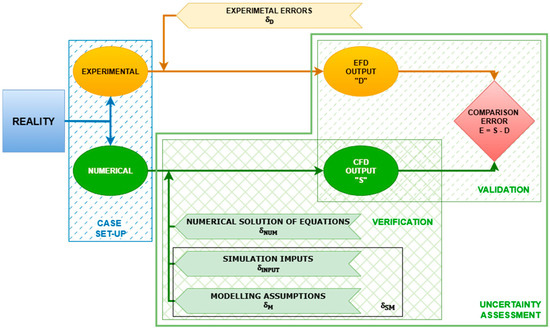
Figure 1.
Schematic representation of the flow chart describing the uncertainty assessment applied to a CFD calculation, which provides an evaluation of the resistance for a model-scale hull tested in a towing tank (EFD).
2.1. Uncertainty Assessment
The uncertainty assessment (UA) intends to evaluate, by applying a mathematical and procedural algorithm, the uncertainties and the errors deriving from all kinds of sources, both for numerical calculations and for experimental tests.
As reported in Sadrehaghighi’s work [14] where the definitions of the AIAA Guidelines are implemented [15], uncertainty, , can be seen as “A potential deficiency in any phase or activity of the modeling process that is due to the lack of knowledge”, rather error, , as “A recognizable deficiency in any phase or activity of modeling and simulation that is not due to lack of knowledge”.
If the uncertainty is an estimation of the error between reality and the data with a level of confidence of 95%, a CFD calculation incorporates error and uncertainties deriving from the modeling of the physical phenomena and the numerical resolution of the equations. In particular, in CFD applications, the first type of error, , comes from the assumptions performed to describe the physical problem (geometrical approximations, boundary conditions, mathematical equations, fluid properties, etc.), the second one, , differently, is connected with the numerical solution of the mathematical equations (such as discretization, computer round-of, etc.). Consequently, the simulation error, , can be mathematically expressed by Equation (1):
where represents the true value and the simulation result, while represents the modelling simulation error, seen as the difference between the model value and the true one, and the numerical simulation error, seen as the difference between the model value and the simulation result. The simulation uncertainty, , can consequently be calculated as reported in Equation (2):
where stands for modelling uncertainty and for numerical uncertainty. Regarding , it is possible, under conditions, to define it through Equation (3):
where is the error estimate and the estimate of sign and magnitude of . It is possible to achieve the correct simulation value, Sc, and its error and uncertainty, respectively and , by the Equations (4)–(6).
where is the uncertainty estimate for . The scientific technical debate remains open regarding the error’s evaluation, ; two approaches can be considered [9]: the deterministic one for the “corrected” approach, as proposed by Coleman [16] and the stochastic one for the “uncorrected” approach, as proposed by Oberkampf and Trucano [17].
Both following paragraphs, considering the naval architecture fields from which the results coming from the EFD tests are compared with the CFD simulations one, to account for the uncertainty assessment (UA) through the evaluation of both numerical uncertainties, , and the modelling assumptions, , respectively define the Verification and the Validation assessments.
2.2. Verification
The verification procedure deals with the mathematical solution of the chosen equation to describe phenomena. The evaluation of the simulation numerical Uncertainty, , is the target of this procedure and, when it’s possible, to assess the sign and the magnitude of the simulation numerical error, . Two kinds of investigations can be performed: the code verification and the solution verification; current work deals with the second one, considering the code as already verified by code developer. It is possible to split and consequently into subcomponents as reported in (7) and (8):
where the subscripts denote the contributions coming from the grid size ( and ), the iteration number ( and ), the step ( and ) and other parameters ( and ), respectively. Moreover, the corrected simulation, , and its numerical uncertainty , can be performed through (9)–(12):
By looking at (11), can be seen as a correct value, , more than a correction due to a numerical error.
All the methodologies available nowadays are based on the Richardson Extrapolation (RE) [18] to perform the Verification assessment because of its ability to increase the numerical precision based on the power series expansion for the results obtained for discretized points. Moreover, addressing the estimation for the numerical discretization error, , and its uncertainty, , different kinds of approaches are available, and both unstructured and structured mesh can be listed and investigated in what follows.
Convergence study. In convergence study, the iterative convergence methodology is applied to evaluate numerical uncertainty; in this kind of approach one parameter changes while all the others remain unchanged and multiple solutions (at least three) are required to assess if the convergence has been achieved. Focused attention must be carried out to the variation of the input parameter, defined as refinement ratio parameter . In fact, the parameter should be carefully chosen among two antithetical conditions: bigger enough to make the input parameter unsensible to the numerical noise and smaller enough to be computationally affordable. Nowadays, scientific debate on the value for remains still open; the suggested theorical value for a 3D simulation is , but for industrial studies the computational effort required is higher than the one sustainable and the suggested one consists of or 1.3. As reported in (7, 8), the total numerical uncertainty and its error can be considered as the sum of different kinds of contributions. Following Stern results for a steady-state simulation [19], only contributions due to iteration number and grid size are considered; and going into further detail, grid uncertainty is the predominant, and therefore iteration contribution can be neglected, as reported by Huang et al. [20] and Lakatoš et al. [21], reaching the Equations (13) and (14):
The numerical uncertainty is directly linked to the grid inside the numerical simulation volume. Considering that the mesh can be either structured or unstructured, where the simulation works with a structured mesh it is possible to get a mathematical hierarchical relationship based on the parameter among them, whereas it is not feasible in the other case. This means that for the structured 3D meshes, the grid ratio parameter can be exactly the one suggested ad constant by changing the size of the meshes (, being N the number of cells inside the domain, with ); while, for unstructured meshes, it is not perfectly feasible (, noted that and ). With the respect of the mesh size, the convergence study can be performed with a minimum number of three solutions , being the solution for the fine mesh with cells, for the generally reference one with cells and for the coarse one with cells. The ratio of solution change, , can be defined with (15) by comparing the three solutions:
Looking at its value, it is possible to achieve 4 conditions:
- Monotonic convergence if ;
- Oscillatory convergence if ;
- Divergence if ;
- Oscillatory divergence if and .
where monotonic convergence occurs, the generalized Richardson Extrapolation is used to assess and . Whereas, instead, oscillatory convergence is reached, it is only possible to assess the without sign by bounding it among the values of the upper () and lower () solutions, as reported in (16). In case of divergence, instead, further investigations have to be carried out because nothing can be settled in this condition.
The limit of three solutions methods relates to the relative positioning between solutions and discretization. The two principal cases where the method shows limits are: the case of oscillatory convergence because it can hide a real monotonic convergence or divergence, as reported by Coleman et al. [22], and the case where the difference among solutions is close to zero () with a hill conditioned ratio like in presence of an inflection point. To address these issues further, other methods are available; among them the one based on Least Squares Root (LRS) as proposed by Eça and Hoekstra [11]. It will be analyzed in paragraph 4 (Verification and Validation) due to its ability to account for scatter in numerical solutions.
In the field of steady CFD computations to assess numerical uncertainty, the most used methodology works with discretized data obtained by systematical grid refinement. Each one differs in the number of solutions to be considered and in how to assess approximate mean behavior among them; rather, all of them estimate the error with a power series expansion based on cell size as proposed in RE and differ again in how to account for the approximations imposed by RE theory. Before going into the details of each methodology and the results obtained, a first key difference between them can be observed: each procedure requires multiple solutions to function properly, and each solution demands computational resources. Moreover, the computational effort increases more than a factor one with the increase of the refinement. Therefore, transitioning from a methodology that requires a minimum of three solutions to one that requires at least four entails a significantly greater computational cost, which may not be negligible.
Celik et al. They [8] proposed a practical guideline based on RE introducing the Grid Convergence Index (GCI) divided into 5 steps. Steps 1 and 2 deal with the discretization operations (the suggested and not mandatory value for the refinement ratio parameter, is such that , constant by varying). In step 3 and 4, the apparent order of accuracy, p, and the extrapolated value of the solution, , are evaluated considering an infinite number of cells. Using a fixed-point iteration, it’s possible to solve it easily (17)–(19) obtaining .
With (20) it is possible to calculate the extrapolated value .
The last step, instead, deals with the estimates of approximate relative error (21), the interpolated relative error (22) and the fine-grid convergence index (23) which represent an index useful to assess the obtained accuracy.
Generalized Richardson Extrapolation, Stern et al. When the convergence analysis achieves a monotonic behavior, generalized RE can be used to evaluate , and . As reported by Stern et al. [9], to account for the high orders terms in RE power series expansion, analytical benchmark can be used to fit a correction; among the corrections, two kinds of approach can be followed: correction factor, as reported by Stern et al. [9] and/or factor of safety as proposed by Roache [23]. As reported in (12), and considering the convergence study based on the grid refinements, the accuracy of the error can be evaluated by considering the order of the power series expansion. Where 3 solutions are available and where a constant grid refinement parameter is achieved, only the leading term of the expansion, , and its order of accuracy, , can be estimated as reported in (24) and (25)
Further improvements can be implemented in (25) to account for solutions in more than 3 cases, but the range of applicability criterion for the solutions is more restrictive since the mandatory condition of monotonic convergence and the closeness to the asymptotic range; moreover, if the grid refinement factor is not constant, Equation (26) has to be applied:
In Equation (26), if , returns the same result of (25); while, if , becomes a transcendent implicit equation, which resolution can be achieved by an iterative procedure. Herein, to account for the effects of high order terms in power series expansion on estimating errors and uncertainties, different methodologies will be presented consistently applied to the generalized RE. The factor of safety approach, proposed by Roache [23], can be used to define by multiply the with the factor itself to bound the error, as exposed in (27).
where is the factor of safety. Different kinds of formulations are available for the definition of . With reference to , Roache [23] recommends a value of 1.25 and a value of 3 when only 2 grids are available. Based on this approach, even if not proposed by Roache, it is possible to assess the value of following Equation (28):
Another approach to evaluate was proposed by Xing et al. in 2010 [10]. In this approach the value of was determined by Equation (29), which takes into account both the value of a distance metric, (defined as ), and the findings of a statistical analysis based on a large number of numerical or analytical benchmarks to fit the values for the coefficients.
This last approach has been also reported into the last ITTC procedure for Uncertainty Analysis in CFD Verification and Validation, Methodology and Procedures [13]. Using a correction factor approach to account for the influence of higher-order terms, a multiplicative factor , is applied to , as reported in Equation (30).
The suitable value for can be evaluated thought two procedures: the first one, roughly considers the effects of high order term (31); the second one, in a more rigorous manner, utilizes a two-term estimation (32).
Equation (31) coincides with (32) when the asymptotic range has been achieved. When is close to one, Equations (24) and (30) coincide and the asymptotic range has been achieved and having confidence and can be evaluated through (33).
where, when 1, because of the limit of the asymptotic range. Whereas, outside the asymptotic range, and the influence of the high-order terms of the expansion cannot be neglected, otherwise an overestimation or an underestimation () can occur. In this last case, can be estimate through (34), but not and .
Eça and Hoekstra. As reported in [11], when complex geometries and equations are involved in the case under study, it becomes essential to ensure consistency with the results of the grid refinement study, the following assumptions can be hard to be numerically achieved: asymptotic range and data without scatter. The presence of scatter results is common in most engineering problems, specifically when unstructured meshes are used to discretize the domain given the absence of geometrical similarity among the different adopted meshes. To account for these aspects, the Least Squares Root method (LSR) has been proposed by Eça and Hoekstra, based on a minimum number of four solutions, also considering the round-off and iterative errors as negligible. A curve, as defined in (35), is proposed to fit the data dispersion among the mesh refinements, considered the grid size, , and as the number of cells for the finer grid and for the coarsest one.
where . By LSR formulation it is possible to estimate the exact solution () and determine the values for and . Given that the accuracy of the CFD code is theoretically of second order (as commonly used in most of the CFD approaches), with respect to , other formulations are proposed to assess error (36)–(39).
These formulations allow for overcoming the issues arising from dependency of from the scatter and so a better estimation of the error can be performed by the fit curve coefficients. By comparing the data range parameter, , it is possible to assess as proposed in (40) and (41) respectively.
where has to be chosen considering the observed order of accuracy; indeed, if , from (36), when , is chosen among e where the minimum value for is reached (37, 38) and lastly, whereas , the one with the smallest is chosen amid , and (39). While to assess , the apparent order of accuracy must be compared with the data range parameter as reported in (42).
2.3. Validation
The validation procedure consists of a process for defining the simulation modelling uncertainty, and when conditions permit, the comparison error, . The procedure considers both the mathematical modelling errors and the difference recorded between the result of EFD (considered as a benchmark) and the CFD calculations.
It is possible to find the comparison error, , and its uncertainty , through the formulas reported in (43, 44):
where the error in data is evaluated though ; can be split into the error from use of previous data , and error from modelling assumption, . Because of the lack of a methodology for evaluating , it is impossible to assess .
In order to define if the verification is achieved, the validation uncertainty, , considers all the uncertainties, as reported in (45):
The comparison among , and the programmatic uncertainty can be led to six possible combinations:
If the result verifies one case among the Equations (46)–(48), the validation is achieved at the level and cannot be achieved because the comparison error is among the noise level; if Equation (1) is satisfied, verification is achieved at a value under the one and validation has been successfully achieved form a programmatic point of view. Whereas, if the result verifies one case among the Equations (49)–(51) the comparison error is lower than the noise level and it is possible to evaluate ; furthermore, having <<|E|, the modelling error can be univocally defined because E corresponds to .
3. CFD Numerical Set-Up and Simulations
The numerical set-up adopted in the present analyses has been developed within the Open Field Operation And Manipulation (OpenFOAM) suite, version 8. In the next sub-paragraphs, the procedure to perform a numerical simulation is described and applied to some hulls shapes obtained from an experimental database, where both experimental tests and hull geometries are available.
With the view to enabling a comparison under the same numerical set-up applied to several hull forms, a parametric generation of the mesh has been created as proposed by Villa et al. [24]; considering the towing tank experiments and the virtual towing tank calculations, this kind of approach enables the opportunity to compare the outcomes of the two listed approaches with the respect to the advance resistance for model-scale hulls. Among the OpenFOAM suite, a combination of the two utilities named blockMesh and cfMesh has been used for the generation of the meshes. Given the absence of the blockage conditions in the experimental test, the dimensions of the numerical domain are made nondimensional with respect to the length of water line of the model, and bigger than the requirement established by ITTC guidance [25], according to which the dimension shouldn’t be less than one model-scale length from the model hull for the upstream, downstream and lateral boundary. Although this approach increases computational effort, the additional cost is relatively negligible, particularly in the case of lateral expansion, since cell size tends to decrease when moving from the hull toward the far field, where boundary cells are the largest in the domain.
A customized boundary condition has been set for each face of the numerical domain itself, as reported in Table 1 where the origin of the reference frame was fixed at the intersection of the aft perpendicular of the model with the free surface.

Table 1.
Domain size.
To balance the computational effort and the need for a sufficiently physical description of the problem, three kinds of parametric refinements were created inside the domain. Figure 2a shows alle the refinements, while their details are reported as follow: five concentrical boxes with a hierarchical increasing isotropic refinement (cell size length factor 2) approaching the model hull are created, as seen in (Figure 2b); an additional anisotropic parallelepiped refinement across the entire free-surface is visible in (Figure 2c) and lastly, in order to better describe the wave pattern, a couple of prisms with an isosceles triangle base (Figure 2d) have been introduced.
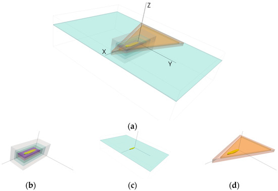
Figure 2.
Example of domain refinements (a), near field region (b), anisotropic free-surface (c) wave pattern refinements (d).
From a theoretical point of view, the speed profile module across the boundary layers changes, starting from zero on the wall. Since the numerical domain is described through an unstructured mesh, a balance between the height of the first cell inside the boundary layer and the total number of cells inside the domain itself must be found. Following (52), for each wall inside the domain, the thickness (BL) of the theoretical boundary layer can be estimated.
where represents the significative dimension for the wall considered and is the dimensionless Reynolds number. Rather, the velocity profile inside the boundary layer has been described through the wall function approach because of the opportunity to model the near-wall region with reasonable computational effort required. Hence, by fixing the maximum value for the dimensionless wall distance, , to the value of 150, which is inside the theoretical limits () of the method as proposed in the “Notes on Computational Fluid Dynamics” book [26], it is possible to define the speed at a distance from the wall, as reported in (53).
The mesh obtained by applying the three types of refinements and by the characterizations for the boundary layer is shown in Figure 3a and in Figure 3b respectively.
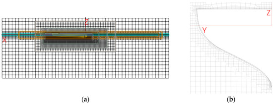
Figure 3.
Detail about symmetry plane mash (a) and transversal section for (b).
The parametric generation of the mesh features an additional control tool that enables the user to indirectly choose the total number of cells. To get a comparison among the numerical set-up, a mean value of 2.2 million cells has been retained as a good compromise among accuracy in calculation and computational effort for each simulation performed.
Considering that the flow around the hull and of its any potential appendance can be sufficiently described by the Reynolds-averaged approach, in which the Navier-Stokes equations [27] are treated as reported in (54).
where the average pressure fields, ρ the fluid density, μ its dynamic viscosity, represent the average velocity and the Reynolds stresses tensor. Among the turbulence models offered by the suite to achieve the tensor correctly described, the k-ω SST two-equation turbulence model (conservation equation and two transport equations) has been selected [28] based on its proficiency in accounting for the effect of convection and diffusion of turbulent energy through two variables (turbulent kinetic energy, , and turbulent dissipation rate, ). Whereas, to solve Equation (54), a finite volume method with cell-centered variables has been chosen for its robustness compared with free surface fitting methodology [29]. Inside the virtual domain, the free-surface divides the volume into two immiscible and isothermal fluids, water and air, respectively; for the described physics, the numerical solver is named interFOAM among the code libraries. As proposed by Hirt & Nichols [30] and tested in [31], the volume of fluid (VoF) approach has been selected to describe the interface effects among the two fluids. In this methodology, an indicator function can define the percentage of water inside each cell based on the variation between zero (all air) and one (all water), meaning that the value of 0.5 stands for the free-surface. Since the virtual towing tank calculation for a bare or a fully appended hull is expected to reach a steady state, among the code libraries the Local Time Step (LTS) approach has been selected. In this kind of approach, the time to reach the convergence is minimized because the time step is not constant among the cells inside the domain; indeed, considering the cells size changes, as reported in (55), the time step can be arranged to the minimum value inside each cell based on the local Courant number.
where is the local time step and is the characteristic dimension of the cell in the flow direction and is the flow speed in the flow direction.
The computational domain consists of a parallelepiped parametric box. The origin of the reference system is fixed at the intersection of the aft perpendicular of the model inside the domain and the free surface on the trace of the longitudinal symmetry plane of the ship. A right-had reference system is fixed on that origin with the x-axis (intersection of the free-surface and the symmetry plane) positive towards the bow, the y-axis (on the free-surface and perpendicular to the symmetry plane) positive among the left side of the model and the z-axis (perpendicular to the free-surface) positive upward. Since the ship symmetry, it is possible to split the whole domain into two identical domains and analyze one of them to reduce the computational effort; once the simulation has finished, it is possible to replicate the data for the other part. This kind of approach reduces considerably the computational effort but loses some asymmetrical phenomena such as von Kármán vortex street which are, however, considered negligible for the quantities of interests. Therefore, all the computations were performed with two degrees of freedom (one for sinkage and one for trim) to better reproduce the physics of the problem (a mesh morphing approach has been implemented to adapt the mesh for the check for the equilibrium of forces and momentum among bouncy and displacement, tested, with an iterative approach, four time in the simulation, respectively after 2000, 7000, 12,000 and 17,000 iterations).
Once the calculation reaches the convergence criteria, it is possible to perform the so-called post-processing analysis. For this particular kind of study (where several simulations performed with the same numerical set-up have been performed at model scale to be compared with an equal number of experimental tests), the history of the signal of the total resistance, , the frictional resistance, , and the pressure one, , deserves particular attention. For each simulation and with the respect to define a representative value for each one of them, the following four step work-flow has been created: step 1, graphical analysis to assess if a stabilized ratio has been achieved; step 2, low-pass filtration for the representative final part of the signal (last 5000 iterations) to neglect the numerical noise, where present; step 3, comparison among the standard deviation calculated for the two signals obtained to check for the agreement among them; step 4, evaluation for the representative value of the filtered signal. An example of the results from a CFD calculations are reported on Figure 4: on top-side the signals of forces (, and ) with the trace of the equilibrium check (the light blue triangles) and the stabilized zone for signals are shown for a single model hull (Figure 4a) along with the stabilized , its filtered signal () and representative value on bottom-left (Figure 4b); while the equilibrium checks for trim and sinkage are shown in bottom right (Figure 4c). For each model, CFD simulations have been performed at different speeds to reproduce the EFD experience.
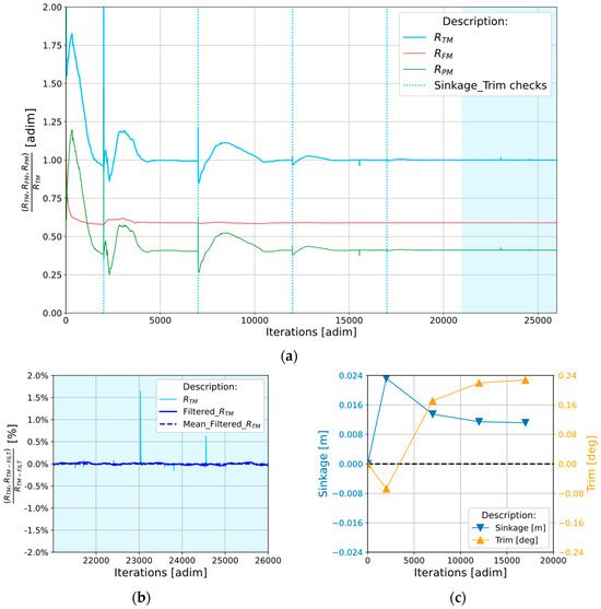
Figure 4.
Results from a CFD calculation for a model hull: , , (a) along with the (b) and the trim and sinkage (c).
Bozzo et al. [32] proposed to assess the virtual towing tank accuracy through a comparison between an EFD database and the CFD calculations. In the current work, two hulls (Hull_A and Hull_B) have been selected; their shapes and wave patterns for a single speed are shown for Hull_A in Figure 5a,b while, for Hull_B in Figure 5c,d, respectively.
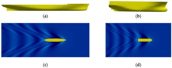
Figure 5.
Examples of two 3D hulls representation (a,b) and wave patterns (c,d) at the same advance speed (.
The two hulls have been considered in order to carry out the V&V procedure for the total resistance and addressing in an in-depth analysis of the dependency of on speed change and on the percentual deviation of the error, , among EFD results and CFD calculations, evaluated through (56), with a particular focus on its sensitivity to this kind of approach implemented to estimate it.
The main characteristics of the hulls are listed in Table 2.
Table 2.
Main geometrical and dynamical characteristics for the two hulls (Hull_A and Hull_B) used to perform the VVUA assessment.
Hull_A and Hull_B have been tested at different speeds (respectively three and four) and for each one with a different number of cells for a total number of 72 simulations. Because of the presence of a scatter in results and to check if this scatter is due to the presence of the dynamic attitude, further simulations have been performed with the attempt to analyze the uncertainty in results connected with the trim and the sinkage for the model; hence, considering Hull_B, two speeds are considered and other simulations have been performed in fix trim and sinkage configuration, identify through Hull_B-3* and Hull_B-4*, respectively. Table 3 reports all the details of this analysis; an attempt to bound the maximum difference among results, considering the concept of bounding uncertainty for the cases where an oscillatory convergence has been achieved among results (16), is present in the fourth column. These results seem to show a weak trend varying the speed; in fact, a positive dependence along with the speed is present for Hull_B rather a negative dependence for Hull_A exists but further investigations need to be performed.
Table 3.
Details about the 72 simulations used for Verification analysis on Hull_A and Hull_B; the number of cells is referred to half domain.
4. Results for Verification and Validation (V&V)
The V&V analysis can be split into three steps: the first consists in performing the simulations, while the second one deals with the numerical uncertainty assessment and in the last one the numerical results are compared with the experimental data available. In the following paragraphs details for each step will be provided.
Considering the cases labelled Hull_B-3 and Hull_B-4, where eight simulations have been performed for each case, the results aren’t into an asymptotic range. In particular, considering the versus a finer mesh topology (negative growth rate of cells, defined as and supposed finer than ), results exhibit a pattern which doesn’t allow finding a curve passing thought all of them and therefore, the asymptotic range seems not to be achieved, as shown in Figure 6a for Hull_B-3 and in Figure 6b for Hull_B-4.
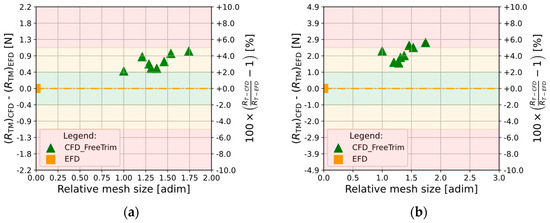
Figure 6.
Mesh independence analysis in free trim and sinkage condition (two degree of freedom) (a) on Hull_B-3 at and (b) on Hull_B-4 at .
Similar results have been achieved in all the other cases reported in Table 3, and considering that has a direct dependency on the trim, a possible way to reduce the obtained noise shown by the results, consists of performing simulations with a fixed value for trim and sinkage. Hence, for the two speeds identified by the labels Hull_B-3 and Hull_B-4, other simulations (labelled as Hull_B-3* and Hull_B-4*) have been run at fixed trim and sinkage conditions, considering the attitudes output from the two finer simulations. Figure 7 shows the results for the simulations performed in this configuration, in particular Figure 7a deals with Hull_B-3* and Figure 7b with Hull_B-4*, respectively.

Figure 7.
Mesh independence analysis in fix trim and sinkage condition (zero degree of freedom) (a) on Hull_B-3* at and (b) on Hull_B-4* at .
As shown in Figure 8a, by comparing results for Hull_B-3 (green triangles for free trim and sinkage) and Hull_B-3* (green star markers for fixed trim and sinkage), in both numerical configurations a similar behavior varying the mesh size is achieved with a sort of shifting, however nothing significant emerges by fixing the trim and sinkage. This demonstrates that the obtained noise in the solution is not primarily connected to the dynamic attitude. Nevertheless, the same considerations can be valid even for the comparison among Hull_B-4 and Hull_B-4*, as shown in Figure 8b; for this last case, several simulations have been performed to account for the numerical noise and great variation in the mesh size.
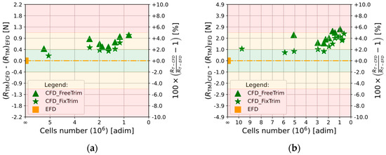
Figure 8.
Mesh independence analysis in fix trim and sinkage condition (stars markers) versus the free trim condition (triangular markers) (a) on Hull_B-3 alongside Hull_B-3 * at and (b) on Hull_B-4 alongside Hull_B-4* at .
4.1. Verification
A minimum of six simulations is available for each of the nine test cases, as reported in Table 3. Given the availability of this number of results, different kinds of theoretical approaches to assessing numerical uncertainty can be investigated. In this work, dealing with unstructured mesh and with a not constant grid refinement factor, it is possible to apply the theoretical procedure in several ways because of a minimum number of three simulations is required for Celik’s and Richarson’s generalized expansion methods (as proposed by Stern) rather a minimum number of four in Eça and Hoekstra’s one. Therefore, considering the case Hull_B-4* where 13 solutions (S = 13) are available and applying formulation (57) for 3 solutions (m = 3) and for 5 solutions (m = 5), the numerical available combinations are 286 and 1287 respectively [33].
By managing the possible combinations and comparing the available methodology to find a way to achieve , four approaches will be described in following, considering results from Hull_B-3* and Hull_B-4*.
Firstly, all data available are used in Eça and Hoekstra’s methodology and a triplet of results from the coarsest, the medium and the finer mesh (4.8, 1.9 and 0.9 million cells, ratio of 2.52 and 2.11) are considered to run the remaining approaches proposed by Celik, Stern, Xing and Stern. Considering Hull_B-3*, the effective order of accuracy, , presents an appreciable difference among the cases from the theoretical one, , except for Eça et al. methodology. Even for the numerical uncertainty, , values change, and this difference results from the approach and the correction proposed for the results (the four kinds of approach listed are: , , and 3 factors). For the case considered, and by changing the corrections, Celik and Stern give similar value for the uncertainty; its order of magnitude is close to 0.05 compared with the remaining cases where a similar value has been registered for the uncertainty. Finally, considering the percentage difference among the extrapolated values, all the methodologies are in good agreement with a maximum difference of 1.76%. Considering Hull_B-4*, similar considerations hold for the effective order of accuracy, , meanwhile, when considering the numerical uncertainty, , Eça et al. presents a different value, close to ten times compared with the other approaches. By looking at the scatter of data, Figure 7b and Figure 8b, it seems that the numerical noise for the 13 simulations may cause an increase in the uncertainty value, while it remains true that the extrapolated value for an infinite number of cells is the closest (among all the methodologies) to the EFD value. The numerical results for Hull_B-3* and Hull_B-4* (listed as H_B-3* and listed as H_B-4*) are reported in Table 4.
Table 4.
Mesh independence analysis first approach for Hull_B-3* and Hull_B-4* (fix trim and sinkage configuration) with different methodologies (number of cells for half domain Hull_B-3*: 4.8 M, 1.9 M, 0.9 M; number of cells for half domain Hull_B-4*: 9.7 M, 1.9 M, 0.6 M).
Considering the available data, it is possible to choose a triplet of results among the cases with a refinement factor close to 1.3, as suggested by Celik [8], upon which all the proposed methodologies, except for Eça et al. where all results are considered, can be applied. With respect to Hull_B-4*, three possible combinations come out from the results. Considering results from the semi-domains, in the first case (9.7, 5.0 and 2.4 million cells, ratio of 1.24 and 1.28) and in the second one (2.4, 1.0 and 0.6 million cells, ratio of 1.30 and 1.21), a divergence condition (R > 1) has been found and nothing can be established about uncertainty; while, in the last case (5.0, 2.4 and 1.0 4 million cells, ratio of 1.28 and 1.30), an oscillatory convergence (R < 0) occurs and it is possible to bound the numerical uncertainty (9) among the value of 1.24% normalized on the EFD. Based on Hull_B-3*, the lonely possible combination (4.8, 2.3 and 0.9 million cells, ratio of 1.26 and 1.35) leads to a monotonic convergence (R = 0.37). Similarly to the results obtained by the first approach, even in this case, the numerical uncertainty can be split into two groups, as shown in Table 5: a lower value from Celik and Stern theory and a higher one from the other approaches.
Table 5.
Mesh independence analysis second approach for Hull_B-3* (fix trim and sinkage configuration) with different methodologies (number of cells for half domain: 4.8 M, 1.9 M, 0.9 M).
Because of the presence of scatter distribution among solutions, the uncertainty estimation through a representative extrapolated function is highly affected by this variability. These fluctuations relate to the numerical noise in results and appear to be driven mainly by the unstructured mesh refinement approach, while the variation for trim and sinkage seems to be one order of lower magnitude. So, the fluctuations in results aren’t representative of a mesh refinement variation but rather of numerical noise and highly affect the uncertainty estimation. To account for this noise, a trend in results can be achieved by means of a selection of data among the available results, as described below. Firstly, starting from a scatter distribution, a second order function (with , and unknown coefficients) has been settled to minimize this difference through the Lest Square Root method (LSR). Secondly, the standard deviation () has been calculated considering the difference among each single data point and the curve in the respect of the . Thirdly, an interval with a symmetric interval of ± centered on the fit curve has been generated. Hence, fixed the curve along with the defined interval, a comparison check has been performed and if a generic point lies outside this boundary, the outlier condition occurs, and the point has to be neglected. Finally, considering the selected data, a new numerical uncertainty quantification has been performed. Based on a standard deviation of 25.11% for Hull_B-4*, the solutions considered moved from 13 to 8 and 5 are considered as outliers. In Figure 9a is reported a graphical overview of the distance among each data (identified by the stars and with colors connected with the mesh size) to the curve fit (which coincides with the trace of the bisector) for the case described and if the points lie in the red fields, the outlier condition occurs. While, in Figure 9b a comparison among the two cases (Hull_B-4*, red objects in the graph and Hull_B-4*_Filtered, green objects) has been reported along with the uncertainty values considering Eça and Hoekstra’s methodology.
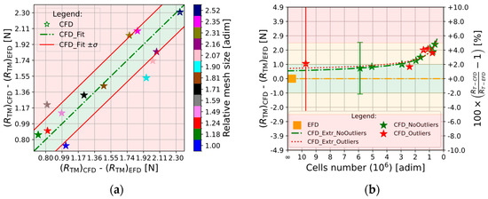
Figure 9.
Mesh independence analysis outlier verification for Hull_B-4*. (a) Core alongside outliers results inside the green and red field respectively; (b) Raw data fit curve (Hull_B-4*, red colors) versus the filtered and fitted one (Hull_B-4*_Filtered, green colors).
As expected, considering Hull_B-4*_Filtered, the value of decreases, (eventually halving) ranging from 9.81% for the first case to 3.53% for the second one within a difference of 0.62% has been found for the extrapolated values for the two configurations. This approach can be performed only with Eça and Hoekstra’s methodology and gives value for the numerical uncertainty that is closer to the one obtained by bounding it through the formula for the oscillatory convergence, as reported in (16), because somehow addresses the noise in results. Moreover, this noise can lead to the outlier condition even when a result comes from a simulation performed with a high number of cells, which is something incorrect from a theoretical point of view, but the noise affects all the solutions without regard for the discretization. Results for all the other methodologies are reported in Table 6; it could be argued that, considering the value of , even Stern and Xing account for a decrease rather the other methodologies assess an increase while looking at the extrapolated values, in all the other methodologies a decreased difference is assessed.
Table 6.
Mesh independence analysis third approach for Hull_B-4*_Filtered (fix trim and sinkage configuration, filtered data) with different methodologies (number of cells for half domain: 5.8 M, 1.9 M and 0.6 M).
Regarding the assessment of the numerical uncertainty, , considering the robustness and applicability of the proposed methodology, it is possible to perform another kind of analysis. In details, with the respect to a growth rate of cells not less than 1.2, and considering the case Hull_B-4* where 13 solutions are available, it is possible to select a group of results and try to assess their numerical uncertainty; thus, considering three and five solutions, a total number of 40 and 20 combinations has been considered for Celik’s, Stern’s approaches and Eça and Hoekstra’s one respectively. To compare the solutions with the attempt to define a general trend and any correlations, the x-axis (where the extrapolated value for the total resistance, , the order of accuracy, and the numerical uncertainty, are considered) has been divided in bins to count for the concurrencies in that range. With respect to the 3 solutions methodologies and considering to the types of convergence, the numerical uncertainty can be evaluated for 22 cases on 40 (55%) because of their monotonic convergence. Consequently, the assessments for , and will be carried out considering only the cases where monotonic behavior has been achieved. In Figure 10a,c,e Stern’s and Celik’s approaches are shown each considered on its own. With the respect of the extrapolated value for , most of the cases (close to 30%) gives quite the same value; while looking at the order of accuracy, nothing in particular comes out because of the scatter in data (the probability of occurrence is quite the same along the cases tested and its values aren’t so close to the value of two, which represents the theoretical order of accuracy). Lastly, considering , most of the cases presents a value which is less than 2% and Celik’s approach gives for about 70% of occurrences a value lower than 1%. Considering the 20 cases for the 5 solutions, for each one of them a value for , and has been obtained and therefore it is possible to get a 100% of efficiency in defining the values of interest. By analyzing the results, instead, it is possible to get information about their general behavior as shown by Figure 10b,d,f where the 20 combinations for 5 results are reported and compared with all solutions (red vertical line). In particular, considering , most of result (percentage greater than 40%) converge to a quite common value which is close to the one obtained by considering all the 13 solutions, while, considering , most of combinations lies within the range of +1% to +8% and finally, looking at , most of combinations (approximately 70%) gives a value which is close to the theoretical one.
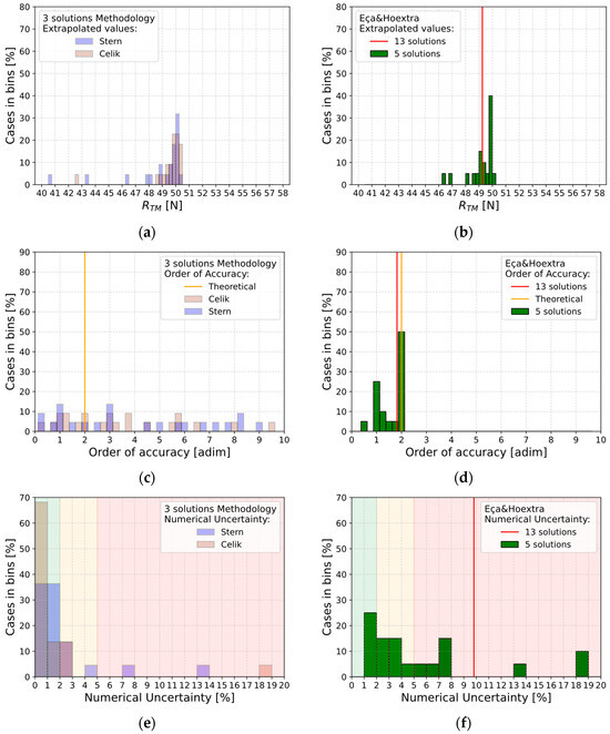
Figure 10.
Verification analysis results for with the three solutions methodologies proposed by Stern and Celik (considered individually, (a,c,e)), and with the five-solutions methodology proposed by Eça and Hoekstra (b,d,f).
Considering the scatter in results for by varying the combinations, as illustrated by Figure 11a and considering the value of , as shown in Figure 11b, it is evident how the value of the order of accuracy can influence the value for the numerical uncertainty. More in detail, a value for which is smaller than 0.5 compared with the theoretical one, leads to an uncertainty considerably higher (for some cases an order of magnitude higher has been registered).
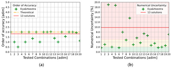
Figure 11.
Variation for the order of accuracy (a) and for the numerical uncertainty (b) obtained by changing the tested combination of five-solutions methodology proposed by Eça and Hoekstra.
Therefore, the analysis is limited to cases where the order of accuracy falls within the range of 1.5 to 2. This selection leads to the results presented in Figure 12a–d. In details, with the respects for , about 70% of results tends to converge to a quite common value which is close to the one obtained by considering all the 13 solutions, while, considering , the value is lower than the one obtained considering all , but its variations lays on the range from 1% to 6% with a probability to be lower than 3% for 60% of cases. Consequently, considering a general application for the Eça and Hoekstra’s methodology, when the value for tends to be smaller than 1.5 or bigger than 2, further investigations have to be performed; in particular, with the respect to the value of the numerical uncertainty , an overestimation can occur, while considering the extrapolated value for the resistance , the order of accuracy affects it with a lower influence compared with .
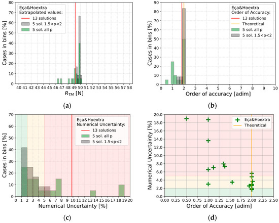
Figure 12.
Results for along with the five-solutions methodology proposed by Eça and Hoekstra when considering an order of accuracy between 1.5 and 2 (d).
Therefore, it is evident how the choice of data plays a crucial rule in the uncertainty prediction and moreover, even the extrapolated value can be affected by the choice especially when addressing all the methodologies with the exception of Eça and Hoekstra, where a higher level for is registered, but with an invariant value for the extrapolated value.
4.2. Validation
Strictly speaking, as mentioned previously, since the uncertainty analysis for the EFD results is not available, from a theoretical point of view the V&V procedure cannot be finalized due to the lack of . To partially overcome this limitation, the variation of the standard deviation for the resistance coefficient in a comparative test performed by several towing tanks can lead to accounting for the order of magnitude for . Indeed, as stated in the Proceedings of 28th ITTC [34], it is possible to assess the standard deviation for a group of tests performed by several towing tanks for exactly the same model hull (DTMB 5415), tested at different speeds and in two different model length ( for the smaller and for the bigger). Therefore, a rough order-of-magnitude estimate of for another model hull with different , can be derived through a double interpolation (speed and length) among the available data. Indeed, fixing a model length (), it is possible to create a line with a representative standard deviation; considering the red and blue lines as the results of the 28th ITTC (held in Wuxi), and the green dash-dot line as the output of the interpolations, results for Hull_B-3* () and Hull_B-4* () are respectively shown in Figure 13a,b, where the rough order of magnitude for is 1.53 for the first one and 2.04 for the second one.
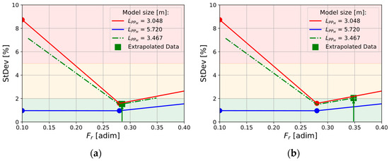
Figure 13.
Rough order-of-magnitude estimate of for Hull_B-3* (a) and Hull_B-4* (b).
Given the formulations for the validation procedure, and by considering all the numerical approaches along with the bounding approach one, results for validation uncertainty, , reported into Table 7 shows a good agreement with the virtual towing tank accuracy as found in Bozzo et al.’s work [32]. Moreover, from data it comes out that the speed variation doesn’t affect the uncertainty estimation because of the absence of a clear, positive or negative, trend among results.
Table 7.
Simulations performed for Verification analysis with different approaches; for the three solutions methodologies.
5. Conclusions
Current study shows results related the verification and validation procedures applied to the resistance prediction for model-scale hulls. Regarding verification procedures, four different theoretical methodologies have been investigated to evaluate numerical uncertainty. Each method includes Richardson extrapolation and handles higher-order terms in the power series expansion differently. These approaches can be grouped into two families:
- Three solutions methodologies, where three results are required to begin the analysis.
- Eça and Hoekstra methodology, where at least four results are required to perform the assessment.
In terms of validation, due to the lack of experimental uncertainty data, the process cannot be formally completed from a theoretical standpoint. However, general considerations can still be discussed.
To compare the methodologies, two hulls were tested at different speeds. For the three solutions approaches, numerical uncertainty, , can be evaluated only if monotonic convergence is achieved. Among the cases studied, this condition was met in 55% of instances. When uncertainty could be calculated, Celik’s method yielded values below 1%, while Stern’s approach typically produced values under 2% While considering Eça and Hoekstra’s approach, where at least four solutions are required, the value for numerical uncertainty can be always obtained. The analysis shows that the estimated uncertainty values were generally higher than those obtained using the three-solution methods. This outcome is expected due to numerical noise between solutions, likely caused by the use of unstructured meshes in the simulations. When multiple datasets are considered, this noise can significantly affect uncertainty estimates, leading to overestimation.
To partially mitigate the noise in results, the order of accuracy obtained from mesh refinement analysis can serve as an indicator of reliability. If the computed order deviates significantly from the theoretical value (), particularly falling below 1.5 or higher than 2, the associated uncertainty is likely overestimated, and further investigation is recommended.
All the methodologies proposed, when comparable (especially in cases of monotonic convergence), yield similar extrapolated resistance predictions, , while, considering the numerical uncertainty, the estimation performed with Eça and Hoekstra’s approach is usually higher compared with the Celik’s and Stern’s methodologies, where a mean global value of 6.65%, 0.39% and 2.01% has been respectively recorded.
Compared to the three-solution methods, the four-solution methodology demonstrates greater robustness and reliability. It consistently provides results for extrapolated values, order of accuracy, and numerical uncertainty. Out of 40 cases analyzed using the three-solution methods, only 22 yielded usable results (a success rate of 55%), whereas all 20 cases evaluated with the four-solution approach were successful (100% success rate). Based on these findings and the data used in the present study, Eça and Hoekstra’s approach is preferable due to its robustness. To partially mitigate the overestimations observed, the order of accuracy obtained by the mesh independence analysis can be used an index for the reliability of the numerical uncertainty estimation and when its value decrease below 1.5 further investigations needs to be carried out.
Based on the findings of the present research, future work will apply the proposed methodology to additional hull shapes tested at various speeds, aiming to build a statistical database. Once sufficient data are collected, general insights into uncertainty assessment will be extracted, allowing for evaluation of whether the proposed procedure remains valid or requires further refinement.
Author Contributions
Conceptualization, S.B. and D.V.; methodology, S.B.; software, S.B. and D.V.; validation, D.V. and S.M.; formal analysis, S.B.; writing—original draft preparation, S.B.; writing—review and editing, S.B., D.V. and S.M.; supervision, D.V. and S.M. All authors have read and agreed to the published version of the manuscript.
Funding
This research received no external funding.
Data Availability Statement
The original contributions presented in this study are included in the article.
Conflicts of Interest
The authors declare no conflicts of interest.
Abbreviations
The following abbreviations are used in this manuscript:
| American Institute of Aeronautics and Astronautics | |
| Apparent order of accuracy | |
| Boundary layer | |
| Breadth at design WL, Maximum moulded [m] | |
| Block coefficient [adim] | |
| Computational Fluid Dynamics | |
| Correction Factor | |
| Draught at midship | |
| Error | |
| Error estimate (numerical) | |
| Error contribution for grid size | |
| Error contribution for the iteration number | |
| Error contribution for the step | |
| Error contribution for other parameters | |
| Experimental Fluid Dynamics | |
| Factor of safety | |
| Froude number | |
| Grid Convergence Index | |
| Grid ratio parameter | |
| International Towing Tank Conference | |
| Length of waterline [m] | |
| model value | |
| Modelling Uncertainty | |
| Modelling simulation error | |
| Number of cells inside the domain | |
| Numerical Uncertainty | |
| Numerical simulation error | |
| Numerical simulation error estimate of sign and magnitude | |
| Open Field Operation And Manipulation | |
| Ratio of solution change | |
| Resistance of advance for the model evaluated by CFD [N] | |
| Resistance of advance for the model evaluated by EFD [N] | |
| Reynolds number [adim] | |
| Scale ratio [adim] | |
| Simulation Uncertainty | |
| Simulation correct uncertainty | |
| Simulation error | |
| Simulation result | |
| Simulation correct value | |
| Simulation 1 value, Simulation 2 value, …, Simulation n value | |
| Solution extrapolated from solution 1 and solution 2 | |
| True value | |
| ∇ | Volume, displacement [m3] |
| Uncertainty | |
| Uncertainty Assessment | |
| Wetted surface area [m2] | |
| Verification and Validation | |
| Verification, Validation and Uncertainty Assessment |
References
- Lewis, E.V. Principles of Naval Architecture: Resistance, Propulsion and Vibration, 2nd ed.; Society of Naval Architects and Marine Engineer: Jersey City, NJ, USA, 1988; p. 5. ISBN 0-939773-01-5. [Google Scholar]
- History of ITTC. Available online: https://ittc.info/about-ittc/history (accessed on 15 September 2025).
- ITTC Quality System Manual Recommended Procedures and Guidelines. Register. Available online: https://ittc.info/media/11718/0_0.pdf (accessed on 15 September 2025).
- Runchal, A.K. Evolution of CFD as an engineering science. A personal perspective with emphasis on the finite volume method. Comptes Rendus Mécanique 2022, 350, 233–258. [Google Scholar] [CrossRef]
- Larsson, L.; Stern, F.; Visonneau, M. CFD in Ship Hydrodynamics—Results of the Gothenburg 2010 Workshop. In MARINE 2011, IV International Conference on Computational Methods in Marine Engineering; Springer: Dordrecht, The Netherlands, 2013; pp. 237–259. [Google Scholar] [CrossRef]
- Lopes, R.; Eslamdoost, A.; Everyd Bensow, R.; Ponkratov, D.; Kömpe, A.; Geremia, P.; Birant Pekküçük, Ç.; Aydin, C.; Villa, D.; Ntouras, D.; et al. A Summary of the Lucy Ashton Resistance Prediction Workshop. In Proceedings of the MARINE 2025, XI International Conference on Computational Methods in Marine Engineering, Edinburgh, UK, 23–25 June 2025; Preprint submitted to Ocean Engineering: Amsterdam, The Netherlands, 2025. [Google Scholar]
- Islam, H.; Guedes Soares, C. Uncertainty analysis in ship resistance prediction using OpenFOAM. Ocean. Eng. 2019, 191, 105805. [Google Scholar] [CrossRef]
- Celik, I.; Ghia, U.; Roache, P.J.; Freitas, C.; Coloman, H.; Raad, P. Procedure for Estimation and Reporting of Uncertainty Due to Discretization in CFD Applications. J. Fluids Eng. 2008, 130, 078001. [Google Scholar] [CrossRef]
- Stern, F.; Wilson, R.; Coleman, H.; Paterson, E. Comprehensive Approach to Verification and Validation of CFD Simulations—Part 1: Methodology and Procedures. J. Fluids Eng. 2001, 123, 793–802. [Google Scholar] [CrossRef]
- Xing, T.; Stern, F. Factors of Safety for Richardson Extrapolation; IIHR—Hydroscience & Engineering: Iowa City, IA, USA, 2010. [Google Scholar] [CrossRef]
- Eça, L.; Hoekstra, M. A procedure for the estimation of the numerical uncertainty of CFD calculations based on grid refinement studies. J. Comput. Phys. 2014, 262, 104–130. [Google Scholar] [CrossRef]
- Diez, M.; Broglia, R.; Durante, D.; Olivieri, A.; Campana, E.; Stern, F. Validation of Uncertainty Quantification Methods for High-Fidelity CFD of Ship Response in Irregular Waves. In Proceedings of the 55th AIAA Aerospace Sciences Meeting, Grapevine, TX, USA, 9–13 January 2017. [Google Scholar]
- ITTC Quality System Manual Recommended Procedures and Guidelines. Uncertainty Analysis in CFD Verification and Validation, Methodology and Procedures 7.5-03-01-01. Available online: https://www.ittc.info/media/11950/75-03-01-01.pdf (accessed on 15 September 2025).
- Sadrehaghighi, I. Computational Error and Uncertainty Quantification in CFD; CFD Open Series: Annapolis, MD, USA, 2021. [Google Scholar] [CrossRef]
- American Institute of Aeronautics and Astronautics (AIAA). Guide for the Verification and Validation of Computational Fluid Dynamics Simulations; AIAA G-077-1998; American Institute of Aeronautics and Astronautics: Reston, VA, USA, 1998. [Google Scholar]
- Coleman, H.W.; Steele, W.G. Experimentation and Uncertainty Analysis for Engineers; Wiley: Hoboken, NJ, USA, 1999. [Google Scholar]
- Oberkampf, W.L.; Trucano, T.G. Verification and validation in computational fluid dynamics. Prog. Aerosp. Sci. 2002, 38, 209–272. [Google Scholar] [CrossRef]
- Richardson, L.F.; Gaunt, J.A., VIII. The deferred approach to the limit. Philos. Trans. R. Soc. Lond. Ser. A Contain. Pap. Math. Phys. Character 1997, 226, 299–361. [Google Scholar] [CrossRef]
- Wilson, R.; Stern, F.; Coleman, H.; Paterson, E. Comprehensive Approach to Verification and Validation of CFD Simulations—Part 2: Application for Rans Simulation of a Cargo/Container Ship. J. Fluids Eng. 2001, 123, 803–810. [Google Scholar] [CrossRef]
- Huang, S.; Jiao, J.; Guedes Soares, C. Uncertainty analyses on the CFD–FEA co-simulations of ship wave loads and whipping responses. Mar. Struct. 2022, 82, 103129. [Google Scholar] [CrossRef]
- Lakatoš, M.; Mancini, S.; Niazmand Bilandi, R.; Tabri, K. Verification and validation of hard-chine hull performance in calm water: Effects of numerical setups and hull configurations. Ocean. Eng. 2025, 329, 121056. [Google Scholar] [CrossRef]
- Coleman, H.; Stern, F.; Di Mascio, A.; Campana, E. The Problem with Oscillatory Behavior in Grid Convergence Studies. J. Fluids Eng. 2001, 123, 438–439. [Google Scholar] [CrossRef]
- Roache, P.J. Verification and Validation in Computational Science and Engineering; Hermosa Publishers: Socorro, NM, USA, 1998. [Google Scholar]
- Villa, D.; Furcas, F.; Pralits, J.; Vernengo, G.; Gaggero, S. An Effective Mesh Deformation Approach for Hull Shape Design by Optimization. J. Mar. Sci. Eng. 2021, 9, 1107. [Google Scholar] [CrossRef]
- ITTC Quality System Manual Recommended Procedures and Guidelines. Practical Guidelines for Ship Resistance CFD. 7.5-03-03-04. Available online: https://www.ittc.info/media/9775/75-03-02-04.pdf (accessed on 15 September 2025).
- Greenshields, C.; Weller, H. Notes on Computational Fluid Dynamics: General Principles; CFD Direct Ltd.: Reading, UK, 2022. [Google Scholar]
- Gaggero, S.; Villa, D.; Viviani, M. The Kriso container ship (KCS) test case: An open source overview. In Proceedings of the MARINE 2015—VI International Computational Methods in Marine Engineering, Rome, Italy, 15–17 June 2015; CIMNE: Barcelona, Spain, 2015; pp. 735–749. [Google Scholar]
- Chiroșcă, A.; Rusu, L. Comparison between Model Test and Three CFD Studies for a Benchmark Container Ship. J. Mar. Sci. Eng. 2021, 9, 62. [Google Scholar] [CrossRef]
- Leroyer, A.; Wackers, J.; Queutey, P.; Guilmineau, E. Numerical strategies to speed up CFD computations with free surface—Application to the dynamic equilibrium of hulls. Ocean. Eng. 2011, 38, 2070–2076. [Google Scholar] [CrossRef]
- Hirt, C.W.; Nichols, B.D. Volume of fluid (VOF) method for the dynamics of free boundaries. J. Comput. Phys. 1981, 39, 201–225. [Google Scholar] [CrossRef]
- Bozzo, S.; Villa, D. A Fast Numerical Procedure to Design the Shaftline Struts. In Proceedings of the 13th Symposium on High Speed Marine Vehicles (HSMV), Naples, Italy, 23–25 October 2023; IOS Press Ebooks: Amsterdam, The Netherlands, 2023; pp. 42–52. [Google Scholar] [CrossRef]
- Bozzo, S.; Ferrando, M.; Villa, D. Analysis of the virtual towing tank accuracy by means of a new EFD database. In Proceedings of the 21st International Conference on Ships and Maritime Research (NAV 2025), Messina, Italy, 18–20 June 2025; IOS Press Ebooks: Amsterdam, The Netherlands, 2025; pp. 241–251. [Google Scholar]
- Levin, O. Discrete Mathematics: An Open Introduction, 4th ed.; Oscar Levin: Greeley, CO, USA, 2025; Available online: https://discrete.openmathbooks.org (accessed on 15 September 2025).
- ITTC. The Resistance Committee. In Proceedings of the 28th ITTC, Wuxi, China, 17–22 September 2017; Test Data. Volume I. Available online: https://www.ittc.info/media/7797/4-resistance-committee.pdf (accessed on 15 September 2025).
Disclaimer/Publisher’s Note: The statements, opinions and data contained in all publications are solely those of the individual author(s) and contributor(s) and not of MDPI and/or the editor(s). MDPI and/or the editor(s) disclaim responsibility for any injury to people or property resulting from any ideas, methods, instructions or products referred to in the content. |
© 2025 by the authors. Licensee MDPI, Basel, Switzerland. This article is an open access article distributed under the terms and conditions of the Creative Commons Attribution (CC BY) license (https://creativecommons.org/licenses/by/4.0/).