A Gaussian-Process-Based Model Predictive Control Approach for Trajectory Tracking and Obstacle Avoidance in Autonomous Underwater Vehicles

Abstract

To achieve the efficient and precise control of autonomous underwater vehicles (AUVs) in dynamic ocean environments, this paper proposes an innovative Gaussian-Process-based Model Predictive Control (GP-MPC) method. This method combines the advantages of Gaussian process regression in modeling uncertainties in nonlinear systems, and MPC’s constraint optimization and real-time control abilities. To validate the effectiveness of the proposed GP-MPC method, its performance is first evaluated for trajectory tracking control tasks through numerical simulations based on a 6-degrees-of-freedom, fully actuated, AUV dynamics model. Subsequently, for 3D scenarios involving static and dynamic obstacles, an AUV horizontal plane decoupled motion model is constructed to verify the method’s obstacle avoidance capability. Extensive simulation studies demonstrate that the proposed GP-MPC method can effectively manage the nonlinear motion constraints faced by AUVs, significantly enhancing their intelligent obstacle avoidance performance in complex dynamic environments. By effectively handling model uncertainties and satisfying motion constraints, the GP-MPC method provides an innovative and efficient solution for the design of AUV control systems, substantially improving the control performance of AUVs.

1. Introduction

As technological capabilities have rapidly progressed, enabling the deeper exploration of the ocean realm, autonomous underwater vehicles (AUVs) have proven to be indispensable tools in unlocking the mysteries of the deep. These unmanned, cable-free underwater vehicles are equipped with the requisite instrumentation, including sonar, a Doppler Velocity Log (DVL), and an Inertial Measurement Unit (IMU), and rely on embedded control computers and autonomous control software to execute pre-defined navigation tasks. Due to their exceptional underwater performance, adaptability, and mission-execution capabilities, AUVs have become vital assets in various applications, including marine resource exploration and development (Hong et al., 2021 [1]; Zhang et al., 2015 [2]), marine information monitoring (Sagala et al., 2011 [3]; Wang et al., 2021 [4]; Cong et al., 2023 [5]), marine reconnaissance (Tang et al., 2023 [6]), and rescue missions (Kirkwood, 2007 [7]; Thomas et al., 2021 [8]). These abilities have elevated AUVs to a prominent research focus in the field of ocean engineering globally (Curtin et al., 2005 [9]). As the demand for AUV applications expands, these vehicles are being tasked with increasingly varied and complex roles. This evolution necessitates enhanced motion control systems that allow AUVs to fulfill human demands more effectively. However, achieving the precise control of AUVs is a formidable and vital challenge, attributed to factors like strong coupling, nonlinearity, and operational constraints (Xia et al., 2022 [10]; Gong et al., 2022 [11]; Wang et al., 2013 [12]).

Model Predictive Control (MPC) is an advanced control strategy capable of addressing the input and state constraints of a system in real-time, which emanate from its inherent physical and safety limitations. These constraints arise from the physical characteristics and safety limitations of the system and are widely present in all systems (Zhang et al., 2019 [13]). Contrary to traditional optimal control strategies that necessitate comprehensive optimization across the entire temporal domain, MPC enhances computational efficiency by focusing on localized optimizations within a predefined future timeframe. This method not only reduces computational complexity but also endows the control system with a predictive capability, allowing it to infer future dynamics based on current and impending control inputs.

Model Predictive Control (MPC) exhibits a distinct advantage in handling tasks that demand precise navigation and obstacle circumvention under various constraints, a feature that is well-evidenced in trajectory tracking and obstacle avoidance applications (Khodayari et al., 2015 [14]; Qiao et al., 2017 [15]; Peng et al., 2019 [16]) and obstacle avoidance (Cho et al., 2019 [17]; Trym et al., 2020 [18]; Zhang et al., 2022 [19]). Within the specialized context of AUVs, Bao et al. (2022 [20]) have pioneered an integrated control approach by amalgamating optimized MPC with Nonlinear Tilted Sliding Mode Control (NTSMC) and an adaptive Radial Basis Function Neural Network (RBF NN) compensator. This innovative method is designed to enhance the accuracy of dynamic trajectory tracking. This dual-loop system effectively mitigates constraints and external disturbances, ensuring both stability and robust performance, validated through Lyapunov stability analysis and extensive simulation under varied marine conditions.

Moreover, Oh and Sun explored the application of linear MPC in conjunction with line-of-sight (LOS) guidance for path-following control, utilizing quadratic programming to derive the control input, a method proven to be effective in simulations involving underactuated surface vessels (2010 [21]). Gao et al. (2016 [22]) presented a nonlinear MPC-based adaptive dynamic positioning control for fully driven underwater vehicles, enhancing system robustness and velocity tracking accuracy through neural network integration, with the efficacy demonstrated using the horizontal plane model of a Remotely Operated Vehicle (ROV).

However, the intensive computational demand of MPC can potentially affect the real-time performance of control systems. To address this, Wang et al. (2022) proposed a self-adaptive predictive control methodology utilizing least squares and Lagrange functions to decrease computational strain while improving system robustness and interference mitigation. Zhang et al. (2019 [13]) streamlined the MPC optimization process into a convex quadratic problem, facilitating online resolution and proving its trajectory tracking capability under external disturbances. However, the computational intensity of MPC can affect real-time control system performance, a challenge addressed by Wang et al. (2022 [23]) through a self-adaptive predictive control method using Lagrange functions and least squares algorithms, improving system robustness and reducing computational demands.

Further innovations include that of Song et al. (2017 [24]), who combined probabilistic policy search with MPC for enhanced decision-making in control systems, demonstrating success in agile drone navigation. Piotr et al. (2011 [25]) designed a ship course-keeping algorithm based on a knowledge base, which utilizes a set of input and output signals to obtain ship dynamics equations, thus avoiding the problems that arise when designing classical control algorithms for complex nonlinear ship models. Yao et al. (2018 [26]) improved MPC efficiency by adapting the weighting matrix based on error magnitude, enhancing control precision as verified in pool experiments. Uchihori et al. (2021 [27]) proposed an MPC-based AUV docking control system, employing a linear parameter variation (LPV) model and a time-varying Kalman filter to manage power flow disturbances.

Additionally, Maciejowski et al. (2013 [28]) introduced a fault-tolerant control method for Unmanned Aerial Vehicles (UAVs) combining the Gaussian process and MPC, with successful simulation outcomes. Hewing et al. (2017 [29]) developed an adaptive control approach for autonomous miniature race cars, leveraging the Gaussian process and chance-constrained formulations to account for model uncertainties. Collectively, these studies contribute significant insights and methodological advancements to the field of MPC, particularly in enhancing the control systems of AUVs and related autonomous platforms.

Appropriate modeling plays a crucial role in achieving high-precision control (Li et al., 2021 [30]). Gaussian process regression effectively addresses model uncertainty in nonlinear data fitting by estimating probability distributions, mitigating the influence of system noise. Leveraging this ability, this study employs a Gaussian-Process-based Model Predictive Control (GP-MPC) approach to control AUVs, aiming to guide the AUVs in achieving precise trajectory tracking within a three-dimensional spatial domain. The proposed method can be applied to Level 2 autonomous vehicles, which are partially automated (Khosrow-Pour et al., 2020 [31]). In addition to trajectory tracking tasks, we evaluate the AUV’s planar model for its proficiency in evading obstacles in static and dynamic environments. This method integrates a non-parametric Gaussian process model with MPC, constructing a robust controller with predictive capabilities. It is designed to address various challenges posed by the complex marine environment, such as model uncertainties, external disturbances, and constraints, thereby providing a theoretical foundation and technical support for achieving the high-precision motion control of AUVs.

The remaining sections of this paper are organized as follows: Section 2 details the procedure for establishing the kinematics and dynamics model of the AUV, while Section 3 presents the formulation of the Gaussian-process-based MPC controller for the AUV. Additionally, Section 4 elucidates the simulation of both trajectory tracking and obstacle avoidance tasks, demonstrating and analyzing the performance of the proposed GP-MPC approach. Finally, Section 5 provides concluding remarks and discussions regarding the research findings and potential future directions. Through this organization, the present study aims to develop an advanced control framework for AUVs, enhancing their navigation accuracy and robustness in complex environments, while exploring the potential applicability of the proposed methodology in the broader domain of autonomous system control.

2. Modeling of AUV

In the process of modeling and controlling AUVs, the establishment of coordinate systems, formulation of kinematic models, and development of dynamic models serve as pivotal elements that form the fundamental underpinning of achieving high-precision control in underwater environments. The accurate establishment of coordinate systems aids in comprehending and describing the AUV’s position and orientation in three-dimensional space. Kinematic models reveal the motion characteristics of the AUV, including velocity, direction, and attitude. Dynamic models further deepen our understanding of AUV behavior by accounting for various external forces and disturbances. This section delves into the modeling efforts across these three critical domains, providing the essential theoretical foundation for an in-depth exploration of AUV behavior.

2.1. Coordinate System Establishment

To accurately depict the spatial position and attitude of the AUV, it is imperative to establish appropriate coordinate systems. In this regard, this paper presents the establishment of two coordinate systems: the ground coordinate system, referred to as {G}, and the body coordinate system, denoted as {B}. In order to effectively determine the angular relationship between the {G} and {B} systems, the auxiliary north–east–down coordinate system ({NED}) is selected to represent the angular correlation between the {G} and {B} systems. The Euler angles, representing the angle between the corresponding axes of the {NED} system and the {B} system, are employed to describe the AUV’s attitude. It is important to note that the choice of rotation order for the Euler angles can yield varying coordinate system conversion relations.

The relationship among the three above-mentioned coordinate systems is depicted in Figure 1. The ground coordinate system establishes a reference point, denoted as $O$ on the Earth’s surface, serving as the coordinate origin, with the coordinate axes being stationary relative to the ground. Specifically, the $x$-axis aligns with the north pole, the $y$-axis aligns with the east direction, and the $z$-axis points downwards, normal to the Earth’s surface. The body coordinate system is typically established with the center of buoyancy of the AUV as the origin. The $x_b$-axis points forward, along the AUV’s longitudinal axis, the $y_b$-axis points towards the starboard of the AUV, and the $z_b$-axis is perpendicular to the $O_b-x_b{y}_b$ plane and points downward. The north–east–down coordinate system can be visualized as a ground coordinate system that moves in tandem with the AUV. Its origin remains fixed on the AUV and generally coincides with the origin of the body coordinate system. The orientation of the coordinate axes aligns with that of the ground coordinate system.

2.2. Kinematic Model Formulation

Building upon the previously established coordinate systems, the development of a kinematic model is crucial to comprehensively understand the motion characteristics of the AUV. According to the coordinate systems relationship outlined in Section 2.1, the {B} system can also be derived by sequentially rotating the $z_n$, $y_n$, and $x_n$ axes of the {NED} system in turn. By calculating the three corresponding rotation angles, which represent the yaw $\psi$, pitch $\theta$, and roll $\varphi$, respectively, the transformation relationship between the {B} system and the {NED} system can be established.

For the sake of simplicity and to facilitate the development of the model in the subsequent sections, let ${\mathit{\eta }}_1={[x,y,z]}^{\mathrm{T}}$ represent the position vector of the AUV in the {G} system, and ${\mathit{\eta }}_2={[\varphi ,\theta ,\psi ]}^{\mathrm{T}}$ represent the orientation vector of the AUV in the {G} system. Here, $x$, $y$, and $z$ represent the three Cartesian coordinates, while $\varphi$, $\theta$, and $\psi$ represent the three components of the AUV’s attitude, respectively. Furthermore, let ${\mathit{v}}_1={[u,v,w]}^{\mathrm{T}}$ and ${\mathit{v}}_2={[p,q,r]}^{\mathrm{T}}$ describe the linear velocity vector and angular velocity vector of the AUV in the {B} system. Specifically, $u$, $v$, and $w$ correspond to the translational velocity components along the $x_b$,$y_b$, and $z_b$ axis, while $p$, $q$, and $r$ represent the three rotational velocity components, respectively. Using these notations, the AUV kinematic equations can be expressed as follows:

$$\dot{\mathit{\eta }}=\mathit{J}\left({\mathit{\eta }}_2\right)\mathit{v}$$

(1)

$$\mathit{J}\left({\mathit{\eta }}_2\right)=\left[\begin{array}{cc}{\mathit{R}}^{3\times 3}& \mathit{O}\\ \mathit{O}& {\mathit{T}}^{3\times 3}\end{array}\right]$$

(2)

where $\mathit{\eta }$ and $\mathit{v}$ represent the compact form of the AUV state and velocity, which can be expressed as follows:

$$\mathit{\eta }={\left[{\mathit{\eta }}_1^{\mathrm{T}},{\mathit{\eta }}_2^{\mathrm{T}}\right]}^{\mathrm{T}}$$

(3)

$$\mathit{v}={\left[{\mathit{v}}_1^{\mathrm{T}},{\mathit{v}}_2^{\mathrm{T}}\right]}^{\mathrm{T}}$$

(4)

In Equation (2), matrix ${\mathit{R}}^{3\times 3}$ represents the translational velocity rotation matrix from the {B} system to the {G} system, while matrix ${\mathit{T}}^{3\times 3}$ denotes the rotational velocity rotation matrix from system {B} to system {G}. In addition, $\mathit{O}$ represents the zero matrix. These two matrices, ${\mathit{R}}^{3\times 3}$ and ${\mathit{T}}^{3\times 3},$ can be defined as follows:

$$\begin{array}{c}{\mathit{R}}^{3\times 3}=\left[\begin{array}{cc}\cos \psi \cos \theta & -\sin \psi \cos \varphi +\cos \psi \sin \theta \sin \varphi \\ \begin{array}{c}\sin \psi \cos \theta \\ -\sin \theta \end{array}& \begin{array}{c}\cos \psi \cos \varphi +\sin \varphi \sin \theta \sin \psi \\ \cos \theta \sin \varphi \end{array}\end{array}\right.\\ \left.\begin{array}{c}\sin \psi \sin \varphi +\cos \psi \\ -\cos \psi \sin \varphi +\sin \theta \sin \psi \cos \varphi \\ \cos \theta \cos \varphi \end{array}\right]\end{array}$$

(5)

$${\mathit{T}}^{3\times 3}=\left[\begin{array}{ccc}1& \sin \varphi \tan \theta & \cos \varphi \tan \theta \\ 0& \cos \varphi & -\sin \varphi \\ 0& \frac{\sin \varphi }{\cos \theta }& \frac{\cos \varphi }{\cos \theta }\end{array}\right]$$

(6)

According to Equation (6), when angle $\theta =\pm \pi ∕2$, using Euler angles to describe the AUV’s attitude results in singularity in matrix ${\mathit{T}}^{3\times 3}$ (Do and Pan, 2009 [32]). This singularity situation can render the kinematic equations unsolvable. Therefore, when formulating the control strategy, it becomes crucial to impose constraints on the AUV’s state to ensure that the pitch angle does not reach these critical values. Based on the preceding discussion, the development of the kinematic model plays a pivotal role in accurately characterizing the motion dynamics of the AUV. This provides us with a detailed understanding of how the AUV’s position and attitude change over time, offering critical insights into its behavior and capabilities.

2.3. Dynamic Model Development

Expanding upon the preceding kinematic modeling, the dynamic modeling of the AUV emerges as paramount for comprehensively capturing its motion characteristics. This includes the intricate interplay of external forces and allows for the formulation of effective control strategies. By considering the interplay between external generalized forces and AUV motion, the dynamic equations of the AUV can be derived using the Newton–Euler method, as demonstrated by Fossen (Fossen, 2011 [33]):

$$\mathit{M}\dot{\mathit{\nu }}+\mathit{C}\left(\mathit{v}\right)\mathit{v}+\mathit{D}\left(\mathit{v}\right)\mathit{v}+\mathit{g}\left(\mathit{\eta }\right)=\mathit{\tau }$$

(7)

In Equation (7), matrix $\mathit{M}$ represents a positive definite matrix comprising the inertial properties resulting from the rigid body and additional mass. Matrix $\mathit{C}\left(\mathit{v}\right)$ accounts for the Coriolis and centripetal matrix. $\mathit{g}\left(\mathit{\eta }\right)$ represents the vector of the restoring force, arising from both gravity and buoyancy. $\mathit{D}\left(\mathit{v}\right)$ represents the hydrodynamic damping matrix, encompassing the linear and quadratic drag effects. $\mathit{\tau }$ denotes the generalized external thrust forces and moments.

In the pursuit of three-dimensional trajectory tracking, the AUV is assumed to be of the fully driven type to facilitate subsequent simulations. However, when executing the obstacle avoidance task in the horizontal plane, the underactuated model is chosen. To accomplish this, the AUV’s six-degree-of-freedom model, as derived from the RUMUS mathematical model (Prestero et al., 2001 [34]), will be utilized in the following simulation experiments. By decoupling the model, the primary focus is on obtaining the horizontal plane model. To streamline computations in subsequent analyses, a transformation is applied to represent the horizontal plane in a more succinct format:

$$\begin{array}{l}\left(m-X_{\dot{u}}\right)\dot{u}=X_{u\left|u\right|}u\left|u\right|+\left(X_{vr}+m\right)vr+X_{rr}{r}^2+T_{prop}\\ \hspace{1em}\hspace{1em}\hspace{1em}\hspace{0.17em}\hspace{0.17em}\hspace{0.17em}\hspace{0.17em}\hspace{0.17em} =f_{11}u+f_{12}v+f_{13}r+T_{prop}\end{array}$$

(8)

$$\begin{array}{l}\left(m-Y_{\dot{v}}\right)\dot{v}-Y_{\dot{r}}\dot{r}=Y_{v\left|v\right|}v\left|v\right|+Y_{r\left|r\right|}r\left|r\right|+\left(Y_{ur}-m\right)ur+Y_{uv}uv+Y_{\delta }{u}^2\delta \\ \hspace{1em}\hspace{1em}\hspace{1em}\hspace{1em}\hspace{1em}\hspace{0.17em}\hspace{1em} =f_{21}u+f_{22}v+f_{23}r+Y_{\delta }{u}^2\delta \end{array}$$

(9)

$$\begin{array}{l}\left(I_{zz}-N_{\dot{r}}\right)\dot{r}-N_{\dot{v}}\dot{v}=N_{v\left|v\right|}v\left|v\right|+N_{r\left|r\right|}r\left|r\right|+N_{ur}ur+N_{uv}uv+N_{\delta }{u}^2\delta \\ \hspace{1em}\hspace{1em}\hspace{1em}\hspace{1em}\hspace{1em}\hspace{0.17em}\hspace{1em}\hspace{1em} =f_{31}u+f_{32}v+f_{33}r+N_{\delta }{u}^2\delta \end{array}$$

(10)

where $T_{prop}$ represents the thrust along the $x_b$-axis, and $\delta$ represents the rudder angle. $X_{(·)}$, $Y_{(·)}$, and $N_{(·)}$ in the above formulas are the hydrodynamic coefficients of AUV. By consolidating these three equations into a compact matrix form, as follows:

$$\mathit{M}{\dot{\mathit{\nu }}}_h=\mathit{f}{\mathit{\nu }}_h+\mathit{L}\mathit{u}$$

(11)

With

$${\mathit{M}}^{3\times 3}=\left[\begin{array}{ccc}\left(m-X_{\dot{u}}\right)& 0& 0\\ 0& \left(m-Y_{\dot{v}}\right)& -Y_{\dot{r}}\\ 0& -N_{\dot{v}}& \left(I_{zz}-N_{\dot{r}}\right)\end{array}\right]$$

(12)

$${\mathit{v}}_h^{3\times 1}={\left[u,v,r\right]}^{\mathrm{T}}$$

(13)

$${\mathit{f}}^{3\times 3}=\left[\begin{array}{ccc}{f}_{11}& f_{12}& f_{13}\\ f_{21}& f_{22}& f_{23}\\ f_{31}& f_{32}& f_{33}\end{array}\right]$$

(14)

$${\mathit{L}}^{3\times 2}=\left[\begin{array}{cc}1& 0\\ 0& Y_{\delta }{u}^2\\ 0& N_{\delta }{u}^2\end{array}\right]$$

(15)

$${\mathit{u}}^{2\times 1}={\left[T_{prop},\delta \right]}^{\mathrm{T}}$$

(16)

And the kinematics equation of the horizontal plane model can be expressed as follows:

$${\dot{\mathit{\eta }}}_h=\mathit{R}\left(\psi \right){\dot{\mathit{\nu }}}_h$$

(17)

where

$${\mathit{R}}^{3\times 3}\left(\psi \right)=\left[\begin{array}{ccc}\cos \psi & -\sin \psi & 0\\ \sin \psi & \cos \psi & 0\\ 0& 0& 1\end{array}\right]$$

(18)

$${\mathit{\eta }}_h^{3\times 1}={\left[x,y,\psi \right]}^{\mathrm{T}}$$

(19)

In summary, the ‘Modeling of AUV’ section presents a comprehensive foundation for understanding and controlling AUVs in underwater environments. The establishment of coordinate systems, the formulation of kinematic models, and the development of dynamic models collectively constitute the backbone of our pursuit of precise AUV control. Accurate coordination systems provide a fundamental framework for interpreting the AUV’s position and orientation in three-dimensional space. Kinematic models reveal its motion characteristics, encompassing velocity, direction, and attitude. Dynamic models further deepen our comprehension of AUV behavior by incorporating external forces and disturbances. With this robust theoretical foundation in place, we are now poised to delve into the ‘Gaussian-process-based MPC’ section, which will explore the practical application of this theoretical knowledge in enhancing AUV control.

3. Gaussian-Process-Based MPC

3.1. MPC for AUV Control

Model predictive control, as a method for resolving local optimal solutions, has demonstrated its efficacy in addressing constraints arising from the structure of the AUV itself and the surrounding environment during underwater operations. The MPC method solves an online optimization problem at each sampling interval based on current measurements. The first element of the resulting control sequence is then applied to the controlled system, and this process is repeated at subsequent time steps with the optimization problem continuously being updated using fresh measurements. To utilize MPC for controlling AUV motion, it is essential to discretize both the kinematic and dynamic models. Furthermore, when employing Gaussian-process-based MPC to analyze the efficacy of AUV control in 3D space trajectory tracking tasks, an approach involving the use of AUV acceleration as the input ${\mathit{u}}^{\prime }\in {\mathbb{R}}^6$ is adopted to alleviate the computational burden. The models can be reconstructed as follows:

$$\dot{\mathit{v}}={\mathit{u}}^{\prime }$$

(20)

$$\dot{\mathit{\eta }}=\mathit{J}\left(\mathit{\eta }\right)\mathit{v}$$

(21)

where $\mathit{v}$ represents the linear velocity and $\mathit{\eta }$ represents the position and orientation of the AUV. Under the assumption of a sampling period $T$, the aforementioned equations can be discretized in the following form:

$$\frac{\mathit{v}\left(k+1\right)-\mathit{v}\left(k\right)}{T}={\mathit{u}}^{\prime }\left(k\right)$$

(22)

$$\frac{\mathit{\eta }\left(k+1\right)-\mathit{\eta }\left(k\right)}{T}=\mathit{J}\left(\mathit{\eta }\left(k\right)\right)\mathit{v}\left(k\right)$$

(23)

Set $\mathit{x}\left(k\right)={\left[\mathit{v}\right(k),\mathit{\eta }(k\left)\right]}^{\mathrm{T}}\in {\mathbb{R}}^{12}$ to present the status input variable of the MPC at moment instant $k$. In that way, the input variable at time instant $k+1$ can be represented as follows:

$$\begin{array}{l}x\left(k+1\right)=\left[\begin{array}{c}\mathit{v}\left(k+1\right)\\ \mathit{\eta }\left(k+1\right)\end{array}\right]=\left[\begin{array}{c}T{\mathit{u}}^{\prime }\left(k\right)+\mathit{v}\left(k\right)\\ T\mathit{J}\left(\mathit{\eta }\left(k\right)\right)\mathit{v}\left(k\right)+\mathit{\eta }\left(k\right)\end{array}\right]\\ \hspace{0.17em}\hspace{0.17em}\hspace{1em}\hspace{1em}\hspace{1em}\hspace{1em}\hspace{1em}\hspace{1em}\hspace{1em}\hspace{1em}\hspace{1em} =\left[\begin{array}{c}\mathit{v}\left(k\right)\\ T\mathit{J}\left(\mathit{\eta }\left(k\right)\right)\mathit{v}\left(k\right)+\mathit{\eta }\left(k\right)\end{array}\right]+\left[\begin{array}{c}T{\mathit{u}}^{\prime }\left(k\right)\\ \mathit{O}\end{array}\right]\\ \hspace{0.17em}\hspace{0.17em}\hspace{1em}\hspace{1em}\hspace{1em}\hspace{1em}\hspace{1em}\hspace{1em}\hspace{1em}\hspace{1em}\hspace{1em} =\left[\begin{array}{cc}\mathit{I}& \mathit{O}\\ T\mathit{J}\left(\mathit{\eta }\left(k\right)\right)& \mathit{I}\end{array}\right]\left[\begin{array}{c}\mathit{v}\left(k\right)\\ \mathit{\eta }\left(k\right)\end{array}\right]+\left[\begin{array}{c}T\mathit{I}\\ \mathit{O}\end{array}\right]{\mathit{u}}^{\prime }\left(k\right)\\ \hspace{0.17em}\hspace{0.17em}\hspace{1em}\hspace{1em}\hspace{1em}\hspace{1em}\hspace{1em}\hspace{1em}\hspace{1em}\hspace{1em}\hspace{1em} =\left[\begin{array}{cc}\mathit{I}& \mathit{O}\\ T\mathit{J}\left(\mathit{\eta }\left(k\right)\right)& \mathit{I}\end{array}\right]x\left(k\right)+\left[\begin{array}{c}T\mathit{I}\\ \mathit{O}\end{array}\right]{\mathit{u}}^{\prime }\left(k\right)\end{array}$$

(24)

Taking the Cartesian coordinates $(x,y,z,\varphi ,\theta ,\psi )$ of AUV as the controlled output variable $\mathit{y}\left(k\right)\in {\mathbb{R}}^6$, Equation (24) can be rewritten in the following concise form:

$$\mathit{x}\left(k+1\right)=\mathit{a}\left(k\right)\mathit{x}\left(k\right)+\mathit{b}\left(k\right){\mathit{u}}^{\prime }\left(k\right)$$

(25)

$$\mathit{y}\left(k\right)=\mathit{c}\left(k\right)\mathit{x}\left(k\right)$$

(26)

With

$$\mathit{a}\left(k\right)=\left[\begin{array}{cc}{\mathit{I}}^{6\times 6}& {\mathit{O}}^{6\times 6}\\ T\mathit{J}\left(\mathit{\eta }\left(k\right)\right)& {\mathit{I}}^{6\times 6}\end{array}\right]$$

(27)

$$\mathit{b}\left(k\right)=\left[\begin{array}{c}T{\mathit{I}}^{6\times 6}\\ {\mathit{O}}^{6\times 6}\end{array}\right]$$

(28)

$$\mathit{c}\left(k\right)=\left[\begin{array}{cc}{\mathit{O}}^{6\times 6}& {\mathit{I}}^{6\times 6}\end{array}\right]$$

(29)

where $\left(k+i|k\right)$ represents the predicted state vector at time $k+i$ based on the information available at time $k$.

Based on the state prediction model outlined in Equations (25) and (26), the control system’s state sequence for the next $p$ steps can be calculated upon providing the input ${\mathit{u}}^{\prime }$. Here, $p$ represents the prediction horizon, which determines the length of future predictions and influences the control performance. Increasing the value of $p$ allows the AUV to predict future states over a longer duration, potentially enhancing the control performance. However, it is important to note that this also leads to a substantial increase in the required computing resources. Therefore, choosing an appropriate value for $p$ is crucial. In order to facilitate the subsequent calculation, the input sequence, predicted state sequence, and output sequence are compressed into vectors ${\mathit{X}}_p\left(k\right)$, $\mathit{U}\left(k\right),$ and ${\mathit{Y}}_p\left(k\right),$ respectively, as expressed below:

$${\mathit{X}}_p\left(k+1|k\right)=\left[\begin{array}{c}\mathit{x}\left(k+1|k\right)\\ \mathit{x}\left(k+2|k\right)\\ \begin{array}{c}⋮\\ \mathit{x}\left(k+p|k\right)\end{array}\end{array}\right]$$

(30)

$$\mathit{U}\left(k\right)=\left[\begin{array}{c}{\mathit{u}}^{\prime }\left(k|k\right)\\ {\mathit{u}}^{\prime }\left(k+1|k\right)\\ \begin{array}{c}⋮\\ {\mathit{u}}^{\prime }\left(k+p-1|k\right)\end{array}\end{array}\right]$$

(31)

$${\mathit{Y}}_p\left(k\right)=\left[\begin{array}{c}\mathit{y}\left(k+1|k\right)\\ \mathit{y}\left(k+2|k\right)\\ \begin{array}{c}⋮\\ \mathit{y}\left(k+p|k\right)\end{array}\end{array}\right]$$

(32)

The three matrices mentioned above can be obtained through the following derivation process:

$$\begin{gathered} \mathit{x}\left(k+1|k\right)=\mathit{a}\mathit{x}\left(k|k\right)+\mathit{b}{\mathit{u}}^{\prime }\left(k|k\right) \\ \begin{array}{l}\mathit{x}\left(k+2|k\right)=\mathit{a}\mathit{x}\left(k+1|k\right)+b{\mathit{u}}^{\prime }\left(k+1|k\right)\\ \hspace{1em}\hspace{1em}\hspace{0.17em}\hspace{1em}\hspace{1em} ={\mathit{a}}^2\mathit{x}\left(k|k\right)+\mathit{a}\mathit{b}{\mathit{u}}^{\prime }\left(k|k\right)+\mathit{b}{\mathit{u}}^{\prime }\left(k+1|k\right)\end{array} \\ ⋮ \\ \mathit{x}\left(k+p|k\right)={\mathit{a}}^p\mathit{x}\left(k|k\right)+\sum _{i=0}^{p-1}{\mathit{a}}^{\mathit{p}-1-\mathit{i}}\mathit{b}{\mathit{u}}^{\prime }\left(k+i|k\right) \end{gathered}$$

(33)

The derivation process mentioned above can be expressed in a compact matrix form as follows:

$${\mathit{X}}_p\left(k\right)=\mathit{A}\left(k\right)\mathit{x}\left(k|k\right)+\mathit{B}\left(k\right)\mathit{U}\left(k\right)$$

(34)

$${\mathit{Y}}_p\left(k\right)=\mathit{C}\left(k\right){\mathit{X}}_p\left(k\right)$$

(35)

where

$$\begin{gathered} \mathit{A}\left(k\right)=\left[\begin{array}{c}\mathit{a}\\ \begin{array}{c}{\mathit{a}}^2\\ ⋮\\ {\mathit{a}}^{\mathit{p}}\end{array}\end{array}\right] \\ \mathit{B}\left(k\right)=\left[\begin{array}{ccc}\begin{array}{cc}\mathit{b}& \mathbf{0}\\ \mathit{a}\mathit{b}& \mathit{b}\end{array}& \cdots & \begin{array}{c}\mathbf{0}\\ \mathbf{0}\end{array}\\ \begin{array}{cc}⋮& \begin{array}{cc}& ⋮\end{array}\end{array}& \ddots & ⋮\\ \begin{array}{cc}{\mathit{a}}^{\mathit{p}-1}\mathit{b}& {\mathit{a}}^{\mathit{p}-2}\mathit{b}\end{array}& \cdots & \mathit{b}\end{array}\right] \\ \mathit{C}\left(k\right)=\left[\begin{array}{ccc}\begin{array}{cc}\mathit{c}& \mathbf{0}\\ \mathbf{0}& \mathit{c}\end{array}& \cdots & \begin{array}{c}\mathbf{0}\\ \mathbf{0}\end{array}\\ \begin{array}{cc}⋮& \begin{array}{cc}& ⋮\end{array}\end{array}& \ddots & ⋮\\ \begin{array}{cc}\mathbf{0}& \mathbf{0}\end{array}& \cdots & \mathit{c}\end{array}\right] \end{gathered}$$

(36)

To attain the required acceleration for trajectory tracking tasks with a fully driven AUV, the generalized force $\mathit{\tau }\left(k\right)$ can be computed using the dynamic inversion method, utilizing the input variables $\mathit{x}\left(k-1\right)$ and ${\mathit{u}}^{\prime }\left(k\right).$ The introduction of $\mathit{\tau }\left(k\right)$ is necessary to obtain the required control input for the AUV to follow the desired trajectory.

$$\begin{array}{l}\mathit{\tau }\left(k\right)=\mathit{M}{\mathit{u}}^{\prime }\left(k\right)+\mathit{C}\left(\mathit{v}\left(k-1\right)\right)\mathit{v}\left(k-1\right)\\ \hspace{1em}\hspace{1em}\hspace{0.17em}\hspace{0.17em}\hspace{0.17em}\hspace{0.17em}\hspace{0.17em} +D\left(\mathit{v}\left(k-1\right)\right)\mathit{v}\left(k-1\right)+\mathit{g}\left(\mathit{\eta }\left(k-1\right)\right)\end{array}$$

(37)

To conduct obstacle avoidance research on the underactuated AUV horizontal plane model, the following state prediction model is derived by employing the same derivation method as previously mentioned, with the propeller propulsion $T_{prop}$ and rudder angle $\delta$ selected as the input $\mathit{u}\in {\mathbb{R}}^2$:

$$\mathit{x}\left(k+1\right)=\mathit{a}\left(k\right)\mathit{x}\left(k\right)+\mathit{b}\left(k\right)\mathit{u}\left(k\right)$$

(38)

$$\mathit{y}\left(k\right)=\mathit{c}\left(k\right)\mathit{x}\left(k\right)$$

(39)

With

$$\mathit{a}\left(k\right)=\left[\begin{array}{cc}{\mathit{M}}^{-1}\mathit{f}\left(k\right)T+{\mathit{I}}^{3\times 3}& {\mathit{O}}^{3\times 3}\\ \mathit{R}\left(\psi \left(k\right)\right)T& {\mathit{I}}^{3\times 3}\end{array}\right]$$

(40)

$$\mathit{b}\left(k\right)=\left[\begin{array}{c}{\mathit{M}}^{-1}\mathit{L}\left(k\right)T\\ {\mathit{O}}^{3\times 2}\end{array}\right]$$

(41)

$$\mathit{c}\left(k\right)=\left[\begin{array}{cc}{\mathit{O}}^{3\times 3}& {\mathit{I}}^{3\times 3}\end{array}\right]$$

(42)

The matrices $\mathit{f}$, $\mathit{L}$, $\mathit{R}$, and $\mathit{J}$ are functions of the state of the AUV, which can be found in Section 2. When employing the MPC method to predict $p$ steps ahead, it is necessary to compute the state of the previous step at each iteration and recalculate these coefficient matrices, resulting in an increased computational burden. When investigating obstacle avoidance motion in three-dimensional space, we extend the horizontal plane model by introducing motion along the z-axis direction and rotational motion around the y-axis. This additional degree of freedom allows the AUV to navigate and avoid obstacles in a three-dimensional underwater environment. By employing the same methodology, a state prediction model can also be derived for the obstacle avoidance of underactuated AUVs in three-dimensional space.

3.2. Constraints of AUV Operation

Building upon the prior establishment of the AUV’s motion dynamics, which serves as the foundation for comprehending its behavior, it becomes imperative to account for the constraints that shape its operation. These constraints can be broadly categorized into two main components: constraints pertaining to the AUV’s posture and control inputs, and constraints imposed by external obstacles. The constraints associated with the AUV’s state vector, denoted as ${\mathit{X}}_p\left(k\right)$ and its input vector $\mathit{U}\left(k\right)$, can be expressed as follows:

$$\begin{gathered} {\mathit{X}}_{min}\le {\mathit{X}}_p\left(k\right)\le {\mathit{X}}_{max} \\ {\mathit{U}}_{min}\le \mathit{U}\left(k\right)\le {\mathit{U}}_{max} \end{gathered}$$

(43)

where ${\mathit{U}}_{min}$ and ${\mathit{X}}_{min}$ denote the predefined lower bounds, while ${\mathit{U}}_{max}$ and ${\mathit{X}}_{max}$ represent the predefined upper bounds. Obstacles are typically represented as ellipses, and to ensure collision avoidance, the relevant constraints must be adhered to during the computation process, as expressed in Equation (44). Furthermore, in scenarios involving dynamic obstacles, the centers of these obstacles will change over time.

$${\left(\frac{x\left(k\right)-x_{obs}\left(k\right)}{l}\right)}^2+{\left(\frac{y\left(k\right)-y_{obs}\left(k\right)}{h}\right)}^2\ge 1$$

(44)

Since the state vector ${\mathit{X}}_p\left(k\right)$ can be expressed as a function of the input vector $\mathit{U}\left(k\right)$, to simplify constraint handling in subsequent simulations, the aforementioned constraints are reformulated as follows:

$$\begin{gathered} \mathit{B}\left(k\right)\mathit{U}\left(k\right)\le {\mathit{X}}_{max}-\mathit{A}\left(k\right)\mathit{x}\left(k|k\right) \\ -\mathit{B}\left(k\right)\mathit{U}\left(k\right)\le -{\mathit{X}}_{min}+\mathit{A}\left(k\right)\mathit{x}\left(k|k\right) \\ \mathit{U}\left(k\right)\le {\mathit{U}}_{max} \\ -\mathit{U}\left(k\right)\le -{\mathit{U}}_{min} \\ 1-{\left(\frac{x\left(k\right)-x_{obs}\left(k\right)}{l}\right)}^2-{\left(\frac{y\left(k\right)-y_{obs}\left(k\right)}{h}\right)}^2\le 0 \end{gathered}$$

(45)

While providing the status information of all obstacles, the AUV can effectively select appropriate action sequences for optimal obstacle avoidance. However, the extensive processing of such detailed information can impose significant computational demands, often rendering it impractical. To address this challenge, a common approach is to focus on local planning by observing the obstacle nearest to the AUV. In the context of this paper’s obstacle avoidance simulations, considering the underactuated nature of the AUV, two parameters, angle and distance ($angle$ and $dir$), are utilized to determine which obstacle to observe based on the AUV’s attitude. Specifically, the AUV selects the obstacle with an angle falling within the $(-angle,angle)$ range from its forward direction and the one that is closest in terms of proximity. Furthermore, when the distance between an obstacle and the AUV is less than $dir$, the AUV will prioritize avoiding that specific obstacle.

3.3. Cost Function for Control Performance Evaluation

Building on the foundation established through our understanding of AUV motion dynamics and operational constraints, we now direct our attention to a critical aspect of AUV control: the evaluation of its performance. For the AUV to effectively pursue precise trajectory tracking and adept obstacle avoidance, the formulation of a well-defined cost function becomes paramount in assessing control performance. This cost function, denoted as $L$, serves as the guiding principle for navigating the intricate challenges inherent to underwater operations. It provides a quantitative means to evaluate the AUV’s control performance, ensuring that it not only meets the requirements but excels in executing its designated missions. With the cost function at the forefront, we will explore its formulation and its pivotal role in driving the AUV towards optimal navigation and obstacle avoidance strategies. The cost function, denoted as $Loss$, is formulated as follows:

$$\begin{array}{c}L={\displaystyle \sum _{i=1}^p}({(\mathit{x}\left(k+i|k\right)-{\mathit{x}}_{ref})}^{\mathbf{T}}\mathit{Q}{(\mathit{x}\left(k+i|k\right)-{\mathit{x}}_{ref})}^{\mathbf{T}}\\ \hspace{1em}+{\mathit{u}\left(k+i-1|k\right)}^{\mathbf{T}}\mathit{R}\mathit{u}\left(k+i-1|k\right)+{\mathit{\Delta }\mathit{u}}^{\mathbf{T}}\mathit{S}\mathit{\Delta }\mathit{u})\end{array}$$

(46)

In this formulation, ${\mathit{y}}_{ref}$ represents the target trajectory, and $\mathit{\Delta }\mathit{u}$ denotes the change in the control input $\mathit{u}$. The matrices $\mathit{Q}$, $\mathit{R}$, and $\mathit{S}$ are configured as diagonal matrices, thereby introducing weighting factors that are crucial to the cost function. In this cost function, the first term primarily controls the distance between the AUV and the target position, while the second and third terms regulate the output force and power change of the AUV to reduce energy consumption and mitigate challenges to actuator performance caused by rapid action changes. These weighting factors determine the relative significance accorded to each term within the function and can be finetuned to align with specific objectives and requirements. The optimization objective is centered on the minimization of this cost function at every sampling instant. For trajectory tracking assignments, ${\mathit{y}}_{ref}$ manifests as a time-varying sequence, and the cost function is evaluated using ${\mathit{y}}_{ref}(k+i|k)$. By minimizing the cost function, the control system can effectively track the desired trajectory while achieving an optimal performance.

Through the meticulous process of minimizing this cost function, the control system is empowered to meticulously track the desired trajectory, all while striving for optimal performance. This critical function serves as the linchpin of our approach, offering a quantitative means to evaluate and refine the control strategies employed. It provides the guiding metrics by which the effectiveness of our AUV control methods is measured, allowing us to navigate the intricate interplay between trajectory tracking and obstacle avoidance with precision and confidence. Consequently, the careful formulation of this cost function stands as a cornerstone of our research, ensuring that our AUV’s underwater operations achieve the highest standards of performance.

3.4. Gaussian Process for Uncertainty Modeling

In the pursuit of precision and the optimal AUV control performance, the significance of a carefully formulated cost function cannot be overstated. This function acts as the guiding beacon, enabling the AUV to meticulously follow its desired trajectory, thereby showcasing the effectiveness of our control strategies. However, the complexity of AUV motion, combined with the uncertainties prevalent in the underwater environment, often poses challenges in obtaining precise parameter values. As we strive for the high-precision control of AUVs in three-dimensional spaces, it becomes imperative to effectively grapple with these uncertainties. One promising approach to address this challenge is the utilization of Gaussian process regression, a powerful tool for modeling uncertainties.

Gaussian process regression provides a practical solution to navigate the intricacies of the AUV’s motion model. It does so by introducing the concept of uncertainty into predictions and facilitating the derivation of probability distributions when fitting nonlinear data. This innovative approach liberates us from the constraints of fixed model parameters, enabling us to embrace the inherent uncertainties within our models. This adaptive capability empowers us to make well-informed decisions even when dealing with changing conditions and inaccurate model parameters, ultimately enhancing the AUV’s performance in trajectory tracking and obstacle avoidance tasks.

The upcoming section will offer a comprehensive exploration of the practical application of this powerful technique in enhancing AUV control. We will delve into how Gaussian process regression can be leveraged to model uncertainties, estimate probability distributions, and ultimately enhance the AUV’s performance in trajectory tracking and obstacle avoidance tasks. This methodology not only reinforces the robustness of AUV control but also opens the door to greater adaptability in dynamic underwater environments. Gaussian processes, an extension of the multivariate Gaussian distribution, are a key concept in probability theory and mathematical statistics. It is essential to note that a finite dimensional subset of a Gaussian process adheres to a multivariate Gaussian distribution. A Gaussian process is uniquely characterized by a mean function and a covariance function, where the covariance function is often referred to as the kernel function. The mean function sets the overall position of the sample, while the covariance function, or kernel function, encodes the distance relationships between distinct input points.

In this simulation, the squared exponential covariance function will be employed for calculations. As such, for $n$-dimensional data points $\mathit{x}$ and ${\mathit{x}}^{\prime }$, the exponents for the squared exponential covariance between these points can be expressed as follows:

$$k_{\mathrm{S}\mathrm{E}}\left(\mathit{x},{\mathit{x}}^{\prime }\right)={\sigma }^2\exp \left(-\frac{1}{2}{\left(\mathit{x}-{\mathit{x}}^{\prime }\right)}^{\mathrm{T}}{\mathit{m}}^{-1}\left(\mathit{x}-{\mathit{x}}^{\prime }\right)\right)$$

(47)

where $\sigma$ and $\mathit{m}$ represent the hyper-parameters, and $\mathit{m}$ can be expressed as a diagonal matrix $\mathit{m}=\mathrm{d}\mathrm{i}\mathrm{a}\mathrm{g}({\mathcal{l}}_1^2,\dots ,{\mathcal{l}}_n^2)$, with ${\mathcal{l}}_1^2,\dots ,{\mathcal{l}}_n^2$ being the length scales for each dimension. During the simulation process, the mean function and kernel function can be obtained by collecting samples from the AUV’s state space for offline learning. Let $\mathit{Y}={[{\mathit{y}}_1,\dots ,{\mathit{y}}_m]}^{\mathbf{T}}$ and $\mathit{X}={[{\mathit{x}}_1,\dots ,{\mathit{x}}_m]}^{\mathbf{T}}$ represent the dependent and independent variables of the collected data, respectively. The Gaussian process can be established in the following form:

$$\mathit{Y}=f\left(\mathit{X}\right)=\mathcal{N}\left(\mathit{\mu },\mathit{K}\right)$$

With

$$\mathcal{N}\left(\mathit{\mu },\mathit{K}\right)={\left(2\pi \right)}^{-\frac{n}{2}}{\left|\mathit{K}\right|}^{-\frac{1}{2}}\exp \left(-\frac{1}{2}{\left(\mathit{x}-\mathit{\mu }\right)}^{\mathrm{T}}\mathit{K}\left(\mathit{x}-\mathit{\mu }\right)\right)$$

(48)

where the kernel matrix, denoted as ${\mathit{K}}_{i,j}$, is calculated using the squared exponential kernel $k_{\mathrm{S}\mathrm{E}}\left({\mathit{x}}_i,{\mathit{x}}_j\right)$. The optimal values of the hyperparameters $\sigma$ and $\mathit{M}$ in $k_{\mathrm{S}\mathrm{E}}$ can be determined by maximizing the marginal log-likelihood, which is expressed as follows:

$$\begin{array}{c}\log \mathcal{N}\left(\mathit{\mu },\mathit{K}\right)=\log {\left(2\pi \right)}^{-\frac{n}{2}}{\left|\mathit{K}\right|}^{-\frac{1}{2}}\exp \left(-\frac{1}{2}{\left(\mathit{x}-\mathit{\mu }\right)}^{\mathrm{T}}\mathit{K}\left(\mathit{x}-\mathit{\mu }\right)\right)\\ =-\frac{1}{2}{\left(\mathit{x}-\mathit{\mu }\right)}^{\mathrm{T}}\mathit{K}\left(\mathit{x}-\mathit{\mu }\right)-\frac{1}{2}\log \left|\mathit{K}\right|-\frac{n}{2}\log 2\pi \end{array}$$

(49)

To forecast data, the following procedure is employed:

$$\mathit{Y}=\mathcal{N}\left(\mathit{\mu },\mathit{\Sigma }\right)$$

(50)

$$\left[\begin{array}{c}\mathit{Y}\\ {\mathit{Y}}^{\prime }\end{array}\right]=\mathcal{N}\left(\left[\begin{array}{c}\mathit{\mu }\\ {\mathit{\mu }}^{\prime }\end{array}\right],\left[\begin{array}{cc}\mathit{K}\left(\mathit{X},\mathit{X}\right)+{\sigma }_n^2\mathit{I}& \mathit{K}\left(\mathit{X},{\mathit{X}}^{\prime }\right)\\ \mathit{K}\left({\mathit{X}}^{\prime },\mathit{X}\right)& \mathit{K}\left({\mathit{X}}^{\prime },{\mathit{X}}^{\prime }\right)+{\sigma }_n^2\mathit{I}\end{array}\right]\right)$$

(51)

Here, ${\mathit{Y}}^{\prime }$ follows a Gaussian distribution, where ${{\mathit{Y}}^{\prime }|}_{\mathit{Y},\mathit{X},X^{\prime }}=\mathcal{N}\left({\mathit{m}}^{\prime }|{\mathit{\Sigma }}^{\prime }\right)$. The unknown variables can be determined using the following equations:

$${\mathit{m}}^{\prime }={{\mathit{K}\left({\mathit{X}}^{\prime },\mathit{X}\right)}^{\mathrm{T}}\left(\mathit{K}\left(\mathit{X},\mathit{X}\right)+{\sigma }_n^2\mathit{I}\right)}^{-1}\left(\mathit{Y}-\mathit{\mu }\right)+{\mathit{\mu }}^{\prime }$$

(52)

$${\mathit{\Sigma }}^{\prime }=\mathit{K}\left({\mathit{X}}^{\prime },{\mathit{X}}^{\prime }\right)+{\sigma }_n^2\mathit{I}-{{\mathit{K}\left({\mathit{X}}^{\prime },\mathit{X}\right)}^{\mathrm{T}}\left(\mathit{K}\left(\mathit{X},\mathit{X}\right)+{\sigma }_n^2\mathit{I}\right)}^{-1}\mathit{K}\left(\mathit{X},{\mathit{X}}^{\prime }\right)$$

(53)

Among these equations, ${\sigma }_n^2$ represents Gaussian noise, ${\mathit{X}}^{\prime }$ signifies the predicted input value, and ${\mathit{Y}}^{\prime }$ indicates the predicted output distribution.

Within the context of this research, the GP model is utilized to estimate the mathematical model within a specific operational range of the AUV. When integrated with MPC, the input for the next iteration becomes the mean value of the predicted Gaussian distribution. The optimization objective is defined as follows:

$$\begin{array}{c}L={\displaystyle \sum _{i=1}^p}({(\widehat{\mathit{x}}\left(k+i|k\right)-{\mathit{x}}_{ref})}^{\mathbf{T}}\mathit{Q}{(\widehat{\mathit{x}}\left(k+i|k\right)-{\mathit{y}}_{ref})}^{\mathbf{T}}\\ \hspace{1em}+{\mathit{u}\left(k+i-1|k\right)}^{\mathbf{T}}\mathit{R}\mathit{u}\left(k+i-1|k\right)+{\mathit{\Delta }\mathit{u}}^{\mathbf{T}}\mathit{S}\mathit{\Delta }\mathit{u})\end{array}$$

(54)

with $p\left(\mathit{x}\left(k+i\right)|\mathit{x}\left(k+i-1\right)\right)~\mathit{N}({\mathit{m}}^{\prime },{\mathit{\Sigma }}^{\prime })$. The initial GP model $\mathcal{N}\left(\mathit{\mu },\mathit{\Sigma }\right)$ can be obtained by fitting samples within the set working range. In the subsequent simulation, the CasADi toolkit will be used for optimization. Based on the introduction provided in the previous section, we employ Gaussian processes to learn the AUV model data containing noise. Leveraging this model, we aim to enhance the predictive capabilities of the MPC algorithm, optimizing the accuracy and reliability of our predictions. The relevant process is shown in Figure 2.

In conclusion, Gaussian Process Regression provides a powerful tool to model uncertainties and enhance AUV control. By incorporating the concept of uncertainty into our models, we can effectively address the challenges posed by the complex motion of AUVs and the uncertain underwater environments. The adaptability of Gaussian Process Regression empowers us to make well-informed decisions and enhance the robustness of AUV control, opening new avenues for optimal navigation and obstacle avoidance strategies in dynamic underwater environments.

4. Numerical Simulations and Analysis

Building on the theoretical foundation, the subsequent section is dedicated to numerical simulations and subsequent analyses aimed at substantiating the efficacy of the proposed method. The primary objective of these simulations is to evaluate the practical viability and effectiveness of the Gaussian-process-based MPC approach in achieving precise motion control and obstacle avoidance for AUVs. A meticulous examination of the obtained results will yield valuable insights, further validating the method’s suitability across various underwater environments. Such rigorous scrutiny is essential for establishing the method’s suitability and drawing scientifically sound conclusions regarding its performance in various scenarios.

Given the complexities of the underwater environment and the operational demands placed on AUVs, the attainment of robust motion control capabilities and effective obstacle avoidance capabilities remains of paramount importance. In this section, we rigorously assess the effectiveness of the proposed method in facilitating AUV obstacle avoidance through comprehensive simulations. The initial part of the analysis entails the realization of trajectory tracking via 6-DOF AUV control, providing a validation of the feasibility and control accuracy of the Gaussian-process-based MPC approach. Subsequently, in the second and third parts, the method’s obstacle avoidance prowess is investigated in both static and dynamic obstacles, employing the underactuated AUV horizontal plane model. Finally, the fourth part explores obstacle avoidance simulations for the underactuated AUV model in a three-dimensional space.

During the subsequent simulation experiments, Gaussian noise characterized by a variance of ${\sigma }^2={10}^{-5}$ is intentionally introduced into the dataset. To provide a comprehensive context,

Table 1. Specific values of the AUV’s inertia and hydrodynamic parameters.

Parameters	Value	Parameters	Value
$m$	30.48 kg	$X_{\dot{u}}$	−0.93 kg
$I_{zz}$	3.45 kg·m2	$Y_{\dot{v}}$	−35.5 kg
$Y_{\delta }$	9.64 kg/(m·rad)	$Y_{\dot{r}}$	1.93 kg·m/rad
$N_{\delta }$	−6.15 kg/rad	$N_{\dot{r}}$	−4.88 kg·m2/rad
$X_{vr}$	35.5 kg/rad	$N_{\dot{v}}$	1.93 kg·m
$X_{rr}$	−1.93 kg·m/rad	$X_{u\left|u\right|}$	−1.62 kg/m
$Y_{ur}$	5.22 kg/rad	$Y_{v\left|v\right|}$	−1310 kg/m
$Y_{uv}$	−28.6 kg/m	$Y_{r\left|r\right|}$	0.632 kg·m/rad2
$N_{ur}$	−2 kg·m/rad	$N_{v\left|v\right|}$	−3.18 kg
$N_{uv}$	−24 kg	$N_{r\left|r\right|}$	−94 kg·m2/rad2

furnishes us with precise values concerning the AUV’s inertia and hydrodynamic parameters. These parameters play a pivotal role in our endeavor to meticulously model and govern the intricate motion dynamics of the AUV, ensuring our simulations remain rooted in reality.

The incorporation of Gaussian noise, paired with the vital parameters from Table 1, sets the stage for our extensive investigation, encompassing several key facets of AUV control and obstacle avoidance. Our comprehensive analysis spans trajectory tracking, the avoidance of static obstacles on the horizontal plane, the handling of dynamic obstacles in the same plane, and finally, the challenging domain of obstacle avoidance in three-dimensional space. Each of these segments aims to scrutinize and validate the Gaussian-process-based MPC approach under various conditions, further bolstering our understanding of its practicality and effectiveness in the underwater realm.

4.1. Trajectory Tracking Analysis

Trajectory tracking constitutes a critical component of AUV control systems, enabling precise navigation along predefined paths or trajectories within the challenging underwater environment. Achieving accurate trajectory tracking is vital for mission success, as it ensures the AUV can effectively execute its intended tasks while efficiently adapting to environmental conditions and circumventing obstacles. In this section, our focus is specifically directed towards trajectory tracking within the context of AUV control. Our primary objective is to scrutinize the practicality and control precision of the Gaussian-process-based MPC approach in the realm of trajectory tracking. We endeavor to evaluate the performance of the proposed method concerning the attainment of precise trajectory tracking under varying operational scenarios.

The simulation results will provide valuable insights into the effectiveness and robustness of the Gaussian-process-based MPC approach, contributing to the advancement of AUV motion control methodologies and bolstering the overall trajectory tracking capabilities of AUVs.

In this trajectory tracking simulation task, the acceleration is utilized as the six-dimensional input ${\mathit{u}}^{\prime }$ to control the motion of the 6-DOF AUV. The sampling period $T$ is set to 0.1 s, and the prediction step $p$ is 20. These parameters determine the frequency at which control actions are updated and the number of future steps that factor into trajectory prediction. To maintain a structured and controlled environment during simulations, the constraint space for the input ${\mathit{u}}^{\prime }$ and state $\mathit{x}$ of the AUV is defined as follows:

$$\begin{array}{c}{\mathit{u}}_{\mathrm{m}\mathrm{i}\mathrm{n}}^{\prime }={\left[0,-\frac{25\pi }{180},-\frac{25\pi }{180},-0.05,-\frac{30\pi }{180},-\frac{30\pi }{180}\right]}^{\mathrm{T}}\\ {\mathit{u}}_{\mathrm{m}\mathrm{a}\mathrm{x}}^{\prime }={\left[4.4,\frac{25\pi }{180},\frac{25\pi }{180},0.05,\frac{30\pi }{180},\frac{30\pi }{180}\right]}^{\mathrm{T}}\end{array}$$

(55a)

$$\begin{array}{c}{\mathit{x}}_{min}=[0,-0.5,-0.5,-\frac{20\pi }{180},-\frac{30\pi }{180},-\frac{30\pi }{180},{-INF,-INF,-INF,-INF,-\frac{80\pi }{180},-INF]}^{\mathrm{T}}\\ {\mathit{x}}_{max}={\left[\mathrm{1.55,0.5,0.5},\frac{20\pi }{180},\frac{30\pi }{180},\frac{30\pi }{180},INF,INF,INF,INF,\frac{80\pi }{180},INF\right]}^{\mathrm{T}}\end{array}$$

(55b)

where $INF$ indicates that no constraints have been applied to this dimension. To initiate the simulation, the weight matrices associated with the cost function are established as follows:

$$\begin{array}{c}\mathit{Q}=diag\left({10}^{-6},{10}^{-6},{10}^{-6},{10}^{-6},{10}^{-6},{10}^{-6},\mathrm{10,10,10},{10}^{-2},{10}^{-2},10\right)\\ \mathit{R}=\mathrm{diag}\left({10}^{-3},{10}^{-3},{10}^{-3},{10}^{-3},{10}^{-3},{10}^{-3}\right)\\ \mathit{S}=\mathrm{diag}\left({10}^{-2},{10}^{-2},{10}^{-2},{10}^{-2},{10}^{-2},{10}^{-2}\right)\end{array}$$

(56)

For the target trajectory in this simulation, we opted for a well-established trajectory known as the “spiral trajectory”. This trajectory that was used is defined as follows:

$${\mathit{y}}_{\mathit{r}\mathit{e}\mathit{f}}=\left[\begin{array}{c}10\cos \frac{t}{5}+15\\ 10\sin \frac{t}{5}+15\\ 0.08t+5\end{array}\right]$$

(57)

The reference trajectory, denoted as ${\mathit{y}}_{\mathit{r}\mathit{e}\mathit{f}}$, represents the target positions and orientations for an AUV along the $x$, $y$, and $z$ directions. Each component of ${\mathit{y}}_{\mathit{r}\mathit{e}\mathit{f}}$ corresponds to a specific dimension, defining the desired state for the AUV’s motion. In cases where no explicit reference value is specified for a particular direction, the default value is assigned as zero, indicating the absence of a specific target in that dimension. Moreover, the initial state of the AUV is defined as ${\mathit{x}}_0={[0,0,\mathrm{0,0},\mathrm{0,0},35,0,\mathrm{0,0},0,\pi /2]}^{\mathrm{T}}$ and the input values are set as ${\mathit{u}}_0={[\mathrm{0,0},\mathrm{0,0},\mathrm{0,0}]}^{\mathrm{T}}$.

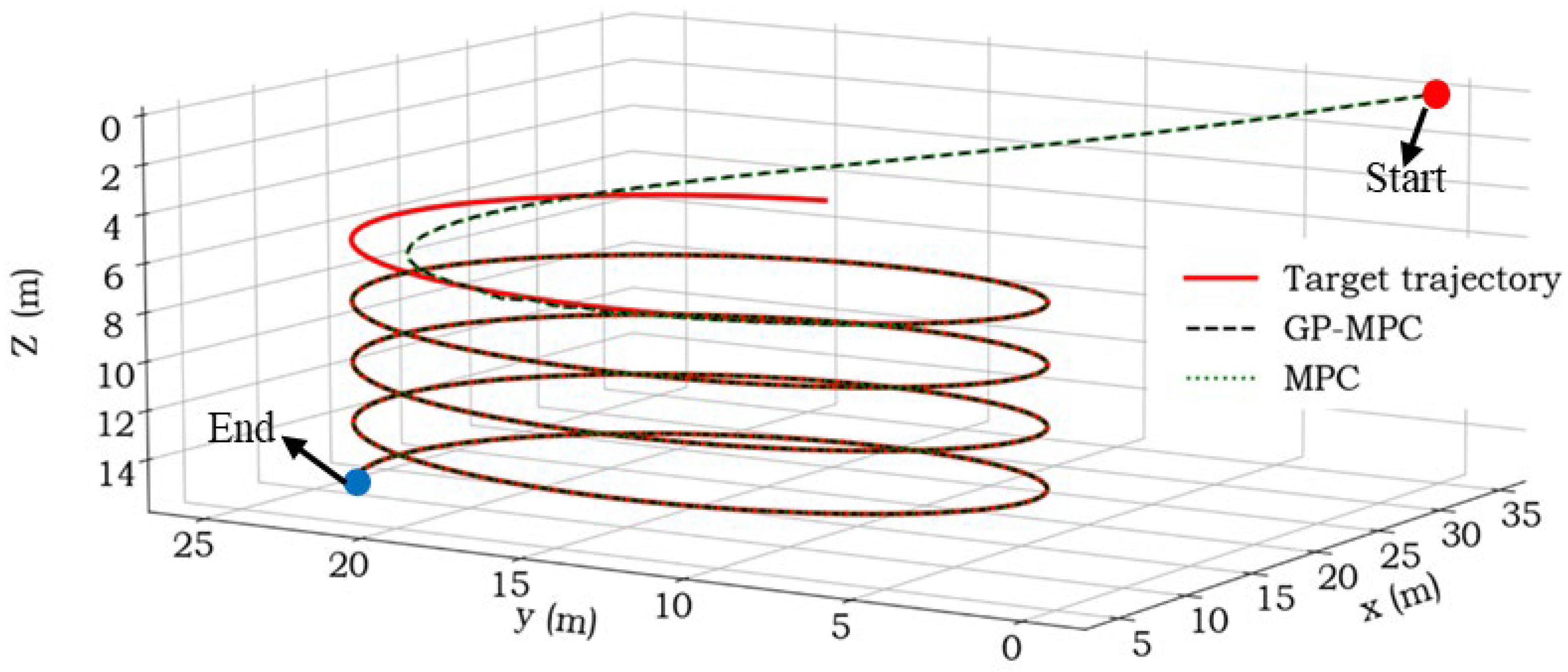
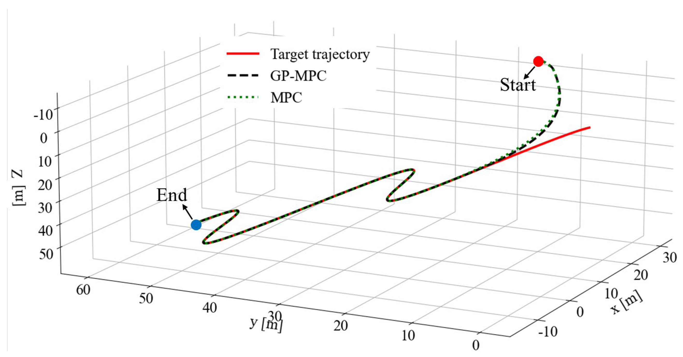
The trajectory tracking task was performed using the proposed algorithm, which leveraged available data and control inputs to guide the AUV’s motion, ensuring the precise tracking of the desired trajectory. The simulation results, depicted in Figure 3, unequivocally demonstrate the algorithm’s effectiveness in achieving accurate trajectory tracking. The red curve in Figure 3 represents the target trajectory, while the black dashed curve illustrates the actual motion trajectory of the AUV with Gaussian-process-based MPC, and the green dotted curve represents the MPC method. The remarkable alignment between these two curves demonstrates the algorithm’s ability to steer the AUV precisely along the intended path.

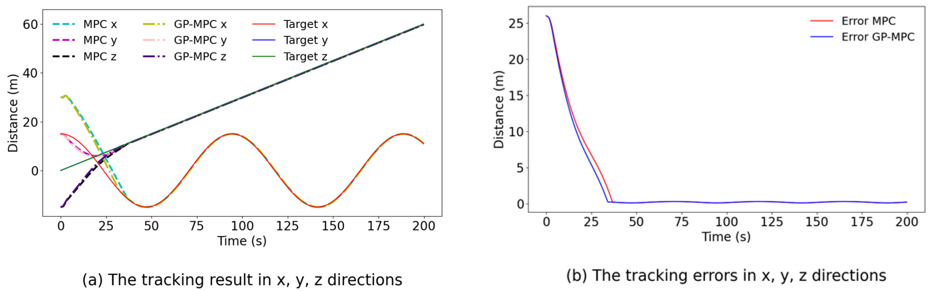
To delve deeper into the results, Figure 4 presents a comprehensive view of the tracking outcomes and errors in the $x$, $y$, and $z$ directions over time during the simulation. Figure 4a displays the target and simulated trajectories. Here, the red, blue, and green curves signify the target trajectory in the $x$, $y$, and $z$ directions, respectively. The trajectories in the $x$, $y$, and $z$ directions of Gaussian-process-based MPC trajectories are represented by the red, blue, and green curves, respectively. The yellow, pink and purple dashed curves represent the trajectories of the MPC method. From Figure 4, it is evident that the MPC and Gaussian-process-based MPC can effectively approach the target trajectory when their initial positions differ, and subsequently form a stable tracking effect. It can be observed from the approach curve during the first 20 s shown in subgraph (a) and the error curve of subgraph (b) that Gaussian-process-based MPC can approach the target curve more stably and quickly. After 20 s, the average tracking error of Gaussian-process-based MPC is $0.099\mathrm{m}$, while that of MPC is $0.227\mathrm{m}$. Overall, the results demonstrate the effectiveness and accuracy of this algorithm in maintaining good trajectory tracking performance.

The sinusoidal trajectory presents a complex and dynamic motion pattern, and this type of trajectory can be defined as follows:

$${\mathit{y}}_{\mathit{r}\mathit{e}\mathit{f}}=\left[\begin{array}{c}15\cos \frac{t}{5}\\ 0.3t\\ 0.3t\end{array}\right]$$

(58)

The initial state of the AUV is defined as ${\mathit{x}}_0={[0,0,\mathrm{0,0},\mathrm{0,0},30,15,-\mathrm{15,0},\mathrm{0,0}]}^{\mathrm{T}}$. Figure 5 and Figure 6, respectively, show the spatial trajectory tracking results and the differences in the $x$, $y,$ and $z$ components. After 50 s, the average tracking error of Gaussian-process-based MPC is $0.367 \mathrm{m}$, while that of MPC is $0.577 \mathrm{m}$. Overall, the sinusoidal trajectory tracking presents substantial challenges for the AUV due to variations in curvature and speed. Compared to the spiral curve, the tracking error of each control method increases, but can remain within a lower range after stabilization.

In summary, the algorithm has successfully demonstrated its ability to enable the AUV to meticulously track the desired trajectory, as is evident from the close alignment between the actual and desired trajectories. Furthermore, the analysis of tracking errors further confirms the algorithm’s capacity to mitigate the initial discrepancies and sustain an accurate tracking throughout the simulation. These findings highlight the algorithm’s potential to enhance trajectory control and facilitate the dependable motion of AUVs in real-world scenarios.

4.2. Avoidance of Static Obstacles on the Horizontal Plane

To validate the Gaussian-process-based MPC’s ability to handle external constraints, a series of obstacle avoidance experiments for the AUV were meticulously designed and simulated. In this comprehensive assessment of the control method’s performance, obstacles were strategically positioned within the positional space. It is important to note that, during the simulation, the AUV dynamically selects obstacles for state observation based on predefined obstacle selection rules, while disregarding others. This approach optimizes the AUV’s interactions with obstacles, enabling an in-depth study of its obstacle avoidance capabilities. The simulation encompasses gradual modifications to the size and position of the obstacles to comprehensively test the AUV’s ability to navigate around them. The selected shape for the obstacles is the conventional elliptical form, and their specific parameters are presented in

Table 2. Coordinate and scale parameters of obstacles on the horizontal plane.

Obstacles	Coordinate Parameters/(x, y)	Scale Parameter/(l, h)
Obs. 1	(17.0, 16.0)	(0.5, 1.0)
Obs. 2	(14.0, 12.0)	(0.5, 1.0)
Obs. 3	(39.0, 35.5)	(1.0, 2.0)
Obs. 4	(14.0, 12.0)	(1.0, 2.0)
Obs. 5	(25.0, 25.0)	(1.0, 2.0)

.

The first column of Table 2 denotes the obstacle number, the second column provides the Cartesian coordinates of each obstacle, and the third column specifies the size of each obstacle. The expected state for obstacle avoidance is denoted as ${\mathit{y}}_{ref}={\left[\mathrm{49,40,0}\right]}^{\mathrm{T}}$. The initial state and input values of the AUV are set as ${\mathit{x}}_0={[1.5,0,\mathrm{0,0},\mathrm{0,0}]}^{\mathrm{T}}$ and ${\mathit{u}}_0={\left[\mathrm{0,0}\right]}^{\mathrm{T}}$, respectively. Additionally, the obstacle selection parameters are set as $angle=\pi /2$ and $dir=3\mathrm{m}$. The simulation is conducted with a sampling period $T=0.1 \mathrm{s}$ and the prediction step $p=15$.

In the simulation experiments, specific constraints were imposed on the input $\mathit{u}={[T_{prop},\delta ]}^{\mathrm{T}}$ and state space $\mathit{x}={[u,v,r,x,y,\psi ]}^{\mathrm{T}}$ of the AUV to ensure safe and controlled motion. The constraints were rigorously defined as follows:

$$\begin{array}{c}{\mathit{u}}_{min}={\left[0,-\frac{30\pi }{180}\right]}^{\mathrm{T}}\\ {\mathit{u}}_{max}={\left[4.4,\frac{30\pi }{180}\right]}^{\mathrm{T}}\end{array}$$

(59a)

$$\begin{array}{c}{\mathit{x}}_{min}={\left[0,-0.9,-\frac{25\pi }{180},-INF,-INF,-INF\right]}^{\mathrm{T}}\\ {\mathit{x}}_{max}={\left[\mathrm{2,0.9},\frac{25\pi }{180},INF,INF,INF\right]}^{\mathrm{T}}\end{array}$$

(59b)

The weight matrices of the $Loss$ function are defined as follows:

$$\begin{array}{c}\mathit{Q}=\mathit{diag}\left({\mathbf{10}}^{\mathbf{-}\mathbf{6}},{\mathbf{10}}^{\mathbf{-}\mathbf{6}},{\mathbf{10}}^{-\mathbf{6}},\mathbf{10},\mathbf{10},{\mathbf{10}}^{\mathbf{-}\mathbf{1}}\right)\\ \mathit{R}=\mathrm{diag}\left({10}^{-3},{10}^{-3}\right)\\ \mathit{S}=\mathrm{diag}\left({10}^{-6},{10}^{-6}\right)\end{array}$$

(60)

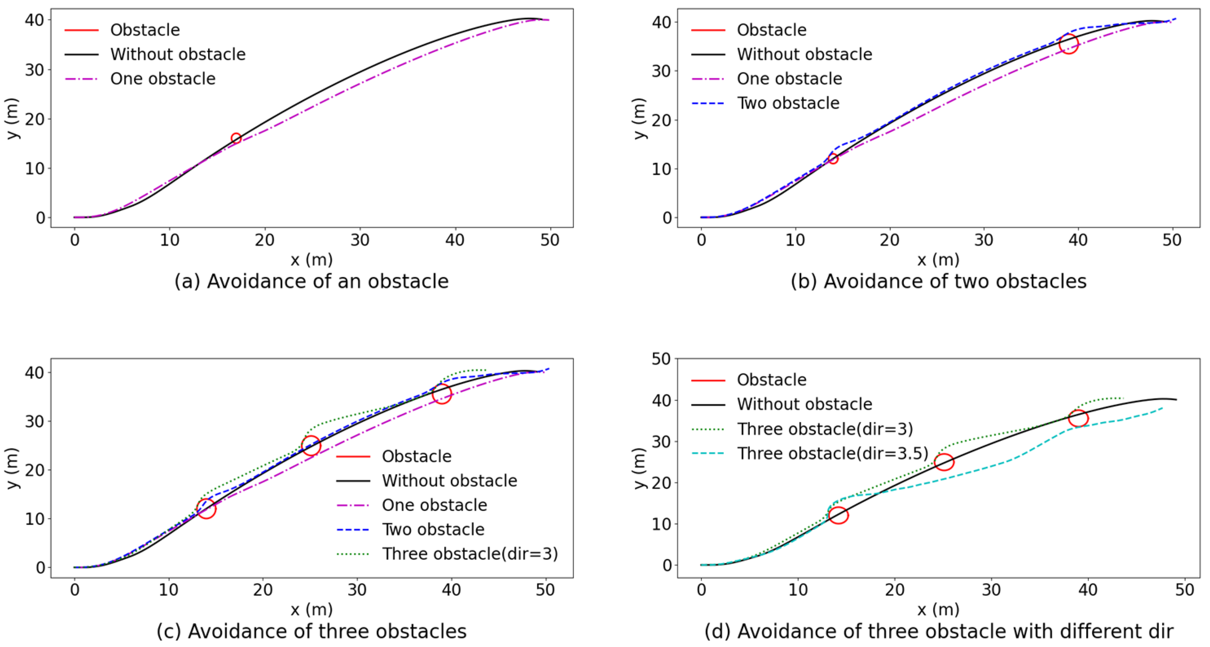
Figure 7 provides a comprehensive illustration of the simulation results, showcasing the remarkable obstacle avoidance capabilities of the AUV. The figure is thoughtfully divided into several subgraphs, with each offering unique insights into the AUV’s motion trajectories as it adeptly navigates around various obstacles. Figure 7a depicts the motion trajectory of the AUV while avoiding Obs. 1. This subgraph highlights the AUV’s ability to navigate around a single obstacle. Figure 7b illustrates the AUV’s trajectory while avoiding Obs. 2 and Obs. 3 simultaneously. The positioning of Obs. 2 at the intersection of two curves from Figure 7a allows for a rigorous evaluation of the AUV’s obstacle avoidance capabilities when encountering multiple obstacles. Figure 7c,d present the trajectories of the AUV while avoiding Obs. 3, Obs. 4, and Obs. 5. Throughout the simulation process, the parameters of the obstacles are intelligently configured based on insights gained from prior obstacle avoidance simulations. Notably, in Figure 7b, Obs. 2 is astutely positioned at the convergence point of the trajectories from Figure 7a. This deliberate arrangement is designed to challenge the AUV’s obstacle avoidance prowess by creating an environment where it encounters multiple obstacles simultaneously.

In Figure 7, the red ellipses represent the obstacles that need to be avoided, while the black curves represent the reference trajectory in the absence of obstacles. The magenta dash-dotted curves and blue dashed curves elegantly signify the AUV’s avoidance of one obstacle and two obstacles, respectively. Meanwhile, the green dotted curves and the cyan dashed curve represent the AUV’s impressive ability to avoid three obstacles, each with distinct values of $dir$. These findings are a testament to the AUV’s exceptional obstacle avoidance performance, with each subgraph showcasing its agility and precision in various challenging scenarios.

Figure 8 illustrates the translational velocities $u$ and $v$, the rotational velocity $r$, the Euler angle $\psi$, and the input $\mathit{u}={[T,\delta ]}^{\mathrm{T}}$ associated with each obstacle avoidance result. The key insights conveyed by the various curves, represented by distinct line types and colors in this figure, align with the interpretations presented in Figure 7.

From the obstacle avoidance results of the two and three obstacles presented in Figure 7b,c, and the corresponding input data displayed in Figure 8, a clear pattern emerges. During the AUV obstacle avoidance task, the effective strategy revolves around setting the rudder angle to its maximum value as the AUV approaches an obstacle. This proactive measure ensures a safe distance is maintained from the obstacle during avoidance. Once the obstacle avoidance task is successfully accomplished, the AUV smoothly transitions back towards the reference trajectory in the absence of obstacles.

Subsequently, it becomes apparent that different obstacle avoidance results can be achieved by adjusting the observation minimum distance $dir$, as illustrated in Figure 7d. When $dir$ is set to 3 m, the obstacle avoidance trajectory passes through Obs. 5 from the front. An in-depth analysis of this trajectory reveals a key behavior—the AUV endeavors to realign itself with the reference curve once it escapes the influence range of the first obstacle. This realignment is most notable between the second and third obstacles, where the AUV’s path closely aligns with the black reference trajectory. However, due to the short distance between the first and second obstacles, the AUV chooses to maintain a safe distance rather than immediately approach the reference trajectory to satisfy the obstacle avoidance requirements.

On the other hand, when $dir$ is adjusted to 3.5 m, while the AUV remains focused on the first obstacle, this extends over a more prolonged duration, allowing it to approach the reference trajectory with a lower yaw angle after successfully circumventing the obstacle. This observation is distinctly supported by Figure 8d, where the minimum value of $\psi$ is 0.1556 rad between 10 and 20 s. As the AUV shifts its focus towards the second obstacle, the controller efficiently adjusts the AUV’s trajectory based on its current state, enabling it to pass below Obs. 5 with precision. These findings serve as a testament to the versatility and adaptability of the proposed method. By strategically adjusting the observation minimum distance $dir$, the AUV can navigate complex environments with agility and ensure the safe avoidance of obstacles while maintaining trajectory accuracy.

4.3. Avoidance of Dynamic Obstacles on Horizontal Plane

While static obstacle avoidance remains a pivotal aspect of AUV control, it is imperative to recognize the equal significance of dynamic obstacle avoidance in real-world applications. In the previous sections, we delved into our approach for static obstacle avoidance. Now, we shift our focus to dynamic obstacle scenarios, building upon our prior insights. To investigate the obstacle avoidance capabilities of the proposed method in an environment containing dynamic obstacles, a new series of simulation tests has been formulated, extending from the insights gained through the previous examination of static obstacles. To further bolster the maneuverability of the AUV, an expansion was made to the range of controllable rudder angles. It is imperative to underscore that the constraints governing the state space remain unaltered, preserving the experimental setup’s consistency. However, certain adjustments were introduced to the input constraints, which are delineated as follows:

$$\begin{array}{c}{\mathit{u}}_{min}={\left[0,-\frac{35\pi }{180}\right]}^{\mathrm{T}}\\ {\mathit{u}}_{max}={[4.4,\frac{35\pi }{180}]}^{\mathrm{T}}\end{array}$$

(61)

In the context of dynamic obstacle avoidance, the obstacles selected for simulation in Section 4.2 are denoted as Obs. 3, Obs. 4, and Obs. 5. The coordinate and size parameters of these obstacles remain consistent with the previous simulations, with the introduction of velocity parameters as an additional factor, as outlined in

Table 3. Speed parameters of obstacles.

Obstacles	Speed/(u, v)
	Situation 1	Situation 2
Obs. 3	(−0.5, 0.5)	(0, −0.5)
Obs. 4	(0, 0.5)	(0, 0.5)
Obs. 5	(−0.5, 0.5)	(−0.5, 0.5)

. The incorporation of dynamic obstacles serves the purpose of simulating real-world scenarios more faithfully, where obstacles are not stationary but in motion. To simulate the movement of dynamic obstacles, a criterion is established whereby an observed obstacle initiates its motion when the distance between the AUV and the obstacle falls below a prescribed threshold, referred to as $esp$. The motion of the obstacle ceases once the AUV successfully navigates past it. By implementing this approach, a dynamic and interactive environment is created, wherein the obstacles respond dynamically to the presence and actions of the AUV. For subsequent simulation tests, the values of $esp=7\mathrm{m}$ and $dir=3.1\mathrm{m}$ are chosen as parameter settings. These values are thoughtfully chosen to establish a suitable distance threshold for initiating and terminating obstacle motion, while maintaining a safe distance during the avoidance process. The primary objective of these simulations is to evaluate the effectiveness and adaptability of the proposed method in addressing real-world scenarios where obstacles are in motion.

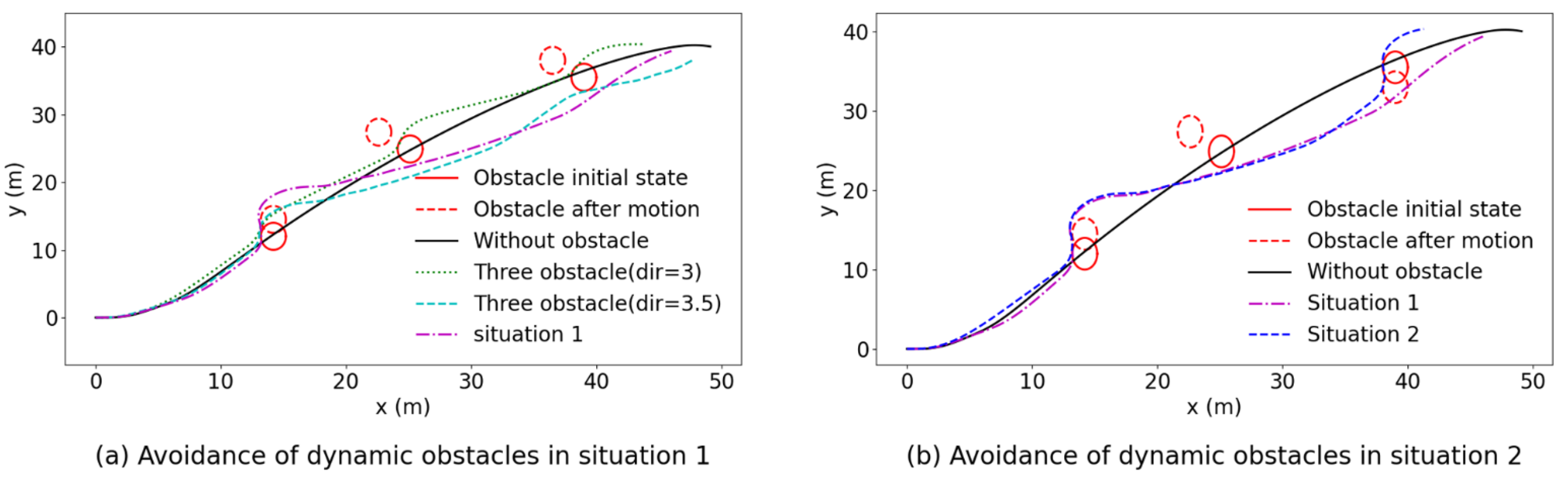
The trajectories of AUV obstacle avoidance under the influence of two types of dynamic obstacles are depicted in Figure 9. In this figure, the red solid ellipses represent the initial position of each dynamic obstacle, while the dashed ellipses denote its position after the movement has ceased. The green dotted curves and cyan dashed curve illustrate the AUV’s avoidance of the three static obstacles discussed in Section 4.2. Furthermore, the magenta dash-dotted curves and blue dashed curves represent the AUV’s avoidance trajectories when confronted with dynamic obstacles in their respective situations.

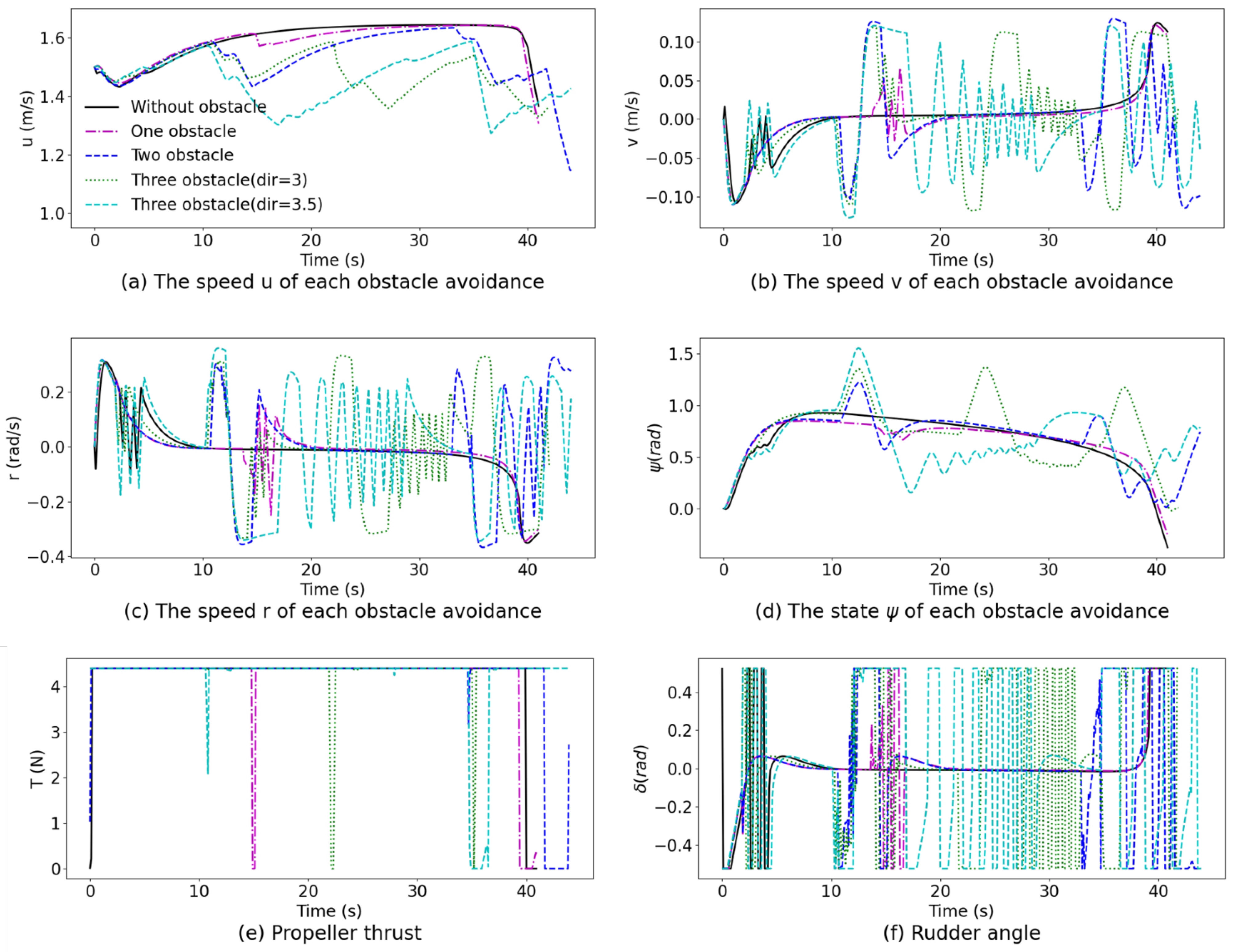
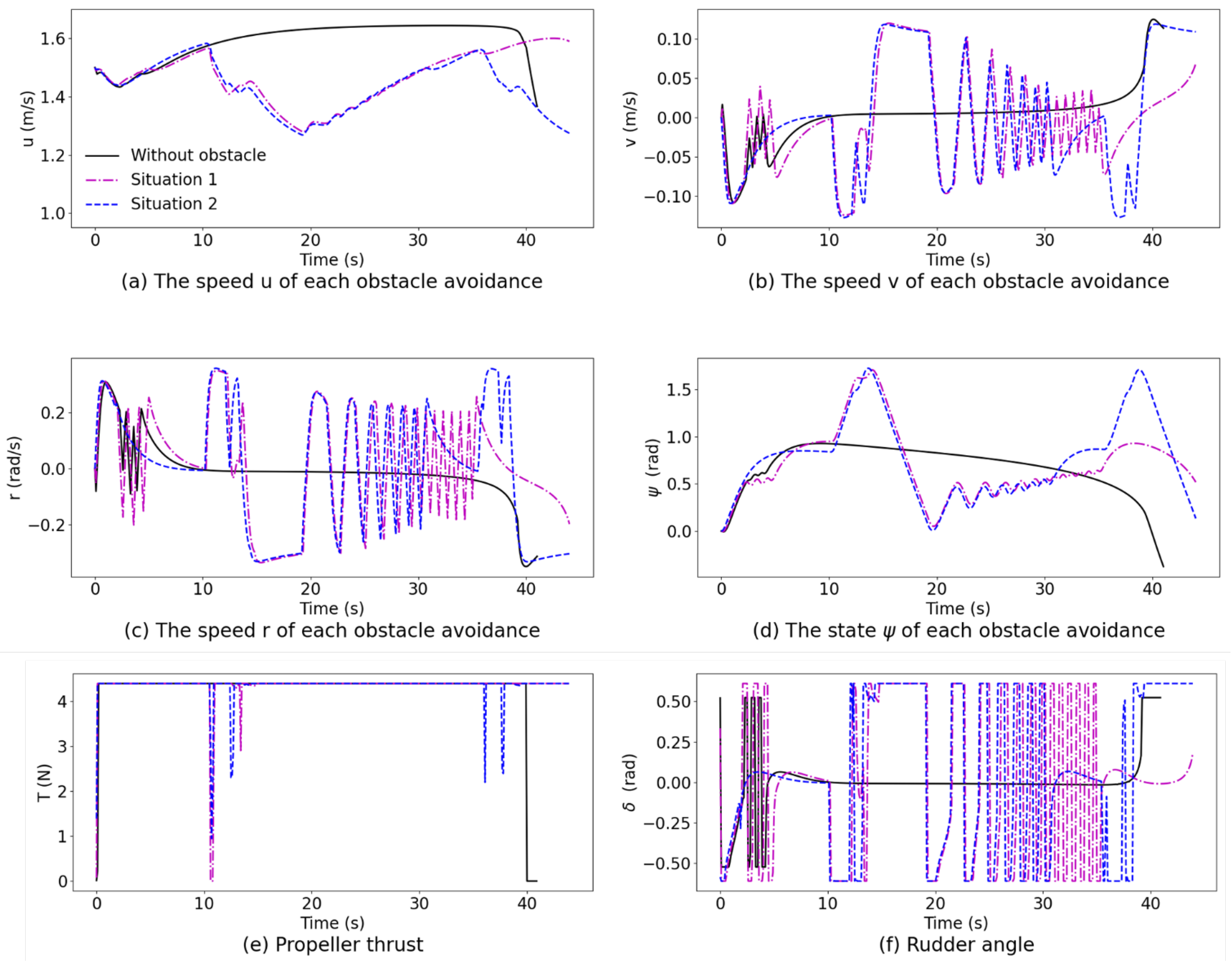
Figure 10 provides a comprehensive visualization of the translational velocities $u$ and $v$, rotational velocity $r$, Euler angle $\psi$, and input $\mathit{u}={[T,\delta ]}^{\mathrm{T}}$ for each obstacle avoidance result. An analysis of the motion trajectories in both situations reveals that the AUV follows a similar trajectory while avoiding the first two obstacles. The curves between 10 s and 30 s in each subgraph of Figure 10 demonstrate the similarities in velocity, state, and input patterns during this phase. However, a noteworthy distinction emerges in the approach adopted by the AUV when confronted with the last obstacle, which exhibits a different movement direction. This disparity is clearly evident in Figure 10d. Specifically, for situation 2, two distinct peaks of $\psi$ can be observed, measuring $1.723 \mathrm{r}\mathrm{a}\mathrm{d}$ and $1.709 \mathrm{r}\mathrm{a}\mathrm{d}$, respectively.

These simulation results highlight the adaptability of the proposed obstacle avoidance approach when dealing with dynamic obstacles. The AUV consistently performs well in avoiding the first two obstacles, with minimal deviations in trajectory, velocity, state, and input. However, the distinct movement direction of the final obstacle necessitates a unique obstacle avoidance strategy, resulting in variations in the AUV’s trajectory and ψ values. These results emphasize the effectiveness of the proposed method in dynamically navigating environments, successfully avoiding obstacles while maintaining control over the AUV’s motion.

4.4. Obstacle Avoidance in Three-Dimensional Space

Given the paramount importance of precise and secure navigation in underwater environments, particularly in mission-critical tasks such as pipeline inspection, underwater construction, and environmental monitoring, the demand for three-dimensional obstacle avoidance capabilities becomes increasingly apparent. To further enhance the obstacle avoidance capabilities of underactuated AUVs powered by fins and rudders, this section aims to extend the investigation into the effectiveness of the proposed method in the realm of three-dimensional space. Navigating obstacles in three dimensions presents distinctive challenges and offers substantial real-world applications. By expanding the scope of our research to encompass three-dimensional scenarios, valuable insights can be gained into the AUV’s ability to navigate complex underwater environments while avoiding obstacles. Furthermore, conducting research on three-dimensional obstacle avoidance is crucial for enhancing the safety and operational efficiency of autonomous underwater systems. Numerous critical underwater missions require precise and reliable navigation in three-dimensional space, such as the inspection of pipelines, underwater construction endeavors, and rigorous environmental monitoring. By enabling AUVs to autonomously navigate and avoid obstacles in three dimensions, the proposed method has the potential to significantly improve the success and accuracy of such missions, while concurrently curtailing the risk of collisions or harm to delicate underwater structures.

In this study, we delve into the realm of three-dimensional space to scrutinize the efficacy of obstacle avoidance using an underactuated AUV outfitted with both fins ${\delta }_s$ and rudders ${\delta }_r$, and the input becomes $\mathit{u}={[T_{prop},{\delta }_r,{\delta }_s]}^{\mathrm{T}}$. The target coordinates to be reached are set as $goal={\left[\mathrm{49,40,40}\right]}^{\mathrm{T}}$. The AUV’s initial speed is prescribed as 1.5 m/s, and the input is initialized as ${\mathit{u}}_0={[\mathrm{0,0},0]}^{\mathrm{T}}$. The sampling period is set as $T=0.2 \mathrm{s}$, and a prediction step of $p=10$ is employed to forecast the AUV’s forthcoming trajectory. The coordinate and scale parameters of obstacles are shown in

Table 4. Coordinate and scale parameters of obstacles in 3D space.

	Figure 8a (Position), (Scale)	Figure 8b (Position), (Scale)	Figure 8c (Position), (Scale)	Figure 8d (Position), (Scale)
Obs. 1	(14, 9.5, 13.5) (1.1, 1, 1)	(14, 9.5, 9) (0.5, 1, 1)	(8.5, 5, 5) (1, 1, 1)	(8.5, 5, 5) (1, 1, 1)
Obs. 2	(39, 35, 35) (1, 2, 2)	(39, 31, 35) (1, 2, 2)	(43, 38, 38) (1, 2, 2)	(43, 38, 36) (1, 2, 2)
Obs. 3	(25, 22, 22) (2, 2, 3)	(25, 22, 22) (2, 2, 3)	(32, 26, 32) (2, 2, 2)	(32, 26, 28) (2, 2, 2)
Obs. 4	\ \	\ \	(20, 12.5, 18) (2, 2, 2)	(20, 15, 17) (2, 2, 3)

. The first ternary array represents the coordinate of the obstacles in the spatial coordinate system, while the second array represents the scale in the $x$, $y$, and $z$ directions. In order to guarantee the effectiveness and safety of the AUV’s motion, the input constraints are modified as follows:

$$\begin{array}{c}{\mathit{u}}_{min}={\left[0,-\frac{35\pi }{180},-\frac{30\pi }{180}\right]}^{\mathrm{T}}\\ {\mathit{u}}_{max}={[4.4,\frac{35\pi }{180},\frac{30\pi }{180}]}^{\mathrm{T}}\end{array}$$

(62)

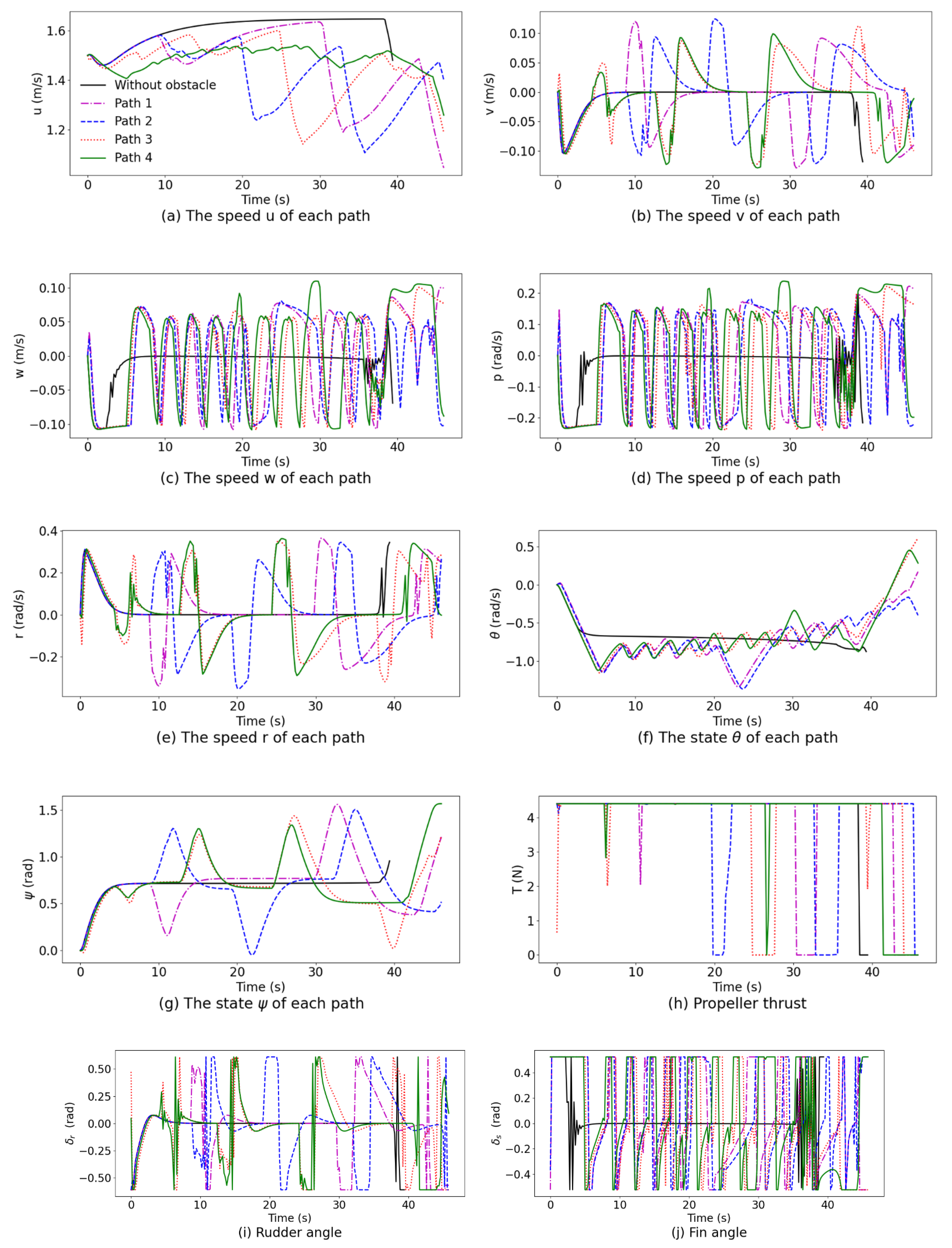
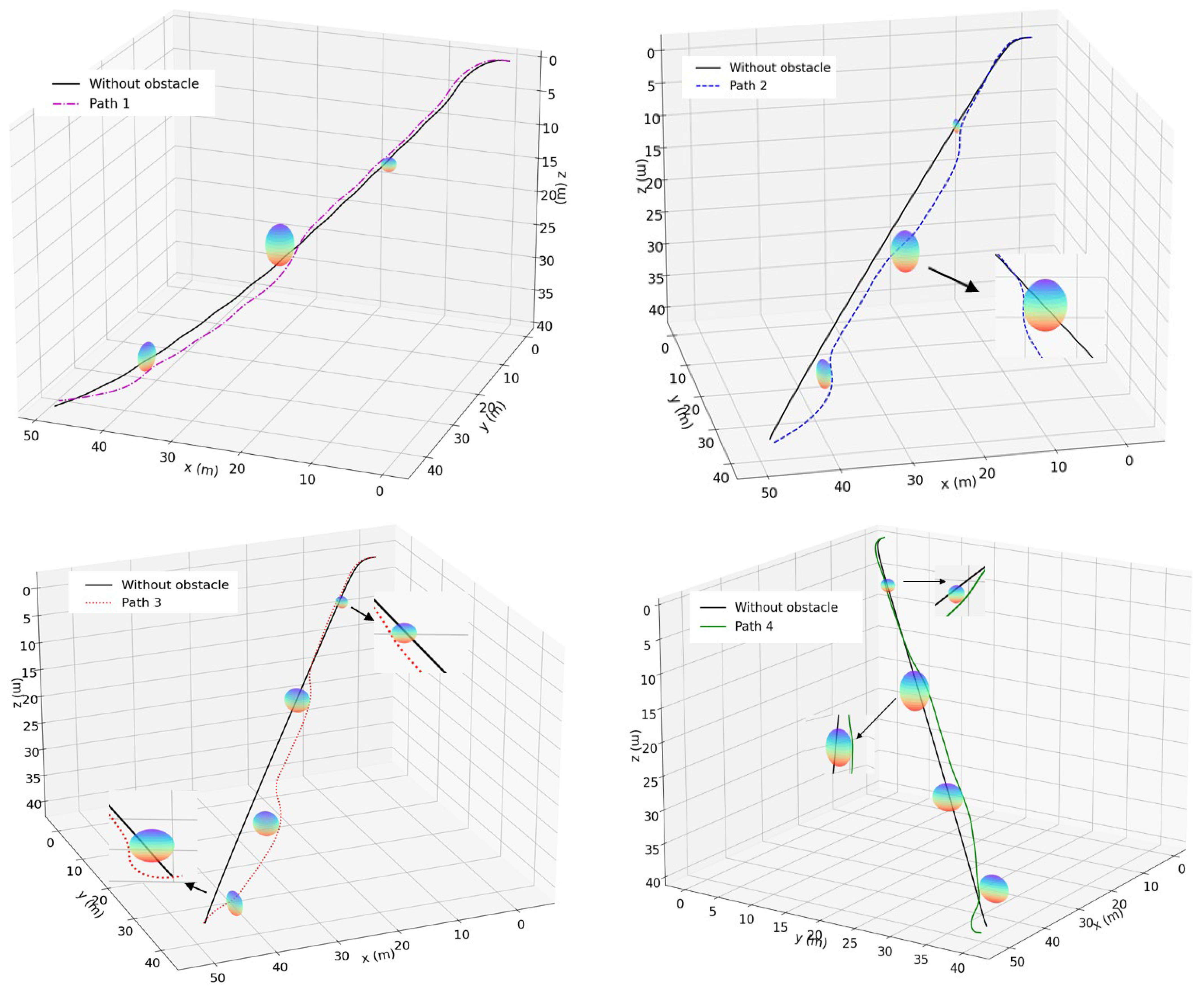
The efficacy of the proposed method in achieving three-dimensional obstacle avoidance for the AUV is substantiated by the results illustrated in Figure 11 and Figure 12. In Figure 11, the AUV obstacle avoidance paths are depicted for four distinct scenarios. The black solid line represents the path without any obstacles, while the magenta dash-dotted curve, blue dashed curve, red dotted curve, and greed curve represent the AUV’s obstacle avoidance trajectories in their respective scenarios. Correspondingly, Figure 12 provides insight into the AUV’s state and input under these four scenarios, maintaining the same representation as in Figure 11. Analyzing the simulation results, it is evident that the proposed method remarkably enables the AUV to adeptly navigate three-dimensional space while avoiding obstacles. Additionally, the AUV’s state variables and input parameters consistently adhere to the specified constraint range throughout the obstacle avoidance maneuvers. It is essential to note that, owing to the disparity between the center of gravity and center of buoyancy in the $z_b$ direction, maintaining the AUV’s stability during movement necessitates significant adjustments in the fin angle during the control process.

The results from these simulations validate the efficacy of the proposed method in enabling three-dimensional obstacle avoidance for the AUVs. The AUV adeptly maneuvers around obstacles while strictly adhering to the constraints governing its state and input. This research serves as a valuable contribution to the field of autonomous underwater systems, shedding light on effective three-dimensional obstacle avoidance strategies and elevating the overall competency and safety of AUVs operating in intricate underwater environments.

5. Conclusions

This study presents a comprehensive exploration of the control performance of the Gaussian-process-based model predictive control (GP-MPC) technique concerning trajectory tracking and obstacle avoidance in AUVs. The research commences with the establishment of the kinematic and dynamic equations governing AUV motion, providing a fundamental framework for subsequent developments. The state prediction equation, incorporating the GP-MPC methodology, is then formulated, accounting for both self-constraints and obstacle avoidance considerations while integrating an optimization function. Extensive simulations are conducted to comprehensively evaluate the performance of the proposed approach in terms of trajectory tracking and static as well as dynamic obstacle avoidance. The results validate the efficacy of the GP-MPC method in facilitating AUVs to navigate adeptly within their own constraints and effectively circumvent external obstacles. This facilitates precise and efficient obstacle avoidance control, which is crucial for ensuring AUV safety and mission success in complex underwater environments. Moreover, the study extends to the exploration of three-dimensional obstacle avoidance, providing valuable insights into the algorithm’s resilience and performance within intricate underwater environments. The research outcomes not only contribute significantly to advancing AUV capabilities and safety, but also hold substantial potential for the evolution of autonomous underwater systems. Future research endeavors may concentrate on further refining the algorithm and delving into its practical applications, with the aim of enhancing the overall dependability and efficacy of AUV obstacle avoidance strategies in real-world scenarios.

In future research, the in-depth integration of Gaussian Process Model Predictive Control (GP-MPC) with other advanced artificial intelligence techniques will become an important exploration direction, aiming to significantly enhance the intelligence level and overall performance of control systems. Such integration will not only help strengthen the adaptability and robustness of the system but also improve the accuracy and efficiency of decision-making. In addition, it is crucial to investigate how to better handle multi-objective optimization problems and constraints using the GP-MPC method. In practical applications, control systems often need to make decisions while satisfying multiple objectives and constraints, posing higher demands on optimization algorithms. Therefore, we need to delve deeper into multi-objective optimization theory, explore effective constraint handling methods, and integrate them with the GP-MPC algorithm to achieve a more intelligent and efficient control system design.

References

1. Hong, L.; Fang, R.; Cai, X.; Wang, X. Numerical investigation on hydrodynamic performance of a portable AUV. J. Mar. Sci. Eng. 2021, 9, 812. [Google Scholar] [CrossRef]
2. Zhang, F.; Marani, G.; Smith, R.N.; Choi, H.T. Future trends in marine robotics [TC Spotlight]. IEEE Robot. Autom. Mag. 2015, 22, 14–122. [Google Scholar] [CrossRef]
3. Sagala, F.; Bambang, R.T. Development of sea glider autonomous underwater vehicle platform for marine exploration and monitoring. Indian J. Geo-Mar. Sci. 2011, 40, 287–295. [Google Scholar]
4. Wang, H.; Su, B. Event-triggered formation control of AUVs with fixed-time RBF disturbance observer. Appl. Ocean. Res. 2021, 112, 102638. [Google Scholar] [CrossRef]
5. Cong, Z.; Ma, T.; Li, Y.; Yuan, M.; Ling, Y.; Du, H.; Qi, C.; Li, Z.; Xu, S.; Zhang, Q. A Storage-Saving Quadtree-Based Multibeam Bathymetry Map Representation Method. J. Mar. Sci. Eng. 2023, 11, 709. [Google Scholar] [CrossRef]
6. Tang, Y.; Wang, L.; Jin, S.; Zhao, J.; Huang, C.; Yu, Y. AUV-Based Side-Scan Sonar Real-Time Method for Underwater-Target Detection. J. Mar. Sci. Eng. 2023, 11, 690. [Google Scholar] [CrossRef]
7. Kirkwood, W.J. Development of the DORADO mapping vehicle for multibeam, subbottom, and sidescan science missions. J. Field Robot. 2007, 24, 487–495. [Google Scholar] [CrossRef]
8. Thomas, C.; Simetti, E.; Casalino, G. A unifying task priority approach for autonomous underwater vehicles integrating homing and docking maneuvers. J. Mar. Sci. Eng. 2021, 9, 162. [Google Scholar] [CrossRef]
9. Curtin, T.B.; Crimmins, D.M.; Curcio, J.; Benjamin, M.; Roper, C. Autonomous underwater vehicles: Trends and transformations. Mar. Technol. Soc. J. 2005, 39, 65–75. [Google Scholar] [CrossRef]
10. Xia, Y.; Xu, K.; Huang, Z.; Wang, W.; Xu, G.; Li, Y. Adaptive energy-efficient tracking control of a X rudder AUV with actuator dynamics and rolling restriction. Appl. Ocean. Res. 2022, 118, 102994. [Google Scholar] [CrossRef]
11. Gong, P.; Yan, Z.; Zhang, W.; Tang, J. Trajectory tracking control for autonomous underwater vehicles based on dual closed-loop of MPC with uncertain dynamics. Ocean. Eng. 2022, 265, 112697. [Google Scholar] [CrossRef]
12. Wang, H.; Chen, B.; Lin, C. Direct adaptive neural tracking control for a class of stochastic pure-feedback nonlinear systems with unknown dead-zone. Int. J. Adapt. Control. Signal Process. 2013, 27, 302–322. [Google Scholar] [CrossRef]
13. Zhang, Y.; Liu, X.; Luo, M.; Yang, C. MPC-based 3-D trajectory tracking for an autonomous underwater vehicle with constraints in complex ocean environments. Ocean. Eng. 2019, 189, 106309. [Google Scholar] [CrossRef]
14. Khodayari, M.H.; Balochian, S. Modeling and control of autonomous underwater vehicle (AUV) in heading and depth attitude via self-adaptive fuzzy PID controller. J. Mar. Sci. Technol. 2015, 20, 559–578. [Google Scholar] [CrossRef]
15. Qiao, L.; Yi, B.; Wu, D.; Zhang, W. Design of three exponentially convergent robust controllers for the trajectory tracking of autonomous underwater vehicles. Ocean. Eng. 2017, 134, 157–172. [Google Scholar] [CrossRef]
16. Peng, Z.; Wang, J.; Wang, J. Constrained control of autonomous underwater vehicles based on command optimization and disturbance estimation. IEEE Trans. Ind. Electron. 2018, 66, 3627–3635. [Google Scholar] [CrossRef]
17. Cho, Y.; Han, J.; Kim, J.; Lee, P.; Park, S.B. Experimental validation of a velocity obstacle based collision avoidance algorithm for unmanned surface vehicles. IFAC-PapersOnLine 2019, 52, 329–334. [Google Scholar] [CrossRef]
18. Trym, T.; Brekke, E.F.; Johansen, T.A. On collision risk assessment for autonomous ships using scenario-based MPC. IFAC-PapersOnLine 2020, 53, 14509–14516. [Google Scholar] [CrossRef]
19. Zhang, M.; Hao, S.; Wu, D.; Chen, M.L.; Yuan, Z.M. Time-optimal obstacle avoidance of autonomous ship based on nonlinear model predictive control. Ocean. Eng. 2022, 266, 112591. [Google Scholar] [CrossRef]
20. Bao, H.; Zhu, H.; Li, X.; Liu, J. APSO-MPC and NTSMC Cascade Control of Fully-Actuated Autonomous Underwater Vehicle Trajectory Tracking Based on RBF-NN Compensator. J. Mar. Sci. Eng. 2022, 10, 1867. [Google Scholar] [CrossRef]
21. Oh, S.R.; Sun, J. Path following of underactuated marine surface vessels using line-of-sight based model predictive control. Ocean. Eng. 2010, 37, 289–295. [Google Scholar] [CrossRef]
22. Gao, J.; Liu, C.; Proctor, A. Nonlinear model predictive dynamic positioning control of an underwater vehicle with an onboard USBL system. J. Mar. Sci. Technol. 2016, 21, 57–69. [Google Scholar] [CrossRef]
23. Wang, W.; Yan, J.; Wang, H.; Ge, H.; Zhu, Z.; Yang, G. Adaptive MPC trajectory tracking for AUV based on Laguerre function. Ocean. Eng. 2022, 261, 111870. [Google Scholar] [CrossRef]
24. Song, Y.; Scaramuzza, D. Policy search for model predictive control with application to agile drone flight. IEEE Trans. Robot. 2022, 38, 2114–2130. [Google Scholar] [CrossRef]
25. Piotr, B.; Zwierzewicz, Z. Ship course-keeping algorithm based on knowledge base. Intell. Autom. Soft Comput. 2011, 17, 149–163. [Google Scholar]
26. Yao, F.; Yang, C.; Liu, X.; Zhang, M. Experimental evaluation on depth control using improved model predictive control for autonomous underwater vehicle (AUVs). Sensors 2018, 18, 2321. [Google Scholar] [CrossRef]
27. Uchihori, H.; Cavanini, L.; Tasaki, M.; Majecki, P.; Yashiro, Y.; Grimble, M.J.; Yamamoto, I.; van der Molen, G.M.; Morinaga, A.; Eguchi, K. Linear parameter-varying model predictive control of AUV for docking scenarios. Appl. Sci. 2021, 11, 4368. [Google Scholar] [CrossRef]
28. Maciejowski, J.M.; Yang, X. Fault tolerant control using Gaussian processes and model predictive control. In Proceedings of the 2013 Conference on Control and Fault-Tolerant Systems (SysTol), Nice, France, 9–11 October 2013; IEEE: Piscataway, NJ, USA, 2013; pp. 1–12. [Google Scholar]
29. Hewing, L.; Liniger, A.; Zeilinger, M.N. Cautious NMPC with Gaussian process dynamics for autonomous miniature race cars. In Proceedings of the 2018 European Control Conference (ECC), Limassol, Cyprus, 12–15 June 2018; IEEE: Piscataway, NJ, USA, 2018; pp. 1341–1348. [Google Scholar]
30. Li, D.; Du, L. Auv trajectory tracking models and control strategies: A review. J. Mar. Sci. Eng. 2021, 9, 1020. [Google Scholar] [CrossRef]
31. Mehdi Khosrow-Pour, D.B.A. Advances in Information Quality and Management. In Encyclopedia of Information Science and Technology, 5th ed.; IGI Global: Hershey, PA, USA, 2020; Volume 1, Chapter 1; pp. 1–11. [Google Scholar]
32. Do, K.D.; Pan, J. Control of Ships and Underwater Vehicles: Design for Underactuated and Nonlinear Marine Systems; Springer: London, UK, 2009. [Google Scholar]
33. Fossen, T.I. Handbook of Marine Craft Hydrodynamics and Motion Control; John Wiley & Sons: Hoboken, NJ, USA, 2011. [Google Scholar]
34. Prestero, T.T.J. Verification of a Six-Degree of Freedom Simulation Model for the REMUS Autonomous Underwater Vehicle. Ph.D. Thesis, Massachusetts Institute of Technology, Cambridge, MA, USA, 2001. [Google Scholar]
Figure 1. Coordinate system of AUV in six degrees of freedom.
Jmse 12 00676 g001
Figure 2. The framework of GP-MPC.
Jmse 12 00676 g002
Figure 3. The results of spiral trajectory tracking.
Jmse 12 00676 g003
Figure 4. The tracking results and errors with time during simulation for tracking spiral trajectory.
Jmse 12 00676 g004
Figure 5. The results of sinusoidal trajectory tracking.
Jmse 12 00676 g005
Figure 6. The tracking results and errors with time during simulation for tracking sinusoidal trajectory.
Jmse 12 00676 g006
Figure 7. Horizontal static obstacle avoidance.
Jmse 12 00676 g007
Figure 8. The translational velocity u , v , rotational velocity r , Euler angle ψ , and input u = [ T , δ ] T of each static obstacle avoidance result.
Jmse 12 00676 g008
Figure 9. Horizontal dynamic obstacle avoidance.
Jmse 12 00676 g009
Figure 10. The translational velocity u , v , rotational velocity r , Euler angle ψ , and input u = [ T , δ ] T for each dynamic obstacle avoidance result.
Jmse 12 00676 g010
Figure 11. Obstacle avoidance in 3D space.
Jmse 12 00676 g011
Figure 12. The state and input for each obstacle avoidance path.
Jmse 12 00676 g012