Anti-Eavesdropping by Exploiting the Space–Time Coupling in UANs

Abstract

Due to the space–time coupling access, we find that anti-eavesdropping opportunities exist in underwater acoustic networks (UANs), where packets can be successfully received only by the intended receiver, but collide at the unintended receivers. These opportunities are highly spatially dependent, and this paper studies the case that linearly deployed sensor nodes directly report data toward a single collector. We found an eavesdropping ring centered around these linearly deployed sensor nodes, where the eavesdropper could steal all the reported data. Since the typical receiving-alignment-based scheduling MAC (TRAS-MAC) will expose the relative spatial information among the sensor nodes with the collector, the eavesdropper can locate the eavesdropping ring. Although moving the collector into the one-dimensional sensor node chain can degrade the eavesdropping ring to a point that constrains the eavesdropping risk, the collector’s location will be subsequently exposed to the eavesdropper. To efficiently protect the reported data and prevent the exposure of the collector’s location, we designed a slotted- and receiving-alignment-based scheduling MAC (SRAS-MAC). The NS-3 simulation results showed the effectiveness of the SRAS-MAC and the TRAS-MAC in protecting data from eavesdropping, which protect 90% of the data from eavesdropping in the one-eavesdropper case and up to 80% of data from eavesdropping in ten-eavesdropper cases. Moreover, unlike TRAS-MAC, which will expose the collector’s location, SRAS-MAC provides multiple positions for the collector to hide, and the eavesdropper cannot distinguish where it is.

1. Introduction

Underwater acoustic sensor networks (UASNs) have been deployed to acquire various data of interest beneath the water surface for decades [1,2]. In recent years, data-driven approaches have been widely adopted in acoustic channel estimation, geoacoustic inversion, and so on, causing a geometric growth in the underwater data volume [3,4]. This fact requires the advancement of an efficient and secure medium access control (MAC) mechanism to collect the data from the UASNs.

The current efforts on the MAC design in underwater acoustic networks (UANs) are mainly focused on improving access efficiency from the perspective of time division, since the narrow available bandwidth and the harsh underwater acoustic channel limit the use of frequency division and code division [5,6]. The challenge is basically attributed to the non-negligible propagation delay caused by the relatively slow propagation speed, which is about 1500 m/s and five orders slower than the radio wave propagated through the air [7]. This results in space–time coupling access in UANs and makes the MAC more complicated than in terrestrial radio networks (TRNs) [8,9]. On the one hand, since the spatial distance from its sender to its receiver jointly decides the packet’s arrival time, solely separating the sending times at the sending sides cannot guarantee their packets are collision-free at the receiving sides. On the other hand, the extra spatial factor provides more opportunities to align designated packets and aggregate interference (The other arriving packets.) at each node [10]. It has been proven that the upper-bound of normalized throughput for mesh-connected UANs is $\frac{N}{2}$, which is greater than can be achieved in TRNs [11]. For the star-connected UANs, allocating the sending times of senders according to their spatial distances to the common receiver to achieve perfect receiving-alignment in the receiver can reach the upper-bound of normalized throughput, which is alwaysone [8].

Two techniques have been used to promote data confidentiality in UANs, including encryption and physical layer security (PLS) [12]. Encryption uses a secret key to encrypt the message before data dissemination. The idea of the PLS approach is to utilize the random nature of wireless channels to promote the secrecy rate between legal users. Unfortunately, the cost and challenge are heavier for implementing encryption and the PLS in UANs than in TRNs. First, a portion of limited bandwidth is taken for regular updates of the secret key, not for data transmission [13,14]. Second, the security rate of the PLS approach is directly related to the estimation accuracy on the dynamic multi-path acoustic channel and underwater noise [15,16]. As it stands currently, both of these methods are decoupled from the MAC layer in UANs.

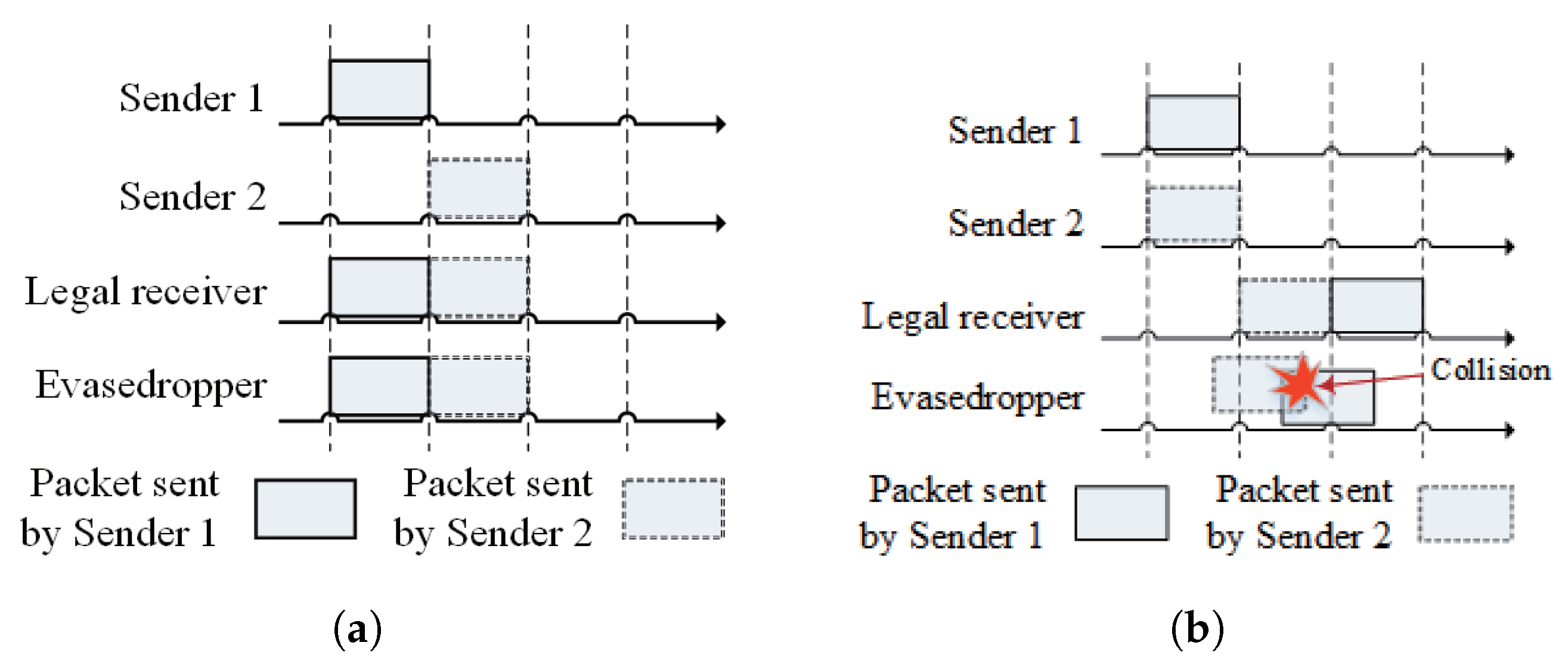
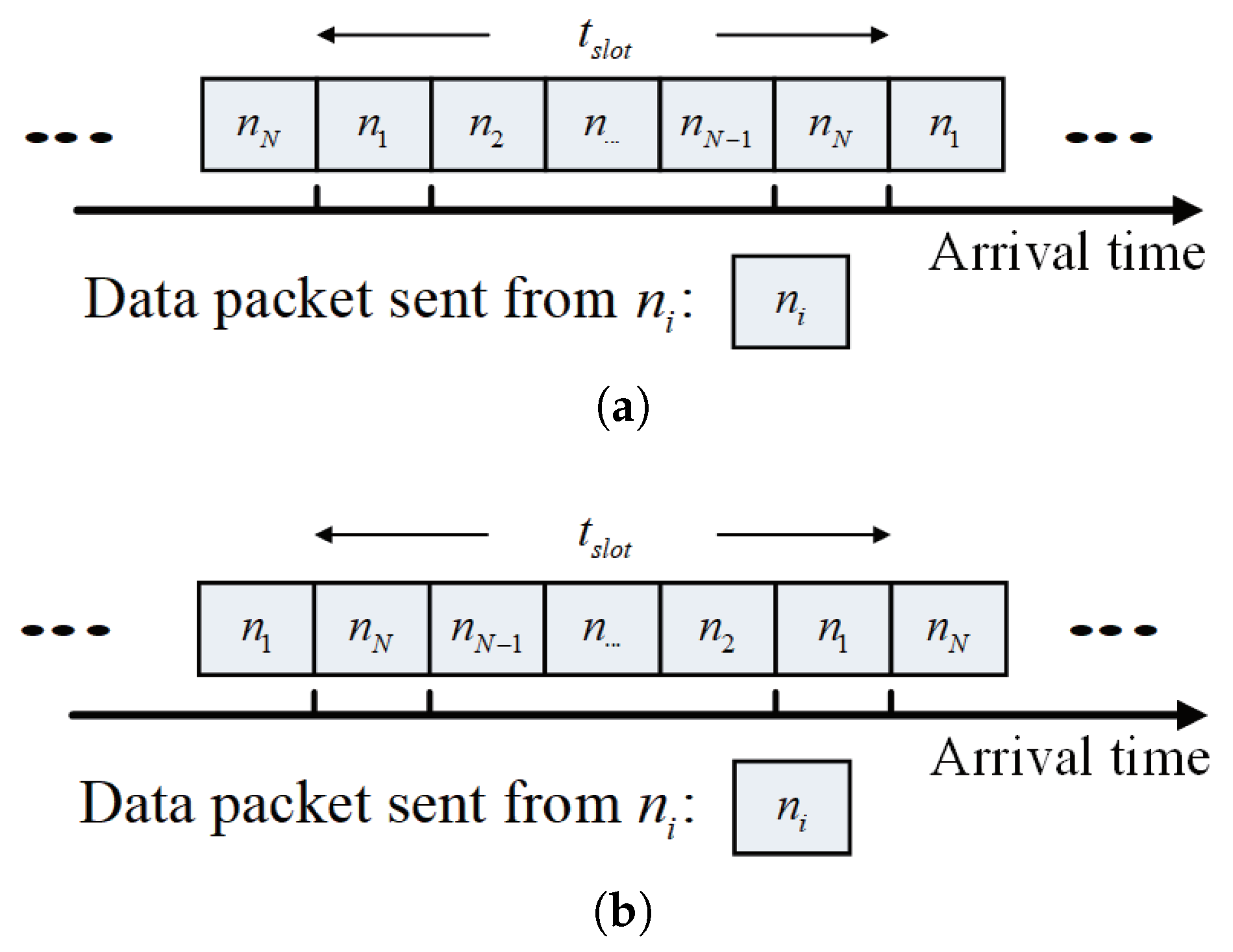
Owing to the open nature of wireless communication, a wireless signal can be overheard by all the nodes within the coverage of its sender. Since the arrival time is only determined by the sending time in TRNs, as shown in Figure 1a, the collision-free multiple access to the intended receiver also means collision-free multiple access to any other unintended nodes within the coverage of the senders. On the contrary, due to the space–time coupling characteristic, the well-scheduled sending times toward the intended receiver are unlikely to match with the relative distances toward the unintended receiver. As illustrated in Figure 1b, the packets can only be successfully received by the legal receiver and collide at the eavesdropper. Therefore, the space–time coupling characteristics of UANs naturally have opportunities for anti-eavesdropping. In this sense, it is recommended to integrate a receiving-aggregation design that creates heavy packet collisions at unintended receivers while ensuring collision-free access for intended receivers in UANs.

Actually, the adversary receiver is also incentivized to exploit the space–time coupling access to maximize the number of packets it can successfully receive without collision. A MAC protocol without anti-eavesdropping concerns might create some areas where numerous or even all the packets can be successfully received without collision. The eavesdropper is eager to acquire the spatial information and the legal nodes’ sending times to find such eavesdropping areas to facilitate its eavesdropping performance. Therefore, it is required to carefully design the MAC protocol and expose as little spatial information as possible.

This paper aims to exploit the space–time coupling characteristic to achieve both efficient and secure MAC while a group of linearly deployed underwater sensor nodes report their data to a single collector. The linear and grid topology constructed by multiple linear node chains are the most-common patterns and are widely applied in UANs [17,18,19]. As a result, the network performance of linearly deployed UANs still attracts the interest of some researchers.

The contributions of this paper are summarized as follows:

• Anti-eavesdropping opportunities of space–time coupling access: The anti-eavesdropping opportunity and the rest of the risk of being eavesdropped in the MAC layer of UANs are first discussed in this paper. This anti-eavesdropping capability is achieved by causing continuous packet collisions on unintended receivers through MAC layer design. As a result, there are no additional hardware requirements compared to the existing MAC in UANs. It is expected to encourage the study of integrating and promoting the anti-eavesdropping ability while achieving efficient MAC in UANs.
• Eavesdropping from linearly deployed sensor nodes: For a star-connected network formed by a group of linearly deployed sensor nodes and a single receiver, we find an eavesdropping ring centered around the node chains, where all the packets sent by the sensor nodes can be successfully received. The typical receiving-alignment-based MAC (TRAS-MAC) needs to allocate and notice the sending time of each sensor node one by one. In this case, the spatial information, i.e., relative distances among sensor nodes to the receiver, can be easily acquired by the adversary eavesdropper. If the eavesdropper acquires the positions of these anchored sensor nodes, the eavesdropper can locate the eavesdropping ring and steal all the packets. The anti-eavesdropping can be shrunk into a single point when the legal receiver is also located inside the same one-dimensional space where sensor nodes are located, which essentially limits the possibility of perfect eavesdropping. Moreover, we prove that assigning the distance-dependent arrival order of packets at the legal receiver, i.e., closer distance, earlier arrival and farther distance, earlier arrival, perform better in anti-eavesdropping than using random order. We also find that an even number of sensor nodes causes more collision in the eavesdropper than an odd number of sensor nodes while using a distance-dependent arrival order of packets.
• Anti-eavesdropping MAC design: Since the spatial information is still exposed to the eavesdropper and can precisely locate the legal receiver in the one-dimensional space, the TRAS-MAC must be improved. We propose a slotted- and receiving-alignment-based MAC protocol (SRAS-MAC) to achieve safe and efficient medium access from linearly deployed sensor nodes to a single receiver. The SRAS-MAC chose a proper packet size according to the network information, e.g., spacing distance between two neighboring sensor nodes, amount of sensor nodes, and so on, to achieve perfect receiving-alignment and attain maximal capacity. Since the sending time remains the same and periodic among all sensor nodes, the eavesdropper cannot deduce spatial information from it. Furthermore, the SRAS-MAC provides a group of optional locations for the legal receiver, each of which can achieve similar network and anti-eavesdropping performance. Therefore, the proposed SRAS-MAC can also protect the location privacy of the legal receiver since the adversary eavesdropper cannot distinguish where the legal receiver is located.

Related Work

Work can be found in understanding the space–time coupling characteristic, but it solely focuses on decreasing interference and prompting normalized throughput in the MAC layer.

In distributed MAC design, a protection interval is always used to eliminate the spatial impact during the medium access in UANs [5]. However, this inevitably causes long waiting or decreased access opportunities, while floor acquisition or random access are used, respectively [20,21,22,23,24].

Our work relates more to a scheduling-based MAC protocol, which takes advantage of the long propagation delay to promote the network throughput [8,10,11,25,26,27]. The upper-bound about the throughput of N-node Ad Hoc UANs in the MAC layer have been proven to be $\frac{N}{2}$ by Chitre et al., which is greater than the N-node Ad Hoc TRNs [11]. An efficient approach to solve the scheduling problem is formulating it into an optimization problem with the goal of maximizing throughput, where the sending times and packet duration are the optimal solutions to this problem [10]. However, the Computational complexity increases as the number of nodes grows. On the other hand, the upper-bound for the throughput on star-connected networks remains at one regardless of the number of senders. This can be achievable by the receiving-alignment-based MAC proposed by Chen et al., which assigns the sending times of each sender one by one based on the spatial information and the arrival order of the packets in the receiver [8]. Wang et al. proved that spatial reuse can be achieved while using the slotting technique in the star-connected network as long as the slot length is greater than two-times the packet duration, which helps to understand further the impact of space–time coupling on the slotted-based MAC in UANs [9].

Our work is also related to the medium access control among multiple linearly deployed sensor nodes. Current research mainly focuses on solving this by using hop by hop relaying and the throughput under different considerations, e.g., partially overlapping collision domain with single traffic flow and single collision domain with unicast traffic, which have been discussed by Bai et al. and Said et al., respectively. However, relaying faces a series of challenges, such as complex interference, unbalanced traffic load, hot zones in energy consumption, and so on. Although Chen et al. have shown that multi-hop forwarding faces less energy consumption compared to direct access due to less path loss [28], the adopted frequencies for both direct access and multi-hop forwarding are 100kHz, which limits the discussion in a small-scale network. Actually, whether single-hop or multi-hop transmission performs better in a linear network is still an open question in wireless networks. Sikora et al. revealed that single-hop communication is more suitable for the bandwidth-limited scenario compared to multi-hop communication in an equidistantly deployed linear wireless network [29]. Li et al. found that direct access is more energy efficient if the transmission distance is less than an open distance in UANs [30]. Using direct access, these linearly deployed sensor nodes and the collector construct a star-connected network.

The remainder of this paper is arranged as follows. Section 2 describes the system we studied. The security risks in the linearly deployed and star-connected network are discussed in Section 3. In Section 4, we propose a slotted and receiving-alignment-based MAC protocol to protect the location privacy of the collector. The NS-3 simulation results are used in the verification and evaluation in Section 5. Finally, Section 6 concludes this paper.

2. System Description

2.1. System Model

As illustrated in Figure 2, we suppose N sensor nodes are deployed far away from offshore to collect the data of interest. These sensor nodes are anchored at the same depth and deployed in a line to cover a large-scale area. The spacing distance between two neighboring sensor nodes is up to several kilometers for large-scale monitoring coverage. These sensor nodes first store their collected data in their local storage, and an AUV (The AUV is well-equipped, such that it can precisely locate itself beneath the water.) will regularly arrive at the target sea area to gather these data.

Let $\mathbf{N}$ denote the sender nodes’ set. We sort the sender nodes according to their distance to the collector and let $n_i$ denotes the i-th closest sender to the receiver, where $n_i\in \mathbf{N}$. Let $d_i$ denote the distance from the sender node $n_i$ to the collector, and the value of $d_i$ satisfies the following condition:

$$d_1\le d_2\le \dots \le d_N.$$

(1)

Since the battery inside each sensor node is neither easily charged nor replaced, energy efficiency is the primary concern throughout the life cycle of a sensor node. Normally, communication is the primary cause of energy consumption.

Different from the work of Chen et al. [28], we discuss the path loss and the energy consumption between direct access and multi-hop relaying based on the parameters (i.e., maximal communication range, center frequency, and data rate) of commercial acoustic modems from three manufacturers. We selected two modems for each manufacturer, one capable of short-range communication and the other sustaining longer communication. The parameters of the selected modems are listed in

Table A1. Parameters of the modems from three manufacturers.

Manufacturer	Model Number	Maximal Range	Center Frequency	Data Rate
LinkQuest [34]	UWM2000  UWM4000	1 km  4 km	71.4 kHz  17 kHz	35,700 bps  8500 bps
Evologics [35]	S2CR 40/80  S2CR 7/17	2 km  8 km	51 kHz  12 kHz	27,700 bps  6900 bps
Sercel [36]	MATS 3G 34 kHz  MATS 3G 12 kHz	5 km  15 km	34.5 kHz  12.5 kHz	24,600 bps  7400 bps

in Appendix A. We illustrate the ratio ${\rho }_1$, i.e., the energy consumption ratio of multi-hop relaying to direct access of one packet, and ratio ${\rho }_2$, i.e., the network energy consumption ratio of multi-hop relaying to direct access, in Figure 3. The detailed calculations of ${\rho }_1$ and ${\rho }_2$ are summarized and arranged in Appendix A.

Figure 3 shows that using direct access can save more energy compared to multi-hop relaying among these selected modems. Moreover, the energy consumption of relaying is about dozens of times the energy consumption of direct access for long-range communication (e.g., Sercel case). Therefore, in order to improve energy efficiency and reduce redundant information in such a large-scale network illustrated in Figure 2, this paper supposes sensor nodes directly transmit data to the collector and form a star-connected network. To maximize the number of sensor nodes a collector can access directly, the collector is deployed in the central region of these linearly deployed sensor nodes. Let l denote the spacing distance between two neighboring sensor nodes and $l_d$ denote the depth of the sensor nodes to the water surface. Depending on the parity of the number of sensor nodes, the central regions are illustrated in Figure 4.

As illustrated in Figure 2, we considered some adversary eavesdroppers hiding in the central region of this linearly deployed sensor network, which wants to eavesdrop on the reported data from sensor nodes and find the location of the legal collector. We supposed the eavesdropper can achieve time synchronization with the sensor nodes.

In order to achieve efficient data gathering, the collector needs to avoid collision among those arriving data sent by sensor nodes. We adopted the protocol transmission model to define the collision between two arbitrary packets as follows:

$$\left|T_i-T_j+\frac{d_i-d_j}{v}\right|\ge T_f,$$

(2)

where $T_i$ denotes the transmission time of the current packet from node $n_i$, $T_f$ denotes the packet duration, and v denotes the speed of the underwater acoustic wave. Based on (2), a collision occurs when a new packet has already arrived, but the current packet is not fully received at a receiver.

2.2. Overview of the TRAS-MAC Protocol

The receiving-alignment-based scheduling approach can achieve maximal throughput in a star-connected network by aligning the arriving packets one after another at the receiver. Then, the sending time of these packets can be deduced according to $T_f$ and $d_i$.

For fairness, each sender periodically transmits one packet in a period T, where $T=N{T}_f$. These packets arrive in the receiver in a fixed order periodically. Two spatially dependent arrival orders of the packets are shown in Figure 5, i.e., the closer distance, earlier arrival (CD-EA) order and the farther distance, earlier arrival (FD-EA) order. Actually, the periodical receiving-alignment approach can be achieved in an arbitrary arrival order of packets.

Let O denote an arrival order and $o_k$ denote the k-th element of O; we have $o_1=1$ and $o_1=N$ for the CD-EA order and FD-EA order, respectively. Supposing the transmission time of the node $o_1$ at $T_{o_1}=T_0$, the transmission time of the other sensor nodes can be sequentially calculated as follows:

$$T_{o_k}=T_{o_{k-1}}+\frac{d_{o_{k-1}}}{v}+T_f-\frac{d_{o_k}}{v}.$$

(3)

Based on the periodical receiving-alignment, a typical receiving-alignment scheduling MAC (TRAS-MAC) protocol is proposed. The TRAS-MAC is initiated by the collector to notify each sensor node about their first transmission time and the period T before data collection. The whole notification is divided into two stages.

In the first notification stage, the collector will sequentially notify each sensor node about the common accessing period T and their sending delay from the starting time of the data collection through a two-way handshake. Take $n_i$ as an example, where $i\le N-1$. The collector sends a 1st-Inipacket to $n_i$ and waits for the ACK packet from $n_i$. As the collector has successfully received the ACK packet from sensor $n_i$, it continues to notify $n_{i+1}$. If the collector does not receive the ACK packets during the waiting time, it will send a new 1st-Ini packet again to $n_i$ and wait for its ACK packet. The structures of the 1st-Ini packet and ACK packet are shown in Figure 6a,b, respectively. The first notification stage is finished as the sensor node has accomplished the two-way handshake with $n_N$.

In the second notification stage, the collector broadcasts the 2nd-Ini packet to notify the sensor nodes about the beginning time of data collection and waits for the responded ACK from the sensor nodes. The structure of the 2nd-Ini packet is shown in Figure 6c. Each sensor node that has successfully received the 2nd-Ini packet will update its transmission time (The first transmission time $T_i$ is equal to the sending delay contained in the 1st-Ini packet plus the starting time contained in the 2nd-Ini packet.) $T_i$ immediately and repose the ACK back to the collector after a random back-off time. At the end of the waiting time, the collector will check whether it successfully received the ACK packets from all sensor nodes. If it has, it is ready to receive the incoming reported data from the sensor nodes. Otherwise, the collector will renew an 2nd-Ini packet and start the notification stage again.

An example of the working process of the TRAS-MAC protocol is illustrated in Figure 7. It is noted that the reason why we need to separate the notification process into two stages is that the possible failure will input an extra delay during the first notification stage, shown in Figure 7. This failure inevitably causes the scheduled transmission times of the sensor nodes that have completed the handshakes with the collector to be out of date.

3. The Security Risks in Linearly Deployed and Star-Connected Networks

This section discusses some emerging security risks while using the TRAS-MAC protocol. One is the existence of eavesdropping positions where all packets can be successfully eavesdropped on, and another is exposing the collector’s location.

3.1. The Eavesdropping Risk

3.1.1. The Eavesdropping Ring

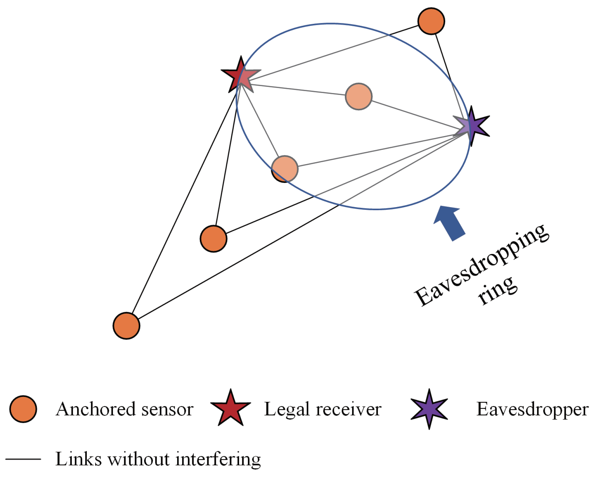
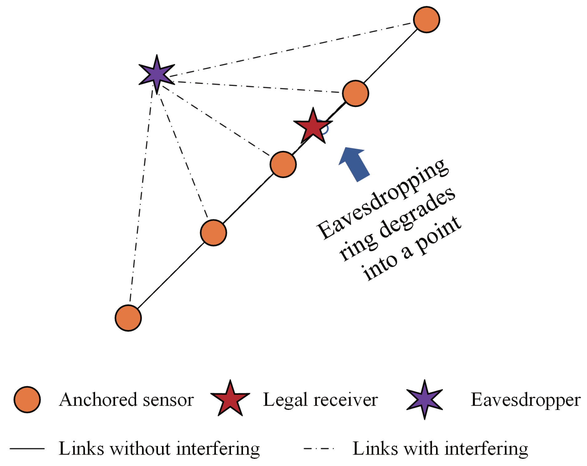
The collector can achieve the maximal throughput at arbitrary locations while adopting the TRAS-MAC protocol described in Section 2.2. However, if the collector is located outside the one-dimensional space of the sensor nodes’ chain, an eavesdropping ring centered on these linearly deployed sensor nodes exists, as illustrated in Figure 8. The radius of the eavesdropping ring is equal to the vertical distance from the legal receiver to the sensor node chain. Owing to the symmetry, the distance from an arbitrary position in the eavesdropping ring to sensor node $n_i$ also equals $d_i$. Therefore, the receiving-alignment toward the legal receiver also means receiving-alignment toward any unintended receiver located in the eavesdropping ring.

In this sense, if the collector’s location is exposed to the eavesdropper, the adversary eavesdropper can easily find the eavesdropping ring and move to any position in there to steal all the reported data from the sensor nodes successfully.

It is noted that the channel is occupied by the two-way handshake between the collector and a sensor node during the first notification stage. In this case, unfortunately, an adversary eavesdropper can successfully receive the broadcasting 1st-Ini packet and decode the scheduled sending time of the sensor node. According to (3), the distance difference for the sequential sensor nodes can be deduced through the sending time $T_i$ as follows:

$$\begin{array}{ccc}{d}_{o_2}-d_{o_1}& =& v\left(T_{o_1}-T_{o_2}+T_f\right)\\ d_{o_3}-d_{o_2}& =& v\left(T_{o_2}-T_{o_3}+T_f\right)\\ ⋮& ⋮& ⋮\\ d_{o_N}-d_{o_{N-1}}& =& v\left(T_{o_{N-1}}-T_{o_N}+T_f\right).\end{array}$$

(4)

According to localization theory, the eavesdropper can obtain the eavesdropping ring centered around the sensor node chain based on the time difference of arrival (TDOA) information in (4) and the location of anchored sensor nodes. In the worst case, if the locations of anchored sensor nodes have been acquired by the eavesdropper, the eavesdropper can deduce the eavesdropping ring, move there, and eavesdrop all the reported data successfully.

3.1.2. Solution and Analysis toward Anti-Eavesdropping

It is noted that the radius of the eavesdropping ring is the vertical distance from the legal collector to the sensor node chain. Therefore, moving the collector into the one-dimensional space of the sensor node chain can force the eavesdropping ring to degrade into a single point, which is exactly the collector’s location. As shown in Figure 9, it is impossible for the eavesdropper to find a location that can successfully receive all the reported data without collision.

As the collector and the sensor nodes are located in the same one-dimensional space, the distance $d_i$ can be expressed as

$$d_i=\left\{\begin{array}{cc}\overline{l}+\frac{(i-1)l}{2},\hfill & imod2=1,\hfill \\ l-\overline{l}+(\frac{i}{2}-1)l,\hfill & imod2=0,\hfill \end{array}\right.$$

(5)

where $\overline{l}$ denotes the distance from the collector to $n_1$, $\overline{l}\le \frac{l}{2}$, and we have $d_1=\overline{l}$.

Actually, as if the eavesdropper is also located inside the one-dimensional space of the sensor nodes chain, we have the following findings regarding the anti-eavesdropping ability. First, there is the the impact of the arrival order.

Proposition 1.

The CD-EA and FD-EA orders illustrated in Figure 5 outperform the other arrival orders in anti-eavesdropping.

Proof. 

For these two arrival orders, i.e., CD-EA and FD-EA, the senders of two arbitrary neighboring arrival packets are located on two different sides of the receiver. Therefore, as the packet arrives in the eavesdropper, which is also located in the one-dimensional chain, continuous collisions are supposed to happen between two arrival packets, and the proof is completed. □

Second, there is the impact of the parity of the value of N.

Proposition 2.

The even network can cause more collisions in the eavesdropper than the odd network when using CD-EA or FD-EA orders.

Proof. 

As we know from Proposition 1, continuous collisions are supposed to happen between two arrival packets while using CD-EA or FD-EA orders. In this sense, all the reported packets will collide in the eavesdropper as N in an even value. However, there is the possibility that one packet during a transmission period does not interfere with the other arrived packets as N is an odd value, and the proof is completed. □

In this sense, the adversary is better off deploying multiple eavesdroppers in different locations outside the one-dimensional chain to increase its eavesdropping probability.

3.2. Exposure of the Collector’s Location

As discussed above, the eavesdropper cannot precisely locate the collector’s location in the eavesdropping ring if the collector is outside the one-dimensional space formed by the sensor node chain. Although moving the collector into the one-dimensional space can highly promote the anti-eavesdropping ability, the position of the collector will be exposed to the eavesdropper subsequently.

The exposure of the collector’s location can be attributed to two main reasons. First, the floor acquisition of the channel during the notification stage enables the eavesdropper to receive all the 1st-Ini packets successfully. Second, the relative spatial information is embedded inside the transmission strategies and broadcast through the 1st-Ini packet. On these bases, if the location of the anchored sensor nodes is exposed to the eavesdropper, the one-dimensional location of the collector can be easily deduced. Then, the collector is directly threatened by tracking or even an attack.

The slotting technique is promising to solve the exposure problem. On the one hand, when using slotted accessing, sensor nodes only need to transmit their collected data at the beginning of each slot without any additional activities required. Therefore, the collector only needs to broadcast the common transmission strategy (i.e., slot length and the packet duration) instead of notifying each sensor node of their specific transmission time. On the other hand, the slotting technique can erase the relative distance information from the broadcast transmission strategies, which protects the location privacy of the collector.

However, achieving receiving-alignment at the receiver is more challenging when using the slotting technique, as will be discussed in the next section.

4. SRAS-MAC: Slotted- and Receiving-Alignment-Based Scheduling MAC

In this section, we first study achieving the receiving-alignment in the receiver while using the slotting technique and further design the SRAS-MAC. Then, we discuss why the proposed SRAS-MAC can protect the location privacy of the collector. We further give an overview of the proposed SRAS-MAC protocol.

4.1. Spatial Reuse through Slotting Accessing

Let $T_{slot}$ denote the slot length, which is given as

$$T_{slot}=T_f+\beta T_d,$$

(6)

where $T_d$ denotes the maximal propagation delay from the sensor nodes to the collector and $\beta$ is a guard coefficient, which satisfies $0\le \beta \le 1$. In a star-connected network, collision-free regions (CFRs) exist when the slot length is greater than two-times the packet duration [9]. In this sense, the slot length setting should satisfy the following condition so as to achieve spatial reuse:

$$2T_f<T_{slot}\le T_f+T_d.$$

(7)

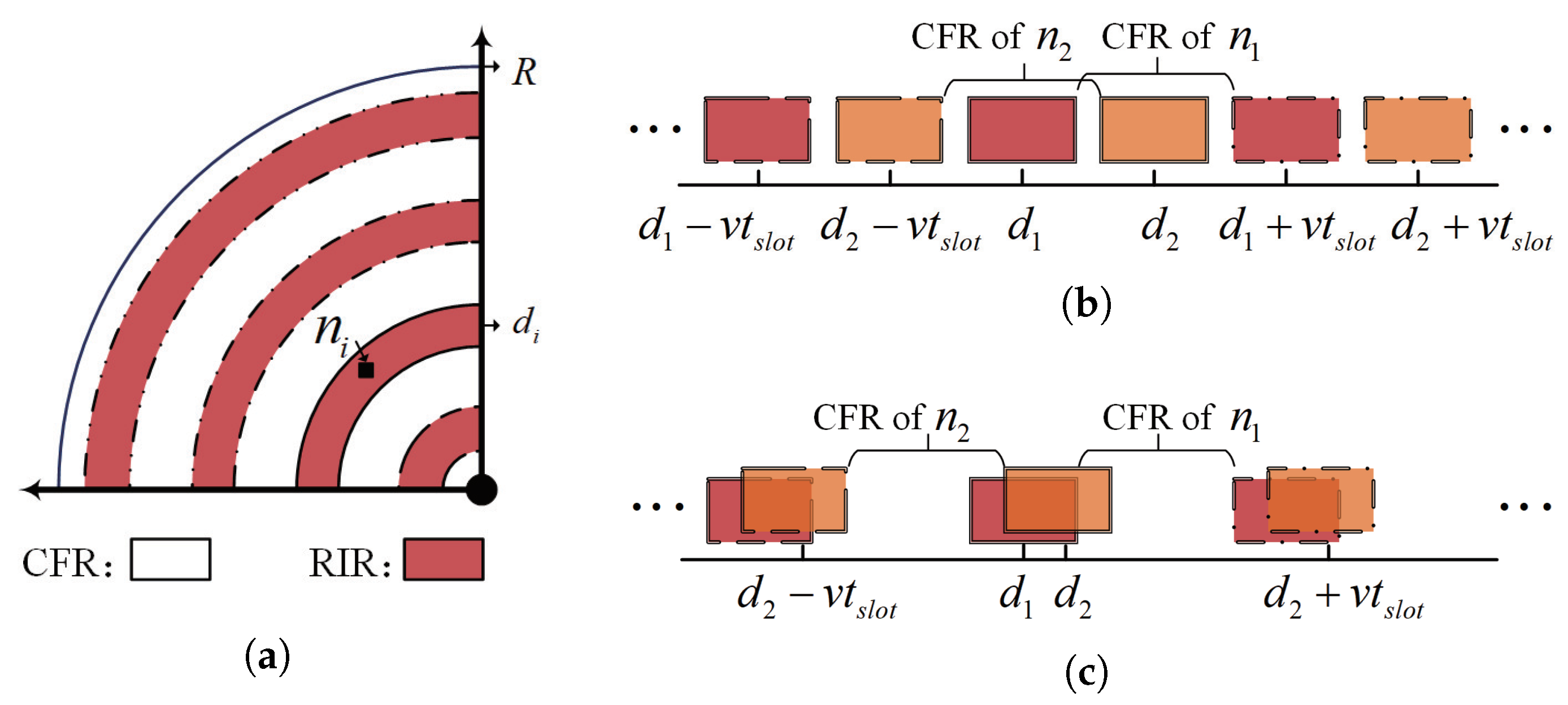
As shown in Figure 10a, the CFRs corresponding to a tagged sender are a group of concentric annuli centered on the receiver and inside the coverage of the receiver. It is noted that, except for the CFRs at two ends, the width of each CFR is equal to $v(T_{slot}-T_f)$, and the locations of the corresponding CFRs of each sender are determined by $d_i$ and $T_{slot}$.

We take two sensor nodes (i.e., $n_1$, $n_2$) as examples to discuss how to exploit the CFRs so as to achieve spatial reuse while using the slotting technique. We assumed $n_1$ and $n_2$ are fully loaded and going to access the channel at each slot. As shown in Figure 10b, $n_1$ and $n_2$ are located at the CFRs of each other. In this case, the simultaneously transmitted packets from $n_1$ and $n_2$ will not collide at the receiver, which achieves spatial reuse. On the contrary, it is also possible that these two nodes keep interfering with each other because they are located outside each other’s CFRs, as shown in Figure 10c.

The examples illustrated in Figure 10 suggest an opportunity to achieve spatial reuse by adjusting the relative distance difference $d_i-d_j$ among the senders to the receiver. Since the sensors are anchored, it is better to adjust the relative distances from the receiver side. This inspired us to find suitable locations for the collector where spatial reuse among sensor nodes can be achieved. At the same time, a corresponding design of the time slot is also required to achieve optimal channel utilization.

4.2. Design of SRAS-MAC

Let k denote the order of the slots and $T_{S_k}$ denote the beginning time of the k-th slot, which can be expressed as

$$T_{S_k}=(k-1)T_{slot},k\in {\mathbb{N}}^{+}.$$

(8)

Since the sender can only send a data packet at the beginning of each slot, each sender at most has one packet arrive at the receiver during a period equal to $T_{slot}$.

Proposition 3.

Supposing node $n_1$ sends a packet at slot k, for the other packets arriving at the receiver from time $\frac{d_1}{v}+T_{s_k}$ till time $\frac{d_1}{v}+T_{s_{k+1}}$, their sending slot is before slot $k+1$.

Proof. 

Assuming a packet is sent from $n_i$ at $\widehat{k}$ slot, its arrival time satisfies

$$\frac{d_1}{v}+T_{S_k}<\frac{d_i}{v}+T_{S_{\widehat{k}}}<\frac{d_1}{v}+T_{S_{k+1}},$$

(9)

where $\forall i\in \{1,\dots ,N\}$ and $\widehat{k}\ge k+1$. The left side of (9) is always satisfied. However, based on the right side of (9), the difference between the sending slot and sending position should satisfy the condition as

$$T_{S_{\widehat{k}}}-T_{S_{k+1}}<\frac{d_1-d_i}{v}.$$

(10)

The upper-bound and lower-bound of the two sides in (10) are given as follows:

$$T_{S_{\widehat{k}}}-T_{S_{k+1}}\ge 0,\frac{d_1-d_i}{v}\le 0.$$

(11)

Since the condition in (11) contradicts (10), the proof is completed. □

Let $m_i$ denote the sending slot difference between $n_1$ and the other nodes. According to (8) and Proposition 3, $m_i$ can be expressed as

$$m_i=⌈\frac{d_i-d_1}{v{T}_{slot}}⌉-1,i\in \{1,\dots ,N\}.$$

(12)

Based on (12), taking $n_1$ as the reference node, the distance $d_i$ can be transformed into ${\widehat{d}}_i$ as follows:

$${\widehat{d}}_i=d_i-v{m}_i{T}_{slot}-d_1,0\le {\widehat{d}}_i\le v{T}_{slot}.$$

(13)

Using the transformed distance ${\widehat{d}}_i$ in (13), we only need to solve the scheduling problem within one slot. The transformed ${\widehat{d}}_{i}v$ is the arrival time of those packets in the slot. Similar to the protocol model shown in (2), based on the transformed distance (13), the collision-free condition in a slot can be written as follows:

$$\left|\frac{{\widehat{d}}_i-{\widehat{d}}_j}{v}\right|\ge T_f,i\ne j.$$

(14)

It is noted that, for arbitrary two nodes j and k that satisfy $d_j\le d_k$, it does not mean ${\widehat{d}}_j\le {\widehat{d}}_k$.

As shown in Equations (12) and (13), given the slot length, adjusting the collector position will change the arrival order of packets sent by sensor nodes. On the contrary, we can also first select an arrival order of packets (e.g., ${\widehat{d}}_i/v$) to satisfy (14) and, then, try to find an achievable location for the collector that satisfies the selected arrival orders. Furthermore, in order to achieve maximal throughput, we want to find a perfect location for the collector under the minimum slot length.

Since all the senders periodically send their packets with interval $T_{slot}$, N data packets at most are sent to the receiver in $T_{slot}$ time. Therefore, the minimum slot length is given as follows:

$$T_{slot}=N·T_f.$$

(15)

We selected the CD-EA order to achieve receiving-alignment at the receiver since it is proven in Proposition 1 that it can achieve higher anti-eavesdropping ability. The ${\widehat{d}}_i$ under CD-EA order can be expressed as follows:

$${\widehat{d}}_{i}v=(i-1)·T_f,i\in \{1,\dots ,N\}.$$

(16)

Proposition 4.

To achieve the receiving-alignment shown in (16), the distances’ set {$d_i\},1\le i\le N$, should strictly satisfy

$$d_1<d_2<\dots <d_N.$$

(17)

Proof. 

Assuming $d_i=d_{i+1}$, according to (13), the transformed distance satisfies

$${\widehat{d}}_i={\widehat{d}}_{i+1},$$

(18)

which contradicts (14). Therefore, the proof is completed. □

According to (5), (13), and (16), $m_i{T}_{slot}$ should satisfy

$$v{m}_i{T}_{slot}=\left\{\begin{array}{cc}(i-1)\zeta ,\hfill & imod2=1,\hfill \\ (i-1)\zeta +\xi ,\hfill & imod2=0.\hfill \end{array}\right.$$

(19)

where $i\in \{1,\dots ,N\}$, $\zeta =\frac{l}{2}-v{T}_f$, and $\xi =\frac{l}{2}-2\overline{l}$.

Let $a|b$ denote that b is divisible by a. Therefore, the receiving-alignment (16) is achievable if $T_{slot}$ satisfies

$$\left(v{T}_{slot}\right)|\zeta ,$$

(20)

$$\left(v{T}_{slot}\right)|\{(i-1)\zeta +\xi ,\forall i\in \{1,\dots ,N\}\}.$$

(21)

In (20) and (21), it is hard to find the common division of $\{\zeta ,(i-1)\zeta +\xi ,\forall i\in \{1,\dots ,N\left\}\right\}$.

Proposition 5.

When $\overline{l}$ is equal to $\frac{v{T}_f}{2}$ or $\frac{l}{4}$, the receiving-alignment (16) is achievable if (20) is satisfied.

Proof. 

When $\overline{l}$ is equal to $\frac{v{T}_f}{2}$, the $m_i{T}_{slot}$ can be expressed as follows:

$$v{m}_i{T}_{slot}=\left\{\begin{array}{cc}(i-1)\zeta ,\hfill & imod2=1,\hfill \\ i\zeta ,\hfill & imod2=0.\hfill \end{array}\right.$$

(22)

When $\overline{l}$ is equal to $\frac{l}{4}$, the $m_i{T}_{slot}$ can be expressed as follows:

$$v{m}_i{T}_{slot}=(i-1)\zeta .$$

(23)

In both (22) and (23), $\zeta$ always is the division of $v{m}_i{T}_{slot}$. Therefore, in these two positions, the receiving-alignment (16) can be achieved as long as (20) is satisfied, which completes the proof. □

Based on Proposition 5 and (15), in order to satisfy the condition in (20), we can adjust the packet duration as follows:

$$T_f=\frac{l}{2v\left(N·z+1\right)},$$

(24)

where $z\in \{0,{\mathbb{N}}^{+}\}$. Let B denote the packet size (in Byte), which is determined by $T_f$ as follows:

$$B=⌈T_f·r/8⌉,$$

(25)

where r denotes the data rate of the acoustic modem (in bit/s).

4.3. Trade-Off between Anti-Eavesdropping and Location Privacy of Collector

Proposition 5 has given two special $\overline{l}$ (i.e., $\overline{l}=\frac{v{T}_f}{2}$ and $\overline{l}=\frac{l}{4}$) for the receiver that can achieve receiving-alignment using the slotting technique. Due to the symmetry of the topology, four optional locations are available for the collector. In this case, the eavesdropper cannot distinguish which one is the final choice of the collector, and the risk of the location being exposed is reduced from 100% to 25%.

Basically, the greater $T_f$ leads to the greater $P_c$, so we intuitively want to use the greatest $T_f$ to achieve the highest $P_c$. As shown in (24), the maximal packet duration for SRAS-MAC is achieved by setting z in 0. However, as the z was set to 0, we have $\frac{v{T}_f}{2}=\frac{l}{4}$, which indicates that the number of available locations is halved into two available locations.

Therefore, a trade-off exists between anti-eavesdropping ability and the location privacy of the collector. If the location privacy of the collector is the primary object, z is better set to 1, and we have

$$T_f=\frac{l}{2v\left(N+1\right)},$$

(26)

where the probability of exposing the location of the collector is $\frac{1}{4}$. On the contrary, if the confidentiality of the reported data is the primary object, z is better set to 0, and we have

$$T_f=\frac{l}{2v},$$

(27)

where the probability of exposing the location of the collector is $\frac{1}{2}$.

4.4. The Overview of the SRAS-MAC Protocol

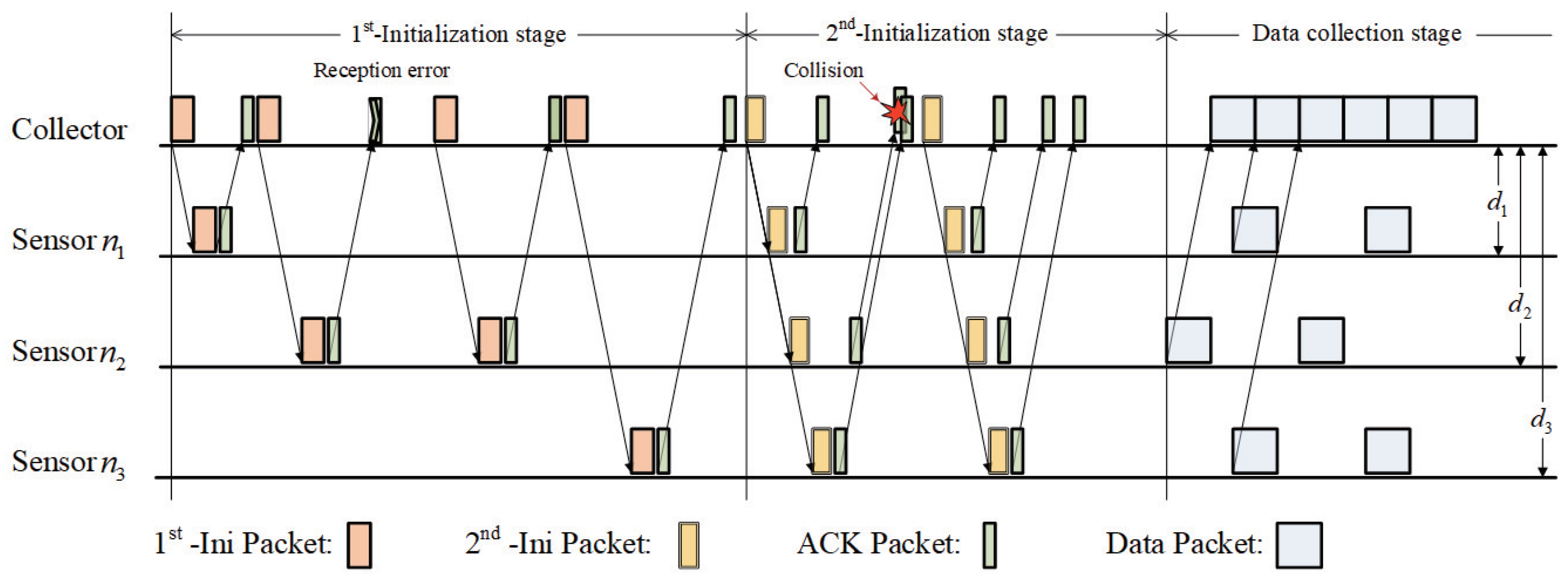
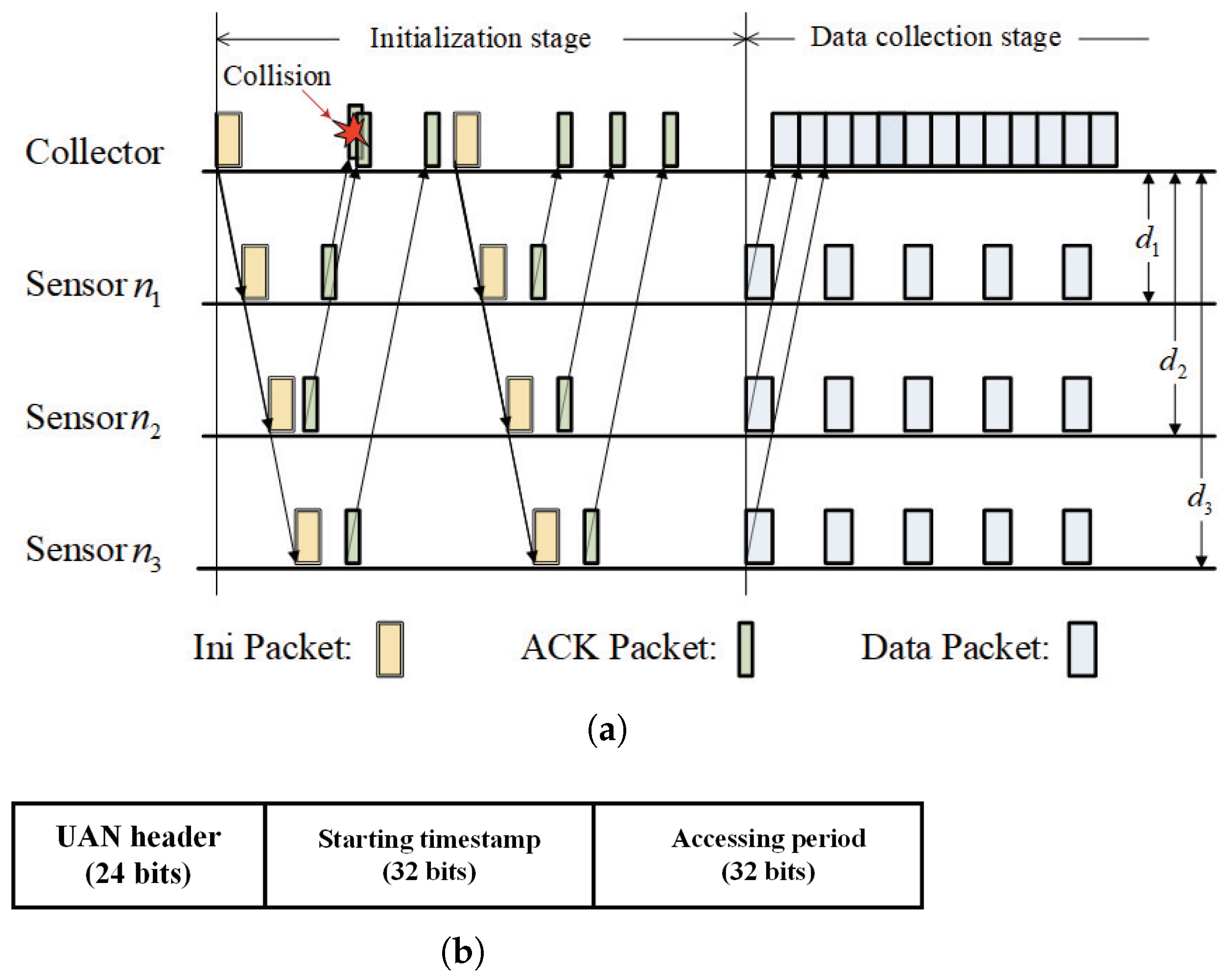
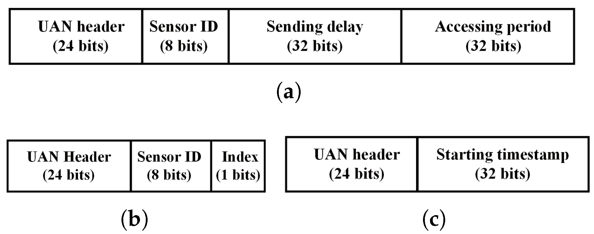
An example of the working process of the SRAS-MAC protocol is illustrated in Figure 11a. SRAS-MAC is also initiated by the collector. The collector first derives the packet duration based on (24). Then, it randomly selects one of the optional positions and moves there. As the collector has settled in the selected location, it activates the notification stage. The collector will assemble the beginning timestamp of the first slot and the accessing period into an Ini packet, whose structure is shown in Figure 11b.

The Ini packet will be broadcast to all sensor nodes, and the collector will wait for the acknowledgment from the sensor nodes. As a sensor node has successfully received the Ini packet, it will immediately update the accessing strategies and wait for a delay to send its ACK packet back to the collector. Owing to the regularity of these linearly deployed sensor nodes, the sensor node only needs to wait for a time greater than one duration of the Ini packet and can avoid the collision of the ACK packet and the Ini packet in the other sensor.

After waiting for two-times the maximal propagation delay, the collector will check whether it has successfully received the ACK packets from all the sensor nodes. If all the ACK packets have been successfully received, the collector is ready to receive the incoming reported data from the sensor nodes. Otherwise, the collector will renew an Ini packet and start the notification stage again.

5. Simulation Results

5.1. Simulation Settings’ Description

We used the NS-3 simulation results to evaluate the anti-eavesdropping abilities and time consumption of TRAS-MAC and SRAS-MAC in UANs. The underwater acoustic networks were modeled through the UAN module in the NS-3 simulator.

We propose the anti-eavesdropping ratio as a performance metric to evaluate the confidentiality of transmitted data and the anti-eavesdropping effect in the MAC layer. Let $P_c$ denote the anti-eavesdropping ratio, which can be calculated as

$$P_c=1-\frac{N_e}{N_s},$$

(28)

where $N_e$ is the number of reported packets successfully received by the eavesdropper and $N_s$ is the number of the total packets sent by all the sensor nodes.

In these simulations, the sensor nodes are linearly deployed with the same spacing distance l between two neighboring nodes, and their depth $l_d$ was fixed at 500 m. Each sensor node is equipped with a half-duplex acoustic modem whose data rate r was set at 2 kbps. During each simulation, each sensor node needs to deliver 100,000 B of data to the collector. For the SRAS-MAC, the collector’s location is randomly selected from four optional positions. For the TRAS-MAC, the collector’s location is randomly selected within the one-dimensional deployment area. The eavesdropper is randomly deployed within the one-dimensional or three-dimensional deployment area. We used UniFormRandomVariable provided by NS-3 to generate the coordinates of the collector in TRAS-MAC and the eavesdroppers. Each simulation result is the expectation based on 1000 runs of simulations.

5.2. The Impact of Arrival Order and Parity of N to $P_c$

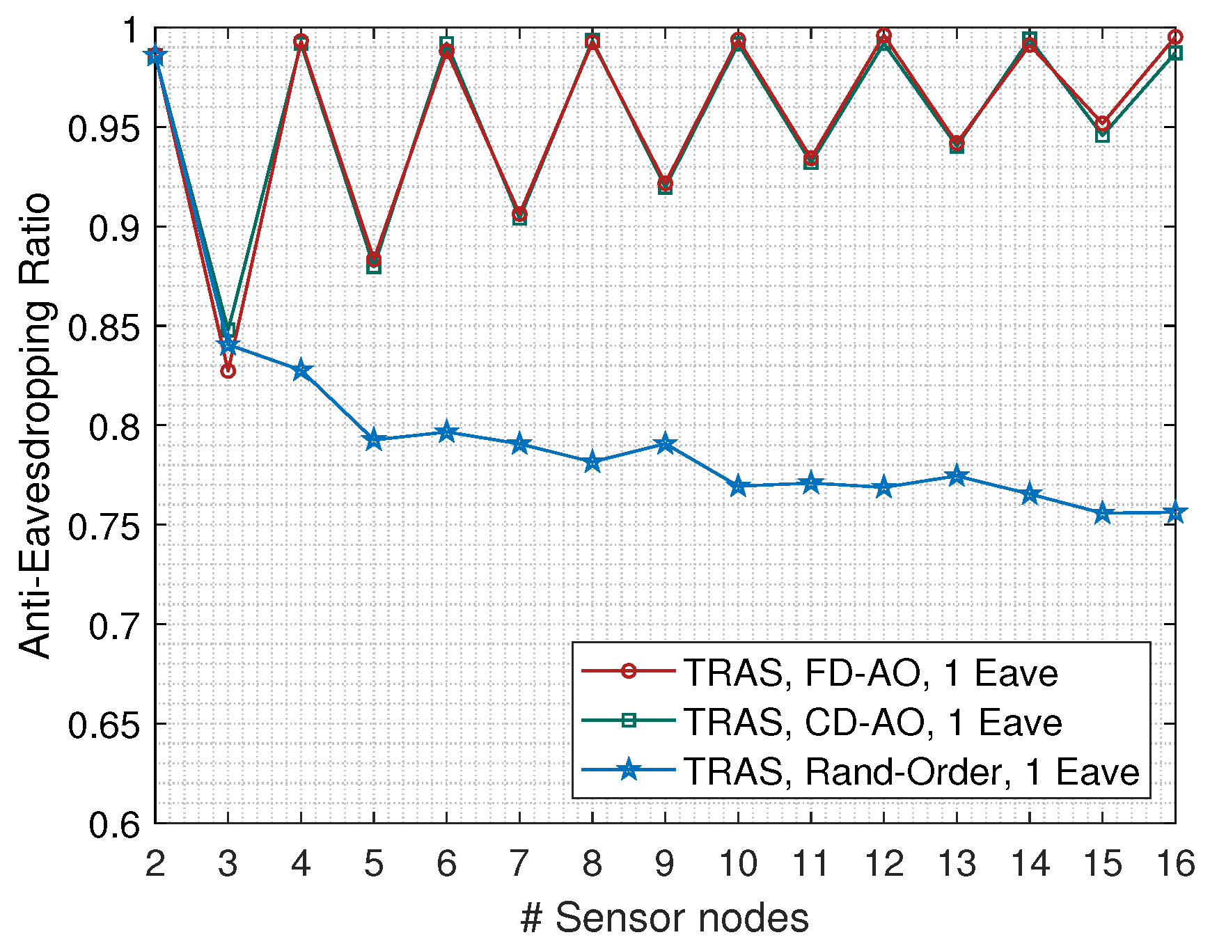
First, we discuss the impact of the arrival order and the parity of N to the anti-eavesdropping ratio $P_c$ of TRAS-MAC. The selected arrival order of receiving-alignment includes “CD-EA”, “FD-EA”, and random order. In this discussion, the eavesdropper is also deployed within the one-dimensional deployment area. The spacing distance l was set at 15 km, and the packet size B was fixed at 125 B.

From Figure 12, we can observe that the TRAS-MAC with random arrival order had a lower performance compared to the TRAS-MAC with the CD-EA or FD-EA order, which both achieved similar $P_c$ values for a given N. Hence, Proposition 1 is validated. Then, as illustrated in Figure 12, the parity of N had the same impact on the value of $P_c$ under both CD-EA or FD-EA orders. Specifically, TRAS-MAC performed better when N was an even value than when N was an odd value. Hence, Proposition 2 is also validated.

In addition, it is easy to notice that the $P_c$ was close to 1 for the TRAS-MAC under arbitrary arrival orders when $N=2$. According to (15), the slot length equaled two-times $T_f$ when $N=2$. Therefore, one slot duration was left in a scheduling period that was too short to tolerate the change of propagation delay toward the eavesdropper, resulting in almost all the overheard packets colliding with the eavesdropper. On the contrary, there was two-times the packet duration left when $N=3$, and there existed the possibility that one packet can be easily eavesdropped at the eavesdropper when the N was an odd value. Hence, we can observe that the value of $P_c$ greatly decreased from $N=2$ to $N=3$.

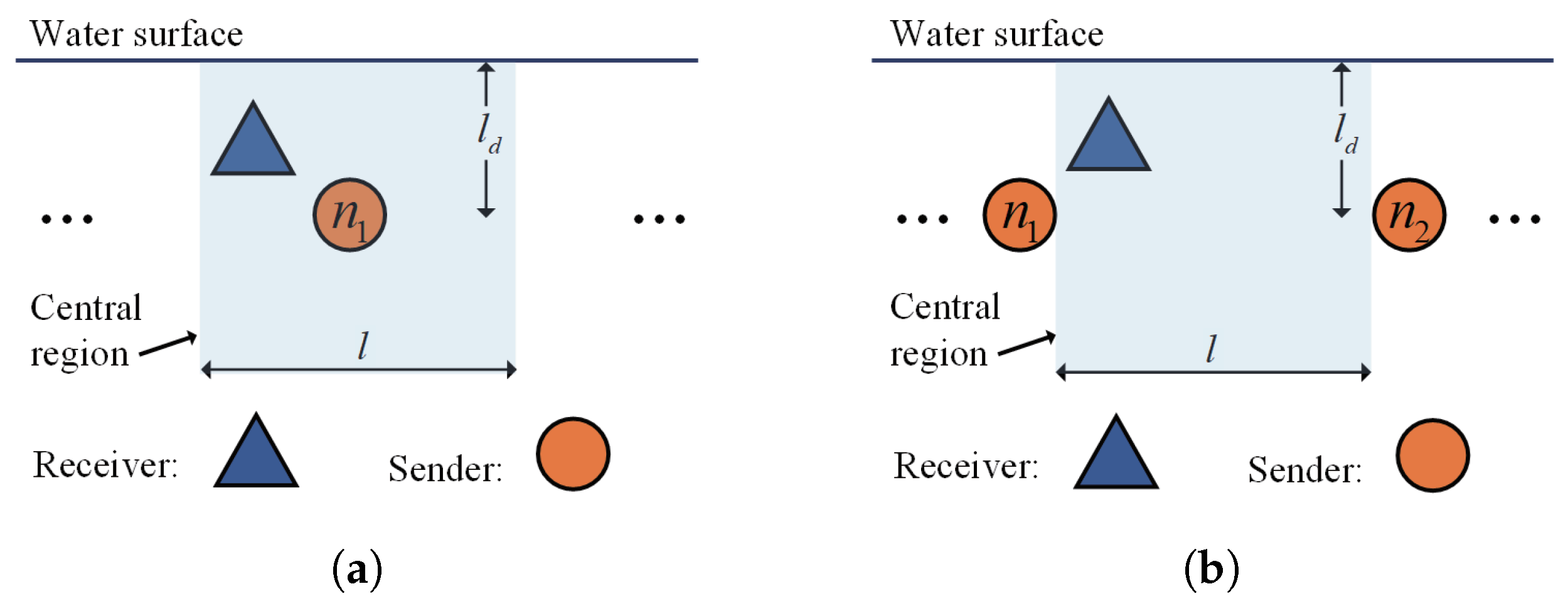
The simulation results illustrated in Figure 12 have shown that the eavesdropper was constrained when it was located within the one-dimensional space, i.e., almost a few data can be eavesdropped for the case that N was an even value. In the following discussions and evaluations, the eavesdroppers were randomly located within the central region with size $l\times l\times 2l_d$, as shown in Figure 3.

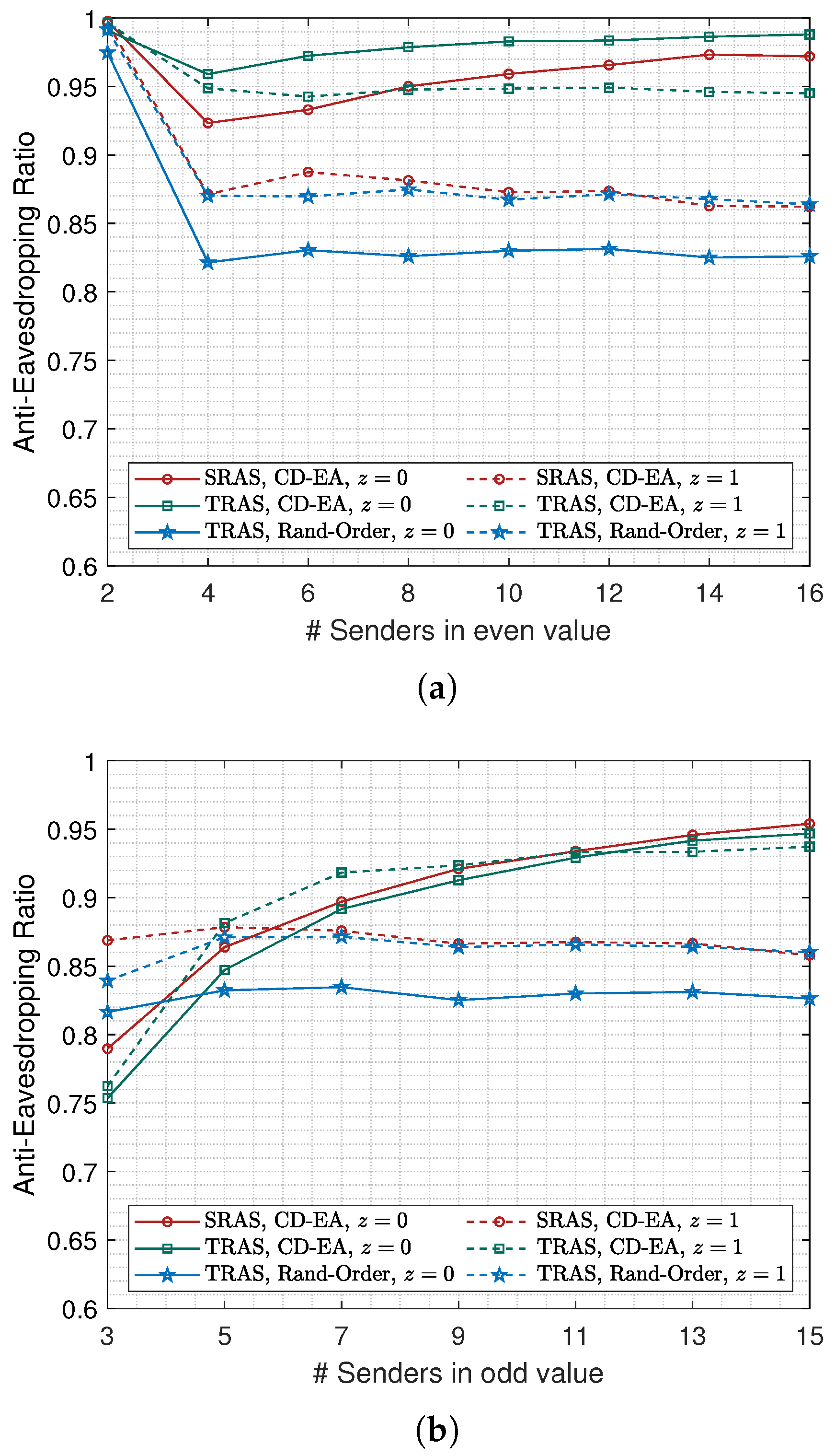
5.3. The Impact of Packet Duration $T_f$ to $P_c$

As discussed in Section 4.2, SRAS-MAC needs to adjust the packet duration to achieve collision-free receiving-alignment, and there is a trade-off between the anti-eavesdropping ability and the location privacy of the collector. In this discussion, the spacing distance l was also set at 15 km, and the packet duration of SRAS-MAC and TRAS-MAC was set according to (26) and (27) for $z=1$ and $z=0$, respectively.

Considering the impact of parity of N, as we discussed in Section 5.2, the $P_c$ under the network that N is an even value and N is an odd value are illustrated in Figure 13a,b, respectively.

As shown in Figure 13a, $P_c$ was still close to 1 for both SRAS-MAC and TRAS-MAC under arbitrary arrival orders and arbitrary values of $T_f$ when $N=2$, whose reason has been discussed above. Also, we noticed that, for the case of setting z to 0, the achieved $P_c$ of SRAS-MAC and TRAS-MAC using the CD-EA order still grows as the value of N increases in Figure 13a,b, respectively. Moreover, it is noticed in Figure 13b that SRAS-MAC outperforms the TRAS-MAC in $P_c$ when the value of N is in 13 and 15.

Then, for the SRAS-MAC and TRAS-MAC under the CD-EA order, we can observe that they achieved greater $P_s$ in most cases where z was 0 than in cases where z was 1. On the contrary, for the TRAS-MAC under random arrival order, the achieved $P_s$ performed worse when z was 0 than when z was 1. It can be understood that the longer time slot while setting z in 0 will result in a greater spatial reuse opportunity. As we discussed in Proposition 1, using the CD-EA order can efficiently constrain the spatial reuse opportunity, but not using the random arrival order.

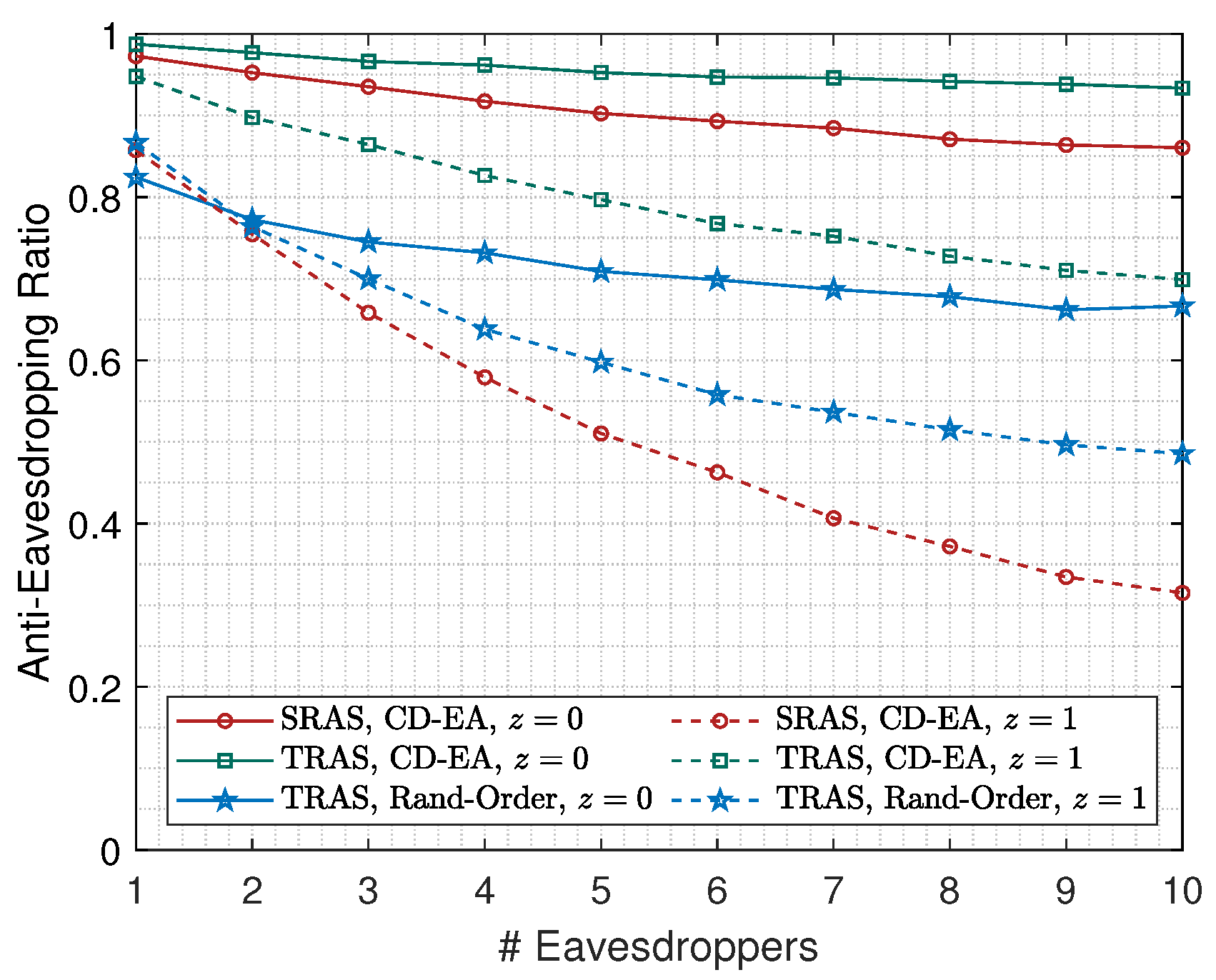
5.4. The Impact of the Number of Eavesdroppers to $P_c$

As shown in Figure 13, for the only one-eavesdropper case, the available $P_c$ of SRAS-MAC and TRAS-MAC were always over 0.75. Moreover, for SRAS-MAC, at most three fake collector locations existed. Therefore, we were interested in studying the anti-eavesdropping abilities of multiple eavesdroppers.

We illustrate the values of $P_c$ encountering an increasing number of eavesdroppers (i.e., from 1 to 10) in Figure 14, where l was set to 15 km, N was set to 16, and the eavesdroppers were still randomly located within the three-dimensional deployment area.

It is clear that the more eavesdroppers join the network, the lower the $P_c$ that can be achieved. However, the SRAS-MAC and TRAS-MAC with the CD-EA arrival order z set to 0 still achieved 0.8 in $P_c$ under the cases where ten eavesdroppers were located inside the deployment area. On the contrary, compared to the case of z set to 0, the anti-eavesdropping ratio of the other schemes declined more quickly setting z to 1. It is noted that, as the eavesdroppers increased to four, about 60% of the data could still be saved using SRAS-MAC with z set to 1. Since it is hard to guarantee the location privacy of the collector even in SRAS-MAC, as the number of eavesdroppers was greater than four, it was better to use the maximal packet duration ($z=0$) to maximize the security of the reported information.

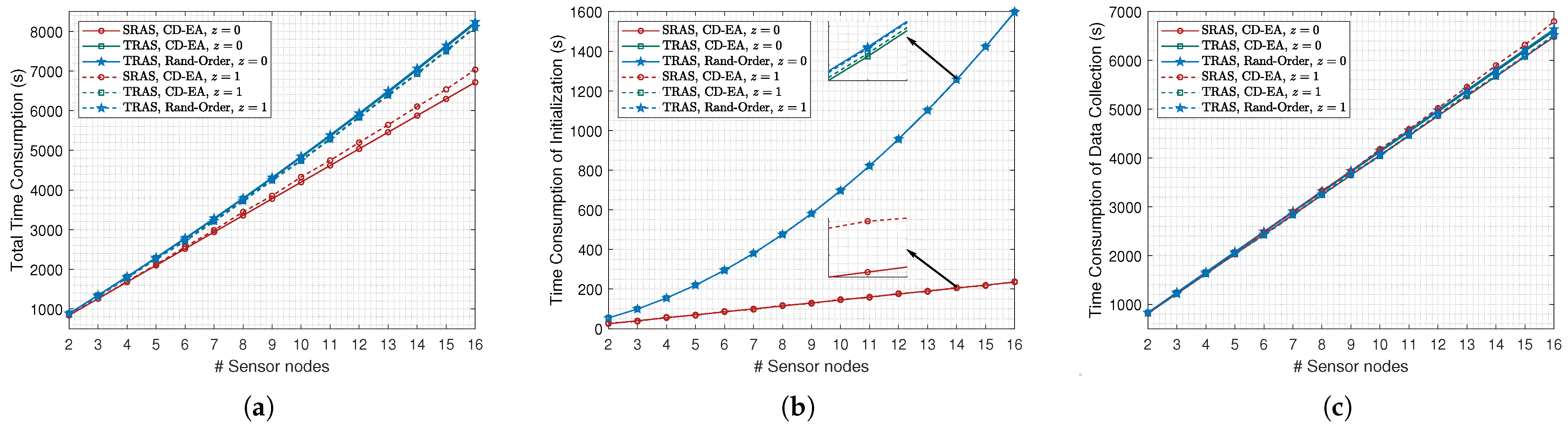
5.5. The Impact of l and N on the Time Consumption

Finally, we want to discuss the time consumption among SRAS-MAC and TRAS-MAC with different packet duration settings. The values of the time consumption were calculated as follows:

• The total time consumption: from the time that the collector sent the first control packet to the time that the collector received the last reported data packet.
• The time consumption of data collection: from the time that one of the sensor nodes sent the first data packet to the time that the collector received the last reported data packet.
• The time consumption of initialization: the difference between the total time consumption and the time consumption of data collection.

For the simulation with different settings of N, which was from 2 to 16, l was set to 15 km, and the results are illustrated in Figure 15. As shown in Figure 15a, the TRAS-MAC protocol consumed more time collecting the same size of data and increased more quickly as the value of N grew. Specifically, for the case that $N=16$, the TRAS-MAC protocol consumed a quarter more time than the SRAS-MAC protocol. The reason can be found in Figure 15b. Since an extra two-way handshake existed between the collector and each sensor node, the time consumption during the initialization of the TRAS-MAC protocol was much greater than the SRAS-MAC protocol and grew more quickly as the value of N grew. On the contrary, as shown in Figure 15c, there was little difference between the TRAS-MAC protocol and the SRAS-MAC protocol in the time consumption during data gathering.

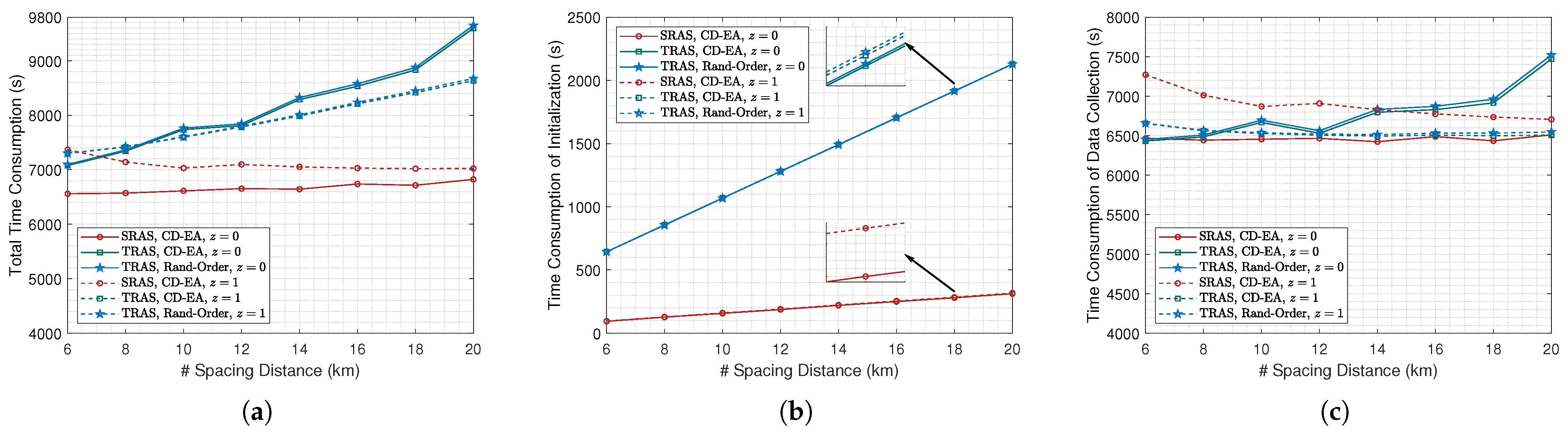
For the simulation results for different settings of l, i.e., from 6 km to 20 km, N was set at 16, and the results are illustrated in Figure 16. Similar to the results in Figure 15, as illustrated in Figure 16a, the total time consumption of the TRAS-MAC protocol was greater than the SRAS-MAC protocol. However, it can be observed that the total time consumption of the TRAS-MAC grew as the value of l increased. In the same cases, the total time consumption of the SRAS-MAC remained stable. However, the difference can be found in the initialization and data-collection stages. As shown in Figure 16b, the time consumption of the TRAS-MAC protocol during initialization increased more quickly than the SRAS-MAC protocol as the value of l increased. Moreover, as shown in Figure 16c, the time consumption of the data collection of the TRAS-MAC setting z to 0 also increased as the value of l increased, which led to greater total time consumption.

6. Conclusions

This paper is the first work to reveal the security nature of space–time coupling access in UANs. We studied this in a data-gathering scenario in which a group of linearly deployed sensor nodes directly sends their packet to a single receiver. We discovered an eavesdropping ring centered on those deployed sensor nodes, where the eavesdropper can successfully steal all the reported packets. We found that the typical receiving-alignment-based scheduling MAC (TRAS-MAC) exposed the relatively spatial information among sensor nodes with the collector to the eavesdropper, which enabled the eavesdropper to locate the eavesdropper ring and steal all the reported data. We discovered that the eavesdropping ring could be degraded into a point by deploying the collector within the one-dimensional space of the linear sensor node chain, which alleviates the eavesdropping risk. However, the collector’s location will be exposed to the eavesdropper, and its security is at risk. We proposed a slotted- and receiving-alignment-based scheduling MAC (SRAS-MAC) protocol, which can provide at most four optional positions to the collector to hide its location. The analysis and the simulation results showed that using closer distance, earlier arrival and farther distance, earlier arrival orders can efficiently prevent the data from being eavesdropped when the eavesdropper is also located inside the one-dimensional deployment area. We also found that the eavesdropper can steal fewer packets as if the number of sensor nodes is an even compared to an odd value. Further evaluations of the packet duration and the number of eavesdroppers when the eavesdropper is located inside the three-dimensional deployment area were conducted through NS-3 simulations. The simulation results showed that, if the maximal packet duration is adopted, the proposed SRAS-MAC achieved similar anti-eavesdropping performance as TRAS-MAC using the CD-EA order. Moreover, SRAS-MAC can efficiently prevent eavesdropping attacks from multiple eavesdroppers, e.g., less than 20% of the data can be stolen under the ten-eavesdropper case. The simulation results also showed that SRAS-MAC performed better than TRAS-MAC in the time consumption.

In future work, on the one hand, we plan to analyze the anti-eavesdropping ability under a more-general topology and design anti-eavesdropping scheduling protocols accordingly; on the other hand, we will consider exploring the applicability and robustness of the proposed SRAS-MAC protocol through field tests.