A Novel Unmanned Surface Vehicle Path-Planning Algorithm Based on A* and Artificial Potential Field in Ocean Currents

Abstract

Ocean currents make it difficult for unmanned surface vehicles (USVs) to keep a safe distance from obstacles. Effective path planning should adequately consider the effect of ocean currents on USVs. This paper proposes an improved A* algorithm based on an artificial potential field (APF) for USV path planning in a current environment. There are three main improvements to the A* algorithm. Firstly, the proposed algorithm ignores unnecessary perilous nodes to decrease calculation. Secondly, an adaptive guidance angle is developed to guide the search in the most appropriate direction to reduce the computing time. Thirdly, the potential field force function is introduced into the cost function to ensure that the path designed for the USV always maintains a safe distance from obstacles under the influence of ocean currents. Furthermore, the Bezier curve is adapted to smooth the path. The experimental results show that the USV path-planning algorithm proposed in this paper, which synthesizes the APF and A* algorithms, runs 22.5% faster on average than the traditional A* algorithm. Additionally, the path developed by the proposed A* algorithm effectively keeps appropriate and different distances from obstacles by considering different ocean currents.

1. Introduction

An unmanned surface vehicle (USV) is a novel intelligent vessel equipped with self-governing perception, planning, and navigation technology [1]. Due to its diminutive size and superior maneuverability, it is extensively applied in maritime transportation, patrolling, and rescue. With the advancement of science and technology and the proliferation of practical applications, global path planning for USVs in intricate environments has also become a focal point of research [2].

The essence of path planning involves discovering a collision-free route from the starting point to the endpoint on a map. Path planning technology is particularly crucial as a pivotal aspect of intelligent technology for USVs. It is a fundamental facet of the research on intelligent devices such as intelligent robots, intelligent vehicles, USVs, and autonomous underwater vehicles (AUVs). The path planning for USVs is mainly categorized into global path planning based on map information and local path planning based on the real-time navigational environment and state [3].

Recent studies highlight the crucial need to consider ocean currents in path planning for USVs [4,5]. Ocean currents significantly impact path optimization and trajectory tracking, directly influencing the efficiency and safety of USV navigation [6]. Once the path planning for a USV is completed, further validation of the algorithmically planned path’s rationality can be achieved through simulation-based path tracking and empirical verification [7]. The primary technical foundation for the execution of diverse surface operations by USVs is trajectory tracking [8]. It mainly explores how a USV follows the planned path and proves the effectiveness of the proposed path-planning method. Trajectory tracking encompasses the formulation of a control mechanism enabling USVs to adhere to a specified, time-varying trajectory commencing from a predefined initial state [9]. Recently, numerous control strategies, such as PID control, neural network control (NNC), and model predictive control (MPC) [10,11] have been adapted to tackle the challenge of the path tracking of USVs in complex ocean environments [12]. Since the primary focus of this study is on global path planning for USVs, only a brief overview of trajectory tracking is provided.

The movement of a USV is subjected to wind, waves, currents, and other surrounding conditions. Ocean currents are one of the most influential factors that adversely affect a USV’s ability to follow the preset path safely and keep an appropriate distance from obstacles. Therefore, it is of great importance to consider ocean currents during path planning for a USV. This paper proposes an enhanced A* algorithm, which considers ocean currents with a potential field force to keep a safe distance from obstacles. In comparison with the traditional A* algorithm, the contributions of this paper are as follows:

(1)

The search strategy of the A* algorithm is enhanced by incorporating the elimination of perilous nodes and the adaptive guidance angle to enhance the computation efficiency. Additionally, the concept of an artificial potential field (APF) is integrated into the cost function of the traditional A* algorithm as a cost weight.

(2)

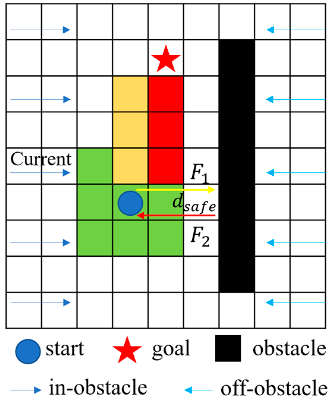
The effect of ocean currents is computed with the virtual potential field force exerted by the obstacle on the USV. When the force of the ocean currents propels the USV toward an obstacle, the equivalent force produced virtually by the obstacle acts as a repulsive force, which causes a path to be generated to steer clear of the obstacle. On the contrary, the planned path points can be selected to be close to the grid nodes near the obstacles. This is achieved by introducing equivalent forces to mitigate the adverse effects of the ocean currents.

(3)

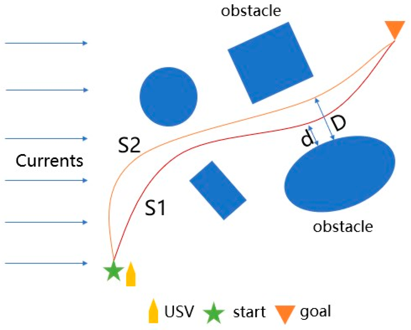
The path planned by the improved A* algorithm can maintain a safe and appropriate distance from obstacles under various current conditions. This provides a sufficient safety margin for the actual navigation of the USV to mitigate the adverse effects of ocean current disturbances. Furthermore, this research allows the influence of ocean currents to be taken into account in the path-planning phase, thereby providing a safer margin for the path-tracking and control phase.

This paper is organized as follows. Section 2 provides a literature review on path planning. Section 3 describes the methodologies for constructing the environmental model in currents and improving the A* algorithm. Section 4 presents experiments and a numerical analysis. Section 5 summarizes the research content of this paper and further research.

2. Literature Review

Recently, there has been a lot of research in the field of path planning for USVs considering the effect of ocean currents [13,14], focusing on energy consumption, planning time, path length, and path safety [15]. This section briefly overviews the A* algorithm and other prevalent global path-planning algorithms. Furthermore, this paper summarizes the processing approaches and relevant algorithm enhancements for the path planning of USVs in an ocean current environment.

2.1. Global Path-Planning Methods

Popular global path-planning methods include graph search, random sampling, intelligent bionics, and combinatorial optimization [16]. Graph search algorithms mainly comprise the Dijkstra algorithm [17], the A* algorithm [18], and the D* algorithm [19]. These algorithms are relatively straightforward to compute and can yield an optimal path, but the path may contain numerous turning points. Hence, it is necessary to apply smoothing techniques to make the path feasible for a USV.

Random sampling algorithms are a category of sampling-based path-planning methods, such as rapidly exploring random trees (RRTs) [20] and probabilistic road maps (PRMs) [21]. These algorithms have worked well in practice for USVs and have shown the advantage of probabilistic completeness. Though these sampling-based algorithms have some drawbacks [22], various efforts have been made to improve them in the field of USVs [23]. Chi et al. [24] combined the Voronoi diagram with the RRT algorithm for path planning to enhance the sampling efficiency and guide the sampling direction. Moreover, Xu et al. [25] put forward the SMRS-RRT* algorithm, which simplifies the sampling area of the environmental map, accelerates the generation of initial paths, and enhances the algorithm’s operation efficiency.

Genetic algorithms (GAs), particle swarm optimization (PSO), and ant colony optimization (ACO) are classified as intelligent bionic algorithms [26]. Although these algorithms have a broad spectrum of applications, they are computationally intensive, slow to converge, and susceptible to becoming trapped in local optimal solutions.

Niu et al. [27] proposed a genetic algorithm that leverages Voronoi diagrams to generate energy-efficient paths for USVs in the current environment. Similarly, Lars et al. [28] utilized an evolutionary algorithm to calculate robot paths, significantly reducing the algorithm’s execution time. Bai et al. [29] proposed a plant growth route (PGR) algorithm, which guides USVs to avoid obstacles and reach target points through the magnitude of light intensity. Furthermore, the particle swarm-based path-planning algorithm is well-suited for complex environments in path planning [30].

The A* algorithm is a heuristic search algorithm, which combines the shortest path search of Dijkstra’s algorithm and the heuristic function. It is a widely used method for global path planning in grid maps for its computational simplicity and ease of implementation [31]. To meet the diverse requirements of various applications, numerous enhancements have been made to the original A* algorithm [32,33,34]. Daniel et al. [35] proposed a novel Theta* path-planning algorithm based on A* by smoothing the initial path generated.

The APF is another path-planning algorithm that adopts attractive and repulsive forces to steer objects away from obstacles and toward the goal point. The algorithm is computationally simple and is often combined with other path-planning algorithms for USVs, as proposed by Gan et al. [36]. Sang et al. [37] introduced an APF path-planning algorithm based on A* to realize the globally optimal sub-objective. It smooths and optimizes the path of a USV according to its dynamic characteristics. To plan a safer path with the shortest total length in a wind farm environment, Xie et al. [38] developed a multi-directional improved A* algorithm integrated with an APF. However, the path-planning APF method is prone to becoming trapped in local minima. To address this issue, Liu et al. [39] introduced a fast-marching method (FM) into the APF to escape the local minima. Zhou et al. [40] applied polygon guidance to an APF, which proved effective in a natural environment. Pan et al. [41] proposed a multi-objective hybrid path-planning algorithm combining A* with an APF to efficiently escape from the common local minimum and oscillations. It will be a promising trend to integrate various path search algorithms, such as genetic algorithms [42], the fast-marching method, and fuzzy APFs, to address the challenges of smart path planning.

2.2. Path Planning in the Current Environment

The conventional A* algorithm for path planning typically prioritizes the shortest path length or time. But for a USV at sea, the ocean currents should be considered in the path-planning stage to make the path more feasible and safer [43,44]. The energy consumption and safety resulting from ocean currents have received more attention from scholars worldwide [45,46].

To fully use the limited energy of a USV, Gao et al. [47] investigated ocean current modeling and utilized the vehicle’s energy consumption affected by ocean currents as a constraint function for the path-planning algorithm to avoid local current turbulence. Liu et al. [48] proposed an optimization algorithm based on a double penalty function that considers the dynamic coupling mechanism and energy consumption of a USV in an ocean current environment. Ma et al. [49] introduced a dynamically enhanced multi-objective particle swarm optimization (PSO) algorithm in an ocean current environment to plan multi-USV paths that consider the length, smoothness, economy, and safety of paths. Furthermore, Ma et al. [50] established a two-dimensional Lamb eddy current environment model. They constructed a hybrid fireworks–ant colony algorithm-based path-planning model, whose objectives include energy consumption, operation time, and path length. Xu et al. [51] proposed the Lazy Theta* algorithm based on environment optimization to reduce the energy consumption caused by ocean currents. The cost function incorporates the drift current angle and line-of-sight checking, which guides a USV to navigate in the current direction.

Considering the effect of ocean currents on the path of USVs, Yu et al. [52] proposed a traversal multi-target path-planning method for multiple USVs in space-varying ocean currents, which combined the Hungary algorithm and the virtual field RRT* (VF-RRT*) algorithm. Mahmoud Zadeh et al. [53] presented an uninterrupted collision-free path-planning system combined with a novel B-spline data frame and PSO, which facilitates the operational performance of USVs in an ocean-sampling mission. Zhao et al. [54] proposed the AENSGA-II to solve path planning for USVs in dynamically unforeseen situations, which can simultaneously optimize four objective functions (path length, smoothness, energy consumption, and path safety).

Liu et al. [55] established a model to assess the risk of obstacle collisions along the path of a UAV. This model assigns different risk values to obstacles such as currents, berths, lanes, and piers according to the extent of navigational impacts across all grid nodes. Then, the improved A* algorithm was designed to identify the nodes with the smallest risk value for path planning. Although this method guarantees safety, it often results in longer paths and a waste of waterway space. Xie et al. [56] considered the effects of currents, wind, and waves on ship speed when planning paths. However, the improved genetic algorithm may pose safety risks when planning the shortest path in complex waters.

In Ref. [57], a constrained A* algorithm was proposed. In a simulated ocean environment, the effects of static and dynamic obstacles were considered to generate a safer route by maintaining a safe distance. The study reduced the computation time and improved the operational efficiency by improving the heuristic function, which adapts to globally optimal path planning. Xie et al. [58] incorporated the effects of wind and wave currents into a ship’s movement model using MAKLINK graph theory. They combined Dijkstra’s algorithm and genetic algorithm to plan the shortest path of a USV. However, more work is needed to quantitively analyze the variation in the safe distance from obstacles influenced by various current conditions.

Despite a lot of research aimed at properly tackling ocean currents’ impacts on USV paths, there remains a study gap regarding USV path planning under varying current conditions [59]. We can explore path planning in a current environment in terms of the interaction that exists between USVs and currents. The safe distance that should be maintained between the path and obstacles is investigated according to the differences in the direction and speed of the currents.

Thus, this study aimed to address this gap by planning the shortest path while maintaining an appropriate safe distance for a USV by developing a novel, improved A* algorithm with a potential field force in different ocean currents. Additionally, the planned path is smoothed by the Bezier curve smoothing technique for enhanced efficiency.

3. Materials and Methods

In this section, we focus on the environmental map-modeling method based on grids and the effect of a current environment on the deviation in a USV’s track. Thus, an improved A* algorithm based on an APF is proposed in this study to solve the deviation in the USV’s track caused by ocean currents. Meanwhile, the improvements of the A* algorithm are explained in detail.

3.1. Environmental Model

3.1.1. Construction of the Environmental Map

The fundamental work of path planning is to develop an environmental map, which can be constructed by various methods such as the grid map, visual map, and topology methods. The grid method is widely adopted for the map modeling of path planning due to its simplicity and ease of implementation. Hence, this paper employed the grid method to construct the navigation environment map for a USV.

As the grid map method can adapt the grid size to actual requirements, the safe distance from obstacles can be appropriately adjusted based on environmental factors and the USV’s size. Consequently, the effectiveness of path planning by the grid map method is heavily influenced by environment modeling [60].

A grid map typically relies on artificially defined environmental maps with obstacle grid settings. However, actual navigational geographic environments generally comprise complex and irregular geometric figures. To depict the marine environment more accurately, this paper constructed a marine environment model comprising navigable and non-navigable grids, as illustrated in Figure 1. The USV size studied in this research was relatively small compared with the water environment in which it sails, allowing it to be treated as the trajectory of a particle. Additionally, this study did not expand the obstacles to retain the map’s authenticity and reduce navigable space.

For the USV path planning, this research binarized the map into free grids and obstacle grids with only ‘0’ and ‘1’ states. It is defined that the grid space $\Omega$ is composed of the same grids with $m\times n$, each of which corresponds to the corresponding environmental state. Then, the environmental state $S_{ij}$ and the grid space $\Omega$ can be expressed as Equations (1) and (2):

$$S_{ij}=\left\{\begin{array}{c}0, \mathrm{f}\mathrm{r}\mathrm{e}\mathrm{e}\mathrm{g}\mathrm{r}\mathrm{i}\mathrm{d}\mathrm{s}\\ 1, \mathrm{o}\mathrm{b}\mathrm{s}\mathrm{t}\mathrm{a}\mathrm{c}\mathrm{l}\mathrm{e}\mathrm{s}\end{array}\right.$$

(1)

$$\Omega =\sum S_{ij}, i\in [1, m], j\in [1, n]$$

(2)

The accuracy of the grid map determines the accuracy of the path to a large extent. If the grid is too small, the calculation complexity will be increased. On the contrary, the calculation will be inaccurate.

The size of the environmental map was set as $a\times b$ and rasterized to obtain $m\times n$ grid units. The length $u_x$ and width $u_y$ of the cell grid were comprehensively determined by the actual length of the USV, the size of the environmental map, and the number of grids, as shown in Equation (3). For the convenience of comparison, the distance cost between two adjacent grids is defined as $l$, and the distance cost between two diagonal grids is $\sqrt{2}l$.

$$u_x=\frac{a}{m}, u_y=\frac{b}{n}$$

(3)

When an environmental map is rasterized, it is necessary to ensure an appropriate safe distance between the USV and obstacle. Since a USV is highly maneuverable and can turn in place, the safe distance $d_{\mathrm{safe} }$ is usually set at 1~2 times the safety radius $R$ of the USV [61]. However, for the safety margin in complicated marine environments, such as reefs, shallow water, and currents, the safe distance was set to be equal to or greater than 4$R$ in this study, as indicated in Formula (4).

$$4R⩽d_{\mathrm{safe}}$$

(4)

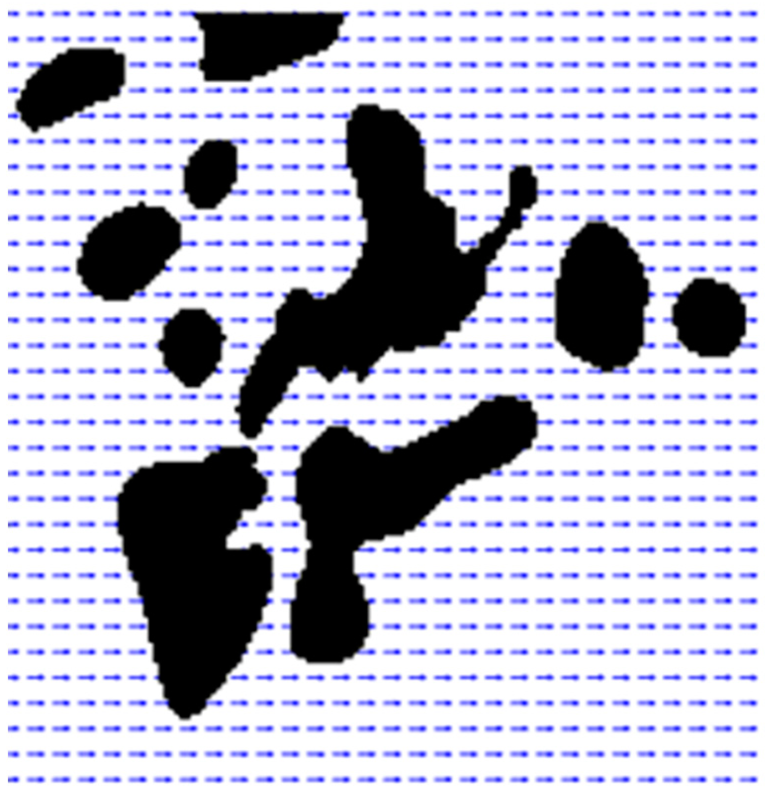
3.1.2. Ocean Current Characteristics

Ocean currents are an important marine environmental factor and significantly influence the behavior of USVs [62]. Therefore, the effect of ocean currents on a USV should be considered when planning its path, and the safe distance between the way and obstacles should be reasonably adjusted according to the currents’ speeds and directions.

Though ocean currents are quite complex in an actual marine environment, for the focus of this research, only steady and horizontal currents were taken into consideration and integrated into the path-planning algorithm for the USV, as exhibited in Figure 2. The ocean current speeds in most of China’s sea areas are between 0 and 1 $\mathrm{k}\mathrm{n}$ [63]. Therefore, currents with speeds of 0.2$\mathrm{k}\mathrm{n}$, 0.6$\mathrm{k}\mathrm{n}$, and 1 $\mathrm{k}\mathrm{n}$ were experimented in this study.

Generally, the generation of currents is modeled with vector fields $J(i,j)$ in a grid map [64]. $U(i,j)$ and $V(i,j)$ are denoted as the velocity component of $J(i,j)$ on the X-axis and Y-axis of the grid map, respectively, and $(i,j)$ are the grid coordinates.

Figure 2. The environmental map under a horizontal current field.

Figure 2. The environmental map under a horizontal current field.

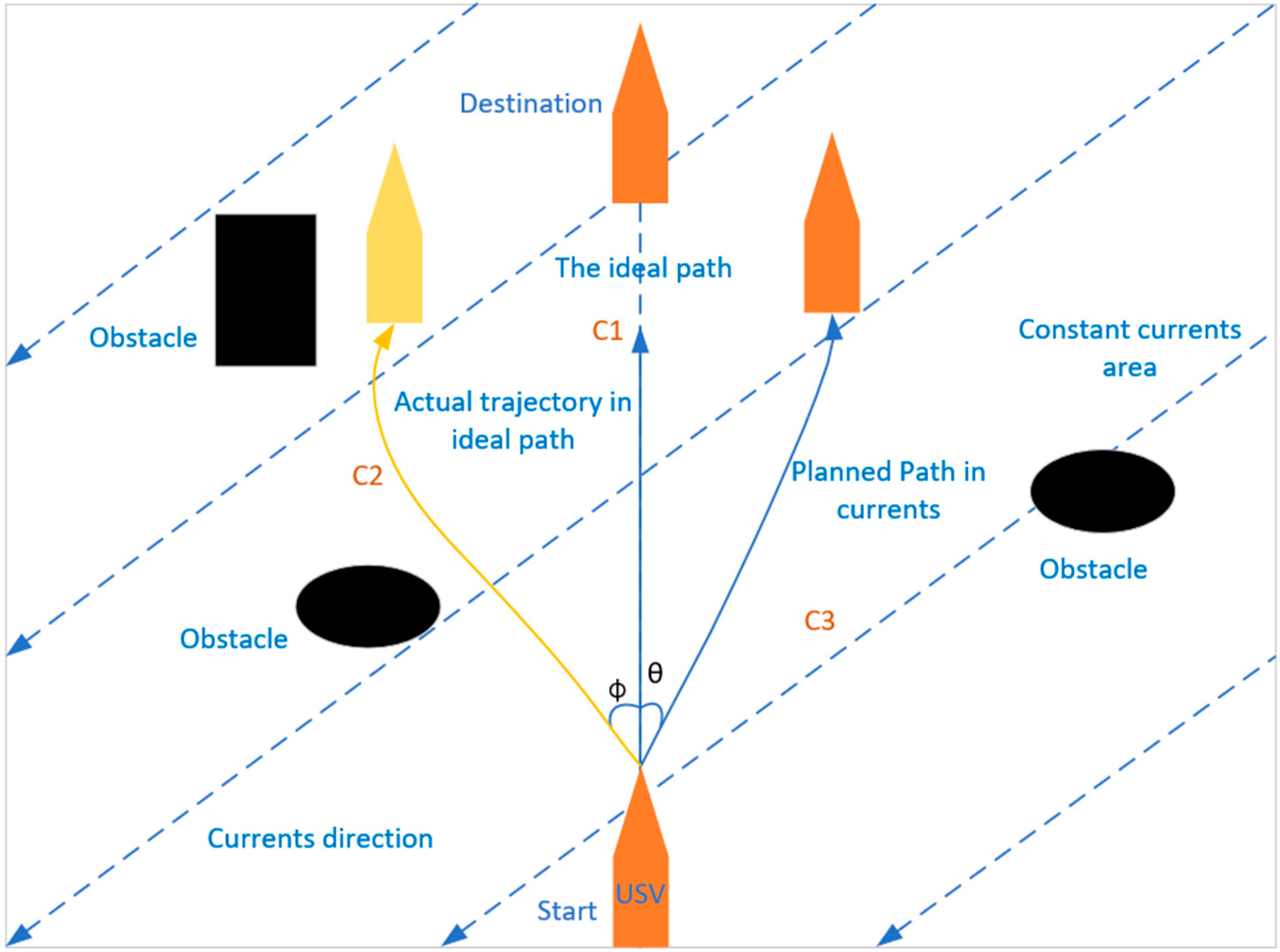
3.1.3. Deviation in the USV Caused by Currents

Ocean currents make it difficult for a USV to follow the preset path smoothly and precisely. For a USV, the effect of ocean currents can be regarded as an external force, which results in deviation and potential collision risks.

To mitigate potential hazards to navigation caused by significant deviations in the distance and bearing between a USV and obstacles in a current environment, it is advisable to establish a predetermined offset value for the impacts of currents on the USV in the path-planning stage. This proactive measure effectively minimizes the likelihood of potential collisions or grounding during actual navigation. As a topic of path planning, this study regarded the USV as a mass point and did not consider the mathematical model of dynamics in its control.

As illustrated in Figure 3, if there are no currents or only very weak currents, the USV will follow path C1 to transit this sea area with many obstacles. However, due to the effect of the southwestward current on the USV, the actual trajectory may deviate from the intended path, C1, resulting in a new path, C2. This will increase the risk of collision between the USV and obstacles on the left side of C2. Contrarily, it would be safer and more advisable to project path C3 for the USV under the effect of the southwestward current.

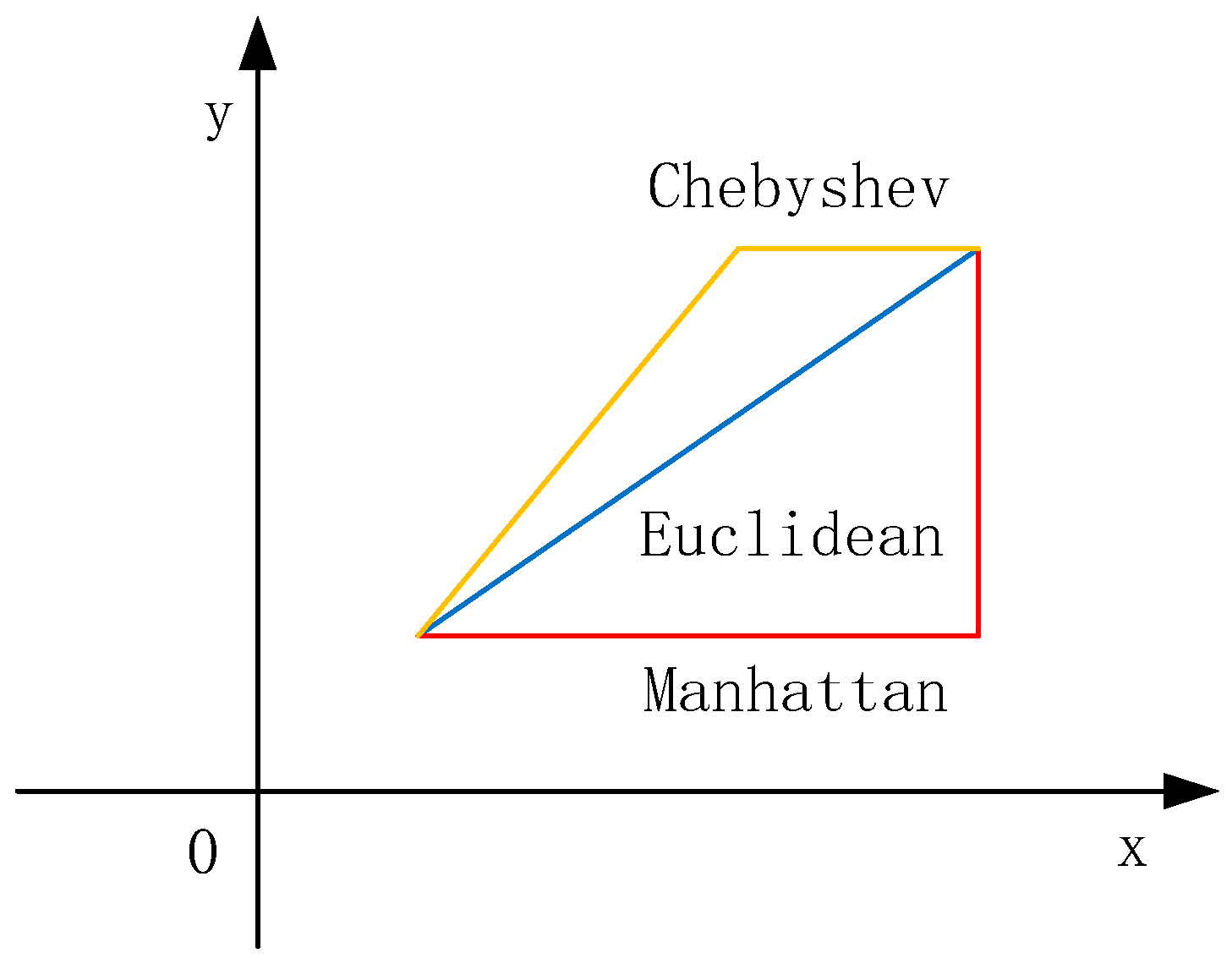
3.2. Traditional A* Algorithm

The A* algorithm is a heuristic path-planning method based on grid maps, which needs to search for path nodes on the environmental map. As demonstrated in Figure 4, the A* algorithm usually performs an extended search for sub-nodes in the grid graph according to the angles of the neighborhood nodes. If the number of neighborhoods is too small, the planned path will not be the shortest, and on the contrary, the steering angle at the turning point will be too small. Therefore, this study searched 8 neighborhoods, and selecting path sub-nodes was more flexible.

Compared with the classic Dijkstra algorithm, a heuristic function was added to guide the search for paths. By defining a cost evaluation function, the A* algorithm can reduce the search range and ensure that the planned path is the shortest. The evaluation function is as follows:

$$f(n)=g(n)+h(n)$$

(5)

where

$n$: The current location node;

$g(n)$: The actual cost from the starting point to the current node;

$h(n)$: The heuristic function, representing the estimated cost from the current node to the target point;

$f(n)$: The total evaluation function, which represents the total cost from the start to the endpoint.

As manifested in Figure 5, according to the different calculation methods of the heuristic function distance, it can be divided into the Euclidean distance, Manhattan distance, and Chebyshev distance. To reduce the turning points of the path, this study chose the Euclidean distance for a relatively short distance and fewer turning times.

Define $\left(x_1, y_1\right)$ and $\left(x_2, y_2\right)$ as the coordinates of two points in the space. The distance $d$ between the two points is calculated by three methods, Euclidean distance, Manhattan distance, and Chebyshev distance, as follows:

$$d_1=\left|x_1-x_2\right|+\left|y_1-y_2\right|$$

(6)

$$d_2=\sqrt{{\left(x_1-x_2\right)}^2+{\left(y_1-y_2\right)}^2}$$

(7)

$$d_3=\left|x_1-x_2\right|+\left|y_1-y_2\right|+(\sqrt{2}-2)\times min\left(\left|x_1-x_2\right|,\left|y_1-y_2\right|\right)$$

(8)

3.3. Improvement of A* Algorithm

The A* algorithm is a heuristic algorithm for solving global path planning in a static environment. It is easy to implement and widely used in path planning. The core idea of the A* algorithm is to calculate the shortest path between the start and endpoints based on the geometric distance without considering the safe distance between the path and obstacles. As a result, the planned path is often close to obstacles. Under the influence of ocean currents, a USV will drift in the direction of the ocean currents, deviating from the expected route. Therefore, when using the A* algorithm to route a USV in a current environment, it needs to be adapted according to the influence of the ocean currents so that the USV can maintain an appropriate safe distance from obstacles.

In this section, the adaption of the A* algorithm includes the elimination of perilous nodes, the introduction of an adaptive guidance angle, and the improvement of the cost function of the algorithm considering the effect of ocean currents.

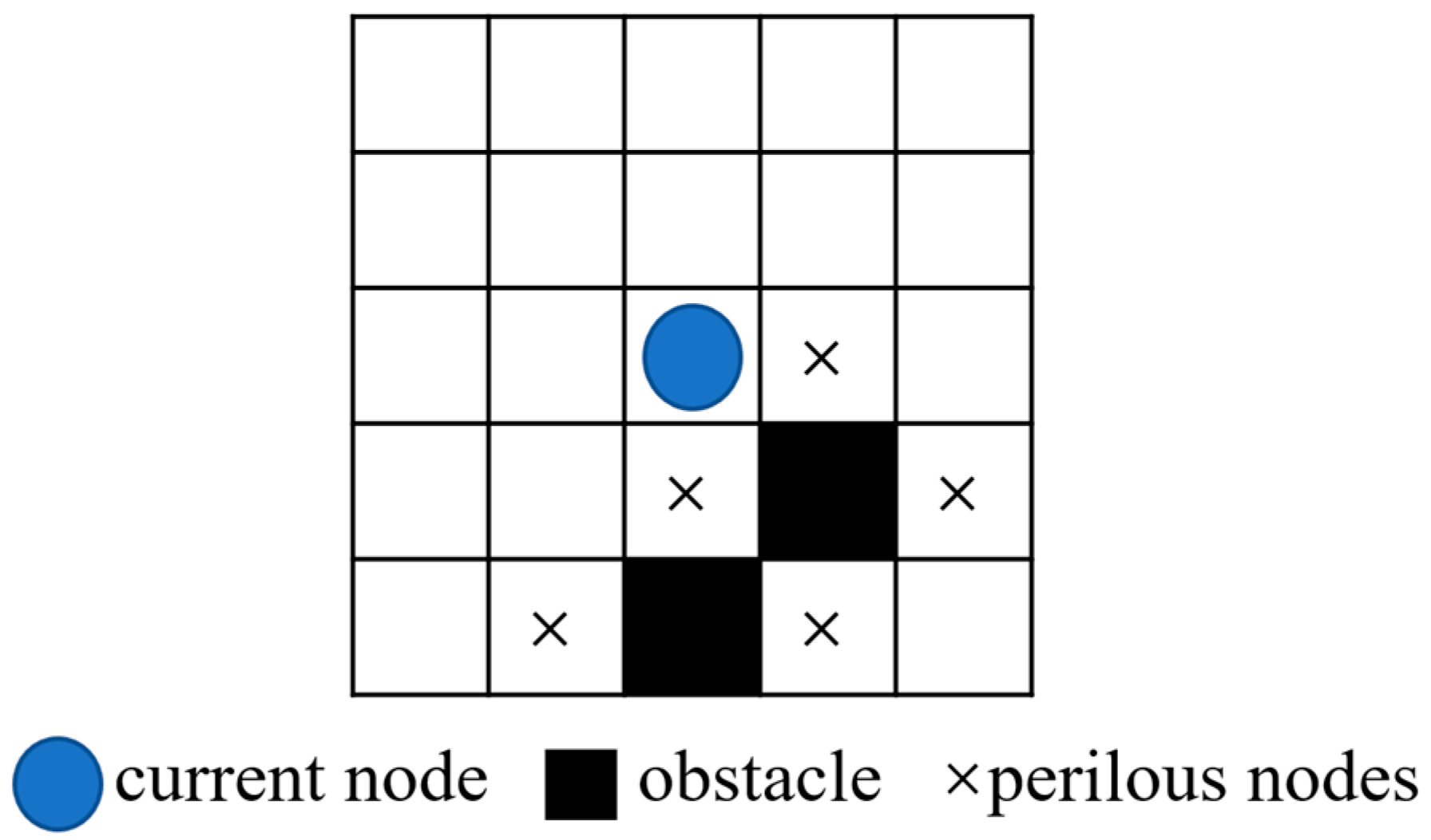
3.3.1. Bypassing Perilous Nodes

In the vicinity of obstacles, the path produced by the A* algorithm will usually pass through the vertices of the obstacles, as shown in Figure 6a,b. In this case, the distance between the USV and obstacles is small and insufficient for safe passing. To increase the safety margin and reduce the potential collision risk during navigation, it is necessary to design the path to avoid the nodes, as illustrated in Figure 6c,d.

To keep the planned path always at a safe distance from obstacles, this paper marked the nodes adjacent to obstacles as perilous nodes, which should be ignored during the search of the A* algorithm. As shown in Figure 7, when obstacles are in the 8 fields of the current node (in blue), the perilous nodes should be marked and ignored first to keep the candidate path well away from the obstacles.

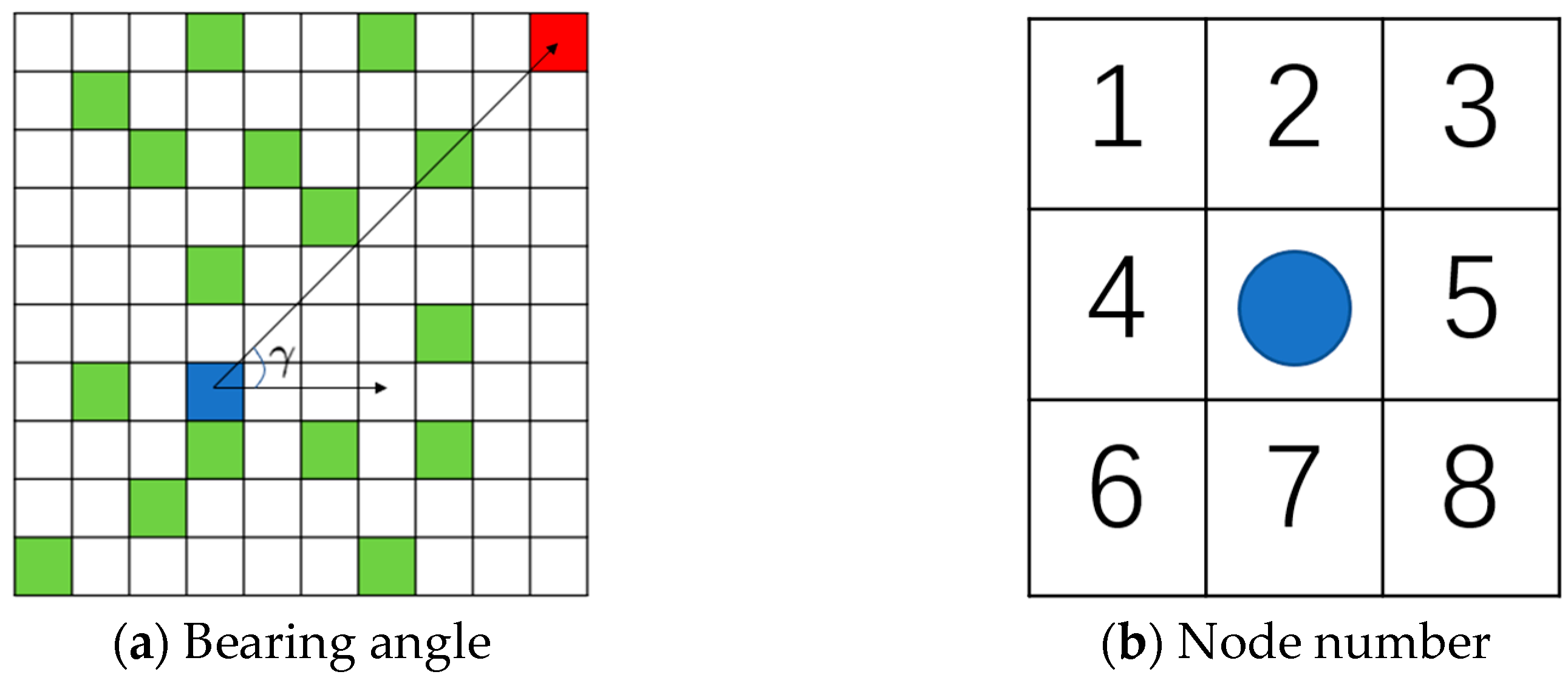
3.3.2. Introduction of Adaptive Guidance Angle

The traditional A* algorithm expands nodes along a fixed 4 or 8 directions, regardless of the direction of the endpoint. However, the nodes along the direction of the endpoint should be processed first for their higher probability of being nodes of the final path. On the contrary, the nodes in the opposite direction to the endpoint should not be processed for the cost function because the final path does not connect these nodes. To reduce the calculation of the cost function, this study introduced the bearing $\gamma$ between the current node and endpoint to distinguish the nodes along or in opposition to the direction of the endpoint. As Equation (9) shows, the bearing $\gamma$ is defined as the angle between the current node and the endpoint:

$$\gamma =\frac{{\tan }^{-1}\left(\frac{y_d - y_n}{x_d - x_n}\right)}{\pi }\cdot 180$$

(9)

where

$\gamma$: The angle between the current node and the endpoint;

$x_d, y_d$: The horizontal and vertical coordinates of the endpoint;

$x_n, y_n$: The horizontal and vertical coordinates of the current node.

The opposite nodes are those three nodes in the 8 neighborhoods of the current node in the opposite direction of the endpoint, as shown in Figure 8 and

Table 1. Bearing corresponds to the opposite node.

Bearing	Opposite Node
(0°~90°)	4, 6, 7
(90°~180°)	5, 7, 8
(180°~270°)	2, 3, 5
(270°~360°)	1, 2, 4

.

As indicated in Figure 8, when planning the path from the blue start point to the red endpoint, the nodes along the endpoint can be preferentially selected for the cost calculation when searching for sub-nodes based on the relationship between the opposite nodes and the bearing in Table 1. If the nodes along the endpoint are obstacles (green grids) or perilous, then those opposite nodes are processed first for the cost calculation. According to the principle discussed, the processing order would be nodes 3, 2, 5, 1, 8, 4, and 7.

3.3.3. Improvement of the Cost Function with an APF

When a USV sails in the water, ocean currents with different directions and speeds will act on the USV and change the distance between the USV and obstacles. Ocean currents increase the difficulty for a USV to precisely follow a preset path. If ocean currents push the USV toward an obstacle, there will be a risk of collision between the USV and the obstacle or grounding. To tackle this risk of collision and grounding, this study considered the effects of ocean currents on USVs. It adjusted the distance between the USV and obstacles according to the various conditions of ocean currents. If ocean currents flow toward the obstacle, the distance increases accordingly and vice versa.

As indicated in Figure 9, path S1 transits through the sea area with equal distance to both side obstacles if there are no currents. If there are easterly currents in this sea area and the USV follows path S1, it will be pushed by currents toward the downstream obstacles. Therefore, it is necessary to increase the safe distance $d$ to $D$, and path S2 is generated according to the conditions of the ocean currents, as displayed in Figure 9. Expanding distance $D$ will decrease the difficulty of USV navigation control and the risk of collision with obstacles.

To set an appropriate safe distance $D$ as discussed above, this study integrated an APF into the A* algorithm to embody the influence of currents on the safe distance between the USV and obstacles. Thus, the USV can stay away from the obstacle area and remain at an appropriate safe distance during navigation.

An APF is an algorithm applied in local path planning, drawing on the potential field concept in physics. Ocean currents will exert a force on a USV during its voyage, so the effect of the currents can be considered equivalent to the potential field force exerted by obstacles, which is composed of attraction and repulsion. When the USV is pushed toward obstacles by the currents, it will be subjected to the repulsive force from obstacles, which can attenuate the force of the currents. Conversely, if the currents pull the USV away from obstacles, it will be subjected to the attractive force from obstacles. The improved total cost function of Formula (5) was revised in Formula (10):

$$f(n)=g(n)+h(n)+\omega m(n)$$

(10)

$$\left\{\begin{array}{l}m(n)=\left\{\begin{array}{c}{F}_1, c=-1\\ F_2, c=1\end{array}\right.\\ F_1=\epsilon \rho \left(q, q_{obs}\right)\\ F_2=k\left(\frac{1}{\rho \left(q, q_{obs}\right)}-\frac{1}{{\rho }_d}\right)\frac{1}{\rho \left(q, q_{obs}\right)}\end{array}\right.$$

(11)

where

$m(n)$: The potential field force;

$F_1$,${ F}_2$: The attractive and repulsive forces of the obstacles;

$\epsilon , k$: The proportional gain coefficient;

$\rho \left(q,q_{obs}\right)$: The distance between the current node and obstacles, $0<\rho \left(q,q_{obs}\right)<{\rho }_d$;

$\omega$: The weight coefficient of the potential field force;

$c$: The values of ‘−1’ and 1 represent the obstacles’ attractive and repulsive forces on the USV, respectively. When the USV is pushed toward obstacles, the value of $c$ is set as 1. Conversely, if the USV is pulled away from obstacles, the value of $c$ is set as ‘−1’;

${\rho }_d$: The maximum acting distance of obstacles on the USV in an ocean current environment, which will be discussed more in the following section.

The dimensions of the attractive and repulsive forces are different from those of the distance in the same formula. Therefore, it is necessary to equate the dimension of the force to that of the distance by adjusting the value of $\omega$.

To illustrate the path planning with the proposed A* algorithm under the influence of currents, the selection of path nodes for different currents is exhibited in Figure 10 and analyzed accordingly.

Figure 10 shows two types of marine environments with reciprocal ocean currents. For the USV, the left-side current is in-obstacle, which pushes the USV toward obstacles, and the right-side current is off-obstacle, which pulls the USV away from obstacles. To attenuate these effects of currents on the USV and keep a proper safe distance, the improved A* algorithm in this study used an attractive force $F_1$ and a repulsive force $F_2$ on the USV to reflect the impact of currents. Forces $F_1$ and $F_2$ are proportional to the magnitude of currents, which are embodied in the cost function Formulas (10) and (11). Under the conditions of in-obstacle currents, the improved A* algorithm connects the orange nodes (rather than the red nodes) to produce a path to meet the requirement of the threshold value of the safe distance $d_{\mathrm{safe} }$.

3.3.4. Maximum Acting Distance of Obstacles with Currents

As analyzed in the above section, the maximum acting distance ${\rho }_d$ of the potential field force is generated by obstacles on the USV in a current environment. The ${\rho }_d$ plays a very important role in path planning for a USV in an ocean current environment. From the discussions in Section 3.1.3 and Section 3.3.3, we can find that the maximum acting distance ${\rho }_d$ is a non-linear function of several variables, such as the speed and direction of currents, the speed and size of the USV, the angle between the heading of the USV and currents, and so on. Owing to the intricacy of this non-linear function, the determination of this non-linear function was beyond the scope of this study. To simplify the calculation of ${\rho }_d$ and consider the fact that the ${\rho }_d$ is greatly and mainly affected by currents, this paper assumes that the aforementioned non-linear function is degraded to a linear function of the current speed and length of the USV, as shown in Equation (12). The ${\rho }_d$ increases proportionally with the speed of the current and the length of the USV.

$${\rho }_d=\alpha v+\beta L$$

(12)

where

$\nu$: The current speed;

$L$: The length of the USV;

$\alpha , \beta$: The respective coefficients of $\nu$ and $L$;

$\alpha$ and $\beta$ are determined through a series of experiments with the specific particulars of the currents and the USV.

As exhibited in Equation (12), the maximum acting distance ${\rho }_d$ includes two parts, which reflect the effects of the ocean currents and the size of the USV. If there are no currents, the ${\rho }_d$ only considers the size of the USV, as shown in the second part of the Equation (12).

For the complexity of the movement of USVs in an ocean environment with currents, the angles between the heading of the USVs, the directions of currents, and obstacles are ignored in the path-planning stage. Whatever angles are between them, the effects of currents on USVs and path planning greatly vary. As a result, the first part of the ${\rho }_d$ only considers the magnitude of the current speed.

3.3.5. Bezier Curve Smoothing

The path generated by the A* algorithm is a connection between nodes without regarding the smoothness of the path, which should be controllable in real time and intuitive for the navigation and control of the USV automatically. This study adopted the Bezier curve for path smoothing because of its easy implementation and good performance. The number of its control points determines the smoothness of the Bezier curve. When the number of control points is $n+1$, the Bezier curve parameter equation of its n-degree polynomial can be obtained [65].

$$\left\{\begin{array}{l}P(t)={\displaystyle \sum _{i=0}^n} P_i{B}_{i,n}(t), t\in [0, 1]\\ B_{i,n}(t)=C_n^i{t}^i(1-t{)}^{n-i}, i=0, 1, 2, \cdots , n\end{array}\right.$$

(13)

where

$P(t)$: The coordinates of control points;

$B_{i,n}(t)$: The basic functions for the Bezier curve;

$t$: The intermediate variables during normalization;

$n$: The Bezier curve optimization times.

As shown in Figure 11, points A, B, and C are three path points on the polyline segment, equivalent to three control points on the second-order Bezier curve. Firstly, two points, M and N, are taken according to the proportional relationship between the line segment AB and BC and they are connected, and then point P on the line segment MN is taken according to the same proportional relationship, so that it satisfies the following proportional relationship: $\mathrm{A}\mathrm{M}/\mathrm{A}\mathrm{B}=\mathrm{B}\mathrm{N}/\mathrm{B}\mathrm{C}=\mathrm{M}\mathrm{P}/\mathrm{M}\mathrm{N}$. P is one of the points on the second-order Bezier curve. APC is a segment of the path that is to be smoothed. By this method, the path is smoothed by connecting all segments.

3.3.6. The Pseudocode and Flowchart of Improved A* Algorithm

The improved A* algorithm eliminates perilous nodes by expanding 8 neighborhood nodes and adaptive guidance angles. Then, the values $m(n)$, $g(n)$, $h(n)$, and $f(n)$ of each node are calculated according to the directions and speeds of currents. The nodes with their function values are put into the Openlist. The nodes with the minimum value $f(n)$ calculated each time are deposited into the Closelist. All nodes with the minimum value $f(n)$ form the initial path, which is smoothed to obtain the final path, as discussed in Section 3.3.5. The pseudocode of Algorithm 1 and flowchart of improved A* algorithm is shown below and in Figure 12.

Algorithm 1: Improved A*

Input: start node, goal node, map, currents parameter Output: smoothed path 1: Openlist = [], Closelist = [], path = [], distance = []; 2: Mark N[start] as Openlist; 3: Set $k$, $\omega$, $c$, ${\rho }_d$, currents speeds; 4: While Openlist ≠ Ø do 5:  Search neighbor nodes of N[i] in Openlist parent node; 6:  for child node in neighbor nodes 7:    If child node = obstacle, perilous node or in the direction of N[goal] 8:      child node = null; 9:    else 10:     child nodes = child node; 11:     calculate $g_n[\mathrm{i}]$, $h_n[\mathrm{i}]$, $m_n[\mathrm{i}]$, $f_n[\mathrm{i}]$ of child nodes; 12:     select min ($f_n[\mathrm{i}]$) in child nodes as Openlist N[i]; 13:     if N[i] = N[goal] then 14:       return “path is found” and smooth the path; 15:     else 16:       Mark N[i] as Closelist; 17:       if successor Ni[j] of N[i] not in Closelist or Openlist then 18:         Mark Ni[j] as Openlist; 19:         calculate $g_n[\mathrm{i}]$, $h_n[\mathrm{i}]$, $m_n[\mathrm{i}]$, and $f_n[\mathrm{i}]$, respectively; 20:         if Ni[j] in Openlist and $f$(Ni[j]) is smaller than $f$(Nm[j]) then 21:           f(Nm[j]) = f(Ni[j]) and set parent node of N[j] as N[i] 22:         end if 23:       end if 24:     end if 25:   end if 26:  end for 27: end while 28: return “path is not found”.

4. Experiments and Numerical Analysis

In this section, a series of simulations performed on two different maps to evaluate the effectiveness of the proposed path-planning algorithm by the improved A* algorithm were detailed. The experiment in Section 4.1 simulated a marine environment without currents, and that in Section 4.2 was with various currents. All experiments were coded in MATLAB 2016a and run on a computer with Windows 10, an Intel i5-7200U 2.71 GHz processor, and 16 GB of RAM. The grid and currents in the visualization state easily cause visual interference, so this paper hid the grid in the figure.

4.1. Path Planning without Currents

In this section, the experiments carried out with the path-planning algorithms of the original A*, APF, RRT, PSO, and the proposed A* are presented to compare and verify the effectiveness of the improvements (Section 3.3.1 and Section 3.3.2) of the proposed A* algorithm.

In all experiments detailed in this section, the size of the USV was set to 5 m in length by 3 m in width. The actual size of the sea area map was 6000 m × 6000 m and designed to be a 150 × 150 grid with each side of 40 m. Generally, the safe distance $d_{\mathrm{safe} }$ was set to be 40 m. Furthermore, the ocean currents were not considered in the experiments in this section.

4.1.1. Simulation Experiment 1 and Result Analysis

The task of path planning was to program a path from the starting point (125, 25) to the target point (10, 140). The paths obtained by different algorithms are manifested in Figure 13, and the performance is shown in

Table 2. Comparison with different algorithms in simulation 1.

Algorithms	Path Length/m	Min. Distance to Obstacle/m	Running Time/s	Turning Points
Original A*	7325.2	0	9.1	16
APF	7341.2	44.2	19.2	7
PSO	7570.6	0	41.6	2
RRT	9553.2	252.6	13.8	28
Improved A*	7442.4	141.4	7.8	13

.

Based on Figure 13 and Table 2, the improved A* algorithm performed best in the minimum distance to obstacles and running time, obtaining 141 m and 7.8 s, respectively. Compared with the original A*, there was a 14.3% improvement in the running time for the improved A* and fewer turning points. As discussed in Section 3.3, eliminating perilous nodes and following the adaptive guidance angle resulted in this advancement in the running time and minimum distance.

Although the length of the paths planned by the original A* and the APF was shorter than that planned by the improved A*, and the minimum distances to obstacles and running time were inferior to those obtained by the proposed A* algorithm. Significantly, the minimum distances to obstacles from paths obtained by the original A*, APF, and PSO were less than or close to the preset safe distance (40 m), which made the paths unacceptable.

4.1.2. Simulation Experiment 2 and Result Analysis

In these experiments, the environment with relatively few obstacles and ocean currents was preset, and the paths from the starting point (125, 30) to the target point (20, 140) were planned by different algorithms. The simulation results are shown in Figure 14, and the simulation data are shown in

Table 3. Comparison with different algorithms in simulation 2.

Algorithm	Path Length/m	Min. Distance to Obstacle/m	Running Time/s	Turning Points
Original A*	6512.8	0	6.7	13
APF	-	-	-	-
PSO	6624.8	44.8	8.5	3
RRT	9040.8	204.8	5.3	22
Improved A*	6724.4	136.4	4.8	8

Note: ‘-’ indicates that the algorithm failed to plan a complete path in this case.

.

Similar to the experiments in Section 4.1.1, the improved A* algorithm in this study surpassed the other algorithms in the running time and minimum distance to obstacles and showed relative weakness in the length and turning points of the path planned. The improved A* algorithm’s turning points were less than those of the original A*. Because there was no space between the path obtained and the obstacle, the path produced by the original A* was invalid.

In conclusion, the paths planned by the original A* and PSO algorithms were close to the obstacles and failed to maintain a safe distance. At the same time, the paths planned by the RRT algorithm had a large number of turning points and a longer length. In contrast, the path planned by the improved A* algorithm performed better overall than the others.

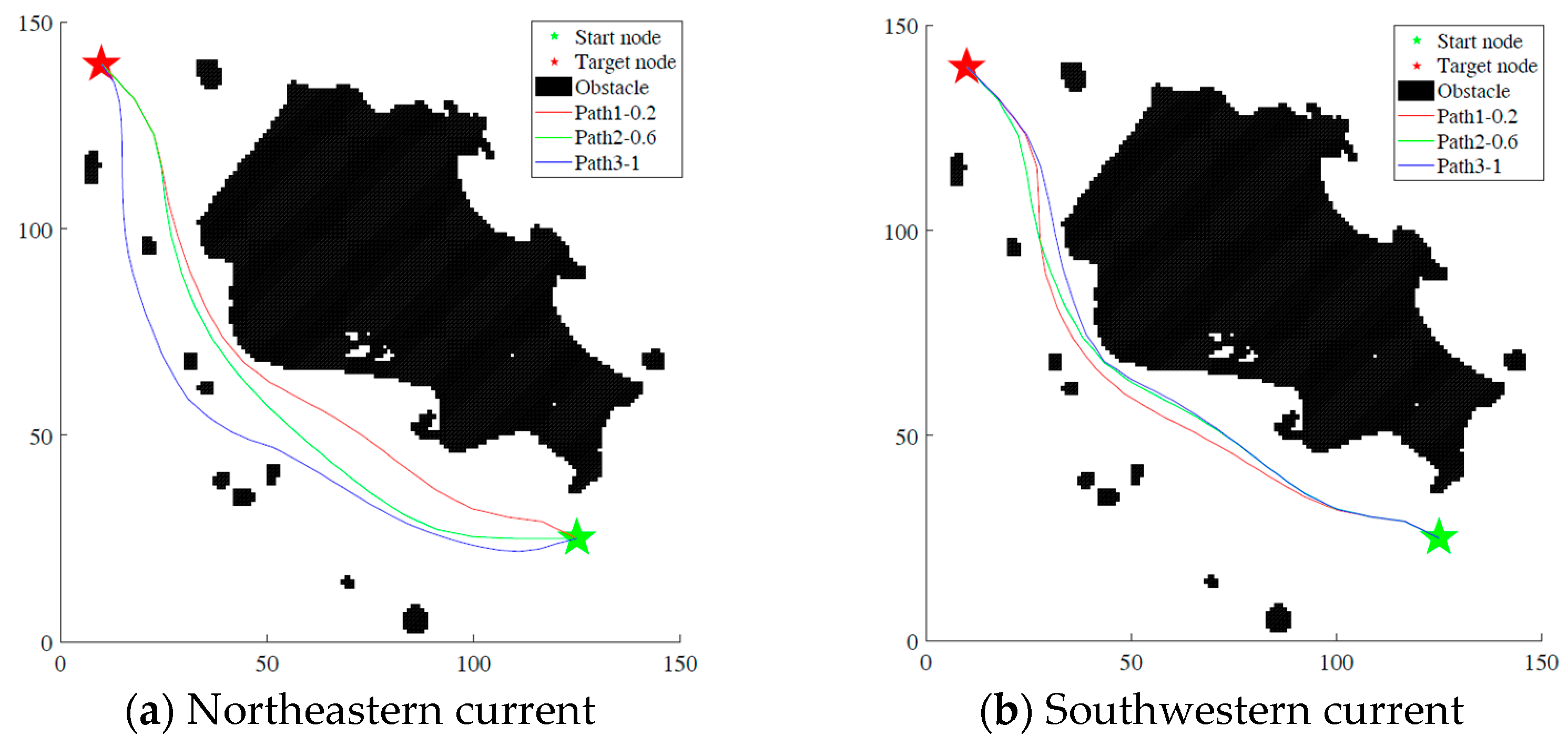
4.2. Path Planning under Different Ocean Current Conditions

In the experiments in this section, we constructed two grid maps in combination with northeastern and southwestern currents with varying speeds to verify the performance of the improved A* under the influence of various ocean currents. Furthermore, to explore the influence of different currents on path planning for the USV, three current speeds were used to represent the various current conditions. Specifically, the current strengths were represented by weak currents (0.2 $\mathrm{k}\mathrm{n}$), moderate currents (0.6$\mathrm{k}\mathrm{n}$), and strong currents (1$\mathrm{k}\mathrm{n}$). There were six situations of ocean currents with three speeds (0.2$\mathrm{k}\mathrm{n}$, 0.6$\mathrm{k}\mathrm{n}$, and 1$\mathrm{k}\mathrm{n}$) and two directions (northeast and southwest).

For the specific particulars of the currents and USV in these experiments, through trial and error, the coefficients $\alpha$ and $\beta$ for Formula (12) were determined. The function of ${\rho }_d$ in Formula (13) is instantiated as follows:

$${\rho }_d=100v+20L$$

(14)

According to Formula (13), the maximum influence distances ${\rho }_d$ of obstacles acting on the USV with a length of 5 m were set to 120 m, 160 m, and 200 m for the three ocean currents speeds (0.2 $\mathrm{k}\mathrm{n}$, 0.6$\mathrm{k}\mathrm{n}$, and 1$\mathrm{k}\mathrm{n}$), respectively.

Furthermore, through trial and error, the basic parameters of the algorithms were set as the gain coefficients $\epsilon =0.3$, $k=0.7$, the safety radius $R=10 \mathrm{m}$, and the safe distance $d_{\mathrm{safe} }=60 \mathrm{m}$. The weighting coefficient $\omega$ was set to 0.2.

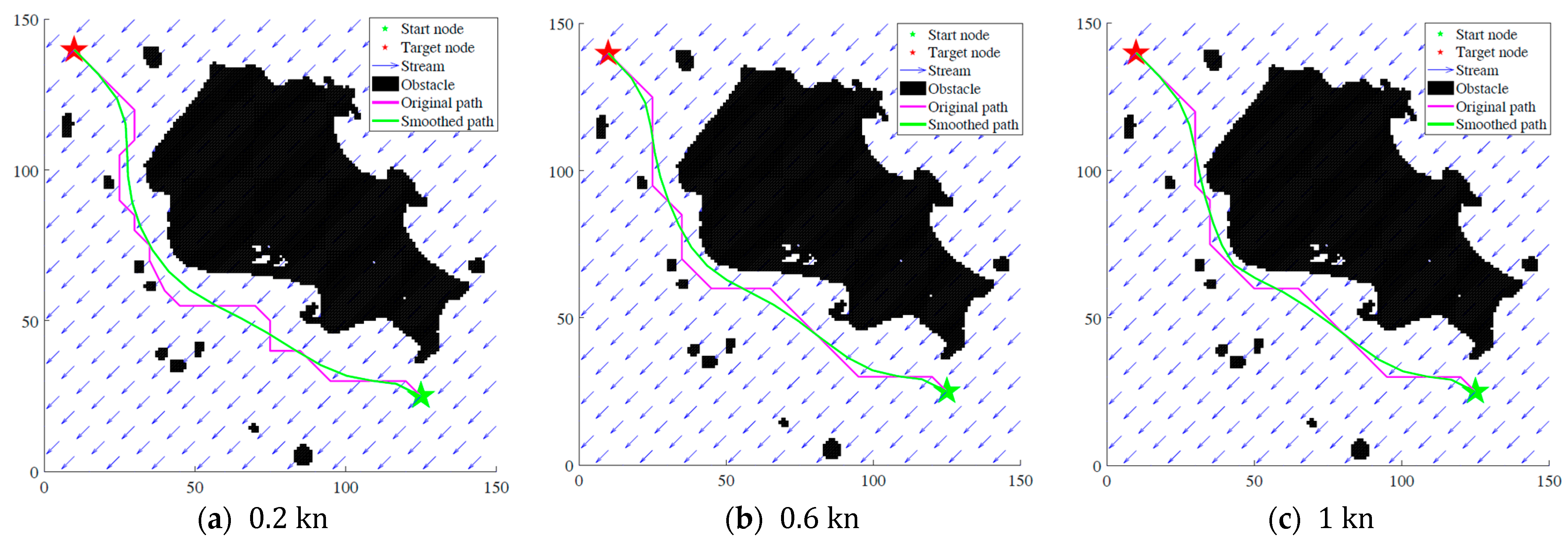
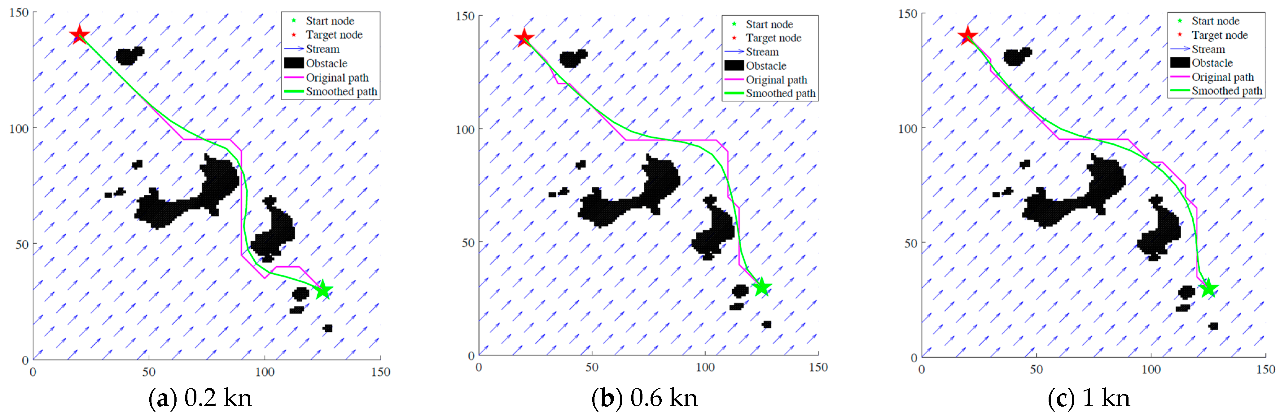
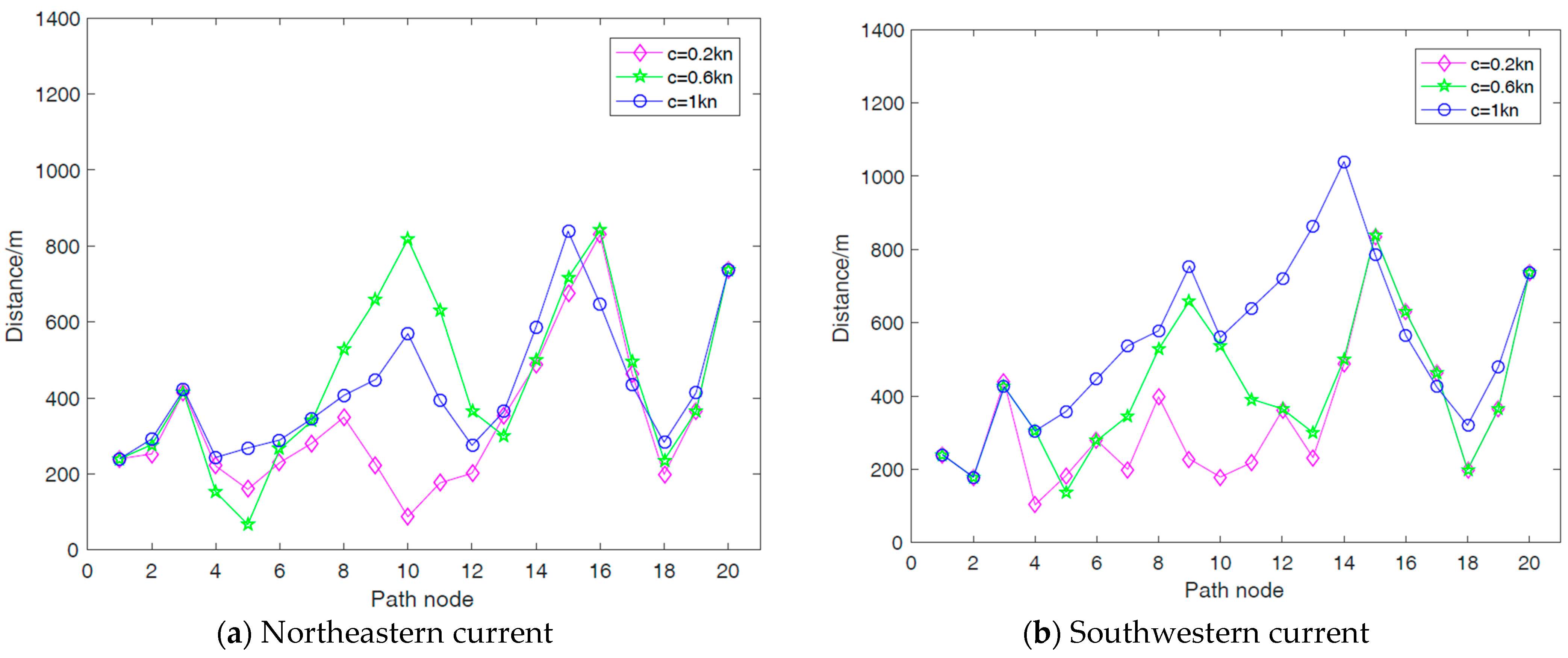
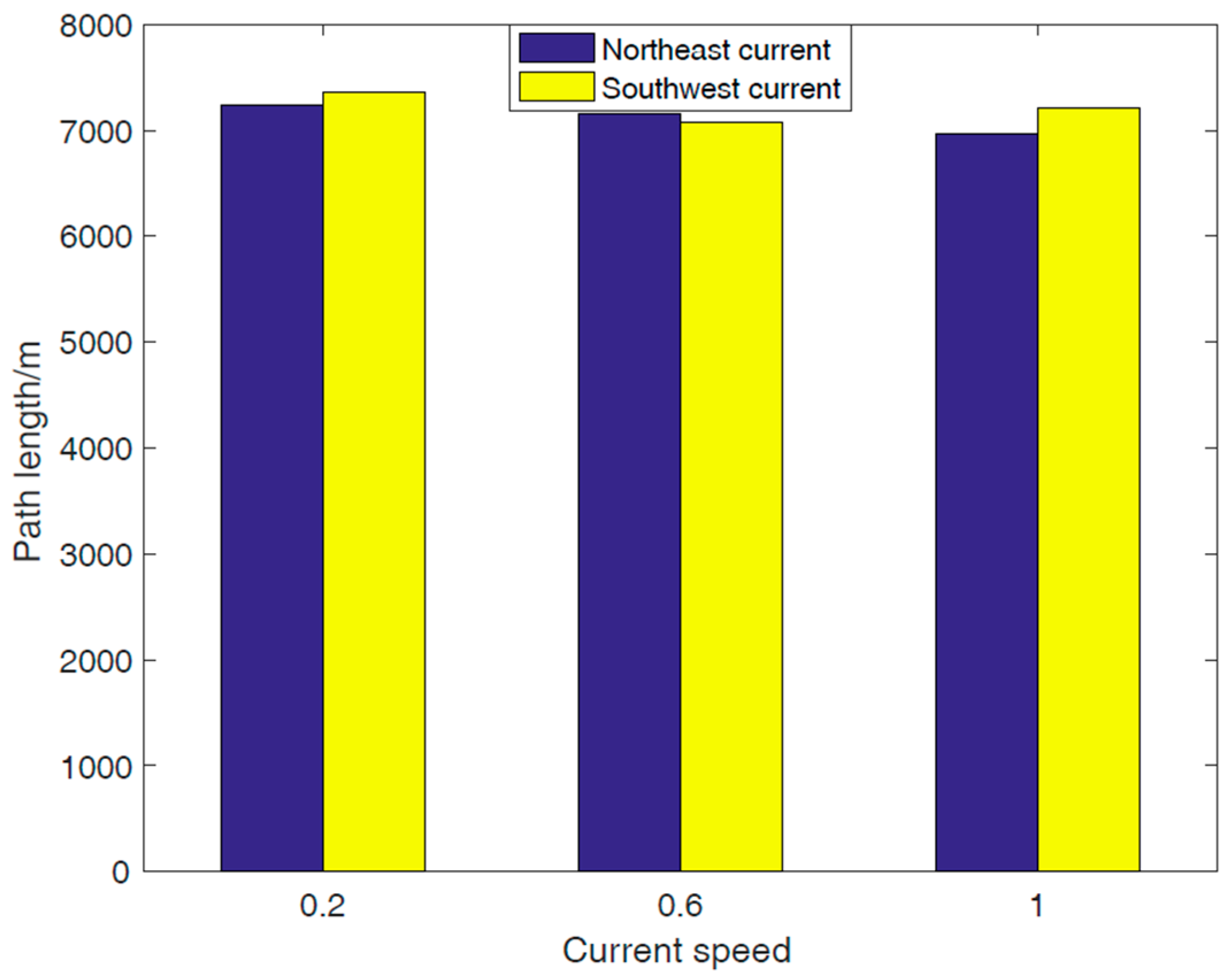
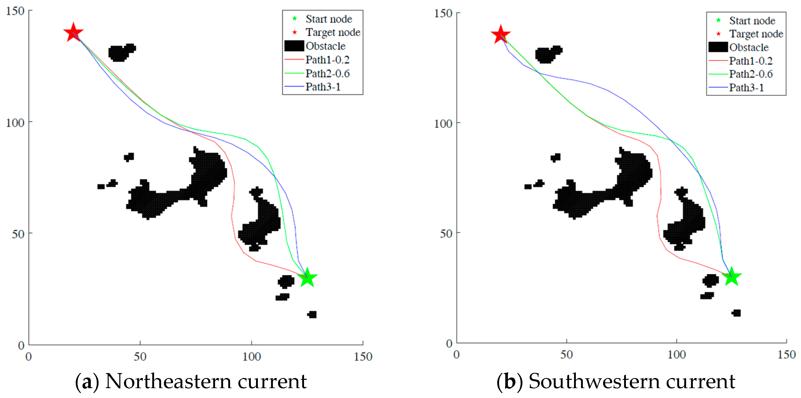
4.2.1. Simulation Experiment 3 and Result Analysis

The starting point was set to (125, 25), and the target point was set to (10, 140). The results of the simulation experiments are shown in Figure 15, Figure 16, Figure 17, Figure 18 and Figure 19 and

Table 4. Simulation results of northeastern currents in simulation 3.

Current Speed/$\mathbf{k}\mathbf{n}$	Path Length/m	Shortest Distance/m	Running Time/s
0.2	7559.6	62.4	17.6
0.6	7559.6	152.6	15.6
1	8359.6	116.8	13.5

and

Table 5. Simulation results of southwestern currents in simulation 3.

Current Speed/$\mathbf{k}\mathbf{n}$	Path Length/m	Shortest Distance/m	Running Time/s
0.2	8040.2	184.6	15.2
0.6	7559.6	104.8	14.5
1	7442.4	72.4	16.8

under the influences of different ocean currents. The experimental results and analysis are as follows.

As discussed in Section 3.3.3, the forces of currents acting on the USV will push the USV away from the preset track, which brings about the potential risk of collision with obstacles or grounding in shallow water.

Figure 15. Improved A* paths with different speeds of northeastern currents in simulation 3.

Figure 15. Improved A* paths with different speeds of northeastern currents in simulation 3.

Figure 16. Improved A* paths with different speeds of southwestern currents in simulation 3.

Figure 16. Improved A* paths with different speeds of southwestern currents in simulation 3.

The improved A* algorithm automatically adjusts the distance to obstacles according to the different ocean current conditions. As displayed in Figure 15, the northeastern currents will push the USV toward the big obstacle (the island). To counteract this effect of the currents, the improved A* algorithm gradually increases the distance to the obstacle in line with the increasing speed of the currents. The closest smoothed path–obstacle distances were 62.4 m, 152.6 m, and 116.8 m, for current speeds of $0.2 \mathrm{k}\mathrm{n}$, $0.6 \mathrm{k}\mathrm{n}$, and $1 \mathrm{k}\mathrm{n}$, respectively, as manifested in Table 4. Moreover, these distances still maintained a sufficient safe distance of 60 m. To observe the changes in the path–obstacle distance, 20 path points on the smoothed path were sampled, and the path–obstacle distances were recorded as indicated in Figure 16, which reflected the trend of the distance change in line with the speed of the currents.

Furthermore, due to the limited sea room, strong northeastern currents ($1 \mathrm{k}\mathrm{n}$) made it impractical and unsafe for the USV to transit between the obstacles, as shown in Figure 15c. In this case, the path obtained bypassed the narrow sea channel and passed far southwards of the islands. Accordingly, the length of the path increased to 8359.6 m.

In southwestern currents, Table 5 and Figure 16 show that the improved A* algorithm also planned a collision-free smoothed path from the starting point to the endpoint for the USV with currents speeds of $0.2 \mathrm{k}\mathrm{n}$, $0.6 \mathrm{k}\mathrm{n}$, and $1 \mathrm{k}\mathrm{n}$. As the southwestern currents will push the USV southwestwards away from the big obstacle (the island), the path could be close to the big obstacle to shorten the length of the path. On the contrary to the situations with northeastern currents, the distances to obstacles decreased, which were inversely proportional to the speed of currents, as stated in Table 4 and Figure 15, Figure 16 and Figure 17. The smoothed shortest distances decreased from 184.6 m to 72.4 m for the southwestern current with speeds of $0.2 \mathrm{k}\mathrm{n}$, $0.6 \mathrm{k}\mathrm{n}$, and $1 \mathrm{k}\mathrm{n}$. Accordingly, the length of the path decreased to 7442.4 m.

Figure 17. The shortest path–obstacle distance in simulation 3.

Figure 17. The shortest path–obstacle distance in simulation 3.

Figure 18 shows that the overall length of paths changes mildly in different current situations. However, the running time of algorithms in different cases of currents slightly increased, which was inversely proportional to the length path, as manifested in Table 4 and Table 5. Additionally, Figure 19 shows that the improved A* algorithm can effectively produce appropriate and smooth paths according to various ocean currents, which meet the requirements of the safe navigation of the USV.

Figure 18. Comparison of path length vs. various ocean currents in simulation 3.

Figure 18. Comparison of path length vs. various ocean currents in simulation 3.

Figure 19. Comparison of paths vs. various ocean currents in simulation 3.

Figure 19. Comparison of paths vs. various ocean currents in simulation 3.

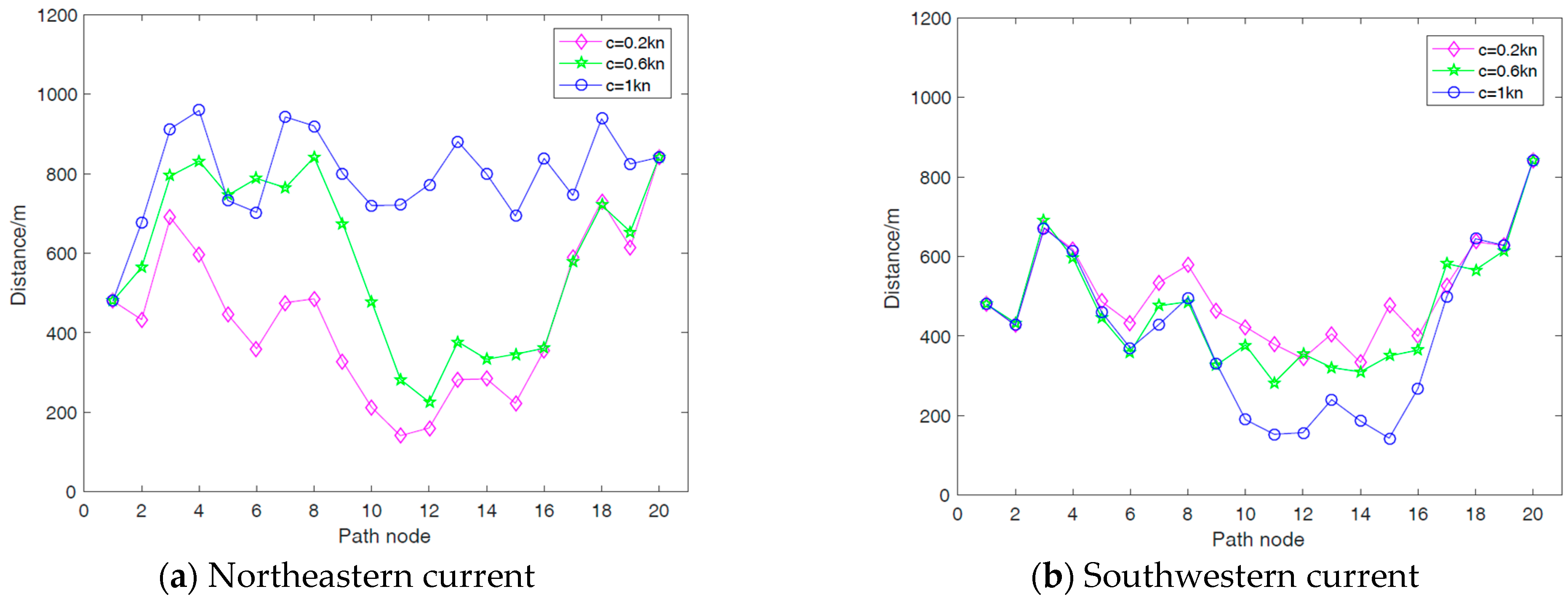
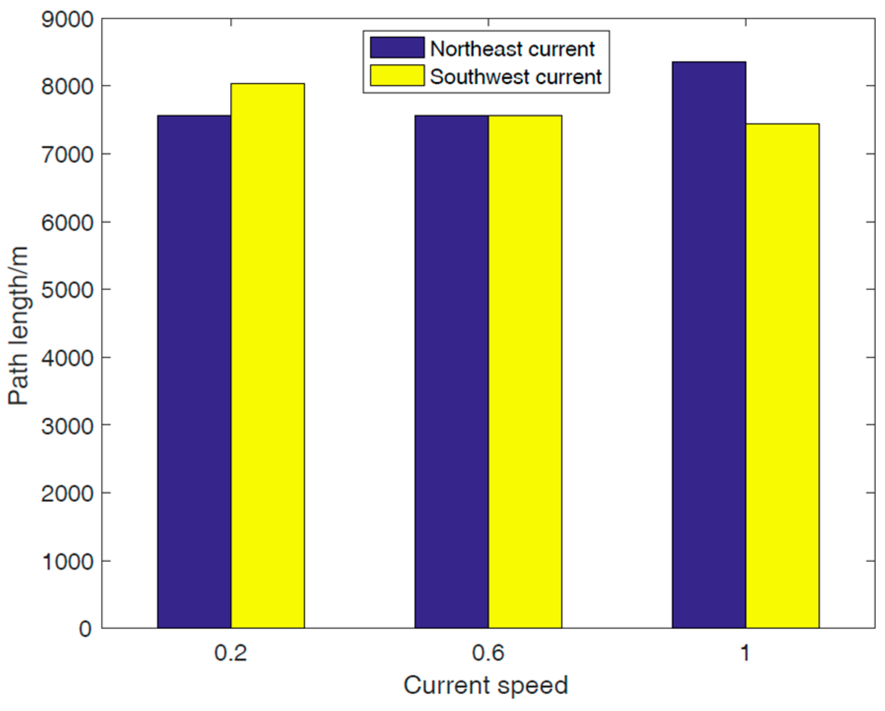
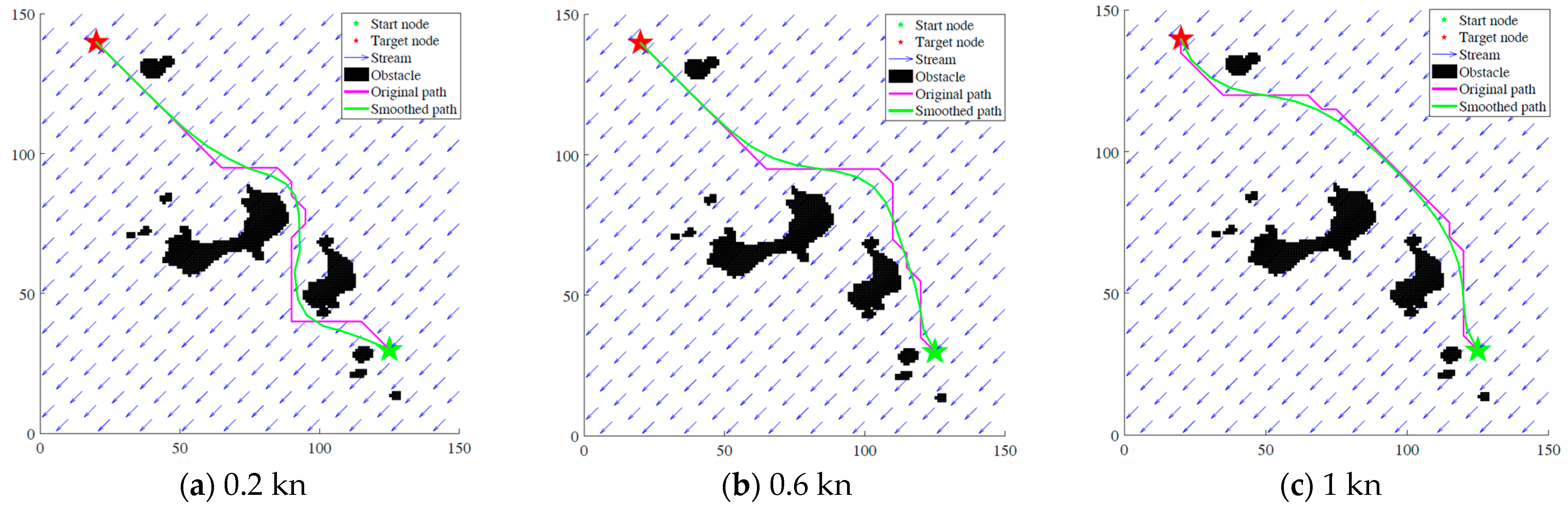
4.2.2. Simulation Experiment 4 and Result Analysis

To further verify the effectiveness of the improved A* algorithm, another marine environment with different obstacles was established to conduct experiments. As demonstrated in Figure 20 and Figure 21, the planning task was to program a path from the starting point (125, 30) to the target point (20, 140) in the ocean currents with northeast and southwest directions and speeds of $0.2 \mathrm{k}\mathrm{n}$,$0.6 \mathrm{k}\mathrm{n}$, and $1 \mathrm{k}\mathrm{n}$.

The results of the simulation experiments are shown in Figure 20, Figure 21, Figure 22, Figure 23 and Figure 24 and

Table 6. Simulation results of northeastern currents in simulation 4.

Current Speed/$\mathbf{k}\mathbf{n}$	Path Length/m	Shortest Distance/m	Running Time/s
0.2	7142.4	65.6	4.8
0.6	7158.2	88.2	4.9
1	6959.6	184.8	4.7

and

Table 7. Simulation results of southwestern currents in simulation 4.

Current Speed/$\mathrm{kn}$	Path Length/m	Shortest Distance/m	Running Time/s
0.2	7158.6	62.2	4.7
0.6	7076.8	148.2	5.4
1	7206.8	183.8	4.8

under the influence of different ocean currents. As manifested in Table 6, the closest smoothed path–obstacle distances were 65.6 m, 88.2 m, and 184.8 m, respectively, which maintained a sufficient safe distance of 60 m. The length of paths decreased from 7158.2 m to 6959.6 m.

Figure 20. Improved A* paths with different speeds of northeastern currents in simulation 4.

Figure 20. Improved A* paths with different speeds of northeastern currents in simulation 4.

Figure 21. Improved A* paths with different speeds of southwestern currents in simulation 4.

Figure 21. Improved A* paths with different speeds of southwestern currents in simulation 4.

Meanwhile, 20 path points on the smoothed path were sampled, and the path–obstacle distances were recorded as indicated in Figure 22, which reflected the trend of the distance change in line with the speed of currents. Similar to the situations in Section 4.2.1, the improved A* algorithm successfully designed the path among many obstacles (islands and isles) by adjusting the path–obstacle distances according to the different situations of ocean currents. As displayed in Figure 20 and Figure 21, for the low current speed ($0.2 \mathrm{k}\mathrm{n}$), the paths transited narrow channels between two bigger islands, though the path length was not the shortest. However, the improved A* algorithm designed the paths to avoid this narrow channel and go further northeastward to keep appropriate path–obstacle distances. Regardless of whether the currents were northeastern or southwestern, the smoothed shortest path–obstacle distances improved in line with the increasing current speed, as revealed in Table 6 and Table 7.

Figure 22. The shortest path–obstacle distance in simulation 4.

Figure 22. The shortest path–obstacle distance in simulation 4.

Figure 23. Comparison of path length vs. various ocean currents in simulation 4.

Figure 23. Comparison of path length vs. various ocean currents in simulation 4.

Figure 24. Comparison of paths vs. various ocean currents in simulation 4.

Figure 24. Comparison of paths vs. various ocean currents in simulation 4.

Figure 23 and Table 6 and Table 7 showed that the overall length of paths and the running time of algorithms mildly changed in different situations of currents. For better analysis and a clearer view, all paths were smoothed by the method discussed in Section 3.3.4 and integrated as shown in Figure 24. Depending on the current direction, six paths with different colors could still be obtained for the three set current velocities. Therefore, the above four sets of experiments have proved the effectiveness of the improved A* algorithm proposed in this article. It can plan different safe paths based on the flow speed and direction while ensuring a safe distance between the USV and obstacles.

In summary, under the action of the heuristic function in the A* algorithm, the distances of the paths from the obstacles are different for different current directions and flow velocities. When the force of the ocean currents propels the USV toward an obstacle, the equivalent force applied to the obstacle acts as a repulsive force, causing the planned path to steer clear of the obstacle. Conversely, the planned path points can be selected to be close to the grid nodes near the obstacles. The results of the experiments prove that the path planned by the improved A* algorithm can reserve a safe distance from obstacles, which will reduce the risk when navigating in a current environment.

5. Conclusions

Ocean currents impact the ability of a USV’s movements at sea to follow the preset path and may bring about risks of collision with obstacles and grounding. Therefore, it is critical to consider the ocean currents when planning a practical and safe path for a USV. To keep a proper path–obstacle distance, a collision-free improved A* algorithm in combination with an APF was proposed in this study to plan the path for a USV, considering both the influence of environmental obstacles and the speed of ocean currents.

To validate the effectiveness of the proposed algorithm, we conducted comprehensive experiments in map environments with and without ocean currents. The simulation experiments demonstrated the following:

(1)

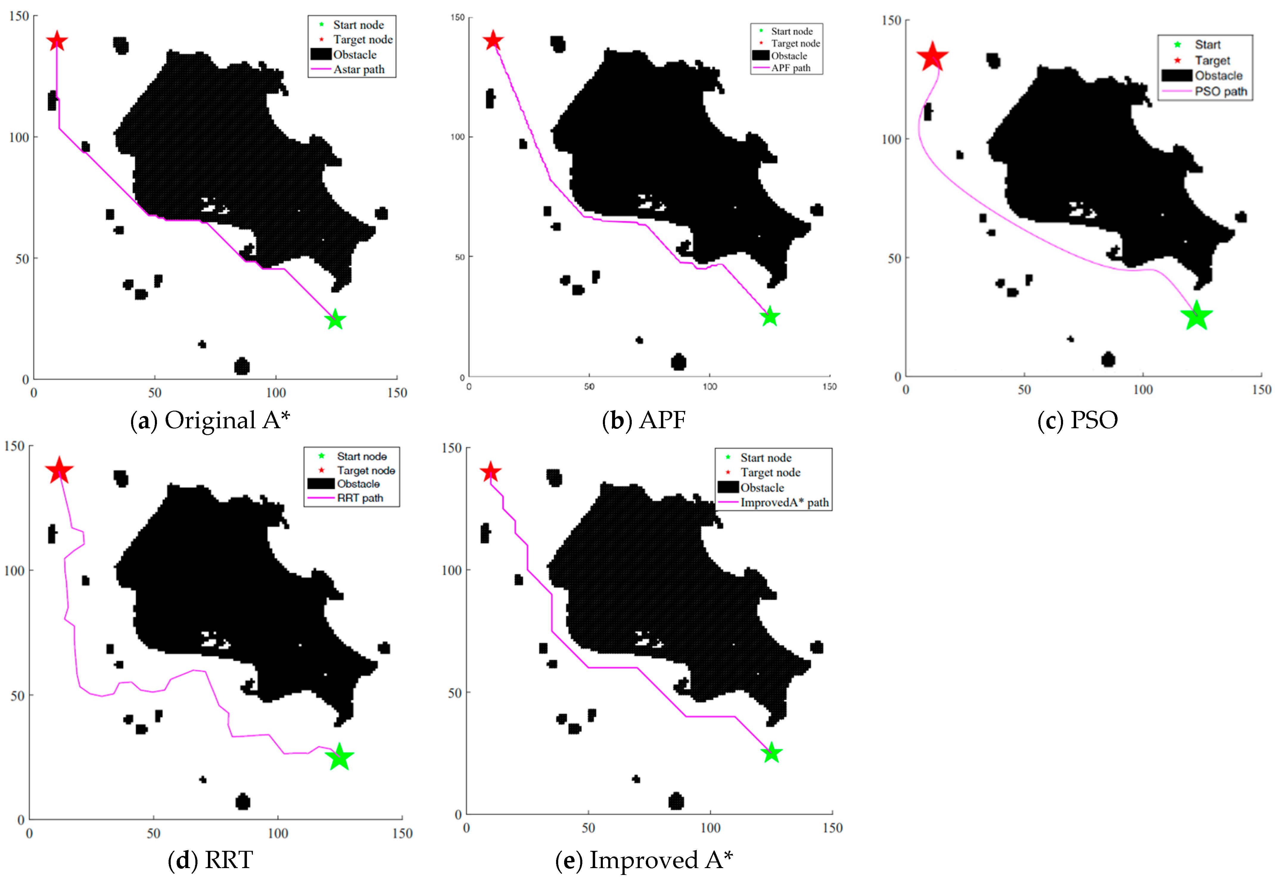
The proposed A* algorithm runs faster than other tested path-planning algorithms by ignoring perilous nodes and following the adaptive guidance angle. These improvements can reduce a lot of unnecessary computation while expanding the next nodes.

(2)

This study considered the impact of the current on the USV as forces exerted by obstacles on the USV by integrating the APF into the traditional A* algorithm. The proposed A* algorithm favorably deals with the ocean currents and obstacles and keeps an appropriate path–obstacle distance along the path.

(3)

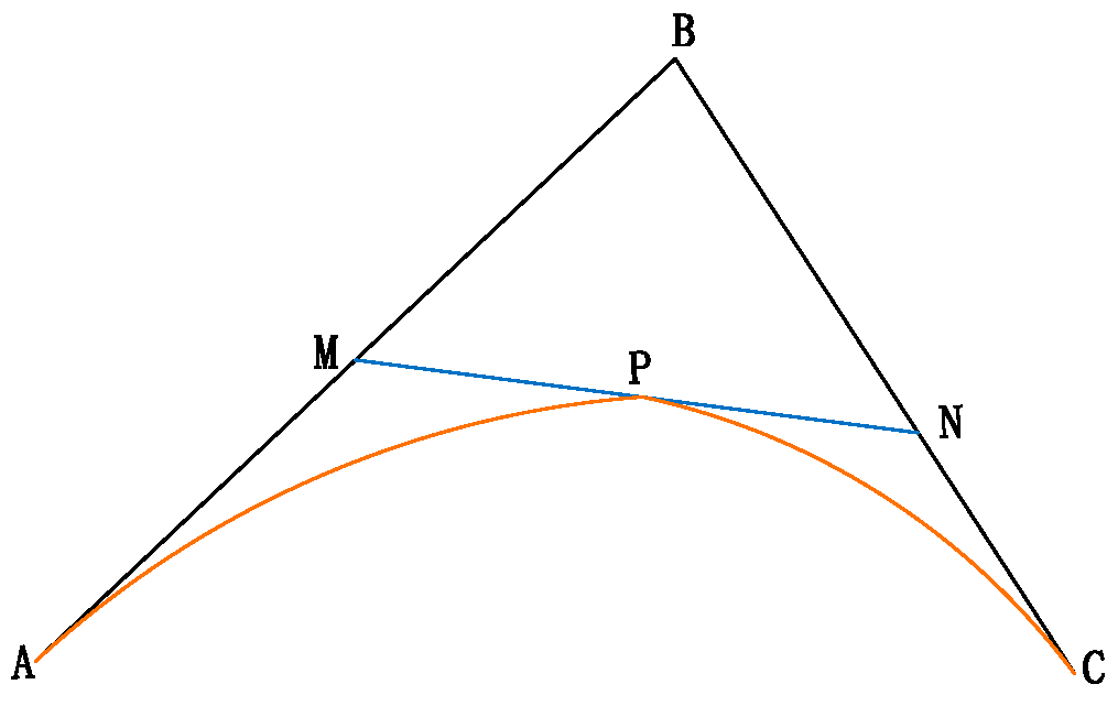
To smooth and optimize the path, this study adapted Bezier curves to address the problem of turning points. This optimization effectively reduces the number of turning points and the difficulty of controlling the steering of the USV when it is navigating in the currents.

This study provides a new perspective on producing an optimal path in complex marine environments. With the proposed A* algorithm, the information on ocean currents is introduced into the global path-planning stage to reduce the risk of collision with obstacles and grounding. However, although our study illustrates theoretical feasibility, its practical effectiveness in real-world applications has yet to be confirmed, as experimental field validation has not been performed.

Apart from the field experiments mentioned above, this study has several limitations that need to be addressed in future research. Firstly, this study focused solely on constant currents. The variations in the velocity and bearing of ocean currents and their effects on the behavior of the USV should be encompassed in subsequent investigations. Furthermore, more environmental factors, such as wind and waves, should be explored to bring this research closer to the real world.

References

1. Zhou, C.; Gu, S.; Wen, Y.; Du, Z.; Xiao, C.; Huang, L.; Zhu, M. The review unmanned surface vehicle path planning: Based on multi-modality constraint. Ocean Eng. 2020, 200, 107043. [Google Scholar] [CrossRef]
2. Chou, C.C.; Wang, C.N.; Hsu, H.P. A novel quantitative and qualitative model for forecasting the navigational risks of Maritime Autonomous Surface Ships. Ocean Eng. 2022, 248, 110852. [Google Scholar] [CrossRef]
3. Liu, J.; Wang, J. Overview of obstacle avoidance path planning algorithm for unmanned surface vehicle. Comput. Appl. Softw. 2020, 37, 11. [Google Scholar]
4. Zhang, W.; Shan, L.; Chang, L.; Dai, Y. SVF-RRT*: A Stream-Based VF-RRT* for USVs Path Planning Considering Ocean Currents. IEEE Robot. Autom. Lett. 2023, 8, 2413–2420. [Google Scholar] [CrossRef]
5. Hao, S.; Ma, W.; Han, Y.; Zheng, H.; Ma, D. Optimal path planning of unmanned surface vehicle under current environment. Ocean Eng. 2023, 286, 115591. [Google Scholar] [CrossRef]
6. Xing, B.; Yu, M.; Liu, Z.; Tan, Y.; Sun, Y.; Li, B. A Review of Path Planning for Unmanned Surface Vehicles. J. Mar. Sci. Technol. 2023, 11, 1556. [Google Scholar] [CrossRef]
7. Jin, K.; Zhu, H.; Gao, R.; Wang, J.; Wang, H.; Yi, H.; Shi, C.J.R. DEMRL: Dynamic estimation meta reinforcement learning for path following on unseen unmanned surface vehicle. Ocean Eng. 2023, 288, 115958. [Google Scholar] [CrossRef]
8. Peng, Z.; Li, J.; Han, B.; Gu, N. Safety-Certificated Line-of-Sight Guidance of Unmanned Surface Vehicles for Straight-Line Following in a Constrained Water Region Subject to Ocean Currents. J. Mar. Sci. Appl. 2023, 22, 602–613. [Google Scholar] [CrossRef]
9. Wang, Z.; Lu, R.; Wang, H. Finite-time trajectory tracking control of a class of nonlinear discrete-time systems. IEEE Trans. Syst. Man Cybern. 2017, 47, 1679–1687. [Google Scholar] [CrossRef]
10. Fnadi, M.; Du, W.; Plumet, F.; Benamar, F. Constrained Model Predictive Control for dynamic path tracking of a bi-steerable rover on slippery grounds. Control Eng. Pract. 2021, 107, 104693. [Google Scholar] [CrossRef]
11. Zhang, Y.; Liu, X.; Luo, M.; Yang, C. MPC-based 3-D trajectory tracking for an autonomous underwater vehicle with constraints in complex ocean environments. Ocean Eng. 2019, 189, 106309. [Google Scholar] [CrossRef]
12. Du, P.Z.; Yang, W.C.; Chen, Y.; Huang, S.H. Improved indirect adaptive line-of-sight guidance law for path following of under-actuated AUV subject to big ocean currents. Ocean Eng. 2023, 281, 114729. [Google Scholar] [CrossRef]
13. Yazdani, A.; MahmoudZadeh, S.; Yakimenko, O.; Wang, H. Perception-aware online trajectory generation for a prescribed manoeuvre of unmanned surface vehicle in cluttered unstructured environment. Robot. Auton. Syst. 2023, 169, 104508. [Google Scholar] [CrossRef]
14. Zhao, L.; Bai, Y. Data harvesting in uncharted waters: Interactive learning empowered path planning for USV-assisted maritime data collection under fully unknown environments. Ocean Eng. 2023, 287, 115781. [Google Scholar] [CrossRef]
15. Shu, Y.; Zhu, Y.; Xu, F.; Gan, L.; Lee, P.T.W.; Yin, J.; Chen, J. Path planning for ships assisted by the icebreaker in ice-covered waters in the Northern Sea Route based on optimal control. Ocean Eng. 2023, 267, 113182. [Google Scholar] [CrossRef]
16. Sun, B.; Zhang, W.; Li, S.; Zhu, X. Energy optimised D* AUV path planning with obstacle avoidance and ocean current environment. J. Navig. 2022, 75, 685–703. [Google Scholar] [CrossRef]
17. Liu, L.S.; Lin, J.F.; Yao, J.X.; He, D.W.; Zheng, J.S.; Huang, J.; Shi, P. Path planning for smart car based on Dijkstra algorithm and dynamic window approach. Wirel. Commun. Mob. Comput. 2021, 2021, 8881684. [Google Scholar] [CrossRef]
18. Zhang, H.; Tao, Y.; Zhu, W. Global Path Planning of Unmanned Surface Vehicle Based on Improved A-Star Algorithm. Sensors 2023, 23, 6647. [Google Scholar] [CrossRef]
19. Li, S.; Sun, B.; Zhu, X. Autonomous underwater vehicles dynamic path planning based on improved D∗ algorithm in ocean current environment. Chin. High Technol. Lett. 2022, 32, 84–92. [Google Scholar]
20. Gu, Q.; Zhen, R.; Liu, J.; Li, C. An improved RRT algorithm based on prior AIS information and DP compression for ship path planning. Ocean Eng. 2023, 279, 114595. [Google Scholar] [CrossRef]
21. Li, W.; Wang, L.; Zou, A.; Cai, J.; He, H.; Tan, T. Path Planning for UAV Based on Improved PRM. Energies 2022, 15, 7267. [Google Scholar] [CrossRef]
22. Feng, L.C.; Liang, H.W.; Du, M.B.; Yu, B. Guiding-area RRT path planning algorithm based on A* for intelligent vehicle. Comput. Syst. Appl. 2022, 26, 127–133. [Google Scholar]
23. Gan, Y.; Zhang, B.; Ke, C.; Zhu, X.; He, W.; Ihara, T. Research on robot motion planning based on RRT algorithm with nonholonomic constraints. Neural Process. Lett. 2021, 53, 3011–3029. [Google Scholar] [CrossRef]
24. Chi, W.; Ding, Z.; Wang, J.; Chen, G.; Sun, L. A generalized Voronoi diagram based efficient heuristic path planning method for RRTs in mobile robots. IEEE Trans. Ind. Electron. 2021, 99, 4926–4937. [Google Scholar] [CrossRef]
25. Xu, W.; Yang, Y.; Yu, L.; Zhu, L. A global path planning algorithm based on improved RRT. Control Decis. 2022, 37, 829–838. [Google Scholar]
26. Niu, Y.; Zhang, J.; Wang, Y.; Yang, H.; Mu, Y. A Review of Path Planning Algorithms for USV. In Proceedings of the 2021 International Conference on Autonomous Unmanned Systems, Changsha, China, 24–26 September 2021; Wu, M., Niu, Y., Gu, M., Cheng, J., Eds.; Springer: Singapore, 2021; pp. 263–273. [Google Scholar]
27. Niu, H.; Ji, Z.; Savvaris, A.; Tsourdos, A. Energy efficient path planning for unmanned surface vehicle inspatially-temporally variant environment. Ocean Eng. 2020, 196, 106766. [Google Scholar] [CrossRef]
28. Lars, L.; Kimb, J. Path planning of cooperating industrial robots using evolutionary Algorithms. Robot. Comput. Integer. Manuf. 2021, 67, 102053. [Google Scholar] [CrossRef]
29. Bai, X.; Li, B.; Xu, X.; Xiao, Y. USV path planning algorithm based on plant growth. Ocean Eng. 2023, 273, 113965. [Google Scholar] [CrossRef]
30. Wu, Y. Coordinated path planning for an unmanned aerial-aquatic vehicle (UAAV)and an autonomous underwater vehicle (AUV) in an underwater target strike mission. Ocean Eng. 2019, 182, 162–173. [Google Scholar] [CrossRef]
31. Ammar, A.; Bennaceur, H.; Chaari, I.; Koubaa, A.; Alajlan, M. Relaxed Dijkstra and A* with linear complexity for robot path planning problems in large scale grid environments. Soft Comput. 2016, 20, 4149–4171. [Google Scholar] [CrossRef]
32. Guo, B.; Kuang, Z.; Guan, J.; Hu, M.; Rao, L.; Sun, X. An improved a-star algorithm for complete coverage path planning of unmanned ships. Int. J. Pattern Recognit. Artif. Intell. 2022, 36, 2259009. [Google Scholar] [CrossRef]
33. Ma, Y.; Zhao, Y.; Li, Z.; Yan, X.; Bi, H.; Krolczyk, G. A new coverage path planning algorithm for unmanned surface mapping vehicle based on A-star based searching. Appl. Ocean Res. 2022, 123, 103163. [Google Scholar] [CrossRef]
34. Wang, C.; Wang, L.; Qin, J.; Wu, Z.; Duan, L.; Li, Z.; Wang, Q. Path planning of automated guided vehicles based on improved A-Star algorithm. In Proceedings of the 2015 IEEE International Conference on Information and Automation, Lijiang, China, 8–10 August 2015; pp. 2071–2076. [Google Scholar]
35. Daniel, K.; Nash, A.; Koenig, S.; Felner, A. Theta*: Any-angle path planning on grids. J. Artif. Intell. Res. 2010, 39, 533–579. [Google Scholar] [CrossRef]
36. Gan, L.; Yan, Z.; Zhang, L.; Liu, K.; Zheng, Y.; Zhou, C.; Shu, Y. Ship path planning based on safety potential field in inland rivers. Ocean Eng. 2022, 260, 111928. [Google Scholar] [CrossRef]
37. Sang, H.; You, Y.; Sun, X.; Zhou, Y.; Liu, F. The hybrid path planning algorithm based on improved A* and artificial potential field for unmanned surface vehicle formations. Ocean Eng. 2021, 223, 108709. [Google Scholar] [CrossRef]
38. Xie, L.; Xue, S.; Zhang, J.; Zhang, M.; Tian, W.; Haugen, S. A path planning approach based on multi-direction A* algorithm for ships navigating within wind farm waters. Ocean Eng. 2019, 184, 311–322. [Google Scholar] [CrossRef]
39. Liu, Y.; Bucknall, R. Path planning algorithm for unmanned surface vehicle formations in a practical maritime environment. Ocean Eng. 2015, 97, 126–144. [Google Scholar] [CrossRef]
40. Zhou, L.F.; Kong, M.Y. 3D obstacle-avoidance for an unmanned aerial vehicle based on the improved artificial potential field method. J. East China Norm. Univ. (Nat. Sci.) 2022, 2022, 54–67. [Google Scholar]
41. Pan, Z.; Zhang, C.; Xia, Y.; Xiong, H.; Shao, X. An improved artificial potential field method for path planning and formation control of the multi-UAV systems. IEEE Trans. Circuits Syst. II Express Briefs 2021, 69, 1129–1133. [Google Scholar] [CrossRef]
42. Wang, N.; Xu, H.; Li, C.; Yin, J.C. Hierarchical path planning of unmanned surface vehicles: A fuzzy artificial potential field approach. Int. J. Fuzzy Syst. 2020, 23, 1797–1808. [Google Scholar] [CrossRef]
43. Zeng, Z.; Sammut, K.; Lian, L.; He, F.; Lammas, A.; Tang, Y. A comparison of optimization techniques for AUV path planning in environments with ocean currents. Robot. Auton. Syst. 2016, 82, 61–72. [Google Scholar] [CrossRef]
44. Yoo, B.; Kim, J. Path optimization for marine vehicles in ocean currents using reinforcement learning. J. Mar. Sci. Technol. 2016, 21, 334–343. [Google Scholar] [CrossRef]
45. Lee, T.; Kim, H.; Chung, H.; Bang, Y.; Myung, H. Energy efficient path planning for a marine surface vehicle considering heading angle. Ocean Eng. 2015, 107, 118–131. [Google Scholar] [CrossRef]
46. Subramani, D.N.; Lermusiaux, P.F. Energy-optimal path planning by stochastic dynamically orthogonal level-set optimization. Ocean Model. 2016, 100, 57–77. [Google Scholar] [CrossRef]
47. Gao, B.; Xu, D.; Zhang, F.; Yan, W. Method of Designing Optimal Smooth Way for Vehicle. J. Syst. Simul. 2010, 22, 957–961. [Google Scholar]
48. Liu, Y.; Gu, Y.; Li, X. Optimal design of path algorithm for unmanned surface vessel under complex sea conditions. J. Mil. Transp. Univ. 2021, 23, 83–87. [Google Scholar]
49. Ma, Y.; Hu, M.; Yan, X. Multi-objective path planning for unmanned surface vehicle with currents effects. ISA Trans. 2018, 75, 137–156. [Google Scholar] [CrossRef]
50. Ma, Y.; Mao, Z.; Wang, T.; Qin, J.; Ding, W.; Meng, X. Obstacle avoidance path planning of unmanned submarine vehicle in ocean current environment based on improved firework-ant colony algorithm. Comput. Electr. Eng. 2020, 87, 106773. [Google Scholar] [CrossRef]
51. Xu, P.; Ding, X.; Cao, Q. Research on global path planning of unmanned surface vehicle based on environmental optimization. Shipbuild. China 2022, 63, 206–220. [Google Scholar]
52. Yu, J.; Chen, Z.; Zhao, Z.; Yao, P.; Xu, J. A traversal multi-target path planning method for multi-unmanned surface vessels in space-varying ocean current. Ocean Eng. 2023, 278, 114423. [Google Scholar] [CrossRef]
53. MahmoudZadeh, S.; Abbasi, A.; Yazdani, A.; Wang, H.; Liu, Y. Uninterrupted path planning system for Multi-USV sampling mission in a cluttered ocean environment. Ocean Eng. 2022, 254, 111328. [Google Scholar] [CrossRef]
54. Zhao, L.; Bai, Y.; Paik, J.K. Achieving optimal-dynamic path planning for unmanned surface vehicles: A rational multi-objective approach and a sensory-vector re-planner. Ocean Eng. 2023, 286, 115433. [Google Scholar] [CrossRef]
55. Liu, C.; Mao, Q.; Chu, X.; Xie, S. An improved A-star algorithm considering water current, traffic separation and berthing for vessel path planning. Appl. Sci. 2019, 9, 1057. [Google Scholar] [CrossRef]
56. Xie, X.; Liu, C.; Wei, Z. Ship path planning in complex water areas under the influence of marine meteorological environment. J. Chongqing Jiaotong Univ. (Nat. Sci.) 2021, 40, 1–7, 20. [Google Scholar]
57. Singh, Y.; Sharma, S.; Sutton, R.; Hatton, D.; Khan, A. A constrained A* approach towards optimal path planning for an unmanned surface vehicle in a maritime environment containing dynamic obstacles and ocean currents. Ocean Eng. 2018, 169, 187–201. [Google Scholar] [CrossRef]
58. Xie, X.; Wang, Y.; He, A.; Pan, W.; Xu, X. Ship path planning and algorithm considering the effect of wind, wave and current. J. Chongqing Jiaotong Univ. (Nat. Sci.) 2022, 41, 1–8. [Google Scholar]
59. Wang, F.; Bai, Y.; Zhao, L. Physical Consistent Path Planning for Unmanned Surface Vehicles under Complex Marine Environment. J. Mar. Sci. Eng. 2023, 11, 1164. [Google Scholar] [CrossRef]
60. Wang, Y.; Liang, X.; Li, B.; Yu, X. Research and implementation of global path planning for unmanned surface vehicle based on electronic chart. In Recent Developments in Mechatronics and Intelligent Robotics, Proceedings of the International Conference on Mechatronics and Intelligent Robotics (ICMIR2017), Kunming, China, 20–21 May 2017; Springer: Berlin/Heidelberg, Germany, 2017; Volume 1, pp. 534–539. [Google Scholar]
61. Xing, B.; Wang, X.; Yang, L.; Liu, Z.; Wu, Q. An Algorithm of Complete Coverage Path Planning for Unmanned Surface Vehicle Based on Reinforcement Learning. J. Mar. Sci. Eng. 2023, 11, 645. [Google Scholar] [CrossRef]
62. Alvarez, A.; Caiti, A.; Onken, R. Evolutionary path planning for autonomous underwater vehicles in a variable ocean. IEEE J. Ocean. Eng. 2004, 29, 418–429. [Google Scholar] [CrossRef]
63. Hu, D.; Chen, X.; Zhang, S.; Li, Y. Characteristics of tide and residual current south of Dongsha island in South China Sea. J. Army Eng. Univ. PLA (Chin.) 2015, 16, 368–373. [Google Scholar]
64. Hu, S.; Xiao, S.; Yang, J.; Zhang, Z.; Zhang, K.; Zhu, Y.; Zhang, Y. AUV Path Planning Considering Ocean Current Disturbance Based on Cloud Desktop Technology. Sensors 2023, 23, 7510. [Google Scholar] [CrossRef] [PubMed]
65. Song, B.; Wang, Z.; Zou, L. An improved PSO algorithm for smooth path planning of mobile robots using continuous high-degree Bezier curve. Appl. Soft Comput. 2021, 100, 106960. [Google Scholar] [CrossRef]
Figure 1. The environmental map: (a) original map; (b) grid map.
Jmse 12 00285 g001
Figure 3. USV’s movements in currents.
Jmse 12 00285 g003
Figure 4. Node-searching approach of the A* algorithm.
Jmse 12 00285 g004
Figure 5. Different distance calculation methods.
Jmse 12 00285 g005
Figure 6. Path around the apex of obstacles (black grids): (a,b) crossing the vertices of obstacles from start (green grids) to goal (red grids); (c,d) bypassing the vertices of obstacles.
Jmse 12 00285 g006
Figure 7. Diagram of perilous nodes.
Jmse 12 00285 g007
Figure 8. Adaptive guidance angle and opposite node number.
Jmse 12 00285 g008
Figure 9. The path of the USV under the influence of a left-side current.
Jmse 12 00285 g009
Figure 10. Selection of path nodes for different currents.
Jmse 12 00285 g010
Figure 11. Second-order Bezier curve smoothing.
Jmse 12 00285 g011
Figure 12. Flowchart of the improved A* algorithm.
Jmse 12 00285 g012
Figure 13. Paths with different algorithms in simulation 1.
Jmse 12 00285 g013
Figure 14. Paths with different algorithms in simulation 2.
Jmse 12 00285 g014