Extracted Spectral Signatures from the Water Column as a Tool for the Prediction of the Structure of a Marine Microbial Community

Abstract

In this communication, we present an innovative approach leveraging advanced Machine Learning (ML) and Artificial Intelligence (AI) techniques, specifically the Non-Negative Matrix Factorization (NMF) method, to analyze downward and upward light spectra collected by Hyperspectral Ocean Color Radiometer (HyperOCR, HOCR) sensors in the water column. Our work focuses on the development of a robust and efficient tool for unraveling the structure and activities of natural microbial assemblages in the ocean. By applying the NMF method to HyperOCR data, we successfully extracted five spectral signatures, representing unique patterns in the data. These signatures were instrumental in predicting the abundances of various microbial components, including bacteria, heterotrophic nanoflagellates, and picoeukaryotes, showcasing the potential of ML and AI in advancing oceanographic studies. To validate these methods, the study area included a shallow coastal area under the influence of freshwater inflow and an open offshore area with a depth of 100 m. The study sites in coastal and offshore waters (Kaštela Bay and Stončica Vis, respectively) had significantly different hydrographic and microbiological characteristics. Kaštela Bay had lower temperatures and salinity than the site on Vis. We have demonstrated prediction of the structure of the microbial community through application of different AI and ML methods with specific HOCR sensors.

1. Introduction

Understanding the dynamics of primary producers in terms of their composition and community structure in space and time is very important as it indicates their health and their responses to changes in climate. Aquatic remote sensing as a tool faces challenges as these environments are highly diverse, so difficulties occur where absorption/reflection is affected by higher concentrations of inorganic particles and/or colored (fluorescent) dissolved organic matter [1,2,3,4]. In recent years, in situ measurements of the hyperspectral optical properties of aquatic microbial consortia have gained momentum as changes in the community type, size classes, distribution or pigments can be obtained from analyzing changes in their optical properties from various multispectral remote sensing sources [5,6,7,8]. It has been found that the spectral characteristics of phytoplankton light absorption coefficients are directly related to pigment composition, concentration, and cell structure [9,10,11]. Important contributions to understanding vertical distribution and dynamics of phytoplankton, pigments, and colored dissolved organic matter (CDOM) were obtained from studies of data collected by Biogeochemical-Argo floats [12]. The implications of global warming arising from such large-scale operations on ocean ecosystems necessitate more detailed insights, and traditional approaches fall short in providing the required temporal and spatial resolutions. We decided to use a different approach. Here, we employ ML protocols, specifically NMF, to analyze spectral changes in the water column, as measured by HyperOCR sensors. NMF is a dimensionality reduction and feature extraction method that factorizes the input matrix into two matrices, which, when multiplied again, results in the original matrix [13]. In our project, we factorize spectral curves from HyperOCR sensors with the intention of discovering latent patterns in the sensor data [14]. A similar approach is used when dealing with mutational data, where a simple count matrix is factorized into two matrices, discovering underlying biological mechanisms at play [15].

HyperOCR sensors capture the adsorption (downwelling radiation) and reflection (upwelling radiation) of light, offering a comprehensive view of the water column. Our objective is to explore the wealth of information that can be gleaned by correlating spectral changes with various environmental parameters, thus highlighting the pivotal role of ML and AI in enhancing our understanding of ocean dynamics. The consequences of present global warming trends include pronounced ocean stratification, geographical shifts, and a decrease in nutrient supply with phytoplankton community shifts towards small phytoplankton. Increased concentrations of atmospheric CO₂ enhance ocean acidification [16]. Small phytoplankton might find preferable conditions in the interstices of such organic patches balancing the gap in the reduced production because of warming and acidification.

We applied NMF protocols [17] in analyzing spectral changes in light in the water column as a new tool in oceanography. For understanding primary production in the oceans, it is essential to collect much more detailed information with emerging technologies on both temporal and spatial scales, which is impossible with traditional approaches. This is the reason that we wanted to explore the amount of information we can obtain from analyzing spectral changes in the water column and correlating them to other measured parameters, as vertical profiles of HyperOCR downward and upward sensors measure the adsorption of light and reflection of light throughout the water column, respectively, thus providing a very detailed picture of changes in the water column.

The synergy of AI and oceanography illustrates the potential for technological advancements to address environmental challenges. ML algorithms serve as a bridge connecting intricate sensor data with meaningful insights and paving the way for a new era in oceanographic research.

2. Materials and Methods

In the realm of scientific methodologies, the infusion of ML methodologies stands as a testament to the symbiotic relationship between AI and domain-specific research. The development of models such as NMF amplifies the precision of data analysis, showcasing the capacity of AI to contribute significantly to advancing scientific discovery. Our study, conducted in the central Adriatic Sea, integrates ML techniques into the analysis of data collected through advanced sensor systems. The NMF model, developed using a training dataset of 5397 HOCR curves, successfully extracts five spectral signatures, each revealing distinct patterns across the visible spectrum. These signatures demonstrate unique associations with depth, sensor type (downwelling or upwelling), and environmental parameters, underscoring the versatility of ML in discerning complex patterns in oceanographic data.

2.1. Sampling and Incubations

This study was conducted on 12 and 13 June 2023 in the central Adriatic Sea in the vicinity of Split and Vis, Croatia, at a site in Kaštela Bay (12 June, 43°31′33.9″ N, 16°23′17.6″ E, depth 38.4 m) and near Stončica lighthouse on Vis Island (13 June, 43°03′32.8″ N, 16°17′19.7″ E, depth 102.9 m). Sampling depths in Kaštela Bay were 0, 5, 10, 15, 20, 25, and 28 m (K0, K5, K10, K15, K20, K25, K28) and at Stončica-Vis station, the water column was sampled at 0, 5, 10, 20, 30, 50, and 100 m (V0, V5, V10, V20, V30, V50, V100). All samples were taken at predetermined depths using a 5 L Niskin water sampler (General Oceanics, Miami, FL, USA). Before subsampling, all bottles were rinsed three times with seawater from the sampler.

2.2. Fluorometric Determination of Chlorophyll and Radiometric Determination of Chlorophyll Absorbance Spectra

Five hundred (500) mL samples were filtered on 45 mm GF/F glass fiber filters, folded in half, and stored at −20 °C until chlorophyll extraction in the onshore lab. Upon arrival at the laboratory (within 48 h), the filters were ground in a few mL of 90% acetone in a glass homogenizer with a motor-driven Teflon pestle for 1 min in an ice bath and under subdued light. After grinding, the extract was carefully transferred to a stoppered and graduated centrifuge tube. The glass homogenizer and the pestle were rinsed with 90% acetone and the rinsed volumes were added to the centrifuge tube. The extract volume in the centrifuge tube comprised exactly 10 mL of 90% acetone. Immediately before measurement, the extracts were thoroughly mixed and centrifuged for 10 min at 500× g. The fluorometer was calibrated by using a commercial solution of pure Chlorophyll a (Sigma-Aldrich C5733 Chlorophyll a, Merck d.o.o., Zagreb, Croatia). Sample extracts were transferred from the centrifuge tubes to the fluorometer cuvette by careful decanting. The fluorescence of the sample extract was measured against a 90% acetone blank. After measurements, 0.2 mL 1% v/v hydrochloric acid was added to the cuvette and mixed. After 2–5 min., the fluorescence of the sample extract was measured again against a 90% acetone blank. The concentration of Chlorophyll a and phaeopigments was calculated according to the equations of Holm-Hansen et al. [18].

After fluorescence measurements, a 3 mL aliquot of the chlorophyll extract was transferred to an optical-grade 10 mm analysis cell to measure light absorbance spectra using an Apogee SP-200 spectroradiometer (Apogee Instruments, Inc., North Logan, UT, USA).

2.3. Flow Cytometry

For the flow cytometry count of autotrophic cells, 2 mL of preserved samples in 0.5% glutaraldehyde were frozen at -80 °C and stored until analysis on a Cytoflex cytometer (with a 488 nm laser and a flow rate of 60 µL/min for 200 s) (Beckman Coulter D.O.O., Zagreb, Croatia). Autotrophic cells were divided into groups (Synechococcus, Prochlorococcus, and picoeukaryotes) that were distinguished according to light scattering, red emission of cellular chlorophyll content, and orange emission of phycoerythrin-rich cells. Abundances of Sybr Green-I-stained bacteria, high-nucleic-acid-content (HNA) bacteria, low-nucleic-acid-content (LNA) bacteria, and heterotrophic nanoflagellates (HNF) were also determined using flow cytometry [19], and the samples were preserved in 2% formaldehyde and stored at 4 °C until analysis.

2.4. Light Microscopy

Identification and abundance of phytoplankton communities have been determined using the Utermöhl sedimentation method [20]. Water samples of 250 mL were collected using Nansen bottles and then preserved by adding formaldehyde to achieve a final concentration of 2% formaldehyde–seawater solution. After this preservation, subsamples of 25 mL each were stored in counting chambers for 24 h. For subsequent analysis, two transects within the sedimentation chamber were selected for counting, which was facilitated by an inverted microscope. The choice of magnification, either ×200 or ×400, was based on the size of the species being observed.

2.5. Solar Radiation, Salinity, Temperature, and Depth Measurements

In this study, we used two vertical profilers and a reference hyperspectral curve station. The first vertical profiler (Seabird SBE 25plus Sealogger CTD, EIVA, Skanderborg, Denmark) measured conductivity, temperature, and depth profiles. The second vertical profiler measured downward and upward irradiance profiles with two Hyperspectral Ocean Color Radiometer (Seabird HOCR) (EIVA, Skanderborg, Denmark) sensors calibrated for measurements of downwelling and upwelling radiation with optical data in the range of 350–1200 nm (extended range). HOCR sensors were mounted on a frame equipped with an Seabird SBE 39plus temperature (EIVA, Skanderborg, Denmark) (using an external thermistor), depth (using a 100 m strain gauge pressure sensor), and time sensors. Measured data were recorded in a custom-built data logger built by MARINIX Ocean Tech AS (Kristiansand, Norway). The third part of this system was a hyperspectral color radiometer sensor (Apogee PS-200 (Apogee Instruments, Inc., North Logan, UT, USA) laboratory hyperspectral radiometer, 300–850 nm range, 0.5 nm sensitivity) that was installed on the highest point on the vessel with the sensor pointed upwards vertically to measure reference surface light spectra during the vertical profile casts of the water column with HOCR.

2.6. Preprocessing of Hyperspectral Curves Using Reference Measurements

On both stations (Kaštela and Vis), we utilized multiple sensor systems for data collection. The purpose of Apogee HOCR, positioned on the highest point on the vessel, was to collect HOCR curves representing reference data (at a particular time point) that can be paired with vertical profiler data. The reference curve was then used to normalize the data from the vertical profiler, resulting in curves whose values range from 0 to 100, representing the percentage of the reference curve at a certain nanometer.

2.7. Computational Rquirements

All model training, the genetic algorithm, and NMF were run in Python 3.10.11 on regular laptop with the following specifications: Lenovo IdeaPad 3—17ITL6 laptop type 82H9, 17-inch, 11th Generation Intel Core i5—1135G7, Intel iRIS graphics, memory 2 × 8 GB DDR4-3200, hard drive 512 GB SSD PCIe.

3. Results

Our findings showcase the ML-based model’s efficacy in predicting microbial community structures. By applying the extracted spectral signatures, we achieved a minimal root mean square error (RMSE) in predicting bacteria, heterotrophic nanoflagellates, and picoeukaryotes. Notably, ML predictions exhibited intermediate RMSE values for Prochlorococcus and a larger RMSE for Synechococcus and HNA bacteria, shedding light on the varying predictability across different microbial components.

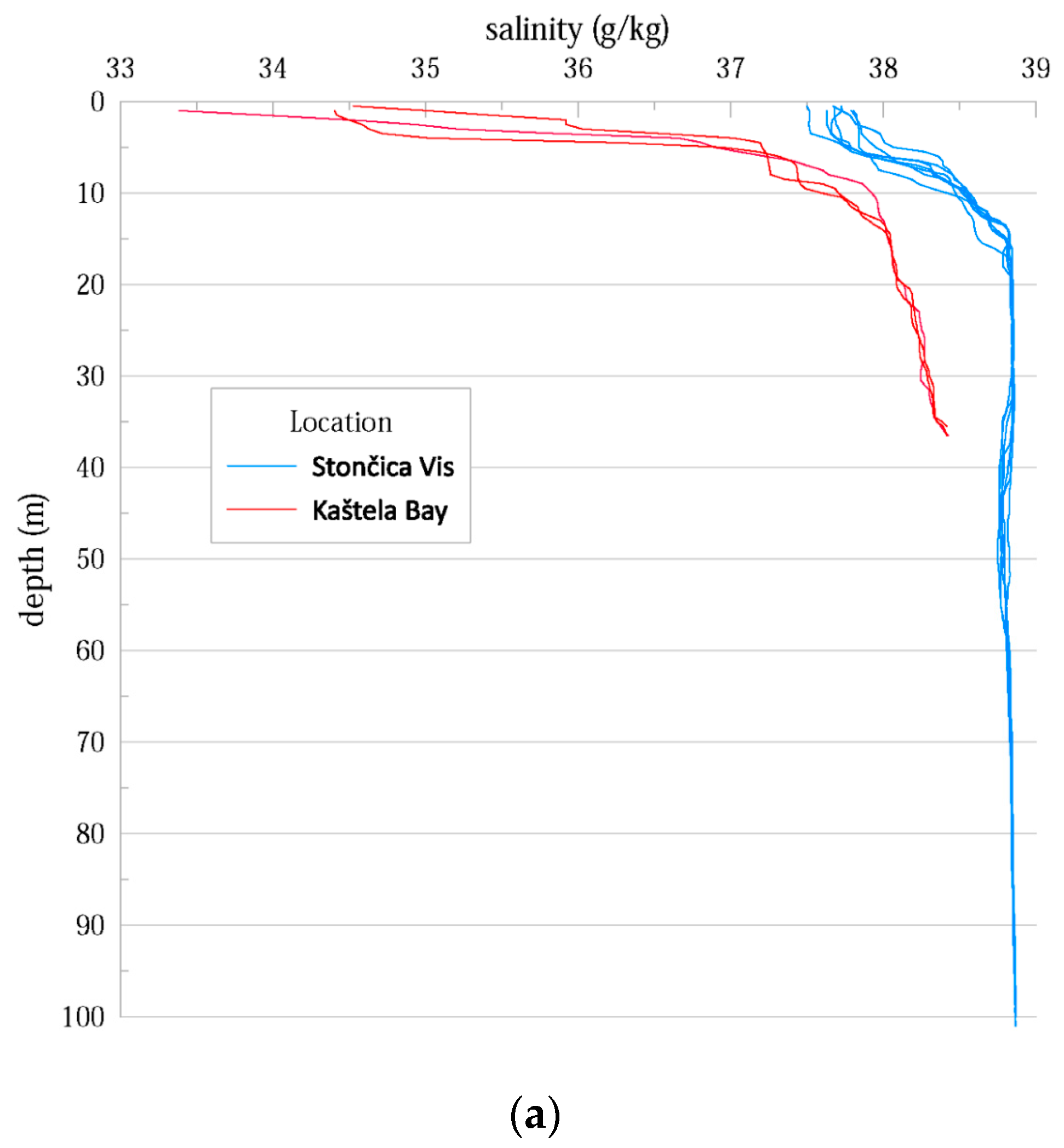
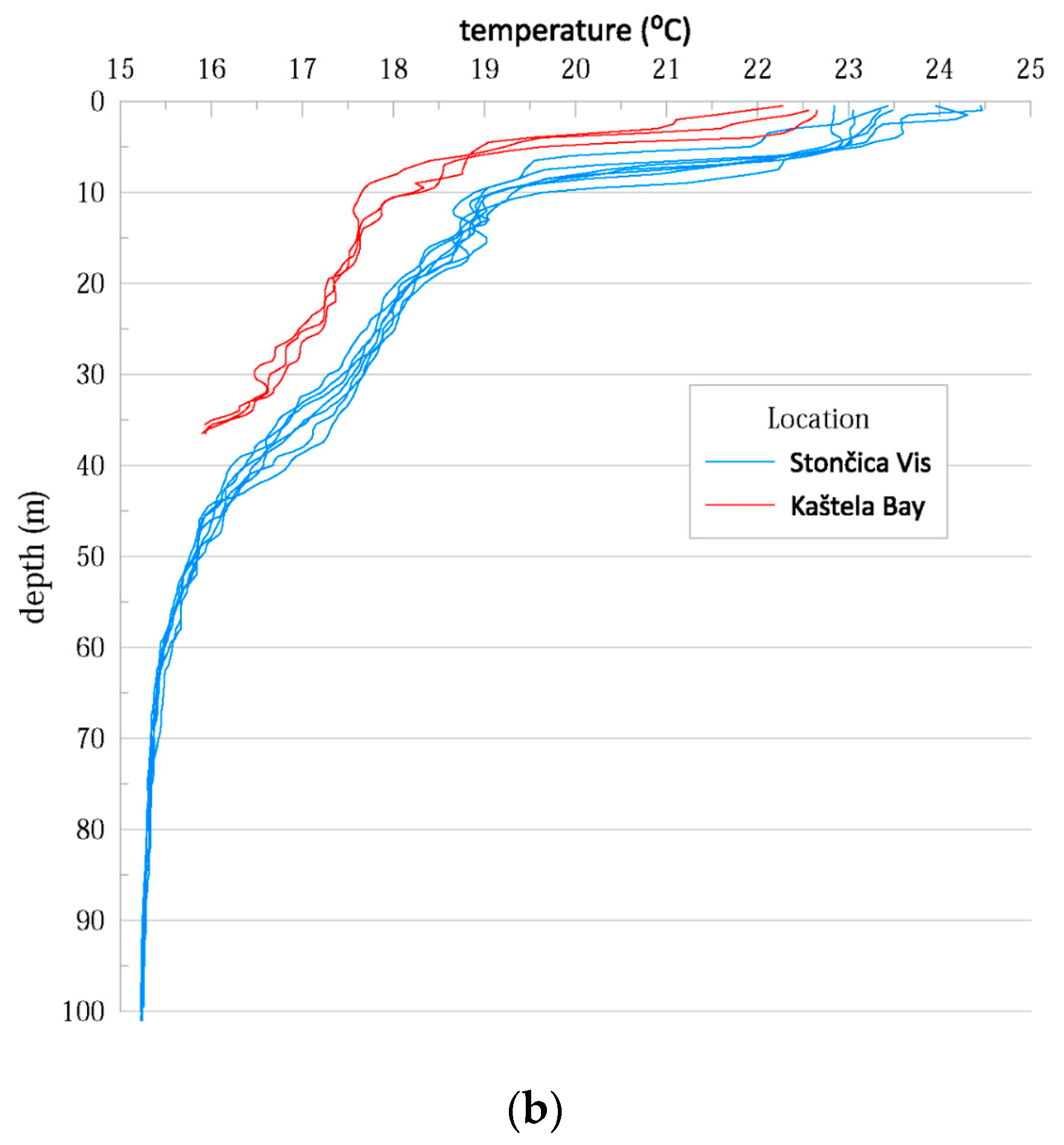
3.1. Hydrographic Properties of the Water Column

To characterize the study sites, we examined the differences in thermohaline properties at the study sites in Kaštela Bay and Stončica-Vis. The onset of seasonal stratification was observed in both vertical temperature profiles, with a warmer layer at the top and a colder one at the bottom. This is due to surface warming and relatively weak wind forcing during the warm period of the year (July to September) [21]. Both salinity and temperature were lower in Kaštela Bay than in Stončica-Vis (oligotrophic site in the open sea), indicating the different characteristics of the two studied sites (Figure A1). Since Kaštela Bay of Kaštela is surrounded by urban development and intense human activity (near the port of Split), with a significant freshwater discharge of the river Jadro (average annual inflow of ~l0 m³ s⁻¹) and several submarine sources of lower intensity, it can be assumed that these have an influence on the hydrographic characteristics of the seawater body [21].

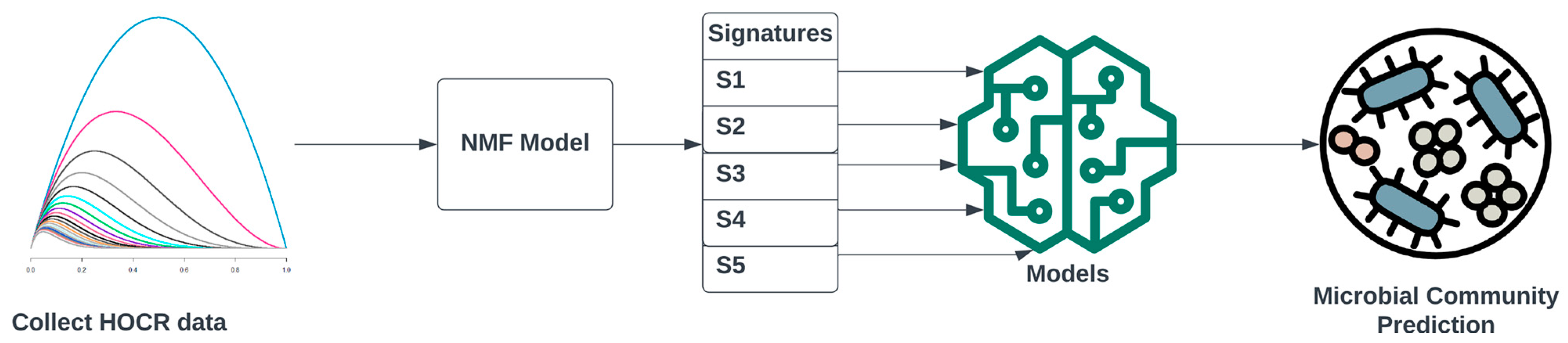
3.2. Developing HOCR Signatures Using a Non-Negative Factorization Model on Training Data

Using our custom-built vertical profiler and prior to the experiment, we collected HOCR curves at different locations in the southern Adriatic Sea in the vicinity of the Island of Mljet, and at different time points of the day. This resulted in a dataset containing 5397 HOCR curves which we used as a training dataset for model development. The model we developed is based on the Non-Negative Matrix Factorization method (NMF) [14,22], which uses the input data (HOCR) curves in order to factorize them into two matrices. The first matrix (H) represents “spectral signatures”, which are unique patterns in the data discovered by the method. The second matrix (W) represents the weights of each curve (sample) towards each signature. To determine the optimal number of signatures in the data, we applied NMF multiple times with different numbers of signatures (2 to 10), measuring reconstruction error. The reconstruction error was measured using two methods (Frobenius Norm and Kullback–Leibler) [23] and resulted in an optimal number of signatures K = 5 (Figure 1a).

Once the optimal number of signatures was found, we fitted the model using the training data and the following hyperparameters: n_components = 5, init = ‘nndsvda’, solver = ‘cd’, beta_loss = ‘frobenius’, max_iter = 10,000. The model successfully extracted five spectral signatures (S1–S5), representing distinct patterns in the data. S1 showed the highest peak at 359 nm, followed by the peak at 597 nm (Figure 1b, blue curve). S2 showed a single peak at 506 nm (Figure 1b, orange curve). S3 was characterized by a similar curve as S2; however, there was a smaller peak at 490 nm (Figure 1b, green curve). S4 captured a wide spectrum range from 350 nm to 580 nm in an almost uniform fashion (Figure 1b, red curve). S5 was characterized by a spectral curve spanning from 350 nm to 560 nm, having two peaks at 393 nm and 496 nm (Figure 1b, purple curve). Since the training data contained the HOCR curves coming from downward (DW—downwelling radiation) and upward (UW—upwelling radiation) sensors, we compared the extracted signatures between those two sensors. Downward (DW) sensor data are mostly characterized by S3, followed by S5, whereas upwelling sensor data showed a more complex distribution of signature enrichment (Figure 1c). Next, we computed kernel density estimation (KDE) for a probability density between signature enrichment and depth. We visualized the KDE for each signature–depth pair and observed that S1 extracted from the UW sensor showed a negative linear correlation towards depth. The S1 signature from the DW sensor showed enriched density around depths of 0 and 100 m. Spectral signature S2 extracted from the UW sensor showed almost no patterns with respect to depth; however, most of the enrichment was located around 20 m depth. S3 extracted from the DW sensor showed a linear pattern with respect to depth, with increased density between 0 and 40 m depth, whereas S3 extracted from UW showed increased density around 90 m depth. S4 extracted from UW curves showed limited density, whereas signature S4 extracted from DW curves showed increased density across the entire measured water column (0–100 m), particularly around 10 m depth. S5 extracted from UW curves showed a negative linear pattern with respect to depth and increased density around 90 m depth. S5 extracted from the DW HOCR curve showed increased density throughout the entire measured water column (0–100 m), with an increase in density of around 20 m of depth (Figure 1d). Finally, the five extracted spectral signatures showed unique patterns, capturing complex patterns across the entire visible spectrum, indicating differences between UW and DW sensors and showing an association with depth. A summary of signature characteristics can be found in

Table 1. Summary of signature characteristics: UW, upwelling sensor; DW, downwelling sensor; PE, picoeukaryotes; PCO, Prochlorococcus; BAC, bacteria; HNAN, heterotrophic nanoflagellates; SNCO Synechococcus.

Signature	Spectrum Assoc.	Depth Assoc. (Training Data)	Microbial Assoc. Kaštela	Microbial Assoc. Stončica Vis
S1	Two peaks at 359 nm and 597 nm	UW: Positive	UW: PE (positive), PCO (positive), BAC (negative)	UW: SNCO (negative), HNAN (positive), BAC (negative), PCO (positive)
		DW: Minimal enrichment, around 40 m	DW: SNCO (positive), HNAN (positive), PE (positive), BAC (negative), PCO (negative)	DW: SNCO (negative),HNAN (positive), PE (positive), BAC (negative)
S2	High-intensity broad peak at 506 nm	UW: Minimal enrichment	UW: HNAN (positive), BAC (positive)	UW: HNAN (positive) PE (positive)
		DW: Negative convex	DW: PCO (negative), PE (negative), HNAN (negative),	DW: PE(positive), PCO (negative)
S3	Small peak at 490 nm	UW: Enriched at all depths (0–100 m), mostly around 90 m	UW: HNAN (negative), PE (negative), SNCO (negative)	UW: SNCO (positive), BAC (positive), HNAN (positive), PCO (negative)
		DW: Positive, mainly between 0–40 m	DW: SNCO (negative), PCO (positive)	DW: PCO (positive), PE (negative)
S4	Low-intensity, almost uniform at 350–580 nm	UW: Positive, mostly around 80 m	UW: BAC (positive)	UW: SNCO (negative), HNAN (negative),BAC (negative), PCO (positive)
		DW: Highly enriched in 0–20 m, minimal in depth > 20 m	DW: SNCO (negative), HNAN (negative), PE (negative)	DW: HNAN (negative), PCO (negative)
S5	Low-intensity, Covering a broad spectrum of 350–560 nm	UW: Negative, mostly around 80 m	UW: SNCO (positive), HNAN (positive), BAC (positive),	UW: HNAN (negative), PCO (negative)
		DW: Enriched at all depths (0–100 m)	DW: HNAN (negative), PE (negative), PCO (negative)	DW: PE (negative), PCO (negative), BAC (positive), SNCO (positive)

.

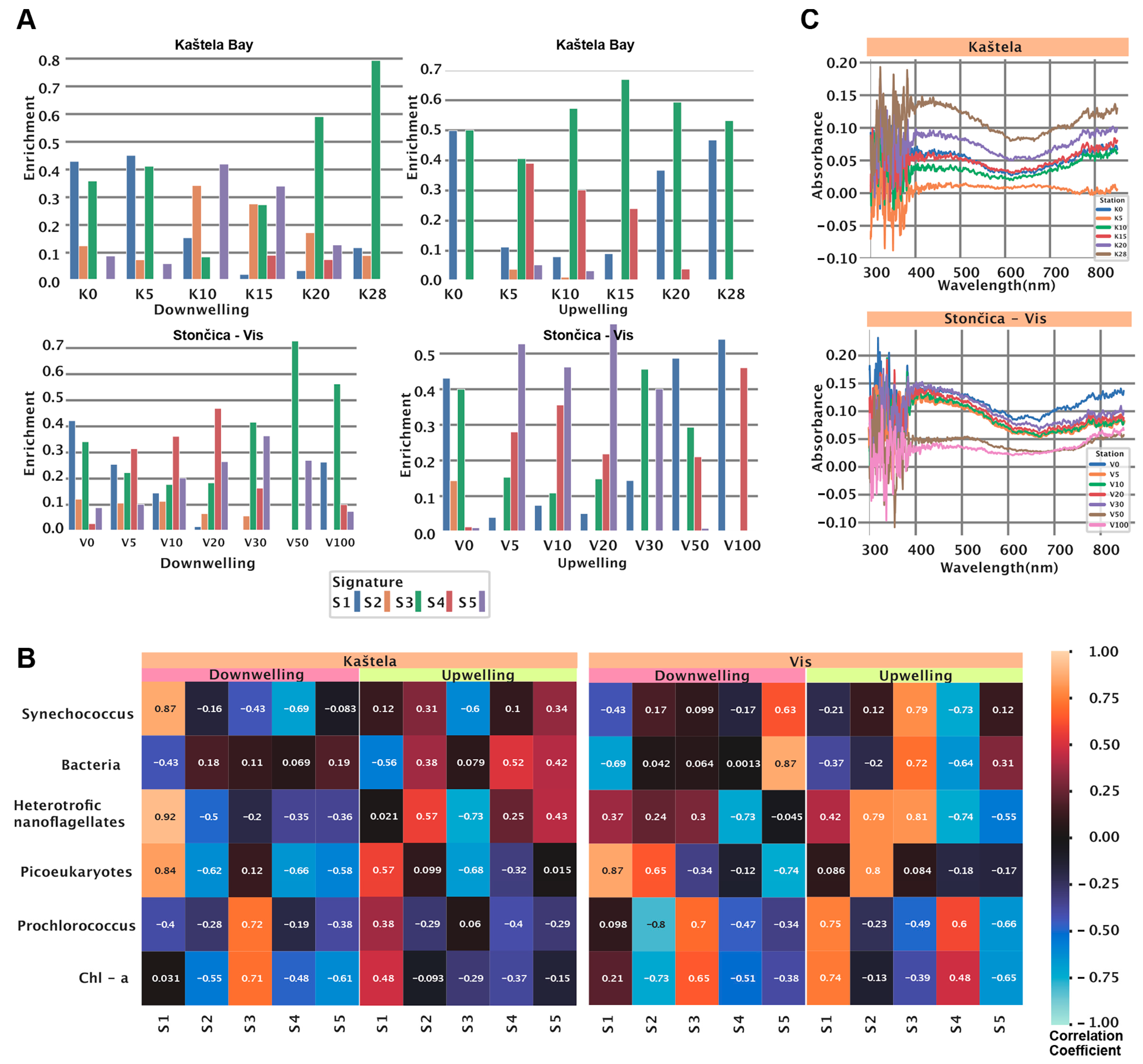
3.3. HOCR Spectral Signatures at the Study Locations

We measured seven HOCR profiles at two investigated stations, Kaštela Bay and Stončica-Vis. From HOCR profiles, we extracted five spectral signatures (Figure 1). We used one measurement for samples at each depth for each site. Signature S1 had strong peaks at 359 nm and 597 nm; the upwelling (UW) signature had a positive correlation with depth, while the downwelling (DW) signature S1 was present at 0 m and a little at 100 m. Signature S2 had a strong peak at 506 nm with no presence in UW profiles, while the DW signature was present throughout the water column with maximum occurrence at 20 m. The UW signature S3 with a peak at 490 nm showed a negative correlation with depth and was most abundant at 40 and 90 m.

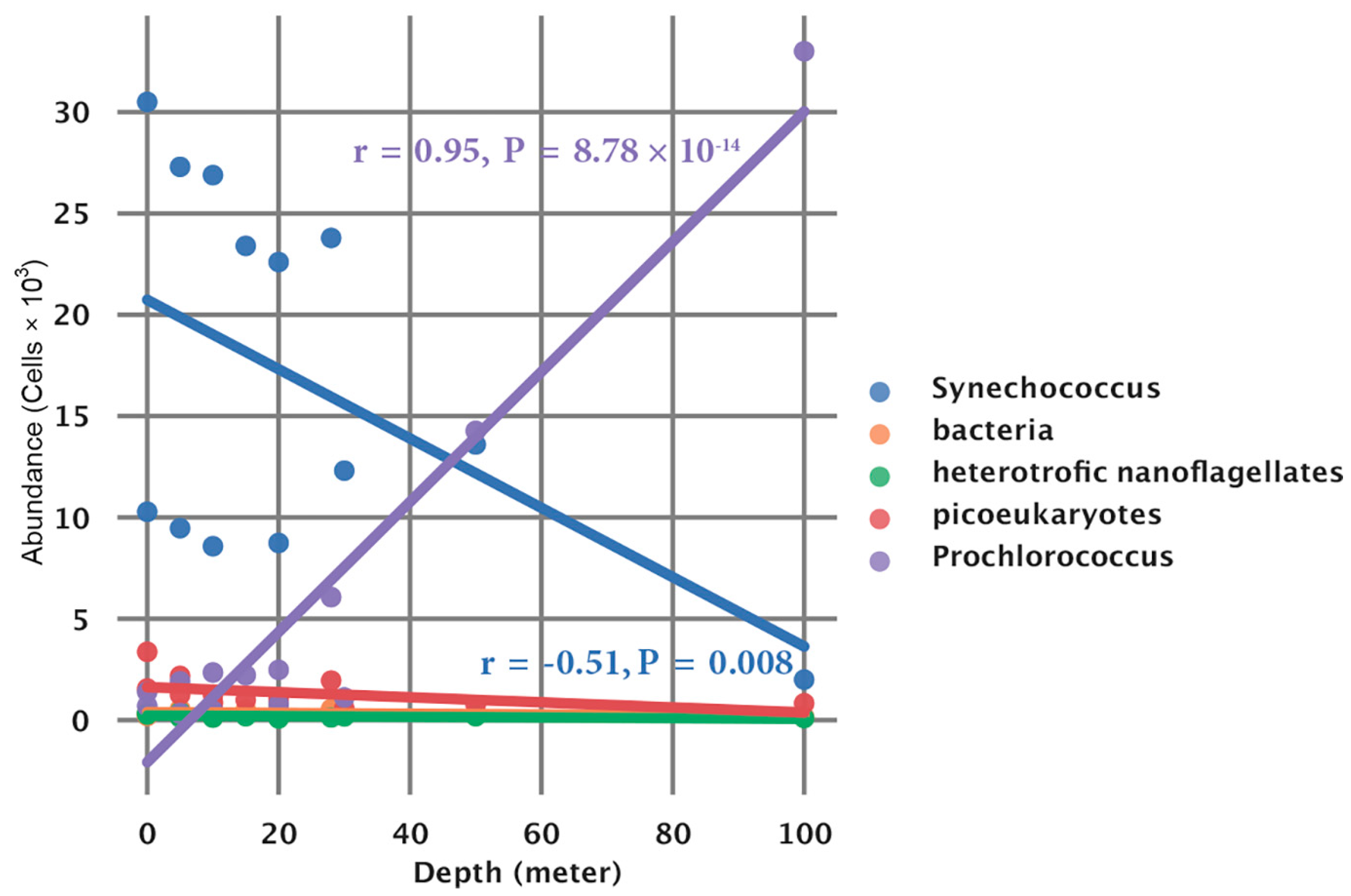
3.4. Microbial Community Structure at the Two Stations

We assessed the community structure and count of the microbial community with a flow cytometer and Utermöhl counting method [24]. Overall, the community is dominated by cyanobacteria Synechococcus (with concentrations ranging from 22.60 × 10³ to 30.50 × 10³ cells/mL at Kaštela and from 2.00 × 10³ to 13.60 × 10³ cells/mL at the Stončica-Vis location), with the highest concentrations at the surface decreasing with depth at Kaštela and the highest concentrations at 30 m and 50 m at the Stončica-Vis location. Cyanobacterium Prochlorococcus (with concentrations ranging from 1.39 × 10³ to 6.07 × 10³ cells/mL at Kaštela and from 0.70 × 10³ to 33.00 × 10³ cells/mL at the Stončica-Vis location) had the lowest concentrations at the surface, with increasing concentrations with depth, exhibiting dominant concentrations (14.27 × 10³ and 33.00 × 10³ cells/mL) at 50 m and 100 m, respectively, at the Stončica-Vis oligotrophic location. Picoeukaryotes concentrations generally decreased with depth, with a slight increase at 30 m at the Kaštela location (concentrations ranging from 0.86 × 10³ to 3.37 × 10³ cells/mL), and were higher at 0 m and 5 m than the rest of the water column, wherein the concentrations were uniform at the Stončica-Vis location (with concentrations ranging from 0.57 × 10³ to 1.56 × 10³ cells/mL). Concentrations of heterotrophic nanoflagellates were uniform throughout the water columns at both Kaštela and Stončica-Vis locations (with concentrations ranging from 0.13 × 10³ to 0.40 × 10³ cells/mL). Heterotrophic bacteria were the most dominant population within the microbial community at both locations, uniformly distributed throughout the water columns (with concentrations ranging from 0.31 × 10⁶ to 0.55 × 10⁶ cells/mL at Kaštela and 0.15 × 10⁶ to 0.30 × 10⁶ cells/mL at the Stončica-Vis location). The density and enrichment of Prochlorococcus, Synechococcus, and picoeukaryotes in the water column are shown in Figure A4.

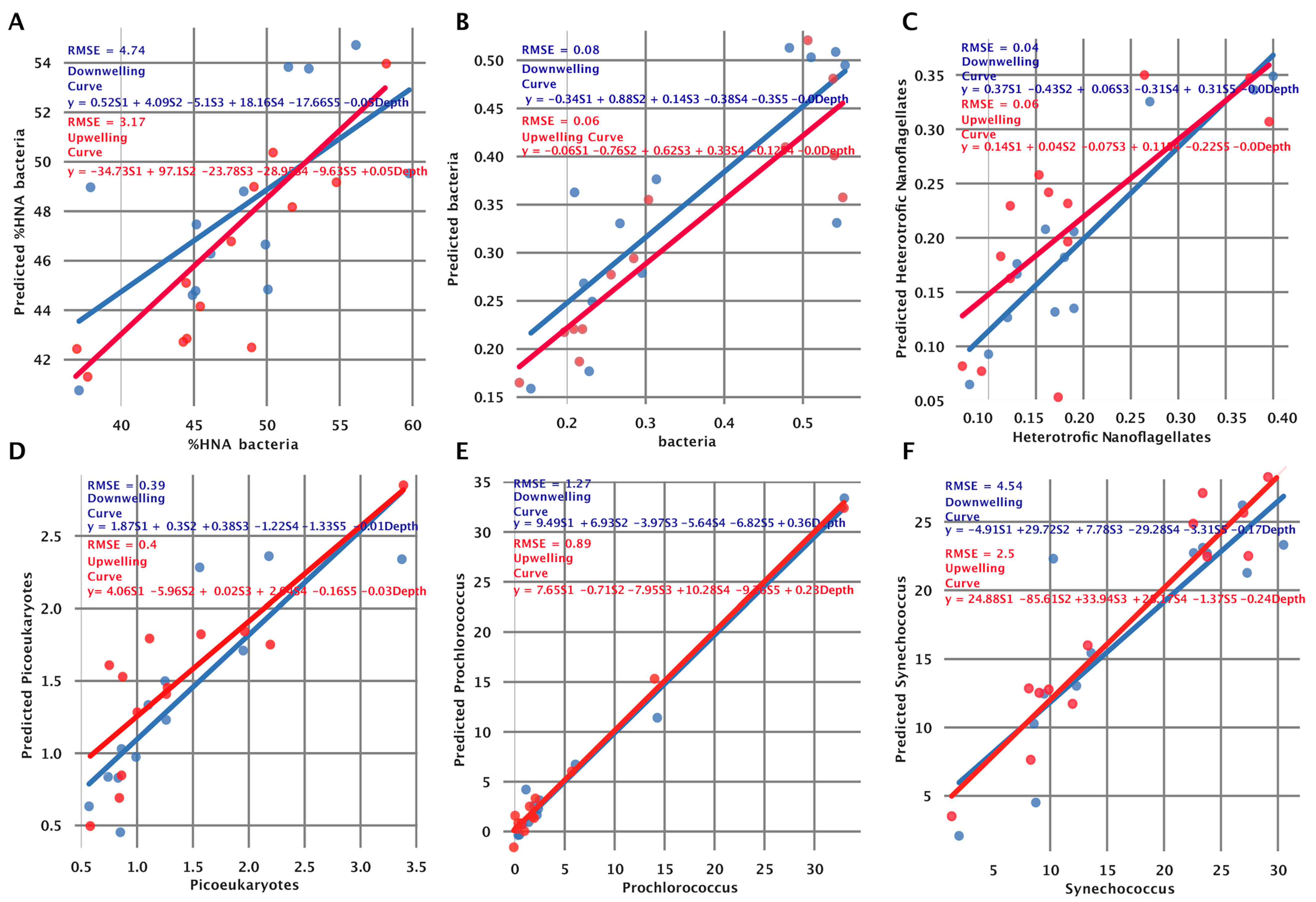
3.5. Fitting the Model to Independent Data Collected at the Two Stations

After model training, we used the trained NMF model on data obtained at Kaštela (K0, K5, K10, K15, K20, K25, K28) and Stončica-Vis (V0, V5, V10, V20, V30, V50, V100). First, we inspected the signature enrichment distribution between the two locations and two sensors (downwelling and upwelling). At the Kaštela Bay downwelling sensor (DW) (Figure 2A, left top), we observed a dominant presence of S1 and S3. S1 starts the highest and peaks at 0 m, peaks at 5 m, and slowly vanishes.

Furthermore, S1 was also correlated (r = 0.87, p < 0.001) to Synechococcus, heterotrophic nanoflagellates, and Picoeukaryotes counts (Figure 2B, Kaštela downwelling panel) and spectral peaks of 356 nm and 593 nm. Enrichment of S3 was expressed in two peaks, one at 5 m and another one at 28 m. Furthermore, S3 (curve peak at 496 nm) showed a significant positive correlation to Chlorophyll a and Prochlorococcus (r = 0.71, p < 0.001 and r = 0.72, p < 0.001) (Figure 2B, Kaštela downwelling panel). Signatures S2 and S5 showed similar patterns as they started with low values, peaked at 10 m, and decreased afterward. At the same location and in the upwelling sensor (UW) (Figure 2A, right top), we observed a dominant presence of S3 and S1 with limited enrichment of S4 at 5, 10, and 15 m. The signature S1 (curve peaks at 356 nm and 597 nm) is also correlated with Chlorophyll a, Prochlorococcus, and Picoeukaryotes (r = 0.48, p < 0.001; r = 0.38, p < 0.001; r = 0.57, p < 0.001) (Figure 2B, Kaštela upwelling panel), indicating different community structures at the surface compared to the lower parts of the water column. S1 (Chlorophyll a, Prochlorococcus, and Picoeukaryotes) showed the highest enrichment at 0 and 28 m and the lowest at 10 m. At the Stončica-Vis DW station, we observed almost no presence of S2 and some level of enrichment in other signatures. Signature S4 started with low values, peaked at 20 m, and decreased as depth increased. Signature S1 showed the highest enrichment at the surface and decreased as depth increased, except for 100 m (Figure 2A, Stončica-Vis DW panel). Signature S3 showed enrichment at all depths, reaching a maximum at 50 m. Looking at the UW sensor at the same location, we observed minimal or no presence of S4 except at 0 m and 30 m. Vertical distribution of microorganisms is under significant influence of moving masses of seawater, alongside the influence of nutrients and light [25,26]. Therefore, this could be the reason for difficulties in prediction of different groups of microorganisms within the marine water column. S4 was also characterized by a strong positive correlation (r = 0.48, p < 0.001; r = 0.6 p < 0.001) towards Chlorophyll a and Prochlorococcus (Figure 2B, Stončica-Vis UW panel). Signature S5 (wide curve with a peak in 446 nm) showed dominant enrichment peaking at 5 m and 20 m. Signature S3 showed maximum enrichment at 0 m and 30 m and a strong correlation (r = 0.79, p < 0.001; r = 0.72, p < 0.001; r = 0.81, p < 0.001) with Synechococcus, Bacteria, and Heterotrophic nanoflagellates (Figure 2B, Stončica-Vis UW panel). Next, we calculated and analyzed the Chlorophyll a absorbance for both stations (Kaštela and Stončica-Vis). At the Kaštela station, we observed the highest absorbance at 30 m and minimum absorbance at 5 m depth, whereas at Stončica-Vis station, the highest absorbance was measured at 0 m and minimum at 100 m depth (Figure 2C). Interestingly, the second highest chlorophyll absorbance at Stončica-Vis station was at 30 m depth, where absorbance in the spectrum of 400 to 500 nm exceeded the absorbance of 0 m. Furthermore, V30 is also characterized by enriched S4 (DW), which is characterized by a broad, low-intensity curve located between 353 and 503 nm and an increased concentration of Prochlorococcus.

Finally, we inspected the overall association of the count (10³ cell/mL) of members of the picoplankton community and depth. The Synechococcus count was significantly negatively correlated (r = -0.51, p = 0.008) with depth (m), and Prochlorococcus was significantly positively correlated (r = 0.95, p < 0.001) with depth (m) (Figure A2).

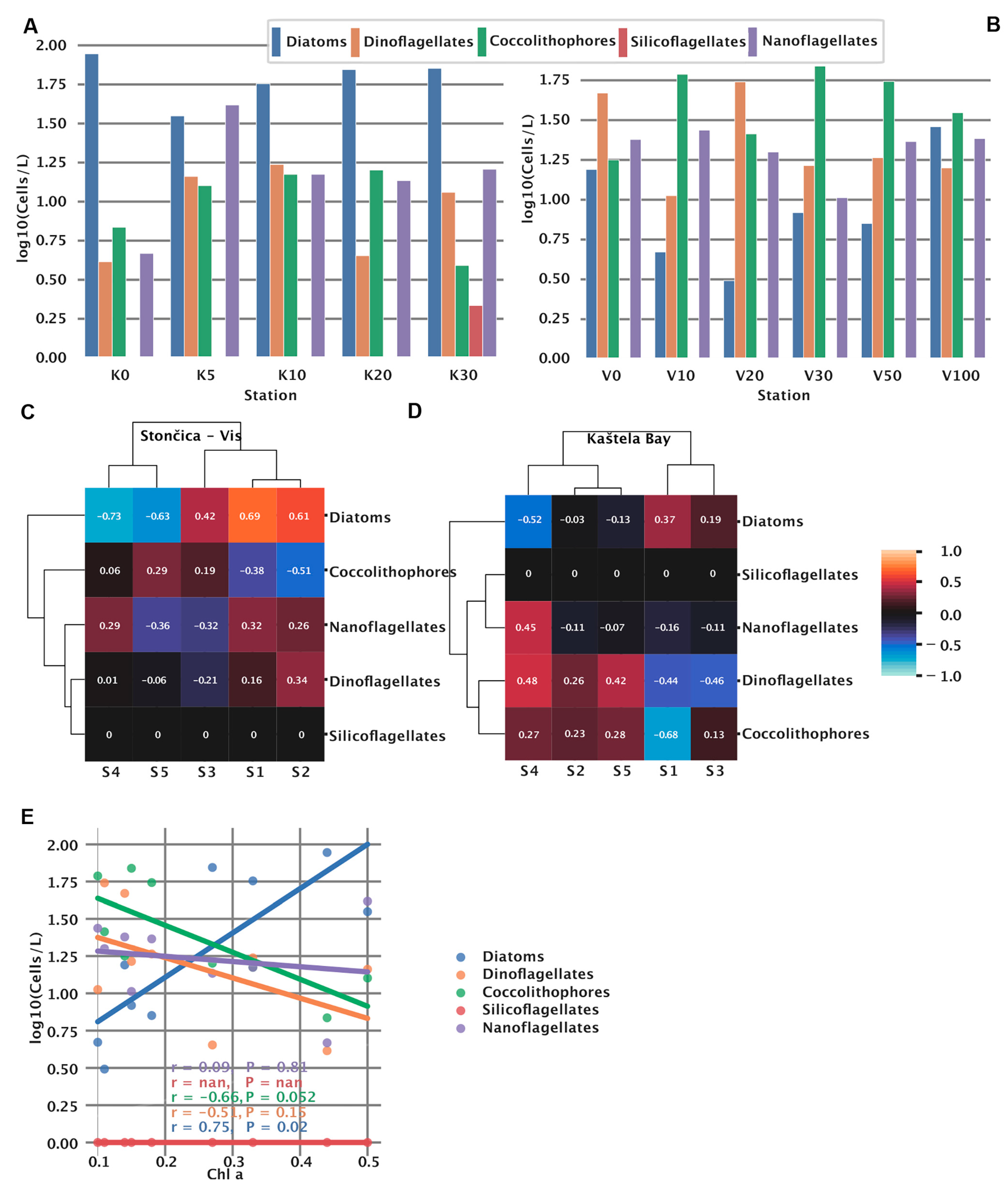
3.6. Phytoplankton Abundance and Community Structure

At both locations, phytoplankton abundance was measured to assess the community structure. Kaštela Bay water column was dominated by diatoms, having almost uniform and enriched abundance at all measured depths (0–30 m) (Figure 3A).

In contrast, silicoflagellates showed no presence at either stations except for Kaštela at 30 m. At Kaštela, the surface was largely dominated by diatoms, whereas at Stončica-Vis, dinoflagellates were the most abundant (Figure 3B). At Stončica-Vis, diatoms show an interesting pattern where they start at a high value at the surface, reaching a minimum at 20 m, and then steadily increase again, reaching a maximum at 100 m. The similar pattern we observed for S1 for both UW and DW sensors at Stončica-Vis (Figure 2a) suggests an association between diatom abundance and S1. To further investigate this, we correlated signatures to phytoplankton groups and observed positive correlations between S1 and diatoms for Stončica-Vis (Figure 3C and Figure A3). Furthermore, at Kaštela, nanoflagellates and S4 from the upwelling curve showed a similar pattern, reaching a maximum value at 5 m and slowly decreasing to 30 m (Figure 2a and Figure 3A). This was further confirmed by a correlation coefficient between S4 and nanoflagellates, suggesting a strong positive correlation (Figure 3D and Figure A3). In Kaštela, we also observed that the abundance of coccolithophores started with smaller values at the surface and increased until 10–20 m and then decreased, reaching a minimum at 30 m (Figure 3A). A similar pattern was observed for S5 (only DW) in Kaštela, where S5 enrichment peaked at 10 m (Figure 2a), suggesting an association between S5 (DW) and the abundance of coccolithophores (Figure A3). Performing hierarchical clustering (ward algorithm) on correlation coefficients between phytoplankton and signatures, we observed different community structures between Kaštela and Stončica-Vis. At the Stončica-Vis location, diatoms were strongly associated with S1 and S2 and negatively associated with S4 and S5 (Figure 3C). At Kaštela, diatoms showed an intermediate association with S1 and a strong negative association with S4 (Figure 3D). Lastly, we correlated Chlorophyll a with the abundance of phytoplankton groups. We observed a significant positive correlation between the abundance of diatoms and Chlorophyll a (r = 0.75 p = 0.02) and a marginally significant negative correlation (r = −0.66 p = 0.052) between coccolithophores and Chlorophyll a (Figure 3E).

Abundances and detailed species distribution per station per depth are shown in the Supplementary Data Files/Phytoplankton. We did not find any species-specific correlation with extracted signatures; therefore, in our analyses, we focused only on larger groups identified by light microscopy.

3.7. Spectral Signatures and Microbial Community Structure

The collected data for microbial community structure and HOCR can be paired by depth, which is ideal for modeling. For this purpose, we constructed simple linear regressions to predict count (10³ Cells/mL) using our signatures (S1–S5) and depth. For each microbial count, we made a model using extracted signatures from the upwelling curve and the downwelling curve. Next, we plotted the observed count (10³ Cells/mL) on the x axis and the predicted count (10³ Cells/mL) on the y axis. In the ideal case, those points would form a diagonal line representing no difference between observed and predicted values. This analysis showed that bacteria, heterotrophic nanoflagellates, and picoeukaryotes can be predicted using extracted signatures with minimal root mean square error (RMSE), where Prochlorococcus showed intermediate RMSE values and finally, Synechococcus and HNA bacteria showed large RMSE (Figure 4A–F). The corresponding coefficients on the linear regression line indicate the “importance” of each variable (S1–S5 and depth). Figure 4B showed a small RMSE, indicating a low error when predicting bacterial abundance, but also the largest coefficient associated with S2 and a coefficient of 0 associated with depth. This exploratory analysis indicated that the abundance of bacteria does not depend on depth, but on the light spectrum (and more specifically on the high-intensity broad light spectrum peak around 503 nm).

When predicting bacteria, we observed an RMSE of 0.08 when using a downwelling curve and RMSE = 0.06 when using an upwelling curve, indicating that bacterial count can be effectively estimated using our signatures. The coefficient associated with the depth is equal to zero, indicating that all information for prediction is coming from signatures, mainly from S2, when looking at the downwelling curve model (Figure 4B). Fitting a model that predicts the count of heterotrophic nanoflagellates showed the best results in terms of RMSE. We calculated an RMSE of 0.04 when using the downwelling curve and an RMSE of = 0.06 when using the upwelling curve (Figure 4C). The model that predicts Picoeukaryotes showed an RMSE of 0.39 when using signatures from the downwelling curve and an RMSE of 0.40 when using signatures from the upwelling curve. The coefficient of 0.03 associated with depth signifies a marginal correlation between depth and count, as illustrated in Figure 4D. Fitting a model that predicts the count of Prochlorococcus, we observed an RMSE of 1.27 when using signatures extracted from the downwelling curve and an RMSE of 0.89 when using signatures extracted from the upwelling curve. We noted a positive coefficient (0.36 for downwelling and 0.23 for upwelling) associated with depth (Figure 4E), aligning with the earlier discovery of a comprehensive positive correlation between Prochlorococcus count and depth (r = 0.95 p < 0.001, Figure A2). The model that predicts the count of Synechococcus achieved poor results in terms of RMSE. When using extracted signatures from the downwelling and upwelling curves, we calculated an RMSE of 4.54 and an RMSE of 2.50, respectively (Figure 4F). Interestingly, coefficients associated with signatures vary when using downwelling and upwelling curves for signature extraction but also when comparing different species. In Kaštela, when using downwelling sensor signatures, we observed that heterotrophic nanoflagellates were strongly correlated with S1 (characterized by HOCR peaks at 363 nm and 583 nm), which was enriched at 0 m and 5 m depths (Figure 2B). In Stončica-Vis, when using an upwelling curve for signature extraction, we observed that the count of bacteria was strongly correlated with S3, which is characterized by a small peak at 483 nm in an HOCR curve. When looking at the S3 enrichment (Figure 2A, Stončica-Vis UW), we observed that S3 showed high enrichment at a depth of zero; minimal enrichment at 5 m, 10 m, and 20 m depths; and high enrichment again at 30 m and 50 m depth, indicating a complex structure of the microbial community and their interaction with the light spectrum.

4. Discussion

The outcomes of our study underscore the potential of AI to enhance predictive modeling in ecological studies. The nuanced RMSE values reveal the intricacies of microbial predictions, encouraging further exploration into refining ML algorithms for more accurate ecological assessments. The integration of ML and AI components, particularly the NMF model, emerges as a transformative approach for real-time, detailed analysis of ocean water columns. The correlation between spectral signatures and microbial abundances highlights the potential of ML in advancing our understanding of ocean ecosystems. Our results pave the way for a paradigm shift, where sensor systems coupled with AI frameworks enable comprehensive oceanographic analyses without the traditional reliance on water samples.

Measurements of samples taken at specific depths and the extracted signatures provide comprehensive results. Combining all the approaches described above, our results clearly show a significant relationship between the microbial community, photosynthetic and heterotrophic activity, and downwelling and upwelling radiation intensity in the water column. Downwelling irradiance spectra represent adsorption of spectra through the water column by the seawater, inorganic particles, and microbial consortia, while upwelling spectra represent the reflection of spectra from different particles below the upwelling sensor.

Our extracted spectral signatures can accurately predict the numbers of bacteria, heterotrophic nanoflagellates, and picoeukaryotes. Cyanobacteria (both Prochlorococcus and Syechococcus) are poorly predictable from our signatures (being only associated with depth). Heterotrophic nanoflagellates are also very poorly predictable regardless of depth (Figure 4). As we reflect on the implications of our findings, the role of AI in shaping the future of oceanography becomes increasingly evident. The marriage of advanced sensors and ML models not only expedites data analysis but also opens avenues for continuous, real-time monitoring of oceanic dynamics, ushering in a new era of AI-driven environmental science. The process of predicting phytoplankton concentrations from measured HOCR spectra is shown in a flow diagram in Figure A5. Prochlorococcus and Synechococcus are widely distributed across the world’s oceans and coexist in marine environments. The abundances of Prochlorococcus and Synechococcus in the Mediterranean are like those in the Adriatic, with maximum abundances of Prochlorococcus in the subsurface layer [27].

The main taxonomic groups of eukaryotic phytoplankton are also widespread in all oceans, and the contribution of diatoms and dinoflagellates in coastal and open waters is like that in the Mediterranean. The dynamics of environmental parameters play a central role in determining the succession and diversity of phytoplankton communities. For example, small dinoflagellates, which are characteristic of oligotrophic areas, predominate in open areas (Vis-Stončica), while diatoms are more common in neritic areas (Kaštela Bay), which is also characteristic of the Mediterranean [28].

Analysis of satellite images of ocean color in the Mediterranean Sea identified dominant phytoplankton groups such as nanoeukaryotes, Prochlorococcus, Synechococcus, diatoms, Phaeocystis-like, and coccolithophores [28,29]. The following main functional groups of phytoplankton were quantified in surface samples along a transect in the Atlantic Ocean: Prochlorococcus, Synechococcus, coccolithophores, nanoeukaryotes, diatoms and dinoflagellates [30].

The Middle Adriatic Sea is generally considered as an oligotrophic (low-production) ecosystem in which picophytoplankton accounts for a large portion of the total plankton biomass [31,32]. Our results fit well into that consideration, indicating a significant role of picoplankton size fraction in the microbial food web. Thermohaline circulation in this area shows pronounced stratification of the water column from June to September, when advective movement of water masses and turbulent mixing is significant; it was noted that it has weakened because of global warming [33], which may have significant impact on the availability of nutrients and thus the functioning of the microbial food web. Our measurements indicate that we conducted our experiment at the beginning of the stratification period (Figure A1), which might influence the accuracy of prediction of different groups of microorganisms.

Abundances and detailed species distribution per station per depth are shown in the Supplementary Data File/Phytoplankton. We did not find any species-specific correlation of species identified by light microscopy with extracted signatures; therefore, in our analyses, we focused only on larger groups of organisms. We believe a different approach should be used in future validations; alongside light microscopy, the application of 16S/18S/ITS amplicon sequencing protocols (or similar) may be a good idea for the main purpose of refining and standardizing predictions and comparisons with other areas/studies. Within the wider context of our project’s primary goal, our results indicate that the vertical distribution of microorganisms is under significant influence of moving masses of seawater alongside the influence of nutrients and light [25,26]. As we indicated significant contribution and specific density and enrichment of picophytoplankton to the microbial community within the water column at our study sites, it could be postulated that they are an important source of colored dissolved organic matter, as previously found in the warming waters of the North Atlantic [34].

We have shown that HOCR-extracted spectral signatures can be used to predict the structure of different groups of organisms that make up the microbial community. Using extracted spectral signatures in a simple linear model, we showed that Prochlorococcus abundance could be predicted with intermediate RMSE values. Synechococcus and HNA bacteria showed a large RMSE, indicating poor predictive power and marginal association with the light spectrum. Finally, the abundances of bacteria, heterotrophic nanoflagellates, and picoeukaryotes could be predicted with minimal RMSE, indicating association with our extracted light spectrum signatures. Our results opened a clear pathway towards the concept of detailed and comprehensive analysis of the ocean water column (from macro to nanometer scale) in real time, using solely sensor systems coupled with an AI data analysis framework, without the necessity of taking seawater samples with bottles.

From the perspective of the NMF model, the entire experiment conducted at the Stončica-Vis and Kaštela-Bay locations is a validation of the model and proof that we can use it on other sites. The main advantage of ML and AI in such systems is that models with powerful predictive power can replace the need for expensive on-site laboratories for microenvironment characterization. Sensor systems are more convenient to deploy as they can collect data that can be analyzed. For example, our NMF model outputs five distinct signatures, where each one of them represents a specific spectrum of light and a specific association with cell abundance.

It is important to note that this is the first attempt to use this approach in the prediction of microbial groups in the marine water column. Future applications of the proposed approach should include measurements in different marine environments accompanied by other contemporary biodiversity methods to create a large enough database to achieve the goal of microbial community analysis without the necessity of taking physical samples of seawater.

References

1. Bukata, R.P.; Jerome, J.H.; Kondratyev, A.S.; Pozdnyakov, D.V. Optical Properties and Remote Sensing of Inland and Coastal Waters, 1st ed.; CRC Press: Boca Raton, FL, USA, 1995. [Google Scholar]
2. Feng, H.; Campbell, J.W.; Dowell, M.D.; Moore, T.S. Modeling spectral reflectance of optically complex waters using bio-optical measurements from Tokyo Bay. Remote Sens. Environ. 2005, 99, 232–243. [Google Scholar] [CrossRef]
3. IOCCG. Remote Sensing of Inherent Optical Properties: Fundamentals, Tests of Algorithms, and Applications; Lee, Z.-P., Ed.; Reports of the International Ocean-Colour Coordinating Group; International Ocean-Colour Coordinating Group (IOCCG): Dartmouth, NS, Canada, 2006; pp. 1–122. [Google Scholar]
4. Strömbeck, N.; Pierson, D.C. The effects of variability in the inherent optical properties on estimations of chlorophyll a by remote sensing in Swedish freshwaters. Sci. Total Environ. 2001, 268, 123–137. [Google Scholar] [CrossRef] [PubMed]
5. Cullen, J.J.; Ciotti, Á.M.; Davis, R.F.; Lewis, M.R. Optical detection and assessment of algal blooms. Limnol. Oceanogr. 1997, 42, 1223–1239. [Google Scholar] [CrossRef]
6. Schofield, O.; Grzymski, J.; Bissett, W.P.; Kirkpatrick, G.J.; Millie, D.F.; Moline, M.; Roesler, C.S. Optical monitoring and forecasting systems for harmful algal blooms: Possibility or pipe dream? J. Phycol. 1999, 35, 1477–1496. [Google Scholar] [CrossRef]
7. IOCCG. Phytoplankton Functional Types from Space; Sathyendranath, S., Ed.; Reports of the International Ocean-Colour Coordinating Group; International Ocean-Colour Coordinating Group (IOCCG): Dartmouth, NS, Canada, 2014; pp. 1–154. [Google Scholar]
8. Mouw, C.B.; Hardman-Mountford, N.J.; Alvain, S.; Bracher, A.; Brewin, R.J.W.; Bricaud, A.; Ciotti, A.M.; Devred, E.; Fujiwara, A.; Hirata, T.; et al. A Consumer’s Guide to Satellite Remote Sensing of Multiple Phytoplankton Groups in the Global Ocean. Front. Mar. Sci. 2017, 4, 41. [Google Scholar] [CrossRef]
9. Ciotti, Á.M.; Lewis, M.R.; Cullen, J.J. Assessment of the relationships between dominant cell size in natural phytoplankton communities and the spectral shape of the absorption coefficient. Limnol. Oceanogr. 2002, 47, 404–417. [Google Scholar] [CrossRef]
10. Sathyendranath, S.; Lazzara, L.; Prieur, L. Variations in the spectral values of specific absorption of phytoplankton. Limnol. Oceanogr. 1987, 32, 403–415. [Google Scholar] [CrossRef]
11. Bricaud, A.; Claustre, H.; Ras, J.; Oubelkheir, K. Natural variability of phytoplanktonic absorption in oceanic waters: Influence of the size structure of algal populations. J. Geophys. Res. Ocean. 2004, 109, C11010. [Google Scholar] [CrossRef]
12. Jemai, A.; Wollschläger, J.; Voβ, D.; Zielinski, O. Radiometry on Argo Floats: From the Multispectral State-of-the-Art on the Step to Hyperspectral Technology. Front. Mar. Sci. 2021, 8, 676537. [Google Scholar] [CrossRef]
13. Wang, Y.-X.; Zhang, Y.-J. Nonnegative Matrix Factorization: A Comprehensive Review. IEEE Trans. Knowl. Data Eng. 2013, 25, 1336–1353. [Google Scholar] [CrossRef]
14. Pauca, V.P.; Piper, J.; Plemmons, R.J. Nonnegative matrix factorization for spectral data analysis. Linear. Algebra Appl. 2006, 416, 29–47. [Google Scholar] [CrossRef]
15. Alexandrov, L.B.; Nik-Zainal, S.; Wedge, D.C.; Campbell, P.J.; Stratton, M.R. Deciphering signatures of mutational processes operative in human cancer. Cell Rep. 2013, 3, 246–259. [Google Scholar] [CrossRef]
16. Marinov, I.; Doney, S.C.; Lima, I.D. Response of ocean phytoplankton community structure to climate change over the 21st century: Partitioning the effects of nutrients, temperature and light. Biogeosciences 2010, 7, 3941–3959. [Google Scholar] [CrossRef]
17. Puškarić, S.; Sokač, M.; Matić, K. Application of non-negative matrix factorization for studying short-term physiological changes in grapevine from canopy hyperspectral reflection. RIThink 2021, 10, 1–25. [Google Scholar]
18. Holm-Hansen, O.; Lorenzen, C.J.; Holmes, R.W.; Strickland, J.D.H. Fluorometric Determination of Chlorophyll. ICES J. Mar. Sci. 1965, 30, 3–15. [Google Scholar] [CrossRef]
19. Gasol, J.M.; Morán, X.A.G. Flow Cytometric Determination of Microbial Abundances and Its Use to Obtain Indices of Community Structure and Relative Activity. In Hydrocarbon and Lipid Microbiology Protocols; Springer: Berlin/Heidelberg, Germany, 2015; pp. 159–187. [Google Scholar]
20. Utermöhl, H. Zur Vervollkommnung der quantitativen Phytoplankton-Methodik. Mitt. Int. Ver. Theor. Angew. Limnol. 1958, 9, 1–38. [Google Scholar] [CrossRef]
21. Marasović, I.; Gačić, M.; Kovačević, V.; Krstulović, N.; Kušpilić, G.; Pucher-Petković, T.; Odzak, N.; Solic, M. Development of the red tide in the Kaštela Bay (Adriatic Sea). Mar. Chem. 1991, 32, 375–387. [Google Scholar] [CrossRef]
22. Lee, D.D.; Seung, H.S. Learning the parts of objects by non-negative matrix factorization. Nature 1999, 401, 788–791. [Google Scholar] [CrossRef] [PubMed]
23. Lancaster, P.; Tismenetsky, M. The Theory of Matrices: With Applications; Elsevier: Gainesville, FL, USA, 1985. [Google Scholar]
24. Paxinos, R. A rapid Utermohl method for estimating algal numbers. J. Plankton. Res. 2000, 22, 2255–2262. [Google Scholar] [CrossRef]
25. Vilibić, I.; Šantić, D. Deep water ventilation traced by Synechococcus cyanobacteria. Ocean Dyn. 2008, 58, 119–125. [Google Scholar] [CrossRef]
26. Šantić, D.; Kovačević, V.; Bensi, M.; Giani, M.; Vrdoljak Tomaš, A.; Ordulj, M.; Santinelli, C.; Šestanović, S.; Šolić, M.; Grbec, B. Picoplankton Distribution and Activity in the Deep Waters of the Southern Adriatic Sea. Water 2019, 11, 1655. [Google Scholar] [CrossRef]
27. Mella-Flores, D.; Mazard, S.; Humily, F.; Partensky, F.; Mahé, F.; Bariat, L.; Courties, C.; Marie, D.; Ras, J.; Mauriac, R.; et al. Is the distribution of Prochlorococcus and Synechococcus ecotypes in the Mediterranean Sea affected by global warming? Biogeosciences 2011, 8, 2785–2804. [Google Scholar] [CrossRef]
28. Aktan, Y. Large-scale patterns in summer surface water phytoplankton (except picophytoplankton) in the Eastern Mediterranean. Estuar. Coast Shelf. Sci. 2011, 91, 551–558. [Google Scholar] [CrossRef]
29. Navarro, G.; Alvain, S.; Vantrepotte, V.; Huertas, I.E. Identification of dominant phytoplankton functional types in the Mediterranean Sea based on a regionalized remote sensing approach. Remote Sens. Environ. 2014, 152, 557–575. [Google Scholar] [CrossRef]
30. Brotas, V.; Tarran, G.A.; Veloso, V.; Brewin, R.J.W.; Woodward, E.M.S.; Airs, R.; Beltran, C.; Ferreira, A.; Groom, S.B. Complementary approaches to assess phytoplankton groups and size classes on a long transect in the Atlantic Ocean. Front. Mar. Sci. 2022, 8, 682621. [Google Scholar] [CrossRef]
31. Šolić, M.; Šantić, D.; Šestanović, S.; Bojanić, N.; Grbec, B.; Jozić, S.; Vrdoljak, A.; Ordulj, M.; Matić, F.; Kušpilić, G.; et al. Impact of water column stability dynamics on the succession of plankton food web types in the offshore area of the Adriatic Sea. J. Sea Res. 2020, 158, 101860. [Google Scholar] [CrossRef]
32. Šantić, D.; Krstulović, N.; Šolić, M.; Ordulj, M.; Kušpilić, G. Dynamics of prokaryotic picoplankton community in the central and southern Adriatic Sea (Croatia). Helgol. Mar. Res. 2012, 67, 471–481. [Google Scholar] [CrossRef]
33. Vilibić, I.; Šepić, J.; Proust, N. Weakening thermohaline circulation in the Adriatic Sea. Clim. Res. 2013, 55, 217–225. [Google Scholar] [CrossRef]
34. Organelli, E.; Claustre, H. Small Phytoplankton Shapes Colored Dissolved Organic Matter Dynamics in the North Atlantic Subtropical Gyre. Geophys. Res. Lett. 2019, 46, 12183–12191. [Google Scholar] [CrossRef]
Figure 1. Signature development using training data. (a) In order to find the optimal number of signatures (K), we computed two measurements (Frobenius norm and Kullbeck–Leibler), for every K in the range of two to ten. This analysis showed that K = 5 is the optimal number of signatures. (b) Each signature can be visualized as a spectral curve indicating distinct patterns in data. (c) Signatures were made using data collected from two sensors, upwelling (UW) and downwelling (DW). The two sensors show distinct enrichment of signatures. (dh) To investigate the association between depth and each signature, we computed the kernel density estimation (KDE). This analysis showed that some signatures are present at all depths (S1, S3, S5) while others are present mostly around the surface (S2 and S4).
Jmse 12 00286 g001
Figure 2. NMF application of HOCR curves collected at two locations. (A) A trained NMF model was applied to data at collected Kaštela Bay and Stončica-Vis. The bar plot shows the enrichment of each signature for each measurement. For this study, we used only one sample per depth. (B) The heatmap shows correlation coefficients between signature enrichment and abundance of cyanobacteria, heterotrophic bacteria, heterotrophic nanoflagellates, picoeukaryotes, and Chlorophyll a for both locations and both sensors. (C) The line plot shows absorption of Chlorophyll a within the spectrum of 300 nm and 900 nm. The colors indicate the depth at which the sample was collected.
Jmse 12 00286 g002
Figure 3. Phytoplankton significance at two study locations. (A) Phytoplankton abundance at the Kaštela Bay and (B) Stončica-Vis study sites. For the purpose of this study, we used only one sample per depth. Heatmaps (C,D) showing a correlation between different phytoplankton taxa and extracted spectral signatures at the (C) Kaštela Bay and (D) Stončica-Vis study sites. Correlations of phytoplankton taxa with Chlorophyll a (E).
Jmse 12 00286 g003
Figure 4. Linear regression models for prediction of phytoplankton and cyanobacteria abundance. (A) %HNA bacteria, (B) bacteria, (C) heterotrophic nanoflagellates, (D) picoeukaryotes, (E) Prochlorococcus, and (F) Synechococcus. The points represent the true value of abundance (x axis) and the predicted value of abundance (y axis), not the linear regression line. In the ideal case, this would be a clear diagonal line, indicating the perfect fit. The performance of the model is stated for each subpanel with root mean square error metric (RMSE) alongside the definition of a model (formula). Using the formula, readers can see which signatures are contributing to the prediction of abundance. Those models are fitted using a small amount of data, and they are for exploratory purposes. In other words, we wanted to test which microbial abundance groups we could predict and which ones we could not. This tells us if abundances are associated with extracted signatures (light spectrum), depth, or both.
Jmse 12 00286 g004