Numerical Simulation and Design of a Shaftless Hollow Pump for Plankton Sampling

Abstract

It is important to marine ecology research that plankton samples are collected without damage, especially for time series samples. Usually, most fixed-point plankton samplers are made using a pump with paddle blades in order to increase the flow rate. But it can easily injure soft plankton. In this paper, a shaftless hollow sampling pump is designed, which can provide a highly efficient driving component for the plankton sampler. The numerical model of the sampling pump is established, and the flow rate of the sampling pump at different rotational speeds is simulated by the computational fluid dynamics method. In order to obtain a higher flow rate, the influence of internal and external cavity size, blade angle, and blade number on the flow rate of the sampling pump with a constant rotational speed of the blade was simulated and discussed. The results show that the flow rate at the internal cavity is positively correlated with the inlet and outlet pressure differences of the internal cavity, and the greater the negative pressure at the outlet of the internal cavity, the greater the flow rate. When the internal and external cavity sizes are h = 14 mm, d = 52 mm, blade angle θ = 45°, and number of blades s = 5, the flow rate of the sampling pump internal cavity reaches the maximum. Finally, the feasibility of the shaftless hollow sampling pump is verified by experiments. The shaftless hollow sampling pump can realize non-destructive sampling of plankton. This paper presents a theoretical design foundation for a new non-destructive siphon sampling method for marine plankton, which is of great significance for marine plankton sampling and subsequent research.

1. Introduction

Plankton is one of the key links in the food web and occupies an important niche in the marine ecosystem [1,2]. Efficient and non-destructive acquisition of marine plankton samples is a necessary means for scientists to carry out ecological research [3]. Trawl nets are commonly used to collect plankton samples, but they can only collect mixed samples within a section of water, making it difficult to carry out detailed studies, such as the diurnal migration process of zooplankton. Although stratified trawls such as ORI-VMPS [4], MOCNESS [5], and Multinet [6] are designed for fractional sampling in vertical profiles, it is difficult to obtain plankton samples for time series due to their reliance on survey ship operations [7].

The fixed-point sampler is a kind of plankton sampling device driven by seawater filtration through pumps. It is small in size, low cost, and can be conveniently deployed on buoys [8]. With programming control, plankton samples of time series can be obtained periodically to study the periodic changes of plankton. It can also be carried on an underwater vehicle to obtain samples at a specified location.

Plankton pumps produced by KC Denmark, which are filtered by a top motor pushing water flow, have been used for plankton collection in Brest and Sardinia bays [9,10]. The plankton pump designed by Wilborn was used to collect large and medium-sized plankton on the benthos. The Blue Robotics T200 propeller was used to directly drive the water flow to take samples so that the samples were sucked into the pre-collection net, and samples were obtained in the western Gulf of Alaska [11]. Billings designed the SyPRID sampler, where a large axial flow pump is placed behind the filter to form a sampling pump, which is used to collect plankton samples in a large volume of water with a flow rate of 700 m³/h [12].

In deeper waters, where plankton numbers are lower, large amounts of water must be filtered to obtain accurate statistics. The pump that drives the water flow is the key component of the fixed-point plankton sampler. In order to obtain a large flow rate, the propeller axial flow pump or centrifugal pump is usually designed. The pump can be installed in front of the filter and back of the filter in two ways. The disadvantage of front-mounted pumps is that the blades rotate at high speed, breaking up plankton with softer body tissues. Rear-mounted pumps can lead to a blockage of the collection net and a reduction in water flow, as well as the crushing of plankton samples. Therefore, fixed-point sampling pumps have not been well used in plankton surveys.

Computational fluid dynamics (CFD) has played a significant role in fluid machinery [13]. The use of CFD in fluid machinery design can provide a clear understanding of the flow field characteristics inside the machinery and optimize the design based on the flow field characteristics and design requirements [14]. LES, RANS, and hybrid RANS-LES models are commonly used in turbulence numerical simulation application research. The RANS model can simulate turbulent states with complex geometric shapes, but it is not suitable for separated flows. LES can effectively improve the defects of RANS, but the high grid quality requirements of LES near the wall result in high computational costs [15]. Currently, RANS is the most widely used turbulence numerical simulation method [16], and the RANS model includes k-ε and the k-$\omega$ model, where k-ε mainly includes Standard k-ε, Realizable k-ε, and RNG [17,18,19], k-$\omega$ mainly includes k-$\omega$ and SST k-$\omega$ [20,21]. De Donno designed a cooling centrifugal pump for automotive engines using the RANS model, reducing the load on the blades and improving pump efficiency [22,23]. Rong Guo studied the factors affecting centrifugal pump efficiency using the RANS model and found that various distortion conditions in centrifugal pumps can affect pump performance and stability [24].

In order to obtain non-destructive sampling of plankton under large flow, a shaftless hollow pump based on the Bernoulli principle is proposed. High-velocity fluid is used to create a pressure difference to push the injection flow so that plankton does not touch the paddle during the process of entering the sampler. In this paper, COMSOL (6.0) numerical simulation software is used to research the feasibility of using the water pressure difference generated by high-speed flow to absorb water samples and the influence of the internal and external cavity size, blade angle, and number of blades on the flow rate of the shaftless hollow pump is analyzed so as to achieve a better design. The prototype of a shaftless hollow pump is developed, and the experimental platform is set up to verify its feasibility.

2. Design Principles

The working principle of the shaftless hollow sampling pump is shown in Figure 1. Under the kinetic energy provided by the external cavity blade (“3”), high-speed water flow is generated and flows into the external pipe (“9”). Under the action of viscous force, the velocity and pressure gradually decrease along the flow direction behind the blade until the outlet of the pipe (“10”). The inlet of the internal and external cavities (“1,2”) and the outlet of the pipe are connected to the outside, and the pressure is environmental pressure. The high-speed water flow in the external cavity (“4”) joins together with the flow from the internal cavity (“6”) at the external cavity outlet (“7”) and the internal cavity outlet (“8”). As a result, the water flow velocity from the internal cavity increases under the action of viscous force. According to Bernoulli’s principle, the kinetic energy at the internal cavity outlet increases, the pressure potential energy decreases, and the pressure at the internal cavity outlet is lower than that at the inlet, forming a negative pressure and driving the fluid in the internal cavity continue to flow along the streamwise direction. After that, under the action of inertial force and viscous force, the fluid continues to flow along the streamwise direction to the outlet of the pipe; the speed gradually decreases, and the pressure gradually rises to the environmental pressure at the outlet. Because the blades are located in the external cavity, the sample is sucked along with the flow of the internal cavity without touching the blade, which ensures the integrity of the biological sample and thus realizes non-axial hollow sampling.

3. Sample Pump Numerical Model

COMSOL Multiphysics (6.0) is a multi-physics simulation software. In this paper, the CFD module of COMSOL Multiphysics is applied to establish a three-dimensional model for numerical simulation analysis and discussion of flow fields.

3.1. Governing Equations and Turbulence Models

The volume flow rate is calculated as follows:

$$Q=〈V〉·S$$

(1)

where $Q$ is the volume flow rate, $〈V〉$ is the area-weighted average velocity along the normal direction at the cross-section of the fluid flow, and $S$ is the cross-sectional area.

The type of flow field is determined by the dimensionless Reynolds number, which is the ratio relationship between two forces in a fluid (inertial force and viscous force), as follows:

$$Re=\frac{\rho 〈V〉L}{\mu }$$

(2)

where $\rho$ is the fluid density, $L$ is the characteristic length, and $\mu$ is the dynamic viscosity of the fluid.

Based on the design suction flow rate of 1 m³/h, the Reynolds number can be calculated to be about 5982, and the rotating water is more consistent with the turbulent state, so the flow is turbulent. Among the numerous turbulence models, Realizable k-ε turbulence model is widely used and is suitable for flow in rotating zones, with high accuracy and good turbulence consistency in circular tube jets [25,26,27]. Therefore, in this paper, Realizable k-ε turbulence model is adopted to analyze the flow field distribution in the shaftless hollow pump. The mass continuity equation and momentum equation [28] are as follows:

$$\frac{\partial \rho }{\partial t}+\frac{\partial \rho u_i}{\partial x_i}=0$$

(3)

$$\frac{\partial \rho u_i}{\partial t}+\frac{\partial \rho u_i{u}_j}{\partial x_j}=-\frac{\partial p}{\partial x_i}+\frac{\partial {\tau }_{ij}}{\partial x_j}+\frac{\partial }{\partial x_j}\left({\mu }_t\left(\frac{\partial u_i}{\partial x_j}+\frac{\partial u_j}{\partial x_i}\right)-\frac{2}{3}{\delta }_{ij}\left(\rho k+{\mu }_t\frac{\partial u_k}{\partial x_k}\right)\right)$$

(4)

where $t$ is the time, $x_i$ is the coordinate of the space cartesian coordinate system, $\rho$ is the liquid density, $u_i$ is the average velocity component, $p$ is the pressure, ${\tau }_{ij}$ is the strain rate tensor, and ${\mu }_t$ is the turbulent eddy viscosity.

Realizable k-ε turbulence equation is as follows:

$$\frac{\partial }{\partial t}\left(\rho k\right)+\frac{\partial }{\partial x_j}\left(\rho k{u}_j\right)=\frac{\partial }{\partial x_j}\left[\left(\mu +\frac{{\mu }_t}{{\sigma }_k}\right)\frac{\partial k}{\partial x_j}\right]+G_k+G_b-\mathsf{\rho }\mathsf{\epsilon }$$

(5)

$$\frac{\partial \rho \epsilon }{\partial t}+\frac{\partial \rho \epsilon u_j}{\partial x_j}=\frac{\partial }{\partial x_j}\left[\left(\mu +\frac{{\mu }_t}{{\sigma }_{\epsilon }}\right)\frac{\partial \epsilon }{\partial x_j}\right]+\rho C_{1}S\epsilon -\rho C_2\frac{{\epsilon }^2}{k+\sqrt{v\epsilon }}$$

(6)

where ${\mu }_t=\rho C_{\mu }\frac{k^2}{\epsilon }$, $C_1=\mathrm{m}\mathrm{a}\mathrm{x}[0.43,\frac{\eta }{\eta +5}]$, $C_2=1.9$, $\eta =S\frac{k}{\epsilon }$, $S=\sqrt{2S_{ij}{S}_{ij}}$, $S_{ij}=\frac{1}{2}\left(\frac{\partial u_i}{\partial x_j}+\frac{\partial u_j}{\partial x_i}\right)$, $G_k$ is the average velocity gradient, ${\sigma }_k$ is the Prandtl number of turbulent flow energy, ${\sigma }_{\epsilon }$ is the turbulent dissipation rate Prandtl number, $v$ is the fluid motion viscosity.

The calculation formulas for the momentum equation, k and ε in the wall function are:

$$u^{+}=\frac{1}{\kappa }\ln \left(E{y}^{+}\right)$$

(7)

$$G_k\approx {\tau }_w\frac{\partial u}{\partial y}={\tau }_w\frac{{\tau }_w}{\kappa \rho C_{\mu }^{1/4}{k}_P^{1/2}∆y_P}$$

(8)

$$\epsilon =\frac{C_{\mu }^{3/4}{k}_P^{3/2}}{\kappa ∆y_P}$$

(9)

where $y^{+}=\frac{∆y_P\left(C_{\mu }^{1/4}{k}_P^{1/2}\right)}{\mu },$ $\kappa =0.4,$ $E=0.8,$ $∆y_P$ is the distance from the node to the wall, $\mu$ is the fluid dynamic viscosity, ${\tau }_w$ is the wall shear stress.

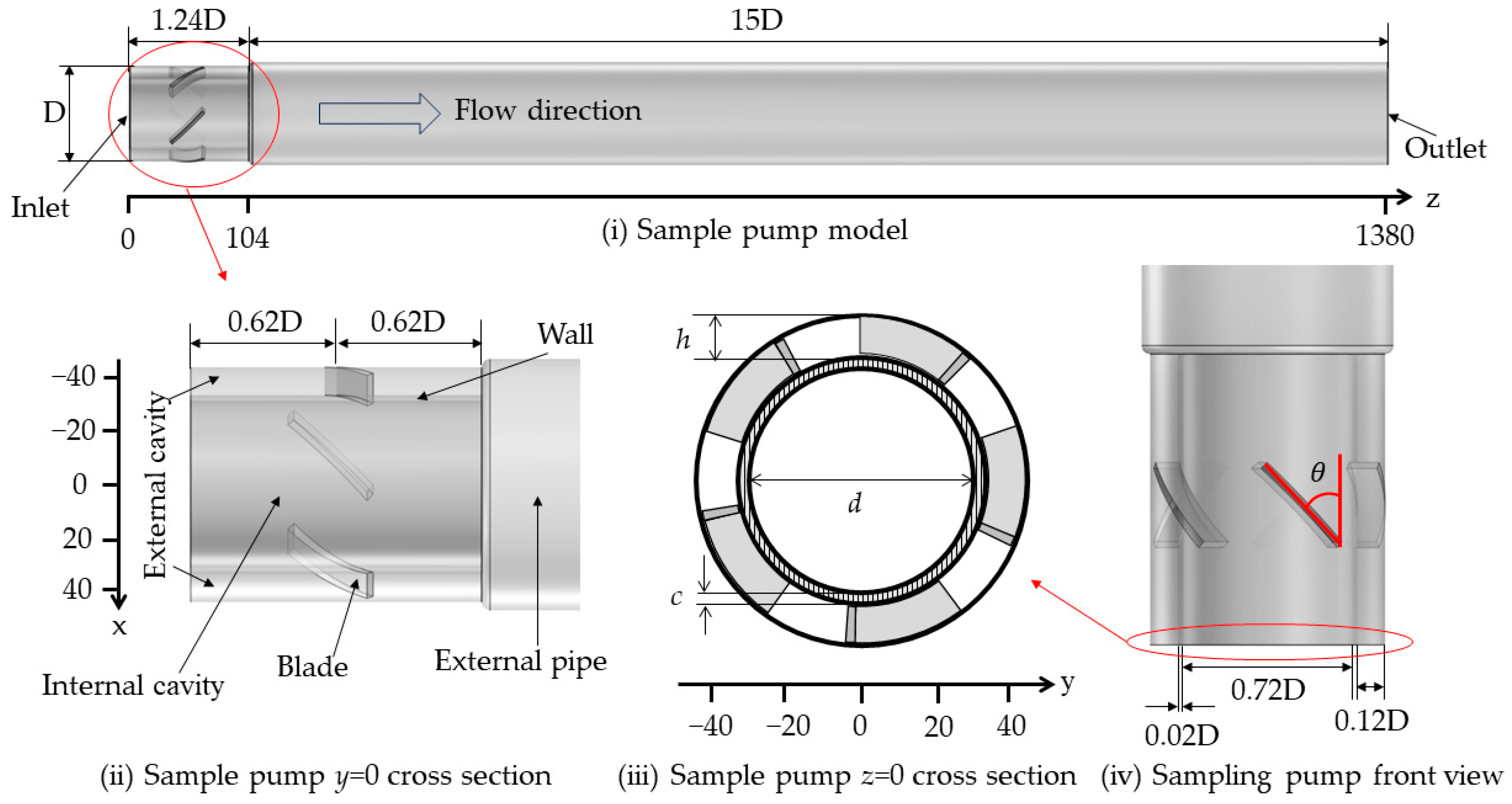
3.2. Geometric Models and Boundary Conditions

The numerical model of the sampling pump is shown in Figure 2. The inlet diameter of the model is D = 84 mm, in which the diameter of the internal cavity is 0.72D, the wall thickness of the internal and external cavity is 0.02D, and the cross-section scale of the external cavity is 0.12D. The sampling pump body is 1.24D, and the external pipe is 15D. To ensure that the flow in the external pipe is fully developed, the blade angle is 45°, and the number of the blades is five. In the simulation, the fluid is set as water, the temperature is 293.15 K, the density is 1000 kg/m³, and the dynamic viscosity is 9 × 10⁻⁴ Pa·s. The external cavity blade of the model is set as the rotating region and the rest as the static region by using the multi-reference freezing rotor method. The boundary conditions of the entrance and exit are pressure, and the gauge pressure is 0 Pa. The inner wall adopts a standard wall function, and the velocity boundary conditions on the wall are non-slip wall conditions [29,30,31].

3.3. Grid Independence Test

To ensure the calculation is accurate, firstly, the influence of the mesh partition on the calculation results is analyzed. The grid is a tetrahedral structure, with four nodes in each grid. The main basis for grid division is to refine the blade part, and the boundary layers with four different numbers of grids are 3, 4, 5, and 6, respectively. Four groups of different grid elements were divided and calculated with a blade rotational speed of n = 270 rpm. The time step was 0.1 s, and 16 iterations were performed in each step. Equation residual less than 1 × 10⁻³ is used as the convergence criterion. The results of four models with different cell mesh numbers were analyzed, and the flow rate at the internal cavity inlet of the sampling pump Q is shown in

Table 1. Flow rate at the internal cavity inlet for different grid numbers.

Group	Number of Grid	Q
Grip 1	106,548	2.71 m3/h
Grip 2	140,609	3.22 m3/h
Grip 3	180,542	3.50 m3/h
Grip 4	221,084	3.50 m3/h

. When the number of grids is higher than 180,542, the flow rate does not change; too few grids will lead to increased errors. With the increase in the number of grids, the calculation accuracy increases, but the calculation time and computation cost also increase [32]. After comprehensive consideration, the grid number is selected at 180,542, as shown in Figure 3. At this time, the y+ value of the wall is 31~200 [33].

3.4. Time Independent Analysis

The time-independent analysis of the numerical simulation results was further carried out. The area-weighted velocities at the internal cavity inlet (ICI) and outlet of the pipe, and the pressure at the internal cavity outlet (ICO) varying with time, have been presented in Figure 4. The simulation time runs up to 30 s. Before 7 s, the area-weighted velocity and pressure increase sharply with time. After 10 s, both the velocity and pressure tended to be stable. The following time average analysis averages results between 10–30 s, and the colored contours take instantaneous results at 15 s.

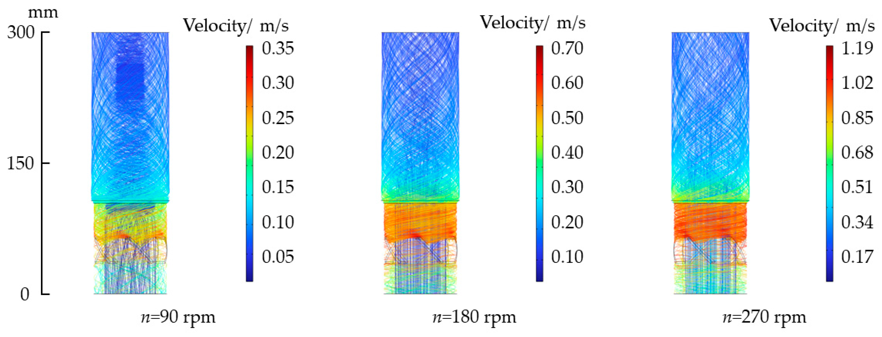
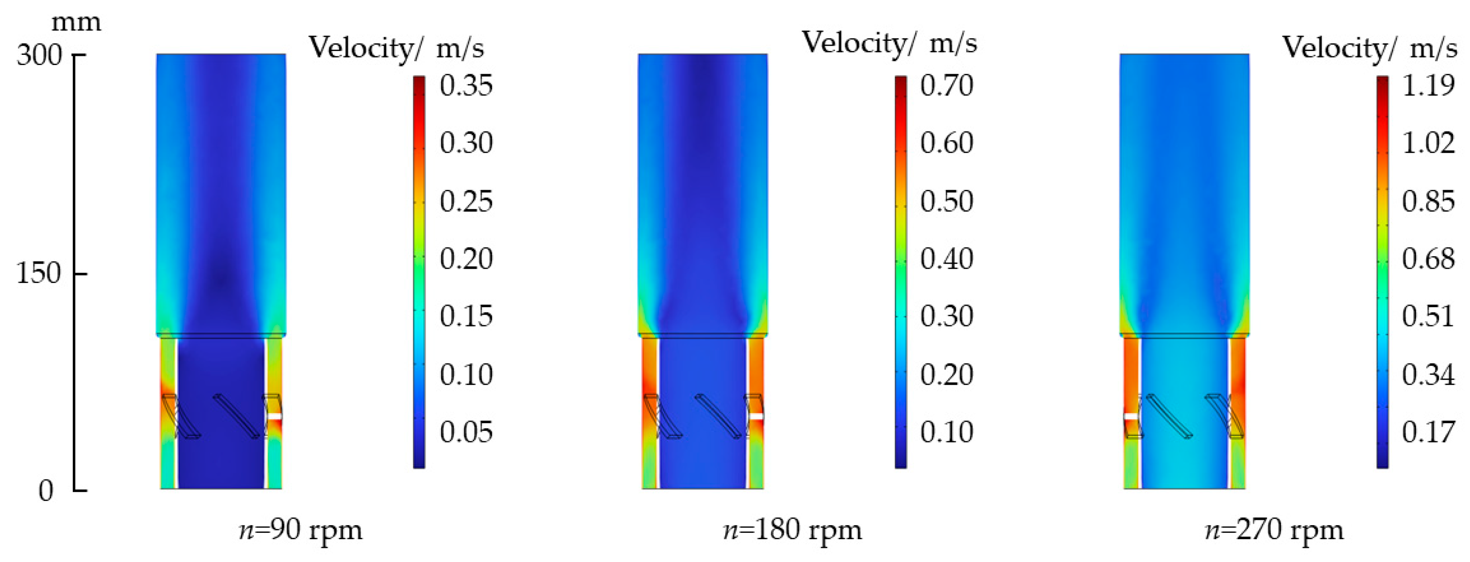
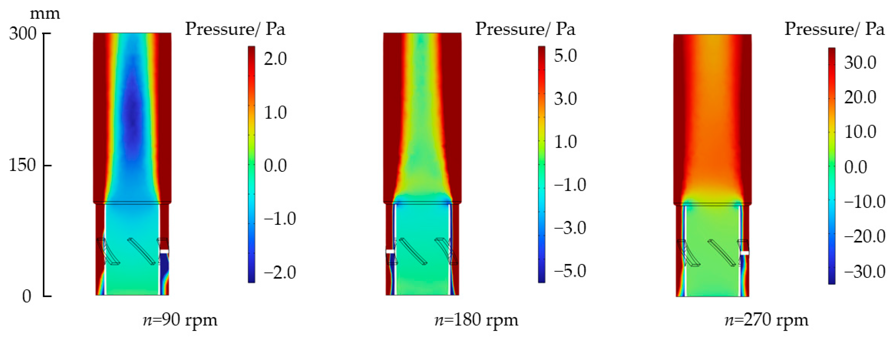
4. Effects of Rotational Speed on the Flow Rate

Rotational speed is an important parameter in the sampling process, which determines the feasibility of sampling and the flow rate. In the numerical simulation, three different rotational speeds at n = 90, 180, and 270 rpm were simulated in this paper, and the rotor was increased to the corresponding speed in 0.1 s by the step function. The results show that the velocity does not change significantly around the 11D length of the external pipe after the flow field is stable. In order to better present the results, a part of the inlet to flow direction with a length of 300 mm is selected for analysis. The transient streamlines from the inlet and colored contours of velocity, pressure, and turbulent kinetic energy at 15 s on the plane y = 0 are shown in Figure 5, Figure 6, Figure 7 and Figure 8.

It can be seen from the streamlines in Figure 5, driven by the rotor blade, the water flow in the external cavity moves forward in a spiral manner, and the water flow in the central part of the external pipe also moves forward in a spiral manner with the water flow in the external cavity.

In the colored contours of velocity shown in Figure 6, high-speed water flows toward the external pipe. When the rotational speed of the external cavity blade increases, the water velocity in the external cavity also increases correspondingly, and the velocity of the water in the internal cavity also increases. The highest point of the velocity is located at the front of the external cavity blade, while the lowest point of the velocity appears in different positions under different rotational speeds. Due to the increase in viscous force and cross-section of the pipe, the velocity of the fluid in the external cavity decreases after entering the pipe.

In the rotor section in Figure 7, centrifugal force causes the pressure to increase outward in a radial direction [34,35]. A pressure difference is formed between the inside and outside at the outlet of the internal cavity. Furthermore, the pressure at the outlet of the internal cavity is less than that at the internal cavity inlet. As a result, a negative pressure forms between the outlet and inlet of the internal cavity, and the seawater in the sampling pump internal cavity flows from the inlet to the outlet under the action of the positive pressure gradient. In Figure 8, it can be seen that the turbulent kinetic energy is larger in the external cavity, external cavity outlet, and the zone near the wall of the external pipe, while the turbulent kinetic energy in the internal cavity is smaller and becomes more pronounced with the increase in rotational speed. This also reflects that the energy is mainly concentrated in the external cavity and its outlet. A smaller turbulent kinetic energy in the internal cavity can make planktonic organisms pass through more smoothly. The pumping effect is different at different rotational speeds, and the higher the rotor rotational speed, the larger the inlet flow of the sampling pump. The results of area-weighted and time average velocity at the external cavity inlet ${〈\overline{V}〉}_{ECI}$ and the internal cavity inlet ${〈\overline{V}〉}_{ICI}$, as well as the flow rate Q at the internal cavity inlet with different rotational speeds, are shown in

Table 2. Time and area-weighted average velocity and flow rate at different n.

n	${〈\overline{\mathit{V}}〉}_{\mathit{E}\mathit{C}\mathit{I}}$	${〈\overline{\mathit{V}}〉}_{\mathit{I}\mathit{C}\mathit{I}}$	F
90 rpm	0.25 m/s	0.03 m/s	0.30 m3/h
180 rpm	0.51 m/s	0.13 m/s	1.30 m3/h
270 rpm	0.84 m/s	0.35 m/s	3.50 m3/h

. When the rotational speed n increases from 90 rpm to 270 rpm, the flow rate at the internal cavity inlet increases from 0.3 m³/h to 3.5 m³/h. When the rotational speed n is 180 rpm, the flow rate is 1.3 m³/h, which is slightly higher than the design requirement.

Figure 9i shows the velocity and pressure distribution along the streamwise direction in the external cavity at 15 s. The external cavity blade works on the water and generates mechanical energy, which makes the fluid velocity increase sharply. After entering the external pipe, the velocity of the fluid decreases and becomes stable at about 800 mm (9.52D). The pressure fluctuates at blades because of the difference in pressure between the front and back of the blade during rotation, and the pressure drops to 0 at the outlet of the model. Figure 9ii shows the velocity and pressure distribution along the streamwise direction in the internal cavity. The velocity on the central axis decreases slightly along the flow direction in the internal cavity and then decreases rapidly after a slight local rise near the outlet of the internal cavity. The velocity drops to the lowest point at z = 350 mm and then increases slowly. After z = 998 mm, the velocity basically does not change. From the inlet to the outlet of the internal cavity, the pressure at z = 182 mm dropped sharply to the lowest point, which is also the reason for the pump’s automatic suction, then the overall pressure gradually increased, and the pressure at z = 711 mm rose to the highest point, and the pressure began to decline slowly along the flow direction at the pipe outlet.

Numerical simulation results show that the negative pressure near the outlet of the internal cavity is the reason for the realization of the automatic suction pump [36,37]. Through numerical simulation, the relationship between different blade rotational speeds and internal cavity inlet flow rates is obtained. The internal cavity flow rate is highly correlated with the blade rotational speed. The faster the rotational speed, the higher the flow rate in the internal cavity.

5. Effects of Structural Parameters on the Flow Rate at the Internal Cavity Inlet

The influence of structural parameters on the internal cavity inlet flow rate under a fixed rotational speed has been numerically studied further. The effects of internal and external cavity size (external cavity width h = 10, 12, 14, 16 mm), blade angle (θ = 30°, 40°, 45°, 50°, 60°), and number of blades (s = 3, 4, 5, 6) on the inlet flow rate of the internal cavity of the shaftless hollow sampling pump model were numerically simulated to obtain the maximum flow at a fixed rotational speed. The number of grids corresponding to each structural size is different, but all examples use the grid independence test in Section 3.3 to keep the boundary with five layers and the number of grids around 180,000.

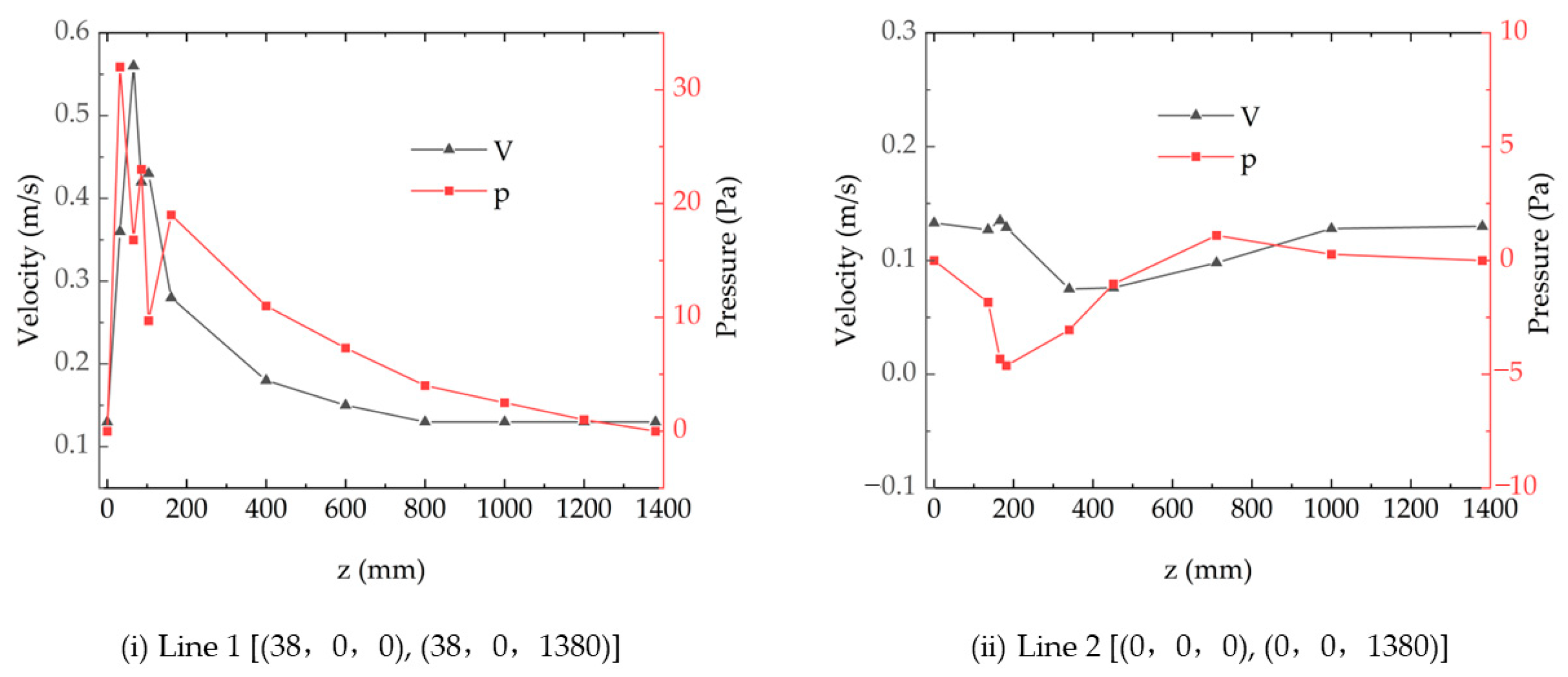
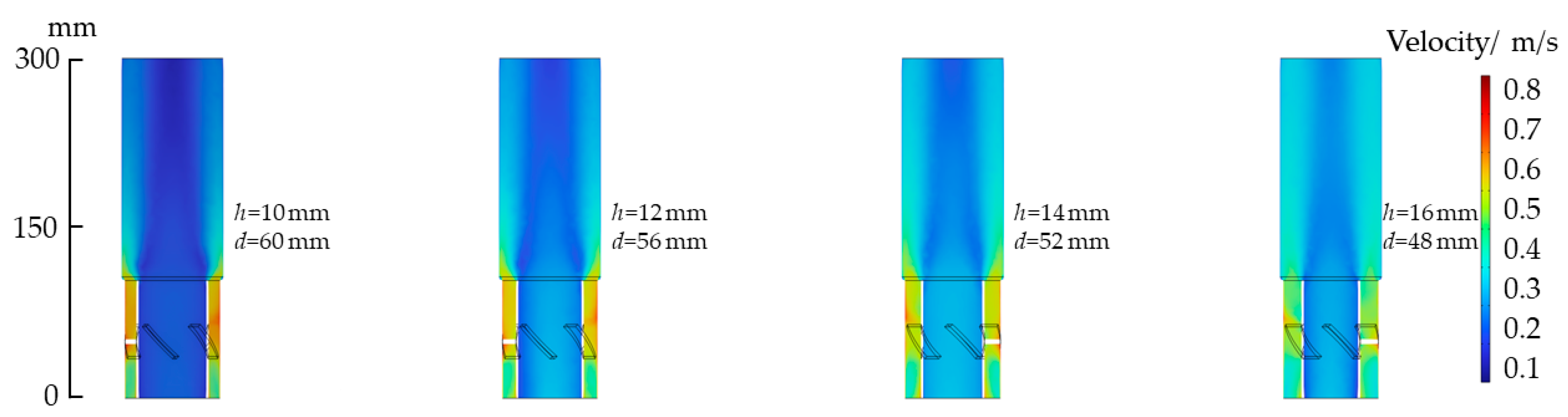
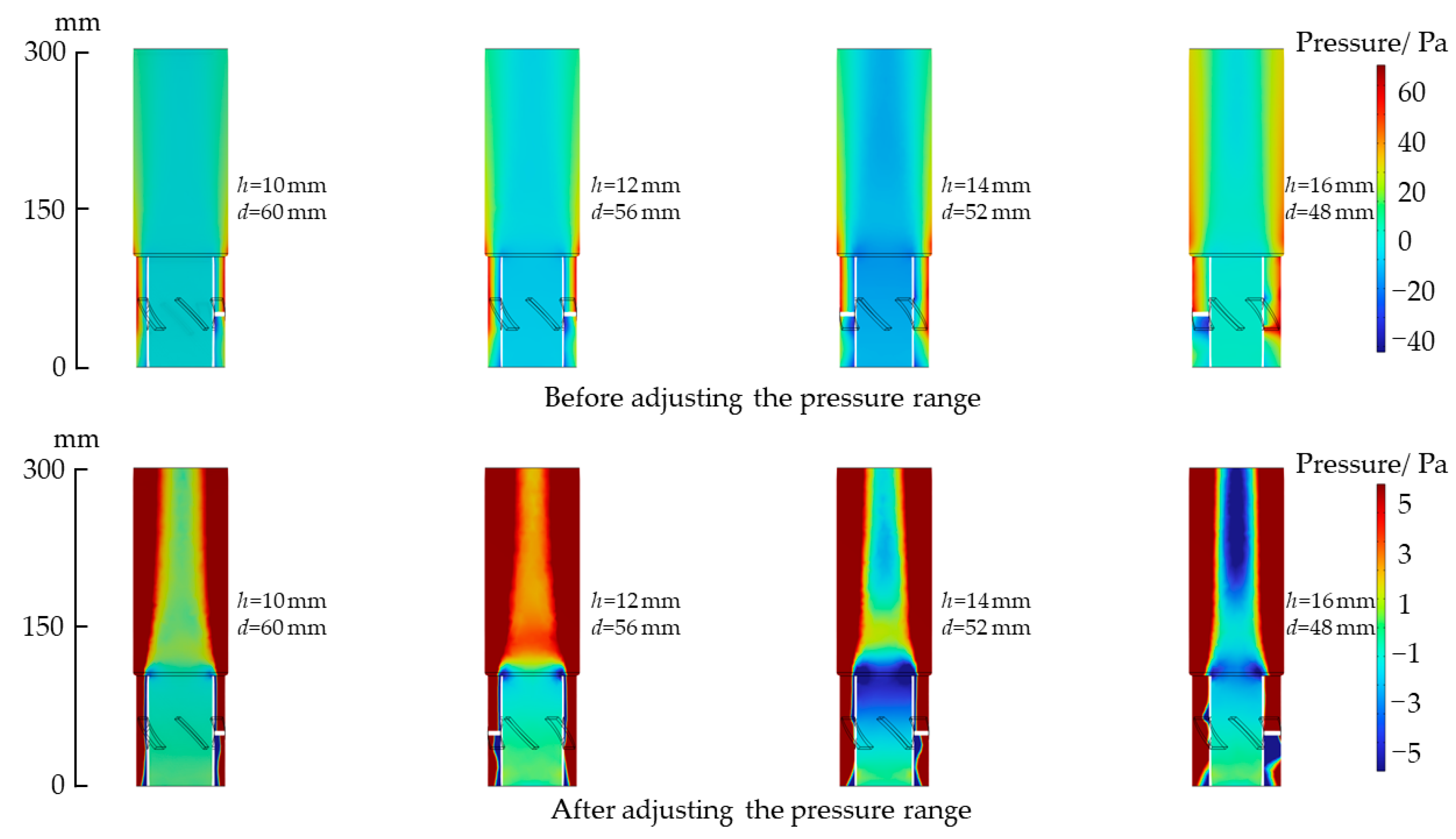
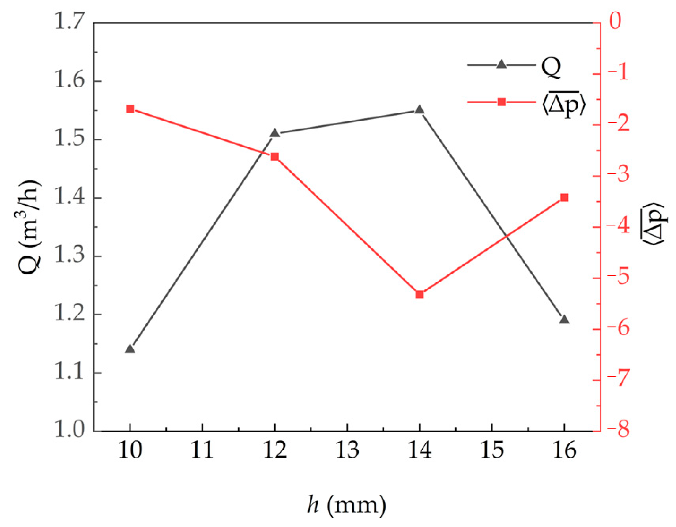
5.1. Effects of Internal and External Cavity Size on the Inlet Flow Rate

The dimensions and structural parameters of different internal and external cavities are shown in Figure 2iii and

Table 3. Dimensions of internal and external cavities.

Group	h (mm)	d (mm)	c (mm)
Size 1	10	60	2
Size 2	12	56	2
Size 3	14	52	2
Size 4	16	48	2

. The wall thickness keeps c = 2 mm, the width of the external cavity h increases, and the diameter of the internal cavity d decreases, while d + 2c + 2h = D remains unchanged.

The rotational speed keeps constant, n = 180 rpm. The colored contours of the pressure and velocity on the y = 0 at 15 s is shown in Figure 10 and Figure 11.

At the same rotational speed, Figure 10 shows that the velocity in the internal cavity doesn’t show a linear relationship with the increase of h, but increases first and then decreases, and the maximum velocity is obtained when h is minimum in the external cavity. In order to make the pressure of the internal cavity more obvious, we adjust the pressure range in Figure 11. It can be seen that the pressure difference between the inlet and outlet of the internal cavity is the largest when h = 14 after adjusting the legend. At the same cross-section position, the pressure of the external cavity is greater than that of the internal cavity. Figure 12 shows the four groups of time average flow rate and $〈\overline{∆p}〉$. It is defined that $〈\overline{∆p}〉$ = ${〈\overline{p}〉}_{ICO}$ − ${〈\overline{p}〉}_{ICI}$, where ${〈\overline{p}〉}_{ICO}$ and ${〈\overline{p}〉}_{ICI}$ are the area-weighed and time average pressure at the internal cavity outlet and the internal cavity inlet respectively, as shown in Figure 1. It should be noted that here ${〈\overline{p}〉}_{ICI}=0.$ The average time ranges from 10 to 30 s. When h = 14 mm, the flow rate is the highest, and the negative pressure difference is the largest, which is 1.55 m³/h and −5.3 Pa, respectively. When h = 10 mm, the flow rate is the lowest, and the negative pressure difference is the smallest, which are 1.14 m³/h and −1.68 Pa, respectively. According to equation (10), the flow rate relative difference $r$ for different internal and external cavity sizes is 35.96%. Under the fixed cross-section size and wall thickness, the internal and external cavity sizes have a significant influence on the flow rate at the internal cavity inlet. When the external cavity has h = 14 mm, and the internal cavity diameter is d = 52 mm, the flow rate at the internal cavity inlet is the largest, and the effect is the best.

$$r=\frac{Q_{max}-Q_{min}}{Q_{min}}\times 100\mathrm{\%}$$

(10)

where $r$ is the relative difference of the flow rate, $Q_{max}$ is the maximum flow rate, and $Q_{min}$ is the minimum flow rate.

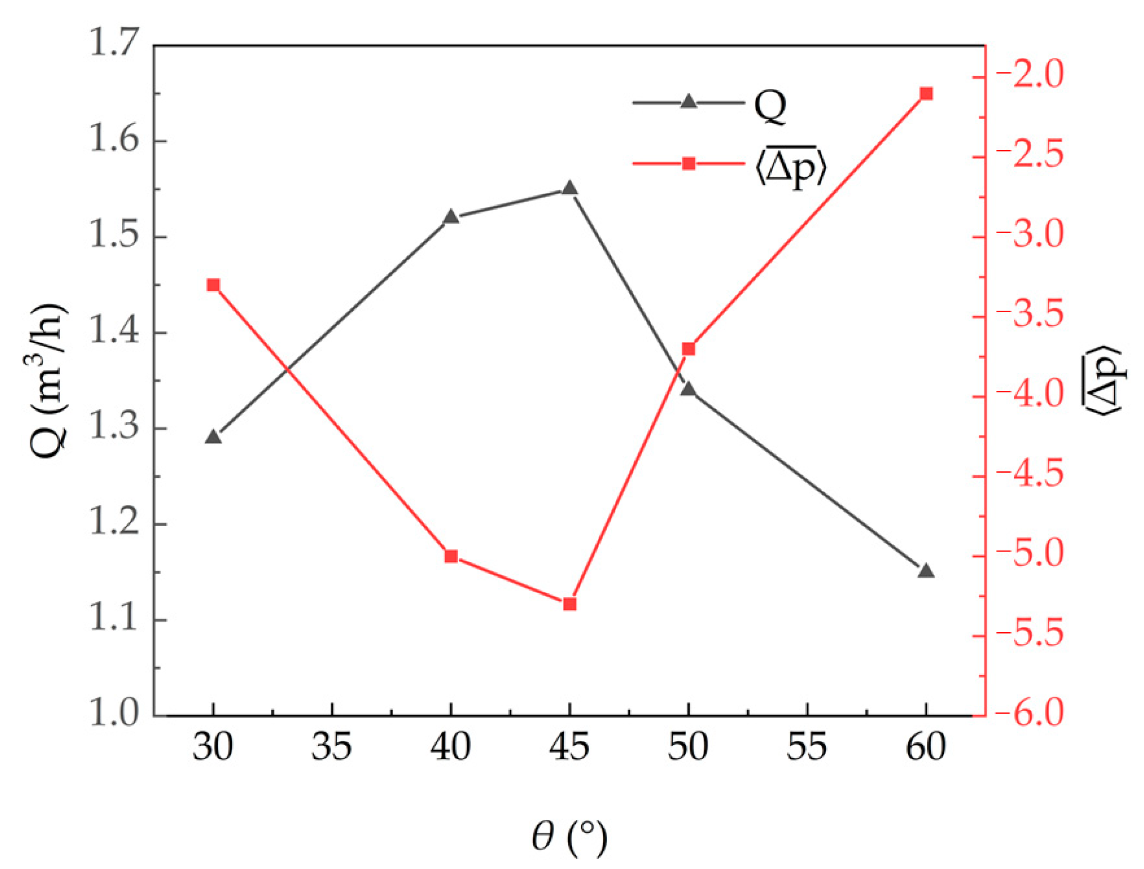
5.2. Effects of Blade Angle on the Flow Rate at the Internal Cavity Inlet

We take h = 14 mm, d = 52 mm, and n = 180 rpm and perform numerical simulation on blade angles θ = 30°, 40°, 45°, 50°, and 60°, respectively, to study the effect of blade angle on the flow rate at the internal cavity inlet.

As shown in Figure 13, the structural parameters that obtained the maximum flow rate at the internal cavity inlet are not in the case of blade angles that are too large or too small [38,39]. The pump suction rate increases with the blade angle from 30° to 45° and decreases from 45° to 60°. When the blade angle is 45°, the pressure difference and the flow rate are the largest, which are −5.3 Pa and 1.55 m³/h, respectively. When the blade angle is 60°, the pressure difference and the flow rate are the smallest, which are −2.1 Pa and 1.15 m³/h, respectively. According to Equation (10), the maximum relative difference of the flow rate between different blade angles is 34.78%. At the same rotating speed, the blade angle has a significant effect on the flow rate of the internal cavity, and the maximum flow rate reaches 45°.

5.3. Effects of Blade Numbers on the Flow Rate at the Internal Cavity Inlet

We take h = 14 mm, d = 52 mm, and n = 180 rpm and perform numerical simulation on the number of blades (s = 3, 4, 5, 6, respectively). The Q and $〈\overline{∆p}〉$ at the internal cavity inlet are shown in Figure 14, and the number of blades does not affect the flow rate at the internal cavity inlet significantly compared with the former two structural parameters. The flow rate increases at three to five blades and then decreases. The minimum flow rate (s = 3) and the maximum flow rate (s = 5) are 1.44 m³/h and 1.55 m³/h, respectively, and the difference is only 0.11 m³/h. The pressure difference between the inlet and outlet of the internal cavity is −4.5 Pa and −5.3 Pa, respectively. According to Equation (10), the relative flow rate difference for different blade numbers is 7.63%. When n = 180 rpm, the number of blades has a relatively lesser effect on the inlet flow rate, and the flow rate of the internal cavity inlet reaches a maximum with five blades.

6. Instrument Design and Experiment Verification

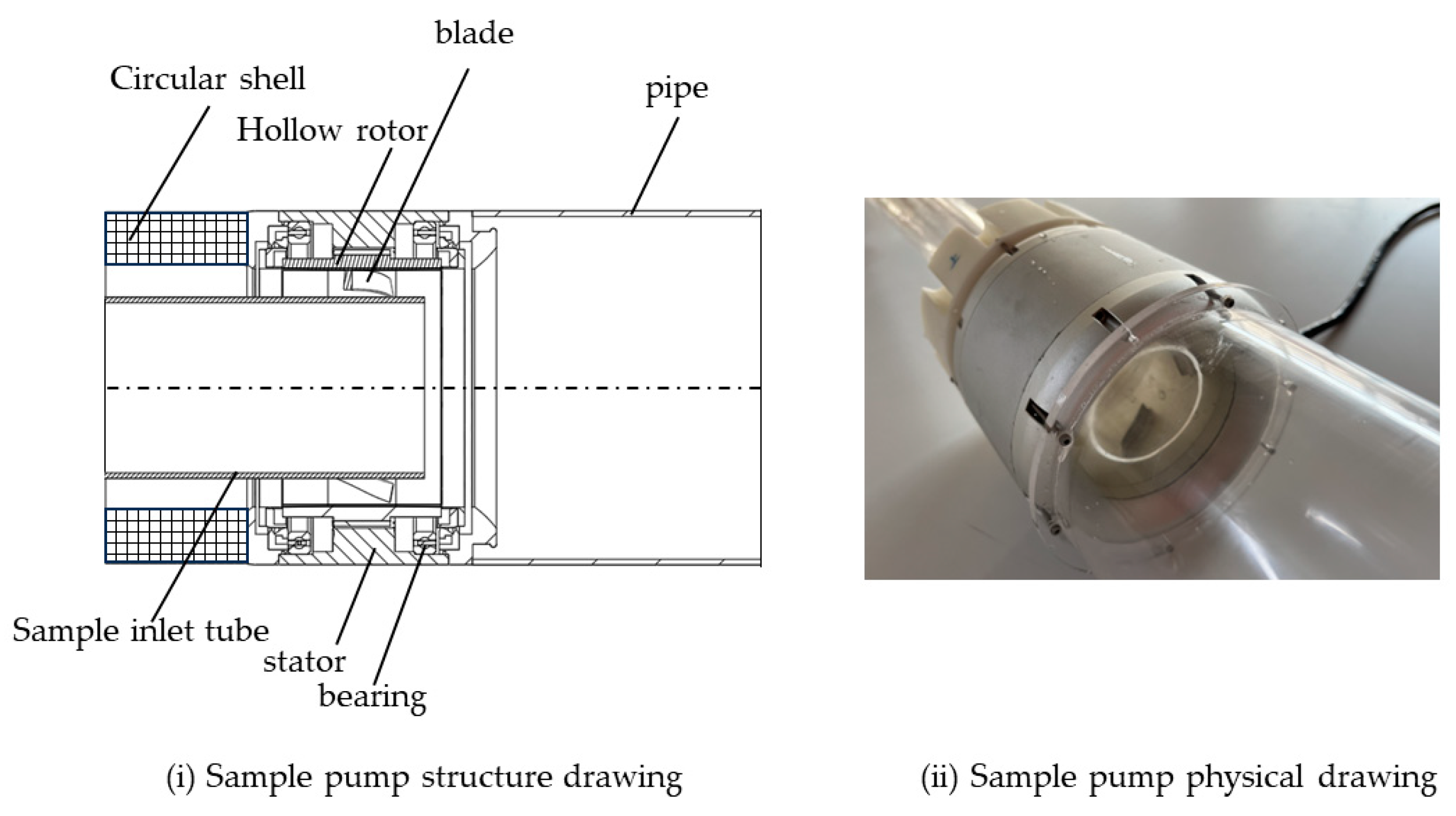
6.1. Shaftless Hollow Pump Design

Based on the results of the above analysis, a shaftless hollow pump is designed and produced. The structure diagram and the instrument are shown in Figure 15. The pump consists of a DC brushless motor, blades, sample inlet tube, pipe, and other components. The rated voltage of a brushless DC motor is 24 V. The stator is fixed to the circular shell through the end cover, and the sealing ring is added to the end cover to waterproof and withstand pressure. The inner diameter of the hollow rotor is 84 mm, and it is installed inside the stator. The blades are mounted on a hollow rotor. Angular contact bearings are used to bear the load during the high-speed impeller flow. The circular shell is also fixed to the sample inlet tube; the inner diameter of the sample inlet tube is 52 mm. The annular space between the rotor and the sample inlet tube is a high-speed flow cavity with a spacing of 14 mm. The five blades are arranged in the high-speed thrust cavity inside the rotor at an angle of 45°.

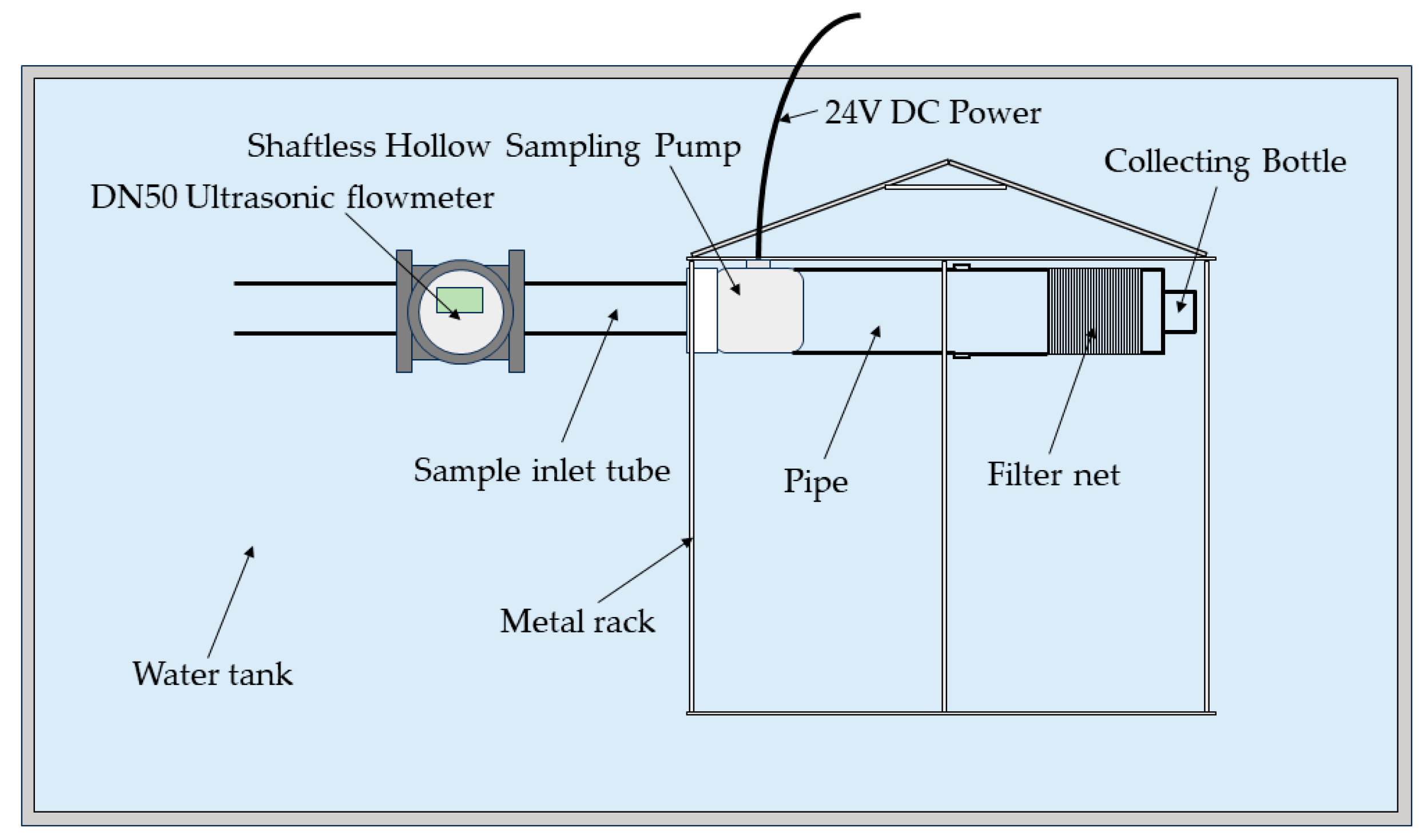
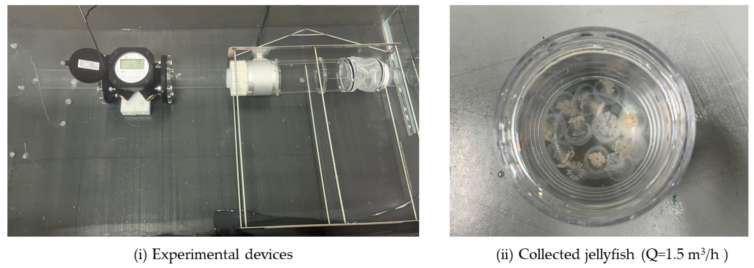
6.2. Experiment Verification

To verify the feasibility and non-damage of the sampling pump, the experimental setup shown in Figure 16 was designed. A DN50 ultrasonic flowmeter is installed on the sample inlet tube at the front of the pump to monitor the suction water flow with an accuracy of 0.01 m³/h. A filter screen and a collection bottle are installed at the end of the pipe to collect plankton samples. The whole device was placed in a water tank, in which 12 jellyfish (Rhopilema esculentum Kishinouye) with a size of 1–2 cm were placed for the collection experiment. A 24V DC power supply is used to regulate the current to control the motor speed. The actual scene of the experimental device is shown in Figure 17i.

By adjusting the motor rotational speed, 1.50 m³/h pump suction flow was sampled, and the time was set to 10 min. The jellyfish were collected in the experiment, as shown in Figure 17ii, and the jellyfish remained intact without being damaged, which proved the feasibility of the pump suction sample proposed in this paper.

7. Conclusions

In this paper, a new sampling method based on a shaftless hollow sampling pump is proposed. The designed sampling pump can be used as the driving part of the plankton filter sampler. It is a new sampling method for plankton.

The numerical model of a shaftless hollow pump is established, and the suction flow of the pump at different rotational speeds is studied using the computational fluid dynamics method. We analyzed the velocity and pressure in the internal and external cavities of the hollow sampling pump and the external pipe and elucidated the principle of non-destructive sampling in the hollow sampling pump. The effects of the width of the internal and external cavities, blade angle, and number of blades on the flow rate of the internal cavity inlet at a certain rotational speed and the total size of the cross-section are further studied. The results show that the higher the blade rotational speed, the greater the inlet flow. At a fixed rotational speed, the internal and external cavity size and blade angle have significant effects on the flow rate of the internal cavity inlet, while the number of blades has relatively little influence on the inlet flow. Taking n = 180 rpm as an example, when the internal and external cavities are h = 14 mm and d = 52 mm, the blade angle is 45°, and the number of blades is five, the flow rate at the internal cavity inlet of the sampling pump is the highest. All cases show that the flow rate at the internal cavity inlet is directly related to the negative pressure difference between the internal cavity outlet and inlet. The greater the negative pressure at the internal cavity outlet, the greater the flow rate at the internal cavity inlet.

Finally, the sampling pump is designed and manufactured, and the laboratory pool experiment is designed to carry out jellyfish sampling. The experimental results show that the suction flow of the shaftless hollow pump can reach more than 1.50 m³/h, and the non-destructive capture of jellyfish can be realized.

The shaftless hollow pump designed in this paper can provide the key core components of the fixed-point filter sampler for plankton in the ocean so as to realize efficient, non-destructive sampling of fixed-point flow, which is of great significance for the study of marine plankton.

References

1. Drits, A.V.; Pasternak, A.F.; Kravchishina, M.D. The Role of Plankton in the Vertical Flux in the East Siberian Sea Shelf. Oceanology 2019, 59, 669–677. [Google Scholar] [CrossRef]
2. Gruber, A.; Medlin, L.K. Complex Plastids and the Evolution of the Marine Phytoplankton. J. Mar. Sci. Eng. 2023, 11, 1903. [Google Scholar] [CrossRef]
3. Ostle, C.; Paxman, K.; Graves, C.A. The Plankton Lifeform Extraction Tool: A digital tool to increase the discoverability and usability of plankton time-series data. Earth Syst. Sci. Data 2021, 13, 5617–5642. [Google Scholar] [CrossRef]
4. Nishikawa, J.; Tsuda, A. Diel vertical migration of the tunicate Salpa thompsoni in the Southern Ocean during summer. Polar Biol. 2001, 24, 299–302. [Google Scholar] [CrossRef]
5. Weibo, P.H.; Morton, A.W.; Bradley, A.M. New development in the MOCNESS, an apparatus for sampling zooplankton and micronekton. Mar. Biol. 1985, 87, 313–323. [Google Scholar]
6. Weibo, P.H.; Burt, K.H.; Boyd, S.H. A multiple opening closing net and environmental sensing system for sampling zoo plankton. J. Mar. Res. 1976, 34, 313–326. [Google Scholar]
7. Strand, E.; Broms, C.; Bagoien, E. Comparison of two multiple plankton samplers: MOCNESS and Multinet Mammoth. Limnol. Oceanogr. Methods 2022, 20, 595–604. [Google Scholar] [CrossRef]
8. Kilburn, R.; Bricknell, I.R.; Cook, P. Design and application of a portable, automated plankton sampler for the capture of the parasitic copepods Lepeophtheirus salmonis (Kr circle divide yer 1837) and Caligus elongatus (Von Nordmann 1832). J. Plankton Res. 2010, 32, 967–970. [Google Scholar] [CrossRef]
9. Guillam, M.; Bessin, C. Vertical distribution of brittle star larvae in two contrasting coastal embayments: Implications for larval transport. Sci. Rep. 2020, 10, 12033. [Google Scholar] [CrossRef]
10. Weidberg, N.; Goschen, W.; Jackson, J.M. Fine scale depth regulation of invertebrate larvae around coastal fronts. Limnol. Oceanogr. 2019, 64, 785–802. [Google Scholar] [CrossRef]
11. Wilborn, R.E.; Rooper, C.N.; Goddard, P. A novel design for sampling benthic zooplankton communities in disparate Gulf of Alaska habitats using an autonomous deep-water plankton pump. J. Plankton Res. 2020, 42, 457–466. [Google Scholar] [CrossRef]
12. Billings, A.; Kaiser, C.; Young, C.M. SyPRID sampler: A large-volume, high-resolution, autonomous, deep-ocean precision plankton sampling system. Deep. Sea Res. Part II-Top. Stud. Oceanogr. 2017, 137, 297–306. [Google Scholar] [CrossRef]
13. Zhou, L.; Bai, L.; Li, W.; Shi, W.; Wang, C. PIV validation of different turbulence models used for numerical simulation of a centrifugal pump diffuser. Eng. Comput. 2018, 35, 2–17. [Google Scholar] [CrossRef]
14. Zhou, L.; Hang, J.; Bai, L.; Krzemianowski, Z.; El-Emam, M.A.; Yasser, E.; Agarwal, R. Application of entropy production theory for energy losses and other investigation in pumps and turbines: A review. Appl. Energy 2022, 318, 119211. [Google Scholar] [CrossRef]
15. Fracassi, A.; De Donno, R.; Ghidoni, A.; Noventa, G. Assessment of an Improved Delayed X-LES Hybrid Model for the Study of Off-Design Conditions in Centrifugal Pumps. J. Fluids Eng. 2022, 144, 101501. [Google Scholar] [CrossRef]
16. El-Emam, M.; Zhou, L.; Yasser, E.; Bai, L.; Shi, W. Computational methods of erosion wear in centrifugal pump: A state-of-the-art review. Arch. Comput. Methods Eng. 2022, 29, 3789–3814. [Google Scholar] [CrossRef]
17. Shih, T.H.; Liou, W.W.; Shabbir, A.; Yang, Z.; Zhu, J. A New k-ε Eddy-Viscosity Model for High Reynolds Number Turbulent Flows—Model Development and Validation. Comput. Fluids 1995, 24, 227–238. [Google Scholar] [CrossRef]
18. Launder, B.E.; Spalding, D.B. Lectures in Mathematical Models of Turbulence; Academic Press: Cambridge, MA, USA, 1972. [Google Scholar]
19. Orszag, S.A.; Yakhot, V.; Flannery, W.S.; Boysan, F.; Choudhury, D.; Maruzewski, J.; Patel, B. Renormalization Group Modeling and Turbulence Simulations. In Proceedings of the International Conference on Near-Wall Turbulent Flows, Tempe, AZ, USA, 15–17 March 1993. [Google Scholar]
20. Wilcox, D.C. Turbulence Modeling for CFD; DCW Industries: La Canada, CA, USA, 1998. [Google Scholar]
21. Menter, F.R. Two-Equation Eddy-Viscosity Turbulence Models for Engineering Applications. AIAA J. 1994, 32, 1598–1605. [Google Scholar] [CrossRef]
22. De Donno, R.; Fracassi, A.; Ghidoni, A.; Morelli, A.; Noventa, G. Surrogate-Based Optimization of a Centrifugal Pump with Volute Casing for an Automotive Engine Cooling System. Appl. Sci. 2021, 11, 11470. [Google Scholar] [CrossRef]
23. De Donno, R.; Fracassi, A.; Noventa, G.; Ghidoni, A.; Bebay, S. Surrogate-based shape optimization of centrifugal pumps for automotive engine cooling systems. In Advances in Evolutionary and Deterministic Methods for Design, Optimization and Control in Engineering and Sciences; Springer: Cham, Switzerland, 2021; pp. 277–290. [Google Scholar]
24. Guo, R.; Li, R.; Zhang, R.; Han, W. Numerical Study of the Unsteady Flow Characteristics of a Jet Centrifugal Pump under Multiple Conditions. Processes 2019, 7, 786. [Google Scholar] [CrossRef]
25. Wang, C.S.; Zhang, L. Fluid simulation in a cyclone reverse circulation well washing device based on computational fluid dynamics. Energy Sci. Eng. 2019, 7, 1306–1314. [Google Scholar] [CrossRef]
26. Agrawal, K.K.; Bhardwaj, M.; Misra, R.; Das Agrawal, G.; Bansal, V. Optimization of operating parameters of earth air tunnel heat exchanger for space cooling: Taguchi method approach. Geotherm. Energy 2018, 6, 10. [Google Scholar] [CrossRef]
27. Tian, W.; Song, B.; Mao, Z. Conceptual design and numerical simulations of a vertical axis water turbine used for underwater mooring platforms. Int. J. Nav. Archit. Ocean. Eng. 2013, 5, 625–634. [Google Scholar]
28. Li, R.; Gong, J.; Chen, W.; Li, J.; Chai, W.; Rheem, C.k.; Li, X. Numerical Investigation of Vortex-Induced Vibrations of a Rotating Cylinder near a Plane Wall. J. Mar. Sci. Eng. 2023, 11, 1202. [Google Scholar] [CrossRef]
29. Chen, C.; Song, Y.L.; Xie, Y.D. Simulation and analysis of inclined flow channel of hydraulic slide valve. J. Phys. Conf. Ser. 2020, 1707, 012011. [Google Scholar] [CrossRef]
30. Lin, Z.; Yang, F.; Guo, J.; Jian, H.; Sun, S.; Jin, X. Leakage Flow Characteristics in Blade Tip of Shaft Tubular Pump. J. Mar. Sci. Eng. 2023, 11, 1139. [Google Scholar] [CrossRef]
31. Jiao, H.; Wang, M.; Liu, H.; Chen, S. Positive and Negative Performance Analysis of the Bi-Directional Full-Flow Pump with an “S” Shaped Airfoil. J. Mar. Sci. Eng. 2023, 11, 1188. [Google Scholar] [CrossRef]
32. Feng, H.; Wan, Y.; Fan, Z. Numerical investigation of turbulent cavitating flow in an axial flow pump using a new transport-based model. J. Mech. Sci. Technol. 2020, 34, 745–756. [Google Scholar] [CrossRef]
33. Zhu, D.; Yan, W.; Guang, W.; Wang, Z.; Tao, R. Influence of Guide Vane Opening on the Runaway Stability of a Pump-Turbine Used for Hydropower and Ocean Power. J. Mar. Sci. Eng. 2023, 11, 1218. [Google Scholar] [CrossRef]
34. Yang, F.; Li, Z.; Hu, W.; Liu, C.; Jiang, D.; Liu, D.; Nasr, A. Analysis of flow loss characteristics of slanted axial-flow pump device based on entropy production theory. R. Soc. Open Sci. 2022, 9, 211208. [Google Scholar] [CrossRef]
35. Cui, B.; Han, X.; An, Y. Numerical Simulation of Unsteady Cavitation Flow in a Low-Specific-Speed Centrifugal Pump with an Inducer. J. Mar. Sci. Eng. 2022, 10, 630. [Google Scholar] [CrossRef]
36. Duan, X.D.; Sun, X.Q. The Experimental Study on Compositional Parameters of the Annular Multinozzle Jet Pump. Prospect. Eng. 1999, 6, 17–19. [Google Scholar]
37. Yuan, D.Q.; Wang, G.J.; Wu, J. Numerical simulation and experiment study on multi-nozzle jet pump. Trans. Agric. Eng. 2008, 24, 95–99. [Google Scholar]
38. Yang, C.; Zhang, Q.; Guo, J.; Wu, J.; Zheng, Y.; Ren, Z. Optimal Design and Fish-Passing Performance Analysis of a Fish-Friendly Axial Flow Pump. Appl. Sci. 2023, 13, 12056. [Google Scholar] [CrossRef]
39. Zhu, Z.; Liu, H. Experimental Research and Numerical Analysis of Pressure Fluctuation Characteristics of Rim Driven Propulsion Pump Outlet. Machines 2021, 9, 293. [Google Scholar] [CrossRef]
Figure 1. Principle diagram of a shaftless hollow sampling pump.
Jmse 12 00284 g001
Figure 2. Geometric model of sampling pump.
Jmse 12 00284 g002
Figure 3. Mesh of the sampling pump model.
Jmse 12 00284 g003
Figure 4. Area-weighted velocities (i) and pressure (ii) varying with time.
Jmse 12 00284 g004
Figure 5. Streamlines from the inlet with different n.
Jmse 12 00284 g005
Figure 6. Colored contours of velocity with different n on the plane y = 0.
Jmse 12 00284 g006
Figure 7. Colored contours of pressure with different n on the plane y = 0.
Jmse 12 00284 g007
Figure 8. Colored contours of turbulent kinetic energy with different n on the plane y = 0.
Jmse 12 00284 g008
Figure 9. Instantaneous velocity and pressure distributions along the streamwise direction in the external (i) and internal (ii) cavities.
Jmse 12 00284 g009
Figure 10. Colored contours of velocity for different internal and external cavity size on the plane y = 0.
Jmse 12 00284 g010
Figure 11. Colored contours of pressure for different internal and external cavity size on the plane y = 0.
Jmse 12 00284 g011
Figure 12. The flow rate at the internal cavity inlet and p ¯ with different internal and external cavities size.
Jmse 12 00284 g012
Figure 13. The flow rate at the internal cavity inlet and p ¯ of sampling pump with different blade angles.
Jmse 12 00284 g013
Figure 14. The flow rate at the internal cavity inlet and p ¯ of sampling pump with different numbers of blades.
Jmse 12 00284 g014
Figure 15. Structure diagram and physical diagram of shaftless hollow sampling pump.
Jmse 12 00284 g015
Figure 16. Sampling experiment principal diagram.
Jmse 12 00284 g016
Figure 17. Experimental devices and collected jellyfish.
Jmse 12 00284 g017