

Assessment of Offshore Wind Power Potential and Wind Energy Prediction Using Recurrent Neural Networks


Abstract
1. Introduction
- Evaluate offshore wind power potential: Conduct a thorough assessment of the offshore wind power potential in the research areas to effectively address future electricity demand. This evaluation places significant emphasis on the role of offshore wind as a sustainable and reliable energy source, crucial for meeting the power requirements of regional economic development.
- Develop real-time wind speed models: Utilize RNN-based models to construct a real-time wind speed prediction model. This model will be formulated using offshore buoy data and ground station meteorological factors as inputs to the machine learning algorithm. The primary goal is to establish accurate and reliable annual and seasonal wind speed prediction models.
2. Research Area and Data
3. Wind Power Potential Assessment
- For the wind power potential assessment, the study utilizes wind turbine blade theory and the Weibull probability density function to estimate wind power potential. Several sets of wind turbines are selected, and the ideal annual power generation is analyzed.
- Next, the wind speed prediction model is established using machine learning algorithms, specifically LSTM, GRU, and stacked LSTM models. Separate models are built for the nearshore areas of Hsinchu and Kaohsiung, creating annual and seasonal prediction models to determine the optimal wind speed prediction model.
- Lastly, the evaluation of real-time turbine performance involves assessing the performance of different turbine models under real-time operation.
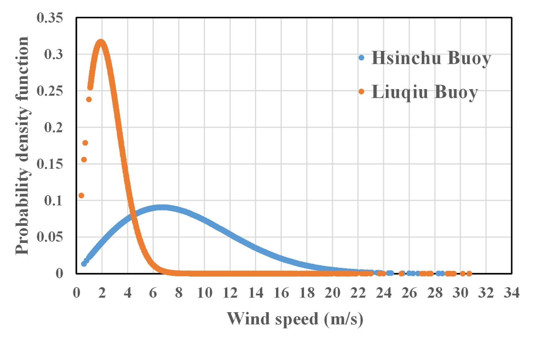
3.1. Estimation of Weibull Wind Speed Density
3.2. Fixed and Floating Wind Turbines
3.3. Wind Energy Conversion
4. Model Development and Evaluation
4.1. Establishment of the Recurrent Neural Network Model
- In an LSTM model, each LSTM layer comprises recurrently connected memory blocks, as proposed by Wollmer et al. [45]. These blocks consist of self-connected memory cells and three multiplicative gate units: input gates, output gates, and forget gates. Hochreiter and Schmidhuber [27] introduced this design to tackle the vanishing gradient problem in traditional RNNs. The key innovation of LSTM is the inclusion of a memory cell, enabling the establishment of persistent long-term dependencies [46]. This addresses the challenge of vanishing gradients in conventional RNNs. The orchestrated functioning of gate units within memory cells allows LSTM models to store and access information over extended periods [47], facilitating effective learning from sequences with long-range dependencies. For a deeper understanding, refer to the seminal work of Hochreiter and Schmidhuber [27].
- The GRU model, a variant of the LSTM neural network, consists of input, forget, and output layers [48]. In this architecture, the input gate regulates information influx, the forget gate manages memory content through recurrent connections, and the output gate influences data used in calculating the output activation, directing information flow [49]. Similar to LSTM, GRU features gating units that modulate information flow without a separate memory cell [50]. This design effectively captures patterns and dependencies in sequential data. For deeper insights, see Cho et al. [51] and Chung et al. [52].
- The stacked LSTM architecture refers to an LSTM model consisting of multiple LSTM layers, also known as deep LSTMs. Similar to the RNN model framework, the stacked LSTM model comprises multiple LSTM layers stacked before being passed to a dropout layer and an output layer for the final output.
4.2. Parameter Calibration
- For the parameter tuning of delay time in the models, testing starts with d = 1 h and progresses in 1-hour intervals up to a delay of 12 h. Figure 6 shows the RMSE errors under different delay times. The optimal delay time for the LSTM model at the Hsinchu Buoy remains at 10 h (Figure 6a), while for the GRU model, it ranges between 4 and 10 h (Figure 6b). For the Liuqiu Buoy, the LSTM model’s delay time ranges from 3 to 12 h (Figure 6c), and for the GRU model, it falls between 2 and 11 h (Figure 6d).
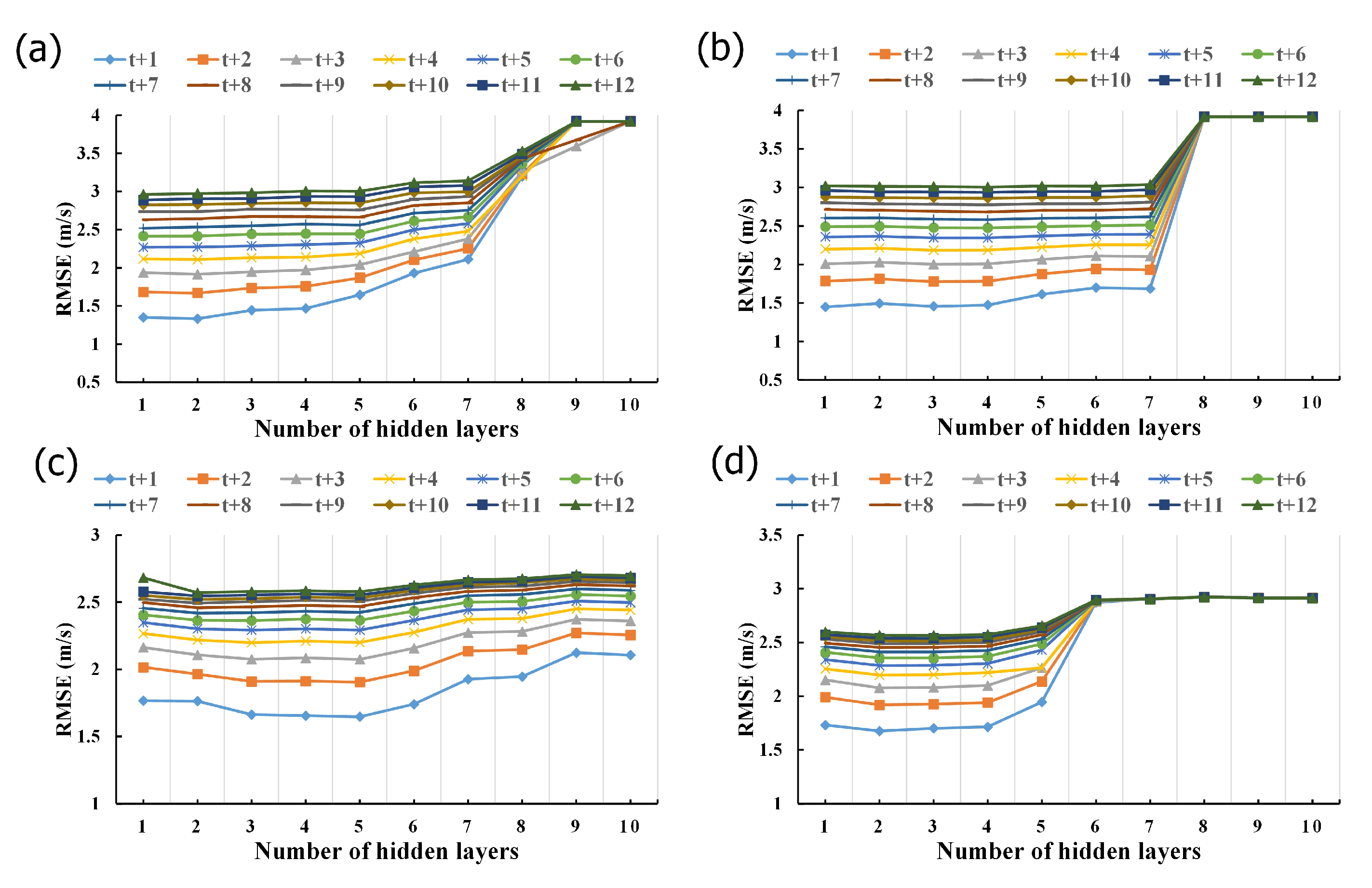
- For the number of hidden layers, the study explores 1 to 10 layers through trial and error. Figure 7 displays RMSE errors for different numbers of hidden layers. The optimal number of hidden layers for the LSTM model at the Hsinchu Buoy ranges between 1 and 2 layers, with 2 layers for t + 1 to t + 4 and 1 layer for t + 5 to t + 12. The optimal number of hidden layers for the GRU model is between 1 and 4 layers. For the Liuqiu Buoy, the optimal number of hidden layers for the LSTM model ranges between 2 and 5 layers, with 5 layers for t + 1 to t + 3 and t + 5, 3 layers for t + 4 and t + 6, and 2 layers for the rest. The optimal number of hidden layers for the GRU model ranges between 2 and 3 layers.
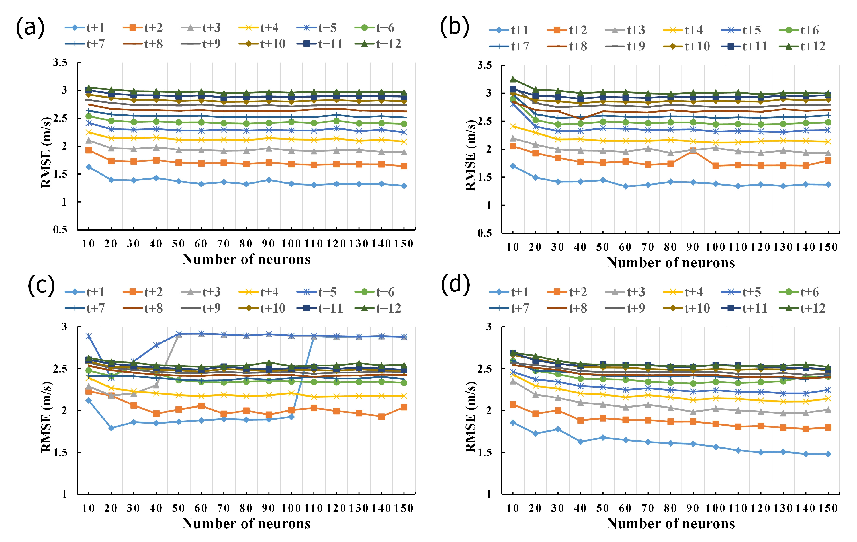
- The number of neurons in hidden layers significantly influences the model’s generalization. Too few neurons may lead to underfitting, while too many can cause overfitting. The study explores neuron counts from 10 to 150 in increments of 10. Figure 8 shows the results, indicating that for the LSTM model at Hsinchu Buoy, the optimal neuron count is 150, and for the GRU model, it ranges from 30 to 130. For Liuqiu Buoy, the LSTM model’s optimal range is 20 to 150, and the GRU model ranges from 130 to 150.
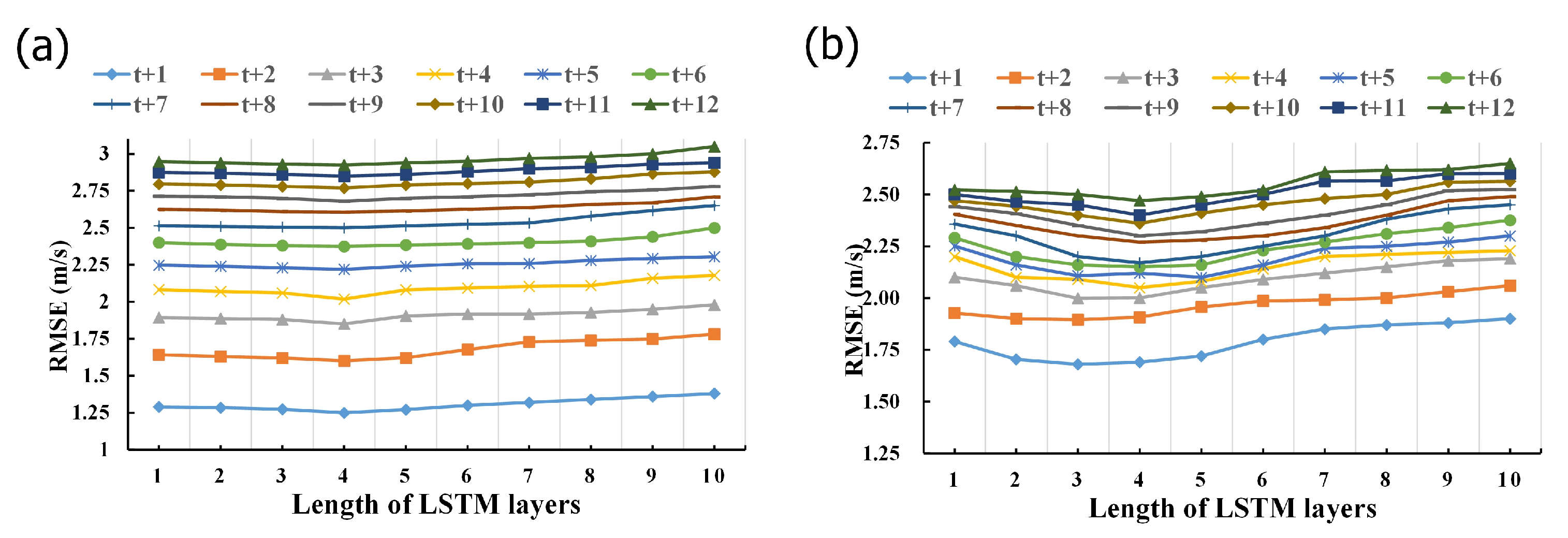
- Concerning the length of LSTM layers, the study investigates LSTM layers ranging from 1 to 10. Figure 9 illustrates the results, suggesting that for the stacked LSTM model at Hsinchu Buoy, the optimal number of LSTM layers falls within the range of 3 to 5. In the case of Liuqiu Buoy, the optimal range for the stacked LSTM model is identified as 2 to 5.
4.3. Test Results
5. Wind Rose Analysis and Seasonal Wind Speed Prediction Model
5.1. Seasonal Statistical Characteristics
5.2. Comparisons between Seasonal and Annual Models
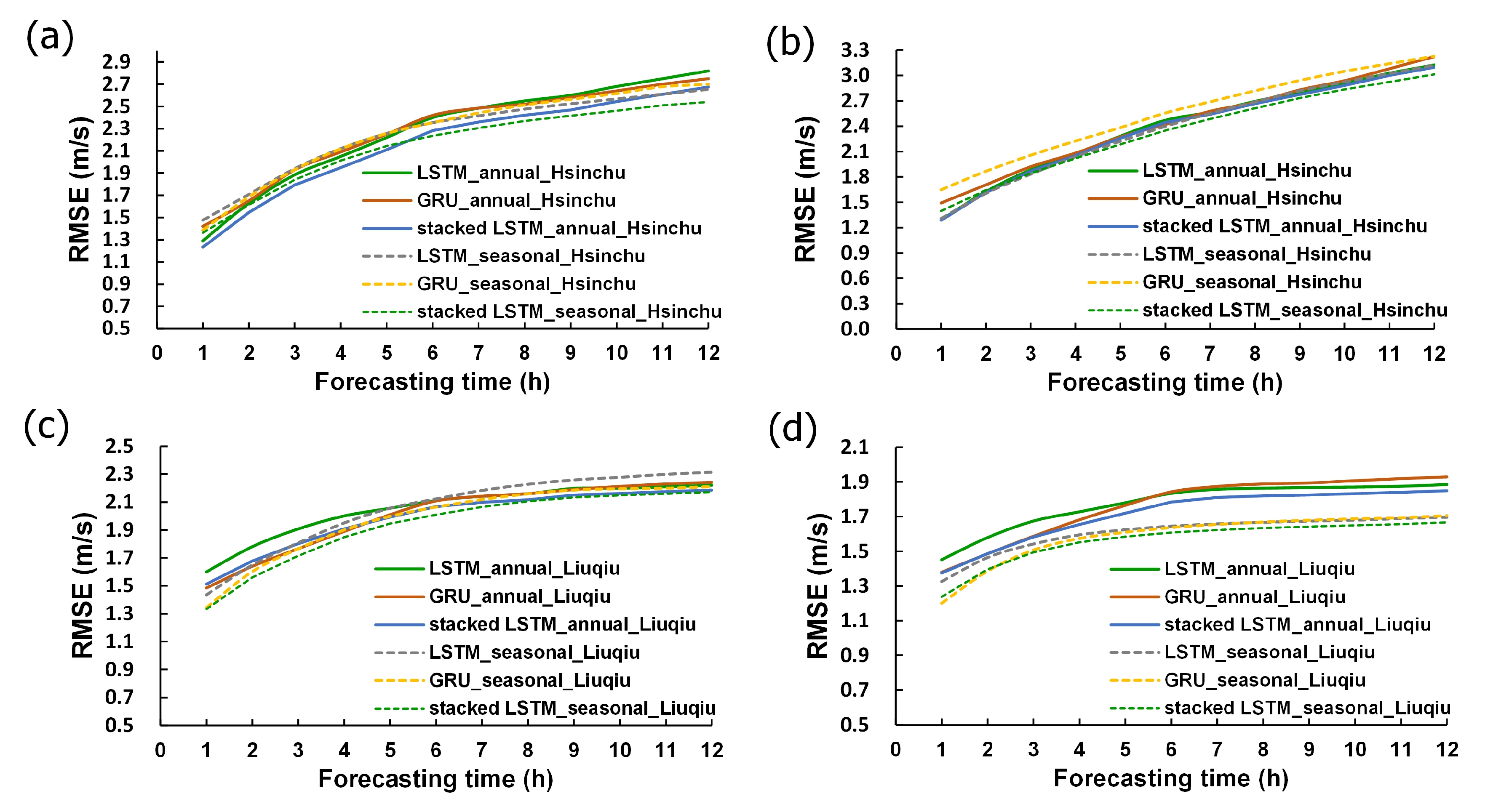
- Figure 15a shows that the seasonal model offshore Hsinchu performs worse than the annual model before t + 6 in summer, but after t + 6, the seasonal model’s error becomes lower. Hence, the annual model can be chosen before t + 6, and the seasonal model after t + 6.
- Figure 15b illustrates the non-summer results offshore Hsinchu. With the exception of a slightly larger error in the GRU seasonal model, both the LSTM annual model and GRU annual model exhibit similar errors. In comparison, the stacked LSTM seasonal model demonstrates the smallest error.
- Figure 15c presents the summer results offshore Kaohsiung. In the LSTM models, the annual model shows higher testing errors than the seasonal model before t + 6, and this situation reverses after t + 6. In the GRU models, the difference in testing errors between the annual and seasonal models is relatively small. In comparison to LSTM and GRU, the stacked LSTM demonstrates the smallest error.
- Figure 15d illustrates non-summer results offshore Kaohsiung. Overall, the annual-based model exhibits larger errors, while the seasonal-based model demonstrates smaller errors. The stacked LSTM shows satisfactory results in both the annual-based and seasonal-based models.
6. Real-Time Power Generation Assessment
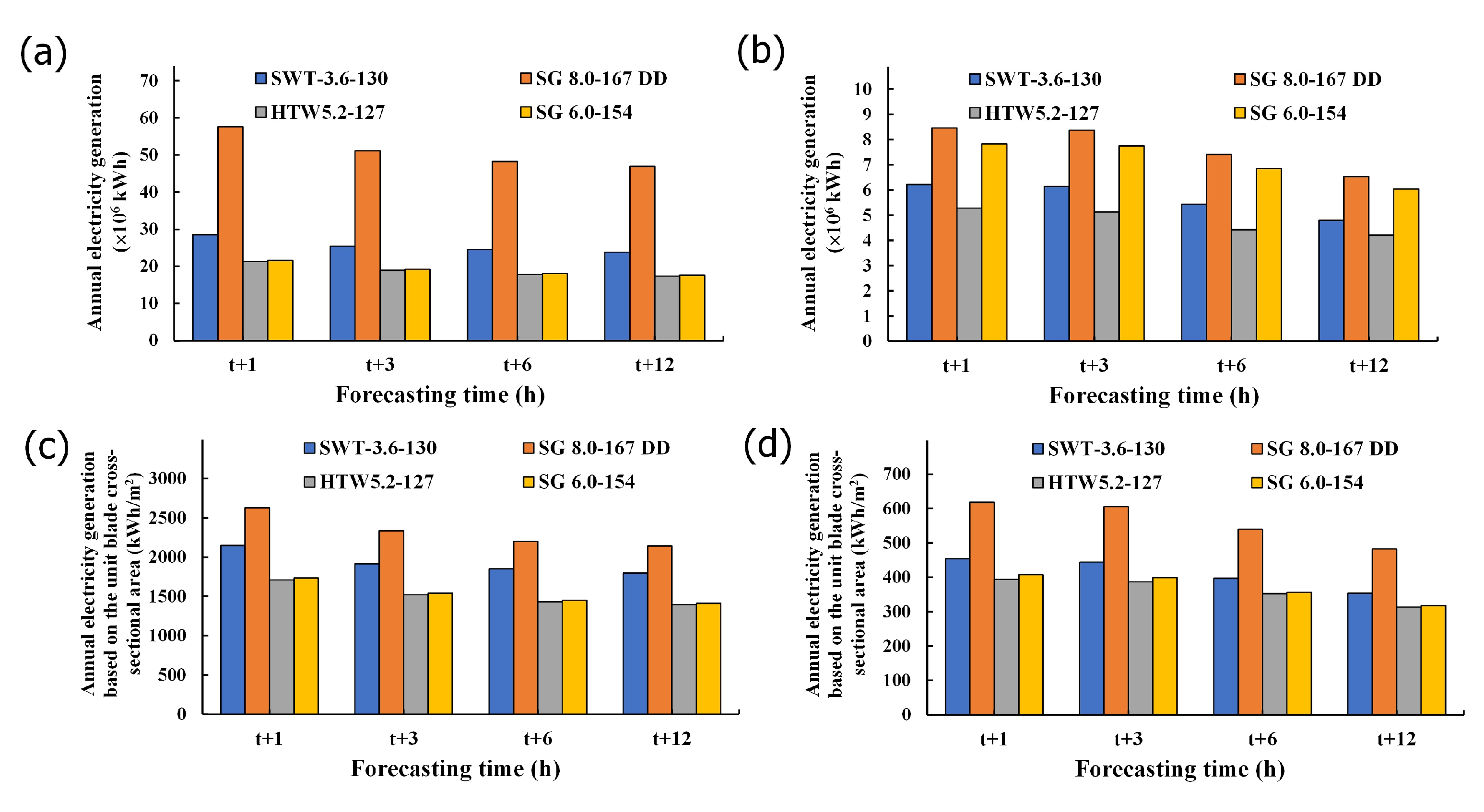
6.1. Annual Power Generation Forecast for Offshore Wind Turbines
6.2. Annual Power Generation per Unit Blade Swept Area
6.3. Discussion
7. Conclusions and Suggestions
7.1. Conclusions
- With the continuous growth of the global population, the demand for electricity is also on the rise, leading to a steady expansion of the global renewable energy market.
- Subsidies for renewable energy in advanced countries are trending towards stability or reduction, and countries are gradually introducing more competitive auction systems. Examining the current major global models for promoting renewable energy, these may include target setting, feed-in tariffs, electricity price differential subsidies, renewable energy ratios, green certificates, auction systems, and more.
- Local governments actively propose future development plans to expand the use of renewable energy in their regions. Globally, over 250 cities have committed to achieving a 100% renewable energy goal.
- The green supply chain is thriving, with companies increasingly demanding the procurement of renewable energy.
7.2. Limitations and Future Suggestions
Author Contributions
Funding
Institutional Review Board Statement
Informed Consent Statement
Data Availability Statement
Acknowledgments
Conflicts of Interest
References
- 4C Offshore. 2023. Global Wind Speed Rankings. Available online: http://www.4coffshore.com/windfarms/windspeeds.aspx (accessed on 1 October 2023).
- Energy Administration of Taiwan. 4-Year Wind Power Promotion Plan. 2017. Available online: https://www.moeaea.gov.tw/ECW/populace/content/ContentDesc.aspx?menu_id=5493 (accessed on 1 October 2023).
- Hennessey, J.P. Some aspects of wind power statistics. J. Appl. Meteorol. Climatol. 1977, 16, 119–128. [Google Scholar] [CrossRef]
- Corotis, R.B.; Sigl, A.B.; Klein, J. Probability models of wind velocity magnitude and persistence. Sol. Energy 1978, 20, 483–493. [Google Scholar] [CrossRef]
- Lalas, D.P.; Tselepidaki, H.; Theoharatos, G. An analysis of wind power potential in Greece. Sol. Energy 1983, 30, 497–505. [Google Scholar] [CrossRef]
- Altunkaynak, A.; Erdik, T.; Dabanlı, I.; Sen, Z. Theoretical derivation of wind power probability distribution function and applications. Appl. Energy 2012, 92, 809–814. [Google Scholar] [CrossRef]
- Fyrippis, I.; Axaopoulos, P.J.; Panayiotou, G. Wind energy potential assessment in Naxos Island, Greece. Appl. Energy 2010, 87, 577–586. [Google Scholar] [CrossRef]
- Zárate-Miñano, R.; Anghel, M.; Milano, F. Continuous wind speed models based on stochastic differential equations. Appl. Energy 2013, 104, 42–49. [Google Scholar] [CrossRef]
- Beaucage, P.; Lafrance, G.; Lafrance, J.; Choisnard, J.; Bernier, M. Synthetic aperture radar satellite data for offshore wind assessment: A strategic sampling approach. J. Wind. Eng. Ind. Aerodyn. 2011, 99, 27–36. [Google Scholar] [CrossRef]
- Oh, K.Y.; Kim, J.Y.; Lee, J.S.; Ryu, K.W. Wind resource assessment around Korean Peninsula for feasibility study on 100 MW class offshore wind farm. Renew. Energy 2012, 42, 217–226. [Google Scholar] [CrossRef]
- Ganea, D.; Amortila, V.; Mereuta, E.; Rusu, E. A joint evaluation of the wind and wave energy resources close to the Greek Islands. Sustainability 2017, 9, 1025. [Google Scholar] [CrossRef]
- González, A.; Pérez, J.C.; Díaz, J.P.; Expósito, F.J. Future projections of wind resource in a mountainous archipelago, Canary Islands. Renew. Energy 2017, 104, 120–128. [Google Scholar] [CrossRef]
- Chang, T.J.; Wu, Y.T.; Hsu, H.Y.; Chu, C.R.; Liao, C.M. Assessment of wind characteristics and wind turbine characteristics in Taiwan. Renew. Energy 2003, 28, 851–871. [Google Scholar] [CrossRef]
- Cheng, K.S.; Ho, C.Y.; Teng, J.H. Wind and sea breeze characteristics for the offshore wind farms in the central coastal area of Taiwan. Energies 2022, 15, 992. [Google Scholar] [CrossRef]
- You, Q.L.; Fraedrich, K.; Min, J.Z.; Kang, S.C.; Zhu, X.H.; Pepin, N.; Zhang, L. Observed surface wind speed in the Tibetan Plateau since 1980 and its physical causes. Int. J. Climatol. 2014, 34, 1873–1882. [Google Scholar] [CrossRef]
- Chen, L.; Li, D.; Pryor, S.C. Wind speed trends over China: Quantifying the magnitude and assessing causality. Int. J. Climatol. 2013, 33, 2579–2590. [Google Scholar] [CrossRef]
- Avila, D.; Marichal, G.N.; Hernández, A.; San Luis, F. Chapter 2—Hybrid renewable energy systems for energy supply to autonomous desalination systems on Isolated Islands. In Design, Analysis, and Applications of Renewable Energy Systems; Azar, A.T., Kamal, N.A., Eds.; Academic Press: Cambridge, MA, USA, 2021; pp. 23–51. [Google Scholar]
- Erdem, E.; Shi, J. ARMA based approaches for forecasting the tuple of wind speed and direction. Appl. Energy 2011, 88, 1405–1414. [Google Scholar] [CrossRef]
- Shukur, O.B.; Lee, M.H. Daily wind speed forecasting through hybrid KF-ANN model based on ARIMA. Renew. Energy 2015, 76, 637–647. [Google Scholar] [CrossRef]
- Leva, S.; Dolara, A.; Grimaccia, F.; Mussetta, M.; Ogliari, E. Analysis and validation of 24 hours ahead neural network forecasting of photovoltaic output power. Math. Comput. Simul. 2017, 131, 88–100. [Google Scholar] [CrossRef]
- Li, G.; Shi, J. On comparing three artificial neural networks for wind speed forecasting. Appl. Energy 2010, 87, 2313–2320. [Google Scholar] [CrossRef]
- Yang, L.; He, M.; Zhang, J.S.; Vittal, V. Support-vector-machine-enhanced markov model for short-term wind power forecast. IEEE Trans. Sustain. Energy 2015, 6, 791–799. [Google Scholar] [CrossRef]
- Liu, H.; Tian, H.Q.; Li, Y.F. Comparison of new hybrid FEEMD-MLP, FEEMD-ANFIS, Wavelet Packet-MLP and Wavelet Packet-ANFIS for wind speed predictions. Energy Convers. Manag. 2015, 89, 1–11. [Google Scholar] [CrossRef]
- Wang, H.Z.; Wang, G.B.; Li, G.Q.; Peng, J.C.; Liu, Y.T. Deep belief network based deterministic and probabilistic wind speed forecasting approach. Appl. Energy 2016, 182, 80–93. [Google Scholar] [CrossRef]
- Wang, H.Z.; Li, G.Q.; Wang, G.B.; Peng, J.C.; Jiang, H.; Liu, Y.T. Deep learning based ensemble approach for probabilistic wind power forecasting. Appl. Energy 2017, 188, 56–70. [Google Scholar] [CrossRef]
- Goh, S.L.; Chen, M.; Popović, D.H.; Aihara, K.; Obradovic, D.; Mandic, D.P. Complex-valued forecasting of wind profile. Renew. Energy 2006, 31, 1733–1750. [Google Scholar] [CrossRef]
- Hochreiter, S.; Schmidhuber, J. Long short-term memory. Neural Comput. 1997, 9, 1735–1780. [Google Scholar] [CrossRef] [PubMed]
- Liu, Y.; He, J.; Wang, Y.; Liu, Z.; He, L.; Wang, Y. Short-term wind power prediction based on CEEMDAN-SE and bidirectional LSTM neural network with Markov chain. Energies 2023, 16, 5476. [Google Scholar] [CrossRef]
- Shivam, K.; Tzou, J.C.; Wu, S.C. Multi-step short-term wind speed prediction using a residual dilated causal convolutional network with nonlinear attention. Energies 2020, 13, 1772. [Google Scholar] [CrossRef]
- Xiong, B.; Meng, X.; Wang, R.; Wang, X.; Wang, Z. Combined model for short-term wind power prediction based on deep neural network and long short-term memory. J. Phys. Conf. Ser. 2021, 1757, 012095. [Google Scholar] [CrossRef]
- Abdul Baseer, M.; Almunif, A.; Alsaduni, I.; Tazeen, N. Electrical power generation forecasting from renewable energy systems using artificial intelligence techniques. Energies 2023, 16, 6414. [Google Scholar] [CrossRef]
- Jaseena, K.U.; Kovoor, B.C. A hybrid wind speed forecasting model using stacked autoencoder and LSTM. J. Renew. Sustain. Energy 2020, 12, 023302. [Google Scholar] [CrossRef]
- Shahid, F.; Zameer, A.; Iqbal, M.J. Intelligent forecast engine for short-term wind speed prediction based on stacked long short-term memory. Neural Comput. Appl. 2021, 33, 13767–13783. [Google Scholar] [CrossRef]
- Kusiak, A.; Song, Z. Design of wind farm layout for maximum wind energy capture. Renew. Energy 2010, 35, 685–694. [Google Scholar] [CrossRef]
- Lackner, M.A.; Elkinton, C.N. An analytical framework for offshore wind farm layout optimization. Wind. Eng. 2007, 31, 17–31. [Google Scholar] [CrossRef]
- Shu, Z.R.; Li, Q.S.; Chan, P.W. Investigation of offshore wind energy potential in Hong Kong based on Weibull distribution function. Appl. Energy 2015, 156, 362–373. [Google Scholar] [CrossRef]
- SWT-3.6-130. Available online: https://en.wind-turbine-models.com/turbines/1468-siemens-swt-3.6-130 (accessed on 10 July 2023).
- SG 8.0-167 DD. Available online: https://www.siemensgamesa.com/products-and-services/offshore/wind-turbine-sg-8-0-167-dd (accessed on 10 July 2023).
- HTW5.2-127. Available online: https://www.thewindpower.net/turbine_en_1410_hitachi_htw5.2-127.php (accessed on 10 July 2023).
- SG 6.0-154. Available online: https://en.wind-turbine-models.com/turbines/1886-siemens-gamesa-sg-6.0-154 (accessed on 10 July 2023).
- Carrillo, C.; Obando Montaño, A.F.; Cidrás, J.; Díaz-Dorado, E. Review of power curve modelling for wind turbines. Renew. Sustain. Energy Rev. 2013, 21, 572–581. [Google Scholar] [CrossRef]
- Yeh, T.H.; Wang, L. A study on generator capacity for wind turbines under various tower heights and rated wind speeds using Weibull distribution. IEEE Trans. Energy Convers. 2008, 23, 592–602. [Google Scholar]
- Patel, M.R. Wind and Solar Power System; CRC Press LCC: New York, NY, USA, 1999. [Google Scholar]
- Khogali, A.; Albar, O.F.; Yousif, B. Wind and solar energy potential in Makkah (Saudi Arabia)-Comparison with Red Sea coastal sites. Renew. Energy 1991, 1, 435–440. [Google Scholar] [CrossRef]
- Wollmer, M.; Schuller, B.; Rigoll, G. Keyword spotting exploiting long short-term memory. Speech Commun. 2013, 55, 252–265. [Google Scholar] [CrossRef]
- Wei, C.C. Collapse warning system using LSTM neural networks for construction disaster prevention in extreme wind weather. J. Civ. Eng. Manag. 2021, 27, 230–245. [Google Scholar] [CrossRef]
- Wollmer, M.; Eyben, F.; Graves, A.; Schuller, B.; Rigoll, G. Bidirectional LSTM networks for context-sensitive keyword detection in a cognitive virtual agent framework. Cogn. Comput. 2010, 2, 180–190. [Google Scholar] [CrossRef]
- Wang, X.; Xu, J.; Shi, W.; Liu, J. OGRU: An optimized gated recurrent unit neural network. J. Phys. Conf. Ser. 2019, 1325, 012089. [Google Scholar] [CrossRef]
- Wu, W.; Liao, W.; Miao, J.; Du, G. Using gated recurrent unit network to forecast short-term load considering impact of electricity price. Energy Procedia 2019, 158, 3369–3374. [Google Scholar] [CrossRef]
- Dey, R.; Salem, F.M. Gate-variants of gated recurrent unit (GRU) neural networks. arXiv 2017, arXiv:1701.05923. [Google Scholar]
- Cho, K.; Van, M.B.; Gulcehre, C.; Bahdanau, D.; Bougares, F.; Schwenk, H.; Bengio, Y. Learning phrase representations using RNN encoder–decoder for statistical machine translation. arXiv 2014, arXiv:1406.1078. [Google Scholar]
- Chung, J.; Gulcehre, C.; Cho, K.H.; Bengio, Y. Empirical evaluation of gated recurrent neural networks on sequence modeling. arXiv 2014, arXiv:1412.3555. [Google Scholar]
- REN21. Renewables 2023 Global Status Report. 2023. Available online: https://www.ren21.net/gsr-2023 (accessed on 26 January 2024).
- Industrial Technology Research Institute. International Trends and Policies in Renewable Energy Development. 2023. Available online: https://www.re.org.tw/knowledge/more.aspx?cid=201&id=3966 (accessed on 26 January 2024).


| Attribute | Unit | Min–Max, Mean | |
|---|---|---|---|
| Hsinchu Station | Kaohsiung Station | ||
| Surface pressure | hPa | 964.6–1033.3, 1099.46 | 976.9–1030.9, 1012.28 |
| Sea level pressure | hPa | 967.8–1037.0, 1012.80 | 977.2–1031.3, 1012.67 |
| Avg wind speed | m/s | 0–12.7, 1.96 | 0–16.6, 2.10 |
| Avg wind direction | ° | 0–360, 114.05 | 0–360, 205.75 |
| Max avg wind speed | m/s | 0–15.1, 2.67 | 0–17.2, 2.76 |
| Max avg wind direction | ° | 0–360, 121.87 | 0–360, 217.89 |
| Peak gust speed | m/s | 0–36.7, 6.12 | 0–39.1, 4.89 |
| Peak gust direction | ° | 0–360, 139.61 | 0–360, 212.59 |
| Precipitation | mm | 0–375, 0.23 | 0–108, 0.22 |
| Duration of rainfall | h | 0–1, 0.97 | 0–1, 0.04 |
| Attribute | Unit | Min–Max, Mean | |
|---|---|---|---|
| Hsinchu Buoy | Liuqiu Buoy | ||
| Avg wind speed | m/s | 0.6–28.6, 6.76 | 0.4–30.7, 3.94 |
| Avg wind direction | ° | 0–360, 121.75 | 0–360, 214.87 |
| Gust wind speed | m/s | 1.1–38.2, 8.51 | 1.1–40, 5.23 |
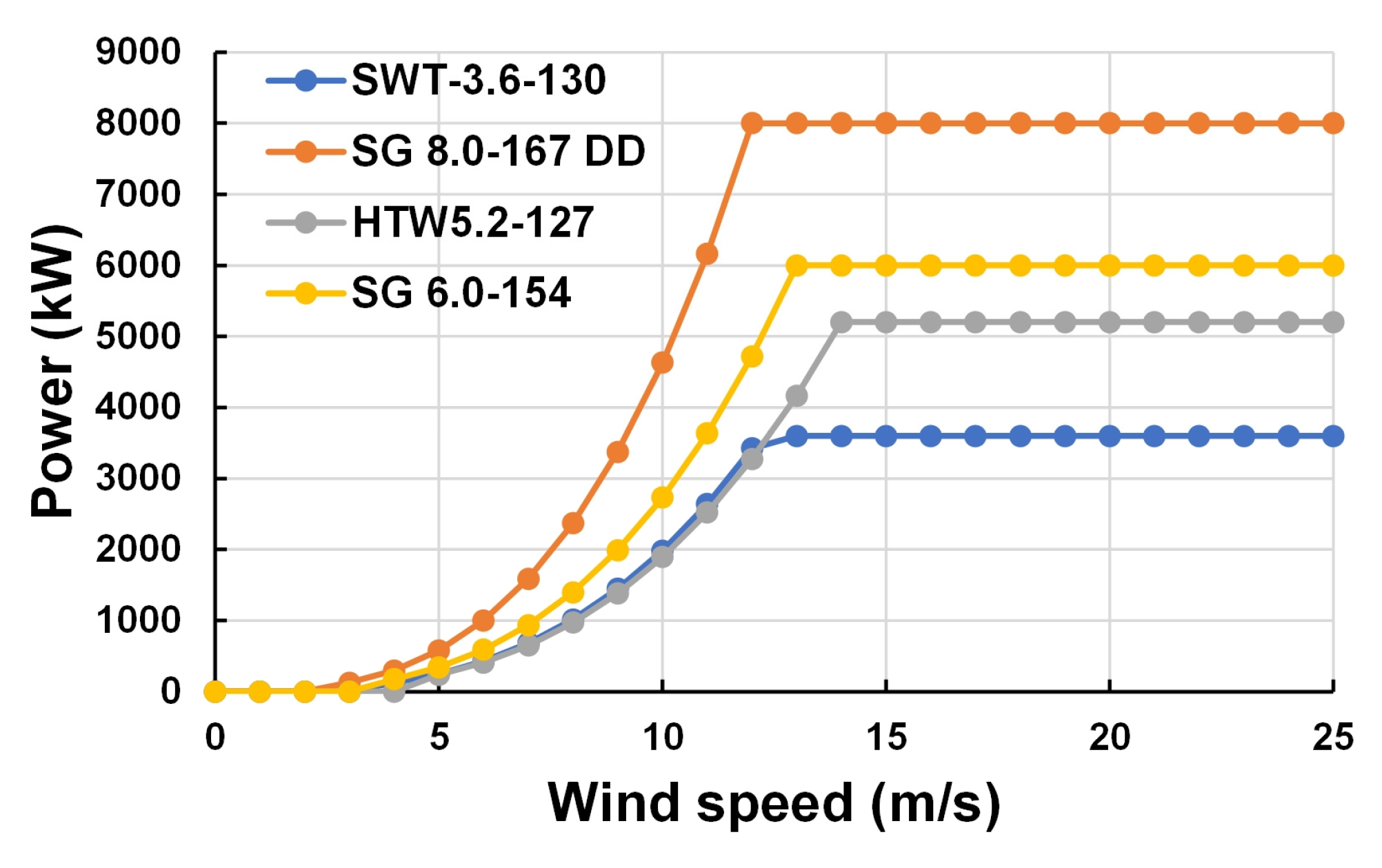
| Characteristics | SWT-3.6-130 | SG 8.0-167 DD | HTW5.2-127 | SG 6.0-154 |
|---|---|---|---|---|
| Rated power | 3600 kW | 8000 kW | 5200 kW | 6000 kW |
| Cut-in wind speed | 4.0 m/s | 3.0 m/s | 4.5 m/s | 4.0 m/s |
| Rated wind speed | 12.2 m/s | 12.0 m/s | 14.0 m/s | 13.0 m/s |
| Cut-out wind speed | 25.0 m/s | 25.0 m/s | 25.0 m/s | 25.0 m/s |
| Diameter | 130 m | 167 m | 127 m | 154 m |
| Swept area | 13,273 m2 | 21,904 m2 | 12,668 m2 | 18,627 m2 |
| Region | Hsinchu Offshore Area | Kaohsiung Offshore Area | ||
|---|---|---|---|---|
| Wind turbine model | SWT-3.6-130 | SG 8.0-167 DD | HTW5.2-127 | SG 6.0-154 |
| 0.244 | 0.345 | 0.244 | 0.239 | |
| Average wind speed at hub height | 10.30 m/s | 10.17 m/s | 5.77 m/s | 5.83 m/s |
| Annual power generation | 19 × 106 kWh | 42.7 × 10⁶ kWh | 3.1 × 10⁶ kWh | 4.7 × 10⁶ kWh |
Disclaimer/Publisher’s Note: The statements, opinions and data contained in all publications are solely those of the individual author(s) and contributor(s) and not of MDPI and/or the editor(s). MDPI and/or the editor(s) disclaim responsibility for any injury to people or property resulting from any ideas, methods, instructions or products referred to in the content. |
© 2024 by the authors. Licensee MDPI, Basel, Switzerland. This article is an open access article distributed under the terms and conditions of the Creative Commons Attribution (CC BY) license (https://creativecommons.org/licenses/by/4.0/).
Share and Cite
Wei, C.-C.; Chiang, C.-S. Assessment of Offshore Wind Power Potential and Wind Energy Prediction Using Recurrent Neural Networks. J. Mar. Sci. Eng. 2024, 12, 283. https://doi.org/10.3390/jmse12020283
Wei C-C, Chiang C-S. Assessment of Offshore Wind Power Potential and Wind Energy Prediction Using Recurrent Neural Networks. Journal of Marine Science and Engineering. 2024; 12(2):283. https://doi.org/10.3390/jmse12020283
Chicago/Turabian StyleWei, Chih-Chiang, and Cheng-Shu Chiang. 2024. "Assessment of Offshore Wind Power Potential and Wind Energy Prediction Using Recurrent Neural Networks" Journal of Marine Science and Engineering 12, no. 2: 283. https://doi.org/10.3390/jmse12020283
APA StyleWei, C.-C., & Chiang, C.-S. (2024). Assessment of Offshore Wind Power Potential and Wind Energy Prediction Using Recurrent Neural Networks. Journal of Marine Science and Engineering, 12(2), 283. https://doi.org/10.3390/jmse12020283