Typhoon Effects on Surface Phytoplankton Biomass Based on Satellite-Derived Chlorophyll-a in the East Sea During Summer

Abstract

The East Sea is a jointly managed maritime area of Korea, Russia, and Japan, where the frequency of strong typhoons is anticipated to increase with climate change, affecting its marine ecosystem and regional climate regulation. This study investigated the environmental and ecological impacts of summer typhoons entering the East Sea by analyzing satellite-derived chlorophyll-a (Chl-a) data, Argo float measurements, and ERA5 wind data. Our findings revealed that summer typhoons generally increased surface Chl-a concentrations by 65.4%, with typhoon intensity substantially influencing this process. Weak typhoons caused marginal Chl-a increases attributed to redistribution rather than nutrient supply, whereas normal and strong typhoons increased Chl-a through enhanced vertical mixing and nutrient upwelling in the East Sea. Stronger typhoons notably impacted the mixed layer depth and isothermal layer depth, leading to greater Chl-a concentrations within the strong wind radius. However, the increased Chl-a magnitude was lower than that of other strong typhoons in other regions. The East Sea uniquely responds to typhoons with fewer upper environment changes, possibly due to a stable barrier layer limiting vertical mixing. These findings underscore the importance of continuous monitoring and integrated observational methods in order to better understand the ecological effects of typhoons, particularly as their intensity increases with climate change.

1. Introduction

Global warming and climate change have increased the intensity and frequency of natural disasters worldwide. Recently, the frequency and intensity of typhoons affecting the seas around the Korean Peninsula have increased [1]. The Intergovernmental Panel on Climate Change report of 2015 indicates that rapidly rising sea surface temperatures around this region will impact typhoons significantly. A projected 2 °C global temperature increase due to climate change will lead to more frequent and severe typhoons [2,3], profoundly affecting the marine ecosystem in the seas surrounding South Korea. The Korea Meteorological Administration (KMA) reported 24 typhoons affecting South Korea between 2014 and 2022, with 13 categorized as strong intensity and three as very strong (extreme cases) [4]. Given the prevalence of high-intensity typhoons, understanding their effects on marine ecosystems around this region is crucial. Wang et al. [5] report that annual typhoon duration in the seas around South Korea, including the Yellow Sea, has increased by 143.3% over the past 40 years.

A direct effect of typhoons on the ocean is sea surface cooling, which decreases the Sea Surface Temperature (SST) when they pass over. This phenomenon has been studied since the early 1960s, primarily in the North Atlantic [6,7,8], and it mainly occurs in the mixed layer depth resulting in significant temperature variations (decreases ranging from 1 °C to 4 °C) [9]. Reportedly, it affects physical oceanographic changes and the habitat within the mixed layer [10]. Typhoons are associated with decreased sea temperatures and increased chlorophyll-a (Chl-a) concentrations in the seas surrounding South Korea, which serve as a proxy for phytoplankton biomass. In the South China Sea, Taiwan, China, typhoons cause an increase of >20% in new production [11]. Additionally, changes in nutrient concentrations (such as ${\mathrm{N}\mathrm{O}}_3^{-}$, and ${\mathrm{P}\mathrm{O}}_4^{3-}$) and Chl-a levels are observed when typhoons occur in areas near Taiwan [12]. As extreme weather events, typhoons can also substantially impact marine ecosystems and coastal areas by promoting the outbreak of biological disasters such as harmful algal blooms or accelerating their formation [13]. As primary producers, phytoplankton directly influences lower trophic-level dynamics and resource availability, and the crucial role of typhoons in marine ecosystems is their impact on Chl-a concentration, which serves as an indicator of phytoplankton biomass. Conversely, phytoplankton, associated with Chl-a, are highly sensitive to environmental factors, such as water temperature, salinity, light intensity, light period, ocean currents, and biological factors, including interspecies competition and predation by higher trophic-levels. Typhoon-induced effects have enhanced the diversity and abundance of fish species in the East Sea [14], highlighting the relevance of investigating typhoon effects on marine ecosystems [15,16,17].

The East Sea, known for the convergence of warm and cold ocean currents, has been the focus of various studies on marine environments and ecosystem changes, earning its reputation as a miniature ocean [18,19,20]. Recently, various physical, chemical, and biological changes have been observed due to climate change, particularly a decrease in primary productivity, raising concerns regarding the reduction in fishery resources [21,22,23,24,25]. However, the short-term increase in phytoplankton owing to the inflow of summer typhoons is expected to affect the proliferation of higher trophic-level organisms. In the Korean Peninsula, where typhoons mainly occur in summer, phytoplankton proliferation and primary productivity are typically low [25,26] caused by the seasonal thermocline, formed during the summer when surface water warming prevents nutrient-rich deep waters from reaching the euphotic zone [27]. Therefore, the influence of typhoons on waters around the Korean Peninsula, leading to surface cooling through Ekman pumping and phytoplankton increases through forced turbulence-induced entrainment, is expected to play a crucial role in post-typhoon marine ecosystem dynamics [28,29].

Research on marine ecosystems during the typhoon season was considered highly dangerous and often impossible because of weather conditions. Studies on the direct impacts of typhoons have been limited to coastal areas, with limited observations elsewhere, and therefore primarily focusing on the changes in coastal marine environments before and after typhoons, typhoon movement paths, and influence predictions [30]. However, recent advances in remote sensing data (satellite) technology now enable the assessment of changes in marine ecosystems before and after typhoon events, which were previously difficult to observe. Furthermore, Argo floats can operate under adverse weather conditions caused by typhoons and complement satellite data by measuring sea surface temperature and providing detailed analysis of upper ocean structure and typhoon-induced variability, thereby providing a more comprehensive assessment of the changes in marine ecosystems before and after these events.

Therefore, in this study, remote sensing (satellite) data, Argo float data and ERA5 reanalysis wind data were used to assess the impact of typhoon intensity on surface phytoplankton biomass in the East Sea during summer between 2018 and 2021. This research aims to understand the influence of typhoons on surface phytoplankton biomass (Chl-a) during summer, which is expected to increase in frequency and intensity in the marine ecosystem of the East Sea.

2. Data and Methods

2.1. Study Area and Typhoon Selection

The study area (34° N–45° N, 130° E–140° E) is shown in Figure 1. Our study focused on typhoons that passed through the East Sea during the summer months (July–September) from 2018 to 2021. Only typhoons with a satellite-derived composite data missing rate of ≤30%, specifically the difference (After–Before) images, were included in the analysis. We selected typhoons that traveled more than 200 km over the sea to analyze the radius of strong winds along their path. These thresholds were chosen to focus on typhoons that had sufficient time and distance to allow for the analysis of their strong wind radius. The typhoons were classified by intensity for a detailed analysis, according to the maximum wind speed per the KMA definition: ‘Weak’ (17 m/s–25 m/s), ‘Normal’ (25 m/s–33 m/s), ‘Strong’ (33 m/s–44 m/s), and ‘Very Strong’ (44 m/s–54 m/s), with latitude 34° N as the dividing line. Typhoon data were obtained from the KMA and were available at 6-h intervals from the entry point into the study area until their dissipation.

2.2. Data Collection: Satellite and Argo Float

Spatial analysis before and after the passage of typhoons in the study area was conducted using daily SST and Chl-a data from the Suomi National Polar-Orbiting Partnership Visible Infrared Imaging Radiometer Suite 4 km–Level 3 (accessed on 7 March 2023). We synthesized satellite images 7 days before and after each typhoon since variations in SST and Chl-a concentrations persist for 2–3 weeks [31,32,33]. One week of satellite imagery was used to capture the extreme effects of the typhoons. The Chl-a concentration is an indicator of phytoplankton biomass in the surface ocean [34,35,36]. However, the Chl-a concentration derived from satellite data may not always linearly reflect changes in phytoplankton biomass due to different photoacclimation [37,38]. Nevertheless, many previous studies have used Chl-a concentrations derived from ocean color to determine the variation in phytoplankton biomass and its relationship with environmental factors in the East Sea [39,40,41,42,43].

To determine the effect of typhoons on the water column during summer in the East Sea, we gathered vertical temperature profiles from the Argo float data obtained from the Global Data Assembly Center (accessed on March 7, 2023). Three Argo floats (2901783, 2901784, and 2901792) within the typhoon radius were analyzed using data collected 7 days before and after the typhoons, aligning with the observation periods of the satellite data. The locations of the Argo floats are shown in Figure 1, and information on the Argo floats is shown in

Table 1. The information of Argo floats’ and typhoons’ entry and exit dates.

No.			SOULIK	TAPA	MAYSAK HAISHEN (MH)
Float No.			2901784	2901783	2901792
Date	Typhoon	Entry	24-August-2018	23-September-2019	03-September-2020
		Exit	25-August-2018	23-September-2019	07-September-2020
	Argo	Before	23-August-2018	19-September-2019	29-August-2020
		After	30-August-2018	26-September-2019	12-September-2020
Location	Before	Latitude (°N)	38.726	36.878	36.769
		Longitude (°E)	131.139	134.125	130.92
	After	Latitude (°N)	38.612	36.911	36.875
		Longitude (°E)	131.671	134.361	131.559

.

2.3. Estimating the Typhoons’ Impact on the Environment in the East Sea

The Chl-a and SST values before and after typhoon passage were compared. The Haversine formula [44] was applied to calculate the spherical distance between the typhoon center and each pixel, and pixels located within the strong wind radius (from the typhoon center to its outer edge) were selected for analysis.

$$\mathrm{d}=2\mathrm{r}\mathrm{s}\mathrm{i}\mathrm{n}({\displaystyle \frac{∆\lambda }{2}})\sqrt{{sin}^2\left({\displaystyle \frac{\mathsf{\Delta }\lambda }{2}}\right)+\cos \left(\phi 1\right)\cos \left(\phi 2\right){sin}^2\left({\displaystyle \frac{\mathsf{\Delta }\lambda }{2}}\right)}$$

(1)

where d represents the distance between the two points, r is the radius of the Earth, Δλ is the difference in longitude, and φ1 and φ2 are the latitudes. This method allowed us to analyze the impact on the East Sea marine ecosystem within the typhoon radius.

To estimate the effects of typhoons on phytoplankton biomass, we collected Chl-a data for the strong wind radii of the typhoons. The strong wind radius of a typhoon is $\ge$15 m/s wind speed area from the center of the typhoon (KMA).

We compared the mixed layer depth (MLD), isothermal layer depth (ILD), and barrier layer (BL) before and after the typhoons in the target area using Argo float data specifically selected from within the strong wind radii of the typhoons to ensure relevance and accuracy in assessing their impact on the MLD. The MLD was determined as the depth where the density is higher, or the temperature is lower by a threshold value (ΔT = 0.2 °C) compared with the reference depth of 10 m [45,46,47]. The MLD was calculated using the following formula:

$$∆{\sigma }_{\theta }={\sigma }_{\theta }\left(T_{10}+∆{T,S}_{10},P_0\right)-{\sigma }_{\theta }\left(T_{10},S_{10},P_0\right)$$

(2)

where $∆{\sigma }_{\theta }$ represents the change in potential density, ${\sigma }_{\theta }\left(T_{10}\right)$ is the potential density at the reference depth of 10 m and $∆{T,S}_{10},P_0$ are the temperature and salinity difference at the reference depth and surface, respectively. The ILD represents the depth of the water column where the temperature remains relatively constant and is commonly used to identify thermocline structures. Argo float sensors can cause a 5 m error in identifying the MLD and ILD when using gradient criteria [48]. Therefore, similar to MLD, ILD was determined using a 0.5 °C temperature difference criterion compared with the temperature at a 10 m depth [49]. The BL, which lies between the MLD and ILD, represents a stratified layer that can inhibit vertical mixing. BL thickness is calculated as the difference between the ILD and MLD (BL = ILD − MLD), and its presence can influence heat and nutrient transport within the ocean [50,51,52].

To represent the vertical temperature structure of the water column, Argo temperature profiles collected before and after the typhoon’s passage were utilized. The temperatures were averaged from the surface to the Ekman Depth to assess the impact of vertical mixing.

Calculations of wind stress and subsequent Ekman Depth (D_E) relied heavily on accurate and high-resolution meteorological data. For this purpose, we used ERA5 hourly data from the European Center for Medium-Range Weather Forecasts (source: https://cds.climate.copernicus.eu/, accessed on 10 March 2021). The impact of typhoons on the sea surface can be described using D_E. D_E indicates the vertical region of the ocean affected by wind-driven surface water movement and can be calculated using the following formula [53]:

$$D_E={\displaystyle \frac{7.6}{\sqrt{sin\left|\phi \right|}}}{U}_{10}$$

(3)

$\phi$ represents the latitude, and $U_{10}$ is the wind speed. D_E was analyzed from 6 h before to 12 h after the typhoon when upwelling effects were most prominent [54].

Finally, the net heat flux ($Q_{net}$) can be calculated using the following equation:

$$Q_{net}=Q_{SW}-(Q_{LW}+Q_{LH}+Q_{SH})$$

(4)

where $Q_{SW}$ represents the net downward solar radiation (shortwave radiation), $Q_{LW}$ represents the net longwave radiation, $Q_{LH}$ denotes the latent heat flux associated with evaporation, and $Q_{SH}$ denotes the sensible heat flux caused by air–sea thermal convection. These heat flux components ($Q_{SW}, Q_{LW}, Q_{LH}, Q_{SH}$) were derived from ERA5 reanalysis data. When vertical and horizontal heat fluxes through the mixed layer are weak, the surface heat flux becomes the dominant factor driving SST variation [55]. All data processing and statistical analysis were performed using MATLAB (R2024a, MathWorks, Natick, MA, USA).

3. Results

3.1. The Features of Typhoons in the East Sea during Summer

Detailed information regarding the selected typhoons analyzed for their impact on the East Sea is presented in

Table 2. The information of typhoons during study period.

Name of Typhoon	Typhoon Lifetime	Duration [h]		Track Length [km]	Minimum Center Pressure [hPa]	Maximum Wind Speed [m/s]	Intensity	Missing Ratio of SST (%)	Missing Ratio of Chl-a (%)
		All	Ocean
SOULIK	16 August 2018. 09:00~25 August 2018 03:00	24	12	566	985	24	Weak	4.9	15.0
TAPA	19 September 2019 15:00~23 September 2019 09:00	9	6	481	985	27	Normal	8.8	22.0
MH	28 August 2020 15:00~7 September 2020 21:00	21	15	630	955	39	Strong	11.0	17.8

. The study encompasses five typhoons categorized by intensity: ‘Weak’ (SOULIK), ‘Normal’ (TAPA), and ‘Strong’ (MAYSAK AND HAISHEN, referred to as MH). Typhoon SOULIK, which occurred from 16 to 25 August 2018, lasted 24 h (including 12 h over the ocean) and traversed a track length of 566 km within the study area, with a minimum center pressure of 985 hPa, a maximum wind speed of 24 m/s, and a missing SST data ratio of 15.0%. Typhoon TAPA, which occurred between 19 and 23 September 2019, lasted 9 h (6 h over the ocean) and spanned a track length of 481 km, with a minimum center pressure of 985 hPa, a maximum wind speed of 27 m/s, and a missing SST data ratio of 5.6%. The combined Typhoons MAYSAK AND HAISHEN (MH) from 28 August to 7 September 2020, had a duration of 21 h (15 h over the ocean) and a track length of 630 km, with a minimum center pressure of 955 hPa, a maximum wind speed of 39 m/s, and a missing SST data ratio of 26.3%.

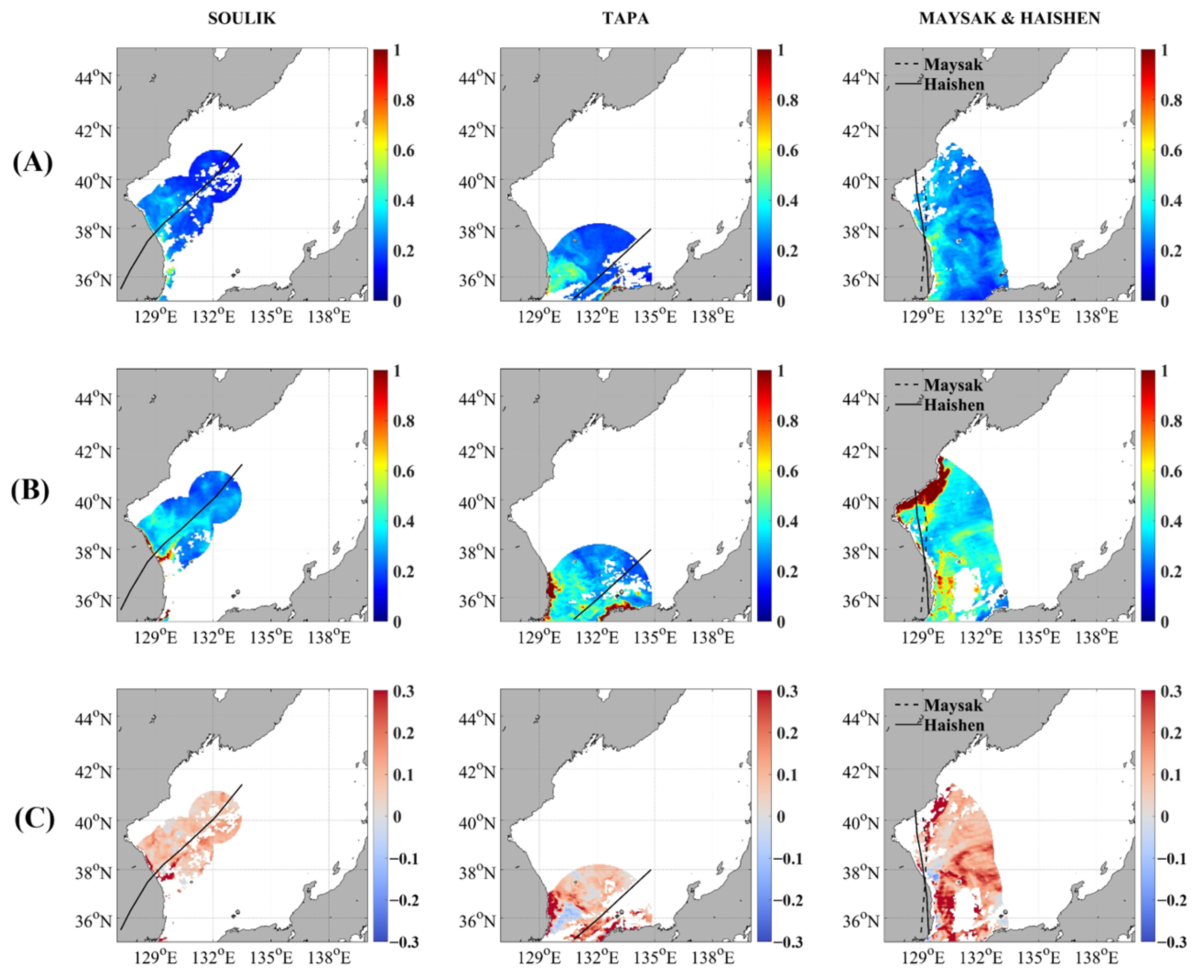
3.2. Chl-a Variability before and after the Typhoons

To determine the impact of typhoons on the East Sea, we examined differences in Chl-a. The spatial distribution of the Chl-a difference in the strong-wind radius of typhoons is shown in Figure 2, and the mean Chl-a in the strong-wind radius of typhoons is summarized in

Table 3. Chl-a concentration before, after, and difference between before and after typhoon in the strong wind radius of typhoon during the study period.

		SOULIK	TAPA	MH	Mean
Chl-a (mg m−3)	Before	0.22	0.28	0.28	0.26
	After	0.33	0.43	0.53	0.43
	Difference	0.11	0.15	0.25	0.17
	/%	/50.0%	/53.6%	/89.3%	/65.4%

. Chl-a levels in the East Sea increased after the typhoons, with higher intensity typhoons causing a greater increase. For the ‘Weak’ category, SOULIK had an average Chl-a of 0.22 mg m⁻³ before the typhoon, which increased to 0.33 mg m⁻³ after. Chl-a increased by 0.11 mg m⁻³ in the strong wind radius of SOULIK. The ‘Normal’ category typhoon, TAPA, had an average Chl-a of 0.28 mg m⁻³ before a typhoon, which increased to 0.43 mg m⁻³ after a typhoon. Chl-a increased by 0.15 mg m⁻³ in the strong wind radius of TAPA. For the ‘Strong’ typhoons, MH had an average Chl-a of 0.28 mg m⁻³ before a typhoon, which increased to 0.53 mg m⁻³ after a typhoon. Chl-a increased by 0.25 mg m⁻³ in the radius of MH. To determine the direct impact of typhoons on surface phytoplankton biomass, we examined the differences in Chl-a in the strong wind radii of typhoons (Figure 2C, Table 2). In all typhoons, Chl-a increased in the strong wind radius. The average Chl-a concentration was 0.26 mg m⁻³ before typhoons, which increased to 0.43 mg m⁻³ after, i.e., increasing by 0.17 mg m⁻³.

Chl-a increases within the strong wind radius were 0.11 mg m⁻³ (i.e., 50%), 0.15 mg m⁻³ (53.6%), and 0.25 mg m⁻³ (89.3%), for typhoons SOULIK, TAPA, and MH, respectively. In the strong wind radii of the typhoons, we found a dynamic variation in Chl-a after the typhoon. Indeed, within a strong wind radius, the Chl-a difference after the typhoons showed greater variation, depending on the intensity of the typhoons.

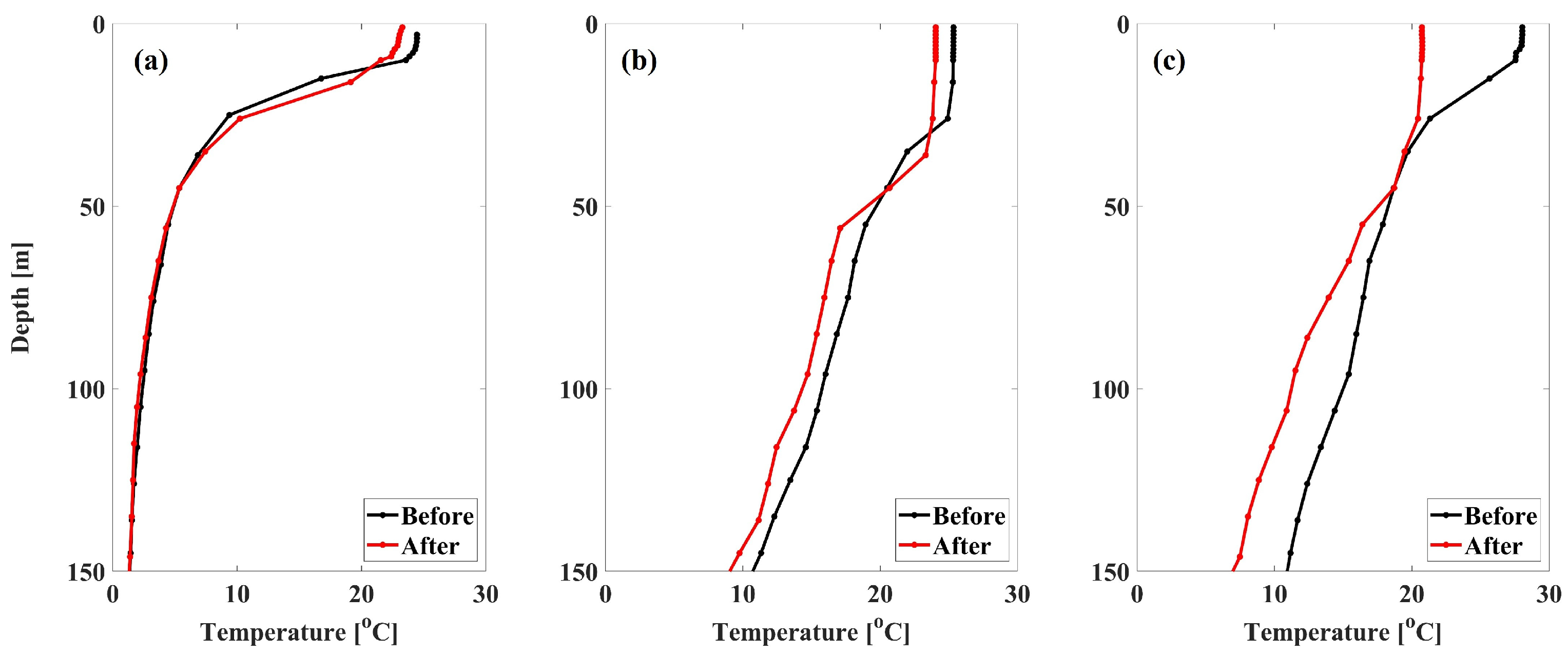
3.3. Differences in Satellite- and ARGO-Derived SST before and after the Typhoons in the East Sea

To assess the impact of typhoons on the East Sea, the average and difference in SST before and after typhoons with strong wind radii are presented in

Table 4. Comparison of SST and 0 m—D_E average temperature before and after typhoons’ passage in the East Sea Using satellite, Argo Float, and ERA5 data (in °C).

		Area	SOULIK	TAPA	MH	Mean
Satellite	Before	Strong wind radius	25.6	25.0	25.4	25.3
	After		23.7	23.4	21.2	22.8
	Difference		−1.9	−1.6	−4.1	−2.5
Argo float /∆T(DE)	Before		24.5/17.2	25.3/21.2	28/17.6	26.3/18.7
	After		23.3/17.3	24/20.3	20.7/14.8	23.7/17.5
	Difference		−1.2/0.1	−1.3/−0.9	−7.3/−2.8	−2.7/−1.2

. The table incorporates SST changes derived from satellite data, the Argo float, and ERA5 data. In all cases, the SST decreased after typhoons with a strong wind radius. For the ‘Weak’ category, SOULIK had an average SST of 25.6 °C before the typhoon, which decreased to 23.7 °C after, representing a reduction of 1.9 °C (Table 4). In the ‘Normal’ category, TAPA had an average SST of 25.0 °C before the typhoon, which decreased to 23.4 °C after, showing a reduction of 1.6 °C (Table 4). For the ‘Strong’ category, MH had an average SST of 25.4 °C before the typhoon, which decreased to 21.2 °C after, reflecting a reduction of 4.1 °C (Table 4). Similarly, the ARGO float data presented in Table 4 and Figure 3 show a consistent SST reduction after the typhoons. The ARGO SST decreased by 1.2 °C, 1.3 °C, and 7.3 °C after SOULIK, TAPA, and MH, respectively. Additionally, the Argo float temperature profiles averaged down to the Ekman Depth, with such averages representing vertical mixing processes, and indicated a 0.1 °C increase for SOULIK, a 0.3 °C decrease for TAPA, and a 2.8 °C decrease for MH (Table 4).

The Argo profile for SOULIK shows minimal changes, indicating weak vertical mixing. In contrast, the profile for TAPA demonstrates moderate vertical mixing, with the post-typhoon profile revealing a slightly deeper mixed layer. For MH, the profile highlights intense vertical mixing, characterized by substantial deepening of the mixed layer and pronounced surface cooling. Unlike the other typhoons, MH exhibits a thinning thermocline and a noticeable reduction in stratification, emphasizing its strong impact on the vertical structure of the water column.

To assess the impact of typhoons on ocean surface upwelling, we estimated D_E using surface wind data during the study period. D_E are presented in Figure 4 and

Table 5. Ekman Depth in strong wind radius of typhoons.

Category	SOULIK	TAPA	MH	Means
Mean Ekman Depth (DE) (m): strong wind radius	67	104	105	92

. In Figure 4, the darker the color, the greater the depth affected by wind-driven surface water movement. For the ‘Weak’ category SOULIK, D_E ranged from 18.7 m to 112.9 m within the strong wind radius. The ‘Normal’ category TAPA had D_E ranging from 16.4 m to 140.9 m within the strong wind radius. For the ‘Strong’ category MH, D_E ranged from 24.0 m to 121.1 m within the strong-wind radius. Overall, stronger typhoons were associated with deeper D_E, and larger areas were affected by considerable depth changes.

4. Discussion

4.1. The Typhoon Effects on Surface Phytoplankton Biomass in the East Sea

This study found that the phytoplankton biomass in the East Sea during summer was higher after typhoons than before. Satellite data before and after typhoons showed an increase in the Chl-a concentration in the surface layer in all areas influenced by the typhoons in the East Sea. Before typhoons, the average surface Chl-a was 0.26 mg m⁻³ within the strong wind radii, similar to the concentration of surface Chl-a in previous studies in the East Sea during summer (Table 3) [43,56,57]. Yamada et al. [43] reported that the surface Chl-a was approximately 0.2–0.3 mg m⁻³ in the East Sea from July to September. Additionally, Park et al. [57] reported a surface Chl-a < 0.16 mg m⁻³ in the East Sea. The phytoplankton biomass is low during summer owing to low nutrient conditions with strong stratification in the euphotic zone of the East Sea [56]. The observed increase in Chl-a concentration after the typhoon passage suggests that typhoons can alleviate nutrient limitations by promoting vertical mixing and upwelling, thereby enhancing primary productivity. Lim et al. [58] demonstrated that changes in the MLD significantly influence phytoplankton productivity, while Jeong [30] observed a modest increase in Chl-a concentration following Typhoon NABI (2005) in the Ulleung Basin, which was attributed to limited vertical mixing caused by the East Sea’s stratified conditions. These studies support our findings that the Chl-a response varies with typhoon intensity and movement speed. Lee et al. [27] further highlighted that the seasonal phytoplankton growth pattern differs between coastal and offshore areas in the Ulsan Bay (western part of the East Sea). During summer, strong thermal stratification limits phytoplankton growth in coastal waters, but typhoon-induced mixing temporarily enhances the nutrient supply, leading to increased Chl-a concentrations. This phenomenon aligns with the increase in surface Chl-a observed in this study after the passage of typhoons. Moreover, the relationship between subsurface chlorophyll maximum and nutrient concentrations in the East Sea underscores the critical role of typhoon-induced mixing. Kwak et al. [59] reported that nitrate concentrations in the East Sea are < 0.2 µM in the surface layer during summer, but they increase significantly below the MLD. Typhoons can disrupt strong stratification, lifting the subsurface chlorophyll maximum and nutrient-rich waters toward the surface, thus promoting phytoplankton growth. This explains the substantial Chl-a increase observed within the strong wind radii of typhoons in this study.

Indeed, the average Chl-a in the strong wind radii of typhoons increased to 0.43 mg m⁻³ after typhoons, rising by 0.17 mg m⁻³, with values ranging from 0.11 mg m⁻³ to 0.25 mg m⁻³ (Table 3). The increased surface Chl-a values were approximately 65.4%, ranging from 50.0% to 89.3% of Chl-a levels before the typhoons’ passages, within the strong wind radii. This increase in surface Chl-a can be attributed to two main factors [60]: first, mixing induced by typhoons brings nutrients from deeper layers to the surface, leading to photosynthetic blooms and subsequent net phytoplankton growth [61,62,63]; second, typhoons induce turbulent mixing that disrupts the SCM (Subsurface Chlorophyll Maximum) layer, leading to the upward displacement of chlorophyll maxima toward the surface [60,64,65]. This process involves physical redistribution rather than nutrient-driven growth, resulting in elevated surface Chl-a concentrations. However, the overall vertical nutrient availability and integrated Chl-a biomass remain largely unchanged [60]. Additionally, our study observed a decrease in temperature from the satellite and Argo floats in the strong wind radius during the passage of typhoons (Table 4). The average SST after typhoons decreased by 2.5 °C and 2.7 °C in the satellite and Argo float data, respectively. The Argo profiles further confirm that stronger typhoons weaken stratification due to intense mixing. Additionally, the temperature averaged over the Ekman Depth decreased by 1.2 °C as a result of the typhoons. This means that surface cooling and vertical mixing occurred during the typhoon passage. The decrease in SST following typhoon events can be explained by established cooling mechanisms in the East Sea [66]. The vertical mixing and entrainment of cooler subsurface water into the MLD, driven by the strong winds of typhoons, played a key role in reducing the SST, particularly evident in the ‘Strong’ category, where MH resulted in a 4.1 °C drop in SST within the strong wind radius based on satellite data, with Argo data showing a larger decrease of 7.3 °C at the surface and 2.8 at the Ekman Depth. Additionally, the cooling effect caused by typhoons is also influenced by air-sea heat fluxes. The $Q_{net}$ differences ($\left|∆Q_{net}\right|$) for SOULIK, TAPA, and MH were 133 W/m², 164 W/m², and 24.1 W/m², respectively. Although similar SST decreases were observed across the typhoons, the substantial $Q_{net}$ differences for SOULIK and TAPA suggest that air–sea heat fluxes played a significant role in driving SST reductions. Conversely, the minimal $Q_{net}$ difference for MH (24.1 W/m²) indicates that the observed SST decrease was primarily governed by vertical mixing and thermocline deepening, with limited contribution from air–sea interactions.

In the northwestern Pacific, water at 75 m depth can upwell 6 h before a typhoon of normal or greater intensity passes, and at 175 m depth, upwelling occurs 12 h after the typhoon passes [54]. Kwak et al. [59] reported that the nitracline in the Ulleung Basin, within the strong wind radius regions of typhoons SOULIK and MH, is located between 10 and 40 m. In contrast, Kodama et al. [67] reported that the nitracline in the region within the strong wind radius of typhoon TAPA ranges between 20 and 125 m. The D_E values of SOULIK and TAPA within their strong wind radii were insufficient to surpass the nitracline. However, the D_E (105 m) of Typhoon MH aligns with the upwelling mechanisms typically observed in the northwestern Pacific, suggesting that it was sufficient to penetrate the nitracline and induce nutrient upwelling. For the normal or stronger typhoons examined in this work, vertical mixing occurred down to D_E = 104.5 m average depth, resulting in an MLD increase of 5.4–8 m and an ILD increase of 5.4–18 m (

Table 6. MLD and ILD of typhoons before, after, and differences between before and after the Typhoon from Argo float.

Variables	Time	SOULIK	TAPA	MH
MLD (m) *	Before	9.9	18.4	9.9
	After	9.9	23.8	17.9
	Difference	-	5.4	8.0
ILD (m) *	Before	8.6	26.2	10.0
	After	6.5	31.6	28.0
	Difference	−1.9	5.4	18.0
Barrier layer thickness (m)	Before	-	7.8	0.1
	After	-	7.8	10.1
	Difference	-	-	10.0

* MLD: mixed layer depth, ILD: intermediate layer depth.

). During typhoon events, rapidly changing wind speeds and directions enhance turbulence and horizontal dispersion, primarily driven by wave orbital motion (WOM). WOM deepens the MLD but has a limited effect on deep vertical mixing, as its influence is typically confined to the upper ocean layer [68]. Additionally, the fast passage of typhoons further restricts the duration of wind stress, making it challenging for vertical mixing to penetrate deeper stratified layers. This aligns with findings by Zhang et al. [68], who demonstrated that surface wave-induced mixing redistributes surface energy without substantially affecting deeper layers.

This process redistributes Chl-a and the supply of nutrients, causing Chl-a concentrations to increase by 53.6–89.3%. Conversely, for weaker typhoons, vertical mixing occurs at an average depth of 67 m, with no change in MLD and ILD changes ranging from 1.9 m to 5.3 m, suggesting a 50% increase in Chl-a. It was more likely due to processes of SCM Chlorophyll redistribution rather than nutrient supply. The SCM typically appears in the 30–40 m water column of the East Sea [69,70]. The depth of the SCM has a strong relationship with the nitracline depth owing to the nutrient supply from deep water [26,70]. The nitracline, characterized by a rapid change in nutrient concentration, serves as a boundary between nutrient-depleted surface waters and nutrient-rich deep waters, providing a nutrient source that supports phytoplankton growth in the lower euphotic zone [71]. At this depth, phytoplankton either grow actively due to nutrient availability or increase their chlorophyll content per cell to adapt to lower light levels, resulting in the formation of the SCM [72]. Additionally, stable stratification reduces the sedimentation rate of phytoplankton, allowing them to accumulate at this depth, which further reinforces the SCM layer [73]. Kwak et al. [59] reported that the nitrate concentrations in the surface layer are <0.2 µM in the East Sea during summer. The nitrate concentration gradually increases below the MLD (75 m) in the East Sea. The surface Chl-a concentration in the East Sea during summer is lower because strong stratification restricts mixing in the water column. This blocks nutrient supply from deep water to surface water during summer [27,56]. The average D_E of the radial typhoons was 92 m in the East Sea (Table 5), indicating substantial mixing in the water column down to approximately 92 m. Consequently, typhoons can break the strong stratification of surface water during summer. This mixing can supply nutrients and Chl-a to the surface water. This is the main cause of phytoplankton biomass increases in the strong wind radii of typhoons.

To evaluate the effects of typhoon displacement speed on phytoplankton biomass in the East Sea, we estimated the movement speed of typhoons based on the distance traveled and duration. The movement speeds were 47.2, 80.2, and 42 km/h for SOULIK, TAPA, and MH, respectively. The intense but slow-moving speed MH had the strongest effect on surface phytoplankton biomass (89.3% Chl-a increase after typhoon), while TAPA, with normal intensity and fastest moving speed, had a medium effect (53.6% Chl-a increase). SOULIK, with weak intensity and slow movement speed, had a low effect (50.0% Chl-a increase). Despite the differing intensities of SOULIK and TAPA, their effects on phytoplankton biomass were comparable. This suggests that slow-moving typhoons have a more prolonged impact on vertical mixing and nutrient upwelling [74,75], which ultimately enhances phytoplankton growth more effectively. Therefore, both the intensity and movement speed of typhoons must be considered when evaluating their effects on the East Sea.

4.2. Comparison of the Typhoon Effects Between This Study and Previous Studies

To compare the effects of typhoons on phytoplankton biomass, we reviewed previous studies detailing variations in surface Chl-a during typhoons (Table 7). Studies have provided insight into the influence of intense typhoons on Chl-a concentrations in different regions. Girishkumar et al. [76] investigated the effects of Tropical Cyclone (TC) Hudhud in October 2014 as it passed through the Bay of Bengal, revealing that Chl-a concentrations increased from 0.15 mg m⁻³ to 3.6 mg m⁻³, based on data from Bio-Argo floats deployed in the central part of the ocean. Although TC Hudhud had not reached the intensity levels required for classification as a ‘Weak’ category under KMA standards, it had a notably greater impact on Chl-a concentrations than storms classified under the ‘Weak’ category in our study.

Babin et al. [32] reported that after the passage of the ‘Normal’ category Hurricane Michael in 2000, surface Chl-a concentrations increased from 0.08 mg m⁻³ to 0.14 mg m⁻³, a 79.9% increase. Similarly, another study [11] found that after the passage of the ‘Strong’ category Typhoon Kai-Tak in 2000, surface Chl-a concentrations increased 30-fold.

Further studies yielded similar results. Studies [77,78] documented that after the passage of the ‘Strong’ category Typhoon Damrey in 2005, surface Chl-a concentrations increased by 577% and 771%, respectively. Meanwhile, Walker et al. [79] found that after the passage of the ‘Very Strong’-category Hurricane Ivan (2004), Chl-a concentrations increased by 312%. Reportedly, [80] after the passage of the ‘Very Strong’-Category Typhoon Parma in 2009, Chl-a concentrations increased by 812%, demonstrating the significant influence intense storms can have on marine productivity. These studies indicate that the Chl-a concentrations in other regions exhibit more dynamic changes than those in our study area.

In contrast to previous research results, the fluctuations in phytoplankton biomass in our study were lower, ranging from 50% to 89.3%. Previous studies conducted around the Korean Peninsula have shown similar findings, with Son et al. [33] reporting increased Chl-a concentration from 0.29 mg m⁻³ to 0.64 mg m⁻³ after the passage of the ‘Normal’ category Typhoon Megi (2004). Similarly, Jeong [30] observed that the ‘Strong’ category Typhoon Navi (2005) resulted in a smaller increase in Chl-a concentrations, rising from 0.27 mg m⁻³ to 0.31 mg m⁻³ around the Ulleung Basin, which was along the typhoon’s path. Consequently, the environmental impacts of typhoons entering the East Sea appears to be relatively weaker than those occurring in other regions.

Table 7. The typhoons’ effects on surface phytoplankton biomass from previous studies.

Location	Typhoon			Chl-a (mg m−3)			Source
	Name	Date	Intensity	Before	After	Change (%)
Bay of Bengal	Hudhud	Oct 2014	TC *	0.15	3.6	2300	Giridhkumar et al. [76]
North Atlantic Ocean	Michael	Sep 2000	Normal	0.08	0.14	79.9	Babin et al. [32]
South Taiwan, Sea	Kai-Tak	Jul 2000	Strong	≤0.1	3.2 ± 4.4	3100	Lin et al. [11]
South Taiwan, Sea	Damrey	Sep 2005	Strong	0.16	1.05	577	Zheng and Tang. [77]
				0.07	0.61	771	Pan et al. [78]
Gulf of Mexico	Ivan	Sep 2004	Very Strong	0.24	0.99	312	Walker et al. [79]
South Taiwan, Sea	Parma	Oct 2009	Very Strong	0.08	0.73	812	Zhao et al. [80]
East Sea	Megi	Aug 2004	Normal	0.29	0.64	118	Son et al. [33]
East Sea	Navi	Oct 2013	Strong	0.27	0.31	12	Jeong [30]

* “Tropical Cyclone (TC)” refers to storms that have not yet reached the intensity levels required for classification as a ‘Weak’ category Typhoon under KMA standards.

Table 7. The typhoons’ effects on surface phytoplankton biomass from previous studies.

Location	Typhoon			Chl-a (mg m−3)			Source
	Name	Date	Intensity	Before	After	Change (%)
Bay of Bengal	Hudhud	Oct 2014	TC *	0.15	3.6	2300	Giridhkumar et al. [76]
North Atlantic Ocean	Michael	Sep 2000	Normal	0.08	0.14	79.9	Babin et al. [32]
South Taiwan, Sea	Kai-Tak	Jul 2000	Strong	≤0.1	3.2 ± 4.4	3100	Lin et al. [11]
South Taiwan, Sea	Damrey	Sep 2005	Strong	0.16	1.05	577	Zheng and Tang. [77]
				0.07	0.61	771	Pan et al. [78]
Gulf of Mexico	Ivan	Sep 2004	Very Strong	0.24	0.99	312	Walker et al. [79]
South Taiwan, Sea	Parma	Oct 2009	Very Strong	0.08	0.73	812	Zhao et al. [80]
East Sea	Megi	Aug 2004	Normal	0.29	0.64	118	Son et al. [33]
East Sea	Navi	Oct 2013	Strong	0.27	0.31	12	Jeong [30]

* “Tropical Cyclone (TC)” refers to storms that have not yet reached the intensity levels required for classification as a ‘Weak’ category Typhoon under KMA standards.

According to Wang et al. [48], stratification occurs when the thermocline (ILD) is deeper than the MLD, primarily due to salinity differences within the thermocline. This stratification forms a BL that prevents vertical mixing and inhibits the upwelling of nutrient-rich water. They reported that in the Northwest Pacific during summer, a 5–15 m BL can impede the upwelling of thermocline water caused by typhoons. Similarly, based on the data in Figure 3 and Table 6, the range of BL thickness in our study was determined to be between 0.1 and 10.1 m. However, since the Argo data were not collected immediately after typhoon events and the depth intervals of Argo measurements are typically 2–20 m, the BL depth in the East Sea may be underestimated. Wu and Chen [81] observed that the MLD measured by the Argo float reaches its maximum immediately after a typhoon passes and typically recovers within 6 days. In our study, observations of the Argo float, which were taken on average 4.8 days after the typhoon, likely reflect a shallower MLD and ILD due to this recovery process. Considering that the average MLD in summer is 37.3 m in the Northwest Pacific [82] and 12 m in the East Sea [58], the BL in the East Sea is expected to be thicker. The passage of SHANSHAN, a strong typhoon, through the East Sea resulted in changes in Chl-a concentrations ranging from 0.3 mg m⁻³ to 1.0 mg m⁻³ [83], which are encompassed by the broader range of our findings (−0.8 mg m⁻³ to 4.8 mg m⁻³; Figure 2). Therefore, changes in SST and Chl-a in the East Sea are smaller than those in other regions affected by typhoons. During the study period, the intensity and duration of typhoons entering the East Sea were insufficient to fully disrupt the BL. Although the D_E values indicate that vertical mixing temporarily exceeded the nitracline depth, this effect was transient and did not lead to a complete breakdown of stratification. Consequently, oceanic responses remained weaker overall, with only surface mixing dominating most of the observed changes. However, with the projected increase in the frequency and intensity of super typhoons owing to climate change [84], future storms may have a more profound impact on the East Sea. Zhang et al. [85] suggested that near the center of more intense typhoons, stronger winds can either deepen the MLD, weaken or remove the BL, or thicken it under certain conditions. This intensifies nutrient upwelling, resulting in increased phytoplankton biomass. Furthermore, organic matter, a crucial food source for deep-sea ecosystems, originates from primary production at the surface and is transported to the seabed through the food web during phytoplankton blooms [86,87]. Typhoon-induced nutrient upwelling can enhance this process, impacting the availability of nutrients and subsequently influencing the distribution of demersal fish [87,88]. In addition, habitat water temperature changes, particularly those induced by typhoons, are among the most critical factors influencing the behavior and distribution of fishery resources [89,90]. Short-term shifts in oceanic conditions caused by typhoons can significantly disrupt these dynamics, altering fish movement and availability. If future storms follow abnormal paths and affect the East Sea for longer durations, the region may experience more significant biological responses. However, the full extent of these processes is complex and warrants further investigation to understand fully how these dynamics evolve under changing climates.

5. Summary and Conclusions

This study determined the variations in SST, water column temperature, and phytoplankton biomass during typhoons entering the East Sea using satellite-derived Chl-a concentrations. We utilized Chl-a, SST, Argo float profiles, ERA5 wind and surface heat flux data collected between 2018 and 2022. To investigate the physical drivers of Chl-a variability during typhoon events, vertical mixing metrics, such as D_E, MLD, and ILD, were calculated. Chl-a concentration increased by approximately 65.4% in the East Sea during the typhoon passage, with variations linked to typhoon intensity. For typhoons of normal or greater intensity, the D_E, MLD, and ILD increased by an average of 104.5 m, 29–81%, and 21–180%, respectively, causing strong vertical mixing that led to a 53.6–89.3% increase in Chl-a concentrations. Conversely, for weaker typhoons, the D_E, MLD, and ILD changed by 67 m, 0%, and −24%, respectively, with limited vertical mixing resulting in a Chl-a increase of only 50%. Additionally, slow-moving typhoons, even those with similar intensities, had a more substantial effect on surface Chl-a concentration changes. In the East Sea, the BL suppressed vertical mixing, limiting nutrient supply and physical changes, which resulted in smaller Chl-a variations compared to other regions. Our study provides insight into the variations in phytoplankton biomass driven by typhoon intensity and moving speed, highlighting that stronger and slower-moving typhoons have a greater impact on the East Sea marine ecosystem. Nevertheless, the marine ecosystem response to typhoons is driven by complex mechanisms, and these findings are subject to certain limitations.

Although this study utilized satellite-derived Chl-a concentration as an indicator of phytoplankton biomass to evaluate the effects of typhoons in the East Sea, it is important to note that Chl-a may not always linearly correspond to phytoplankton biomass due to processes such as photoacclimation. While this study provides valuable insights, further research incorporating in situ measurements or additional approaches is needed to more accurately quantify the relationship between Chl-a and actual phytoplankton biomass. Additionally, the depth intervals of Argo measurements (2–20 m) introduce uncertainty in estimating the BL depth, which could influence the interpretation of vertical mixing processes and which warrants further investigation. Continuous research and monitoring using tools such as underwater gliders, BioGeoChemical Argo floats, and in situ observations are necessary for a deeper understanding of these complex interactions.

To further advance our understanding of marine ecosystem responses to typhoons, we plan to extend the study period and region in future research to analyze a broader range of typhoon cases. Moreover, we will incorporate key factors, such as typhoon wind speed, displacement velocity, and stratification parameters (e.g., Brunt–Väisälä frequency), into our analysis to better understand typhoon-induced mixing processes.

References

1. Kim, T.; Kim, E.; Lee, M.; Cha, D.H.; Lee, S.M.; Lee, J.; Boo, K.O. Characteristics of tropical cyclones over the western North Pacific related to extreme ENSO and a climate regime shift in sub-seasonal forecasting with GloSea5. Clim. Dyn. 2023, 61, 2637–2653. [Google Scholar] [CrossRef]
2. Korea Meteorological Administration. Korea Climate Change Assessment Report. 2020; Korea Meteorological Administration: Seoul, Republic of Korea, 2020; p. 29. [Google Scholar]
3. Kim, H.J.; Kim, D.B.; Jeong, O.J.; Moon, Y.S. The Moving Speed of Typhoons of Recent Years (2018–2020) and Changes in Total Precipitable Water Vapor Around the Korean Peninsula. J. Korean Earth Sci. Soc. 2021, 42, 264–277. [Google Scholar] [CrossRef]
4. Korean Meteorological Administration. Typhoon History and Statistics. Available online: https://www.weather.go.kr/w/typhoon/typ-history.do (accessed on 8 September 2023).
5. Wang, Z.; Bai, Y.; He, X.; Wu, H.; Bai, R.; Li, T.; Zhu, B.; Gong, F. Assessing the effect of strong wind events on the transport of particulate organic carbon in the Changjiang River estuary over the last 40 years. Remote Sens. Environ. 2023, 288, 113477. [Google Scholar] [CrossRef]
6. Jordan, C.L. On the influence of tropical cyclones on the sea surface temperature. In Proceedings of the Symposium on Tropical Meteorology; Hutchings, J.W., Ed.; New Zealand Meteorological Service: Wellington, New Zealand, 1964; pp. 614–622. [Google Scholar]
7. Pudov, V.D.; Varfolomeyev, A.A.; Fedorov, K.N. Vertical structure of the wake of a typhoon in the upper ocean. Oceanol. Acad. Sci. USSR 1978, 18, 142–146. [Google Scholar]
8. Taira, K.; Kitagawa, S.; Otobe, H.; Asai, T. Observation of temperature and velocity from a surface buoy moored in the Shikoku Basin (OMLET-88)—An oceanic response to a Typhoon. J. Oceanogr. 1993, 49, 397–406. [Google Scholar] [CrossRef]
9. Hong, C.H. A numerical study of sea surface cooling with the passage of typhoon Abby in the Northwestern Pacific. Korean J. Fish. Aquat. 2008, 41, 518–524. [Google Scholar] [CrossRef]
10. Hong, C.H.; Masuda, A. Temperature Variations in the Mixed Layer with the Passage of Typhoons Using One-Dimensional Numerical Model. Korean J. Fish. Aquat. Sci. 2018, 51, 107–112. [Google Scholar] [CrossRef]
11. Lin, I.; Liu, W.T.; Wu, C.C.; Wong, G.T.F.; Hu, C.M.; Chen, Z.Q.; Liang, W.D.; Yang, Y.; Liu, K.K. New evidence for enhanced ocean primary production triggered by tropical cyclone. Geophys. Res. Lett. 2003, 30, 1718–1722. [Google Scholar] [CrossRef]
12. Chen, C.-T.A.; Liu, C.-T.; Chuang, W.; Yang, Y.; Shiah, F.-K.; Tang, T.; Chung, S. Enhanced buoyancy and hence upwelling of subsurface Kuroshio waters after a typhoon in the southern East China Sea. J. Mar. Syst. 2003, 42, 65–79. [Google Scholar] [CrossRef]
13. Yao, L.; He, P.; Xia, Z.; Li, J.; Liu, J. Typical Marine Ecological Disasters in China Attributed to Marine Organisms and Their Significant Insights. Biology 2024, 13, 678. [Google Scholar] [CrossRef] [PubMed]
14. Jung, Y.W.; Kim, B.S.; Jung, H.K.; Lee, C.I. Distributional Changes in Fishery Resource Diversity Caused by Typhoon Pathways in the East/Japan Sea. Fishes 2023, 8, 242. [Google Scholar] [CrossRef]
15. Thompson, P.A.; Bonham, P.I.; Swadling, K.M. Phytoplankton blooms in the Huon Estuary, Tasmania: Top-down or bottom-up control? J. Plankton Res. 2008, 7, 735–753. [Google Scholar] [CrossRef]
16. Guinder, V.A.; Popovich, C.A.; Molinero, J.C.; Marcovecchio, J. Phytoplankton summer bloom dynamics in the Bahía Blanca Estuary in relation to changing environmental conditions. Cont. Shelf Res. 2013, 52, 150–158. [Google Scholar] [CrossRef]
17. Lee, M.; Kim, Y.-B.; Kang, J.H.; Park, C.H.; Baek, S.H. Seasonal distribution of phytoplankton and environmental factors in the offshore waters of Dokdo: Comparison between 2018 and 2019. Korean J. Environ. Biol. 2020, 38, 47–60. [Google Scholar] [CrossRef]
18. Kang, Y.S.; Kim, J.Y.; Kim, H.G.; Park, J.H. Long-term changes in zooplankton and its relationship with squid, Todarodes pacificus, catch in Japan/East Sea. Fish. Oceanogr. 2002, 11, 337–346. [Google Scholar] [CrossRef]
19. Kim, D.; Yang, E.J.; Kim, K.H.; Shin, C.-W.; Park, J.; Yoo, S.; Hyun, J.-H. Impact of an anticyclonic eddy on the summer nutrient and Chl-a distributions in the Ulleung Basin, East Sea (Japan Sea). ICES J. Mar. Sci. 2012, 69, 23–29. [Google Scholar] [CrossRef]
20. Lim, J.-H.; Son, S.; Park, J.-W.; Kwak, J.H.; Kang, C.-K.; Son, Y.B.; Kwon, J.-N.; Lee, S.H. Enhanced biological activity by an anticyclonic warm eddy during early spring in the East Sea (Japan Sea) detected by the geostationary ocean color satellite. Ocean. Sci. J. 2012, 47, 377–385. [Google Scholar] [CrossRef]
21. Chiba, S.; Aita, M.N.; Tadokoro, K.; Saino, T.; Sugisaki, H.; Nakata, K. From climate regime shifts to lower-trophic level phenology: Synthesis of recent progress in retrospective studies of the western North Pacific. Prog. Oceanogr. 2008, 77, 112–126. [Google Scholar] [CrossRef]
22. Kim, K.-R.; Kim, K.; Kang, D.-J.; Park, S.Y.; Park, M.-K.; Kim, Y.-G.; Min, H.S.; Min, D. The East Sea (Japan Sea) in change: A story of dissolved oxygen. Mar. Technol. Soc. J. 1999, 33, 15–22. [Google Scholar] [CrossRef]
23. Kim, K.; Kim, K.-R.; Min, D.-H.; Volkov, Y.; Yoon, J.-H.; Takematsu, M. Warming and structural changes in the East (Japan) Sea: A clue to future changes in global oceans? Geophys. Res. Lett. 2001, 28, 3293–3296. [Google Scholar] [CrossRef]
24. Kang, D.J.; Park, S.; Kim, Y.-G.; Kim, K.; Kim, K.-R. A moving-boundary box model (MBBM) for oceans in change: An application to the East/Japan Sea. Geophys. Res. Lett. 2003, 30, 1299. [Google Scholar] [CrossRef]
25. Joo, H.T.; Son, S.H.; Park, J.W.; Kang, J.J.; Jeong, J.Y.; Lee, C.I.; Kang, C.K.; Lee, S.H. Long-term pattern of primary productivity in the East/Japan sea based on ocean color data derived from MODIS-Aqua. Remote Sens. 2016, 8, 25. [Google Scholar] [CrossRef]
26. Kwak, J.H.; Lee, S.H.; Park, H.J.; Choy, E.J.; Jeong, H.D.; Kim, K.R.; Kang, C.K. Monthly measured primary and new productivities in the Ulleung Basin as a biological “hot spot” in the East/Japan Sea. Biogeosciences 2013, 10, 4405–4417. [Google Scholar] [CrossRef]
27. Lee, M.-J.; Kim, D.S.; Kim, Y.O.; Sohn, M.H.; Moon, C.H.; Baek, S.H. Seasonal phytoplankton growth and distribution pattern by environmental factor changes in inner and outer bay of Ulsan, Korea. J. Korean Soc. Oceanogr. 2016, 21, 24–35. [Google Scholar] [CrossRef]
28. Shang, S.; Li, L.; Sun, F.; Wu, J.; Hu, C.; Chen, D.; Ning, X.; Qiu, Y.; Zhang, C. Changes of temperature and bio-optical properties in the South China Sea in response to Typhoon Lingling, 2001. Geophys. Res. Lett. 2008, 35, L10602. [Google Scholar] [CrossRef]
29. Liu, S.; Li, J.; Sun, L.; Wang, G.; Tan, D.; Huang, P.; Yan, H.; Gao, S.; Liu, C.; Gao, Z.; et al. Basin-wide responses of the South China Sea environment to Super Typhoon Mangkhut (2018). Sci. Total Environ. 2020, 731, 139093. [Google Scholar] [CrossRef] [PubMed]
30. Jeong, J.C. Analysis of ocean color data for observation on the ocean environment change caused by typhoon path. J. Korean Assoc. Geogr. Inf. Stud. 2013, 16, 59–66. [Google Scholar] [CrossRef]
31. Lee, D.-K.; Niiler, P. Ocean response to typhoon Rusa in the south sea of Korea and in the East China sea. J. Soc. Oceanogr. Korea 2003, 38, 60–67. [Google Scholar]
32. Babin, S.M.; Carton, J.A.; Dickey, T.D.; Wiggert, J.D. Satellite evidence of hurricane-induced phytoplankton blooms in an oceanic desert. J. Geophys. Res. 2004, 109, 325–347. [Google Scholar] [CrossRef]
33. Son, S.; Platt, T.; Bouman, H.; Lee, D.; Sathyendranath, S. Satellite observation of chlorophyll and nutrients increase induced by typhoon Megi in the Japan/East Sea. Geophys. Res. Lett. 2006, 33, L05607. [Google Scholar] [CrossRef]
34. Chen, C.; Mao, Z.; Han, G.; Li, T.; Wang, Z.; Tao, B. Optimal PAR intensity for spring bloom in the northwest Pacific marginal seas. Ecol. Indic. 2017, 72, 428–435. [Google Scholar] [CrossRef]
35. Sapiano, M.R.P.; Brown, C.W.; Schollaert, S.; Vargas, M. Establishing a global climatology of marine phytoplankton phenological characteristics. J. Geophys. Res. 2012, 117, C08026. [Google Scholar] [CrossRef]
36. Ryu, J.; Son, S.; Jo, C.O.; Kim, H.; Kim, Y.; Lee, S.H.; Joo, H. Revised chlorophyll-a algorithms for satellite ocean color sensors in the East/Japan Sea. Reg. Stud. Mar. Sci. 2023, 60, 102876. [Google Scholar] [CrossRef]
37. Behrenfeld, M.J.; Boss, E.; Siegel, D.A.; Shea, D.M. Carbon-based ocean productivity and phytoplankton physiology from space. Glob. Biogeochem. Cycles 2005, 19, GB1006. [Google Scholar] [CrossRef]
38. Bellacicco, M.; Volpe, G.; Colella, S.; Pitarch, J.; Santoleri, R. Influence of photoacclimation on the phytoplankton seasonal cycle in the Mediterranean Sea as seen by satellite. Remote Sens. Environ. 2016, 184, 595–604. [Google Scholar] [CrossRef]
39. Ashjian, C.; Arone, R.; Davis, C.; Jones, B.; Kahru, M.; Lee, C.; Mitchell, B.G. Biological structure and seasonality in the Japan/East Sea. Oceanography 2006, 19, 122–133. [Google Scholar] [CrossRef]
40. Jo, C.O.; Park, S.; Kim, Y.H.; Park, K.A.; Park, J.J.; Park, M.K.; Li, S.; Kim, J.Y.; Park, J.E.; Kim, J.Y.; et al. Spatial distribution of seasonality of SeaWiFS chlorophyll-a concentrations in the East/Japan Sea. J. Mar. Syst. 2014, 139, 288–298. [Google Scholar] [CrossRef]
41. Kim, S.W.; Saitoh, S.I.; Ishizaka, J.; Isoda, Y.; Kishino, M. Temporal and spatial variability of phytoplankton pigment concentrations in the Japan Sea derived from CZCS images. J. Oceanogr. 2000, 56, 527–538. [Google Scholar] [CrossRef]
42. Lee, S.H.; Son, S.; Dahms, H.; Park, J.; Lim, J.; Noh, J.; Kwon, J.; Kang, C. Decadal changes of phytoplankton chlorophyll-a in the East Sea/Sea of Japan. Oceanology 2014, 54, 771–779. [Google Scholar] [CrossRef]
43. Yamada, K.; Ishizaka, J.; Yoo, S.; Kim, H.C.; Chiba, S. Seasonal and interannual variability of sea surface chlorophyll a concentration in the Japan/East (JES). Prog. Oceanogr. 2004, 61, 193–211. [Google Scholar] [CrossRef]
44. Robusto, C.C. The Cosine-Haversine Formula. Am. Math. Mon. 1957, 64, 38. [Google Scholar] [CrossRef]
45. D’Ortenzio, F.; Iudicone, D.; de Boyer Montegut, C.; Testor, P.; Antoine, D.; Marullo, S.; Santoleri, R.; Madec, G. Seasonal Variability of the Mixed Layer Depth in the Mediterranean Sea as Derived from In Situ Profiles. Geophys. Res. Lett. 2005, 32, L12605. [Google Scholar] [CrossRef]
46. Dong, S.; Sprintall, J.; Gille, S.T.; Talley, L. Southern Ocean mixed-layer depth from Argo float profiles. J. Geophys. Res. 2008, 113, C06013. [Google Scholar] [CrossRef]
47. Oka, E.; Talley, L.D.; Suga, T. Temporal variability of winter mixed layer in the mid- to high-latitude North Pacific. J. Oceanogr. 2007, 63, 293–307. [Google Scholar] [CrossRef]
48. Wang, X.; Han, G.; Qi, Y.; Li, W. Impact of barrier layer on typhoon-induced sea surface cooling. Dyn. Atmos. Ocean. 2011, 52, 367–385. [Google Scholar] [CrossRef]
49. Chu, P.C.; Liu, Q.Y.; Jia, Y.L.; Fan, C.W. Evidence of barrier layer in the Sulu and Celebes Seas. J. Phys. Oceanogr. 2002, 32, 3299–3309. [Google Scholar] [CrossRef]
50. Sprintall, J.; Tomczak, M. Evidence of the barrier layer in the surface layer of the tropics. J. Geophys. Res. Ocean. 1992, 97, 7305–7316. [Google Scholar] [CrossRef]
51. Pailler, K.; Bourlès, B.; Gouriou, Y. The barrier layer in the western tropical Atlantic Ocean. Geophys. Res. Lett. 1999, 26, 2069–2072. [Google Scholar] [CrossRef]
52. Sato, K.; Suga, T.; Hanawa, K. Barrier Layers in the Subtropical Gyres of the World’s Oceans. Geophys. Res. Lett. 2006, 33, L08603. [Google Scholar] [CrossRef]
53. Stewart, R.H. Introduction to Physical Oceanography; Prentice Hall: Hoboken, NJ, USA, 2008; pp. 135–210. Available online: https://hdl.handle.net/1969.1/160216 (accessed on 25 October 2022).
54. Mei, W.; Xie, S.-P.; Primeau, F.; McWilliams, J.C.; Pasquero, C. Northwestern Pacific typhoon intensity controlled by changes in ocean temperatures. Sci. Adv. 2015, 1, e1500014. [Google Scholar] [CrossRef]
55. Foltz, G.R.; McPhaden, M.J. The role of oceanic heat advection in the evolutions of tropical north and south Atlantic SST anomalies. J. Clim. 2006, 19, 6122–6138. [Google Scholar] [CrossRef]
56. Kwak, J.H.; Lee, S.H.; Hwang, J.; Suh, Y.S.; Park, H.; Chang, K.I.; Kim, K.-R.; Kang, C.-K. Summer primary productivity and phytoplankton community composition driven by different hydrographic structures in the East/Japan Sea and the Western Subarctic Pacific. J. Geophys. Res. Oceans 2014, 119, 4505–4519. [Google Scholar] [CrossRef]
57. Park, J.-E.; Park, K.-A.; Kang, C.-K.; Kim, G. Satellite-Observed Chlorophyll-a Concentration Variability and Its Relation to Physical Environmental Changes in the East Sea (Japan Sea) from 2003 to 2015. Estuaries Coasts 2020, 43, 630–645. [Google Scholar] [CrossRef]
58. Lim, S.H.; Jang, C.J.; Oh, I.S.; Park, J.J. Climatology of the mixed layer depth in the East/Japan Sea. J. Mar. Syst. 2012, 96–97, 1–14. [Google Scholar] [CrossRef]
59. Kwak, J.H.; Hwang, J.; Choy, E.J.; Park, H.J.; Kang, D.J.; Lee, T.; Chang, K., II; Kim, K.R.; Kang, C.K. High primary productivity and f-ratio in summer in the Ulleung basin of the East/Japan Sea. Deep. Sea Res. Part. I Oceanogr. Res. Pap. 2013, 79, 74–85. [Google Scholar] [CrossRef]
60. Wang, X.; Du, Y.; Zhang, Y.; Wang, T. Effects of multiple dynamic processes on chlorophyll variation in the Luzon Strait in summer 2019 based on glider observation. J. Oceanol. Limnol. 2023, 41, 469–481. [Google Scholar] [CrossRef]
61. McGillicuddy, D.J.; Robinson, A.R.; Siegel, D.A.; Jannasch, H.W.; Johnson, R.; Dickeys, T.; McNeil, J.; Michaels, A.F.; Knap, A.H. Influence of mesoscale eddies on new production in the Sargasso Sea. Nature 1998, 394, 263–266. [Google Scholar] [CrossRef]
62. Chen, Y.-L.L.; Chen, H.-Y.; Lin, I.-I.; Lee, M.-A.; Chang, J. Effects of cold eddy on phytoplankton production and assemblages in Luzon Strait bordering the South China Sea. J. Oceanogr. 2007, 63, 671–683. [Google Scholar] [CrossRef]
63. He, Q.Y.; Zhan, H.G.; Cai, S.Q.; Li, Z.M. Eddy effects on surface chlorophyll in the northern South China Sea: Mechanism investigation and temporal variability analysis. Deep-Sea Res. Part I 2016, 112, 25–36. [Google Scholar] [CrossRef]
64. Chai, F.; Wang, Y.; Xing, X.; Yan, Y.; Xue, H.; Wells, M.; Boss, E. A limited effect of sub-tropical typhoons on phytoplankton dynamics. Biogeosciences 2021, 18, 849–859. [Google Scholar] [CrossRef]
65. Qiu, G.; Xing, X.; Chai, F.; Yan, X.H.; Liu, Z.; Wang, H. Far-field impacts of a super typhoon on upper ocean phytoplankton dynamics. Front. Mar. Sci. 2021, 8, 643608. [Google Scholar] [CrossRef]
66. Price, J.F. Upper ocean response to a hurricane. J. Phys. Oceanogr. 1981, 11, 153–175. [Google Scholar] [CrossRef]
67. Kodama, T.; Morimoto, H.; Igeta, Y.; Ichikawa, T. Macroscale-wide nutrient inversions in the subsurface layer of the Japan Sea during summer. J. Geophys. Res. Oceans 2015, 120, 7476–7492. [Google Scholar] [CrossRef]
68. Zhang, W.; Li, R.; Zhu, D.; Zhao, D.; Guan, C. An Investigation of Impacts of Surface Waves-Induced Mixing on the Upper Ocean under Typhoon Megi (2010). Remote Sens. 2023, 15, 1862. [Google Scholar] [CrossRef]
69. Kim, D.; Choi, M.S.; Oh, H.Y.; Song, Y.-H.; Noh, J.-H.; Kim, K.H. Seasonal export fluxes of particulate organic carbon from 234Th/238U disequilibrium measurements in the Ulleung basin (Tsushima basin) of the East Sea (Sea of Japan). J. Oceanogr. 2011, 67, 577–588. [Google Scholar] [CrossRef]
70. Rho, T.; Lee, T.; Kim, G.; Chang, K.I.; Na, T.; Kim, K.R. Prevailing subsurface chlorophyll maximum (SCM) layer in the East Sea and its relation to the physico-chemical properties of water masses. Ocean. Polar Res. 2012, 34, 413–430. [Google Scholar] [CrossRef]
71. Vandevelde, T.; Legendre, L.; Therriault, J.-C.; Demers, S.; Bah, A. Subsurface chlorophyll maximum and hydrodynamics of the water column. J. Mar. Res. 1987, 45, 377–396. [Google Scholar] [CrossRef]
72. Cullen, J.J. The deep chlorophyll maximum: Comparing vertical profiles of chlorophyll. Can. J. Fish. Aquat. Sci. 1982, 39, 791–803. [Google Scholar] [CrossRef]
73. Ignatiades, L. The influence of water stability on the vertical structure of a phytoplankton community. Mar. Biol. 1979, 52, 97–104. [Google Scholar] [CrossRef]
74. Emanuel, K.; DesAutels, C.; Holloway, C.; Korty, R. Environmental control of tropical cyclone intensity. J. Atmos. Sci. 2004, 61, 843–858. [Google Scholar] [CrossRef]
75. Wang, Y. Composite of Typhoon-Induced Sea Surface Temperature and Chlorophyll-a Responses in the South China Sea. J. Geophys. Res. Oceans 2020, 125, e2020JC016243. [Google Scholar] [CrossRef]
76. Girishkumar, M.S.; Thangaprakash, V.P.; Udaya Bhaskar, T.V.S.; Suprit, K.; Sureshkumar, N.; Baliarsingh, S.K.; Shivaprasad, S. Quantifying tropical cyclone’s effect on the biogeochemical processes using profiling float observations in the Bay of Bengal. J. Geophys. Res. Ocean. 2019, 124, 1945–1963. [Google Scholar] [CrossRef]
77. Zheng, G.; Tang, D. Offshore and nearshore chlorophyll increases induced by typhoon winds and subsequent terrestrial rainwater runoff. Mar. Ecol. Prog. Ser. 2007, 333, 61–74. [Google Scholar] [CrossRef]
78. Pan, S.; Shi, J.; Gao, H.; Guo, X.; Yao, X.; Gong, X. Contributions of physical and biogeochemical processes to phytoplankton biomass enhancement in the surface and subsurface layers during the passage of Typhoon Damrey. J. Geophys. Res. Biogeosciences 2017, 122, 212–229. [Google Scholar] [CrossRef]
79. Walker, N.D.; Leben, R.; Balasubramanian, S. Hurricane-forced upwelling and chlorophyllaenhancement within cold-core cyclones in the Gulf of Mexico. Geophys. Res. Lett. 2005, 32, L18610. [Google Scholar] [CrossRef]
80. Zhao, H.; Han, G.Q.; Zhang, S.W.; Wang, D.X. Two phytoplankton blooms near Luzon Strait generated by lingering Typhoon Parma. J. Geophys. Res. 2013, 118, 412–421. [Google Scholar] [CrossRef]
81. Wu, Q.; Chen, D. Typhoon-Induced Variability of the Oceanic Surface Mixed Layer Observed by Argo Floats in the Western North Pacific Ocean. Atmos. Ocean. 2012, 50, 4–14. [Google Scholar] [CrossRef]
82. Singh, V.K.; Kim, H.J.; Moon, I.J. Seasonal differences in tropical cyclone—Induced sea surface cooling in the western North Pacific. Q. J. R. Meteorol. Soc. 2024, 150, 447–461. [Google Scholar] [CrossRef]
83. Lee, C.I.; Park, M.O. Time series changes in sea-surface temperature, chlorophyll a, nutrients, and sea-wind in the East/Japan Sea on the left-and right-hand sides of Typhoon Shanshan’s track. Ocean. Sci. J. 2010, 45, 253–265. [Google Scholar] [CrossRef]
84. Emanuel, K. Increasing destructiveness of tropical cyclones over the past 30 years. Nature 2005, 436, 686–688. [Google Scholar] [CrossRef]
85. Zhang, Z. A case study of the response of northwest Pacific upper ocean to typhoon. Mar. Sci. Bull. 2019, 38, 562–568. [Google Scholar]
86. Kojima, S.; Ohta, S. Patterns of bottom environments and macrobenthos communities along the depth gradient in the bathyal zone off Sanriku, Northwestern Pacific. J. Oceanogr. 1989, 45, 95–105. [Google Scholar] [CrossRef]
87. Smith Jr, K.L.; Kaufmann, R.S.; Baldwin, R.J.; Carlucci, A.F. Pelagic-benthic coupling in the abyssal eastern North Pacific: An 8-year time-series study of food supply and demand. Limnol. Oceanogr. 2001, 46, 543–556. [Google Scholar] [CrossRef]
88. Gooday, A.J.; Pfannkuche, O.; Lambshead, P.J.D. An apparent lack of response by metazoan meiofauna to phytodetritus deposition in bathyal north-eastern Atlantic. J. Mar. Biol. Soc. UK 1996, 76, 297–310. [Google Scholar] [CrossRef]
89. Kaufman, L.S. Effects of hurricane Allen on reef fish assemblages near Discovery Bay, Jamaica. Coral Reefs 1983, 2, 43–47. [Google Scholar] [CrossRef]
90. Kim, S.; Kang, S. The status and research direction for fishery resources in the East Sea/Sea of Japan. J. Korean Soc. Fish. Res. 1998, 1, 44–58. [Google Scholar]
Figure 1. The pathway of typhoons and Argo float location during the study period. The dotted lines are pathways of typhoons. The triangles denote the locations of typhoons each day. The circle and asterisks indicate the Argo float location before and after typhoons, respectively. The colors of circles and asterisks indicate typhoon type. (Blue is SOULIK, green is TAPA, orange is MAYSAK, and red is HAISHEN).
Jmse 12 02369 g001
Figure 2. The surface Chl-a concentration in the strong wind radius of each typhoon during typhoons of SOULIK, TAPA, and MAYSAK AND HAISHEN (MH) in the strong wind radius of typhoons. (A) before. (B) after. (C) difference between before and after. The line represents the pathway of the typhoon.
Jmse 12 02369 g002
Figure 3. Vertical temperature profiles measured by ARGO Floats before and after typhoons ((a)-SOULIK, (b)-TAPA, (c)-MH).
Jmse 12 02369 g003
Figure 4. Average Ekman Depth (DE) of strong wind radius during typhoons SOULIK (a), TAPA (b), MH, and (c) in the East Sea (The black and yellow lines indicate the pathway of typhoons).
Jmse 12 02369 g004