Sinking Particle Fluxes at the Jan Mayen Hydrothermal Vent Field Area from Short-Term Sediment Traps

Abstract

The mixing of hydrothermal vent fluids with deep ocean water and near-vent pelagic matter results in particle populations with a complex composition consisting of hydrothermally derived, rock-forming, and biogenic particles. This study is the first investigation of deep sediment trap material collected at the Jan Mayen hydrothermal vent field area at 71° N and 6° W of the southernmost Mohns Ridge in the Norwegian–Greenland Sea. This area is characterized by high magmatic activity, axial volcanic ridges, and mafic-hosted volcanogenic massive sulfide deposits. Data on sinking particle fluxes from two hydrothermal settings, the Troll Wall and Soria Moria vent fields, located about 4 km apart, are discussed in the article. In particular, the study emphasize the differences between two hydrothermal settings from each other that demonstrate the geodiversity of hydrothermal processes within the relatively shallow Jan Mayen hydrothermal vent field area affected by the Iceland and Jan Mayen hotspots. The fluxes of sinking hydrothermally derived particles (barite, gypsum, non-crystalline Fe-Si oxyhydroxides, and Fe, Zn, and Cu sulfides) obtained at the Jan Mayen hydrothermal vents made it possible to elucidate the characteristic features of their buoyancy plumes and compare them with similar data reported for other submarine hydrothermal systems. In terms of the composition of the deep-sea hydrothermal particles from buoyant plumes, the studied vent fields are most similar to the Menez Gwen and Lucky Strike vent fields affected by the Azores hotspot. The supply of hydrothermally derived matter is accompanied by normal pelagic/hemipelagic sedimentation, which is dominated by biogenic particles, especially in the upper water layers.

1. Introduction

Hydrothermal vent fields are defined as areas where highly mineralized and gas-saturated waters are discharged at mid-ocean ridges, volcanic arcs, and back-arc spreading centers [1,2]. These fluids are enriched with elements such as S, Si, Fe, Mn, and other base metals (Cu, Zn, Pb, etc.) compared to seawater. The physical and chemical parameters of the environment change drastically in the discharge zone, resulting in the development of a geochemical barrier where the local accumulation of hydrothermally derived materials takes place, e.g., [1,2,3,4]. The study of hydrothermal plumes is necessary for the assessment of the ocean’s chemical budget.

High temperature vents of solutions and gasses are the most spectacular manifestations of hydrothermal activity. So-called black and white smokers produce particle-rich plumes that rise hundreds of meters above the seafloor [1,3,5,6,7,8,9,10,11,12,13]. The rising plume entrains the surrounding seawater, leading to the formation of metal sulfides and sulfates through oxidation. These particles, as a part of buoyant or neutrally buoyant hydrothermal plumes, are carried by deep-sea currents and can be detected up to tens of kilometers from the emitting source, e.g., [13,14]. Buoyant plume turbulence causes transport and mixing that produce the neutrally buoyant plume fluids, thereby affecting the ocean over a wide range of temporal and spatial scales [15,16]. The mineral and chemical composition of the initial plume particles have been investigated in numerous studies, e.g., [6,7,10,17,18,19,20,21,22]. Hydrothermal systems are both an important source of some elements (e.g., Fe, Mn, Zn, Cu, etc.) that may be involved in biogeochemical processes in the pelagic regions of the ocean, and a precipitator of other elements and compounds (e.g., Mg, ${\mathrm{S}\mathrm{O}}_4^{-}$, REEs, etc.) from seawater [5,23,24,25,26]. The study of particle fluxes sinking from plumes into the adjacent water column using sediment traps is of particular interest, as marine particles play a key role in the cycling of elements in the ocean. This type of research was initiated almost immediately after the discovery of active hydrothermal systems in the ocean in 1977 [13,15,18,19,22,27,28,29,30,31,32,33,34].

Hydrothermal venting sites were discovered in the shallow southernmost part of the Mohns Ridge segment of the Arctic Mid-Ocean Ridge (AMOR) during the BIODEEP-05 cruise of the Norwegian research vessel G.O. Sars in 2005 [35]. All the studied fields are collectively referred to as the Jan Mayen vent fields (JMVFs) [36]. Various components of the hydrothermal system were studied, such as topography, the composition of venting structures, fluids and precipitates, dissolved gasses, the biodiversity of hydrothermal fauna, microbial communities, etc. [5,35,36,37,38,39]. To address the lack of information on the sinking particle fluxes at the Arctic hydrothermal vents, we carried out the first study of sinking material at the JMVFs using sediment traps (Figure 1). The present study discusses data on the vertical particle fluxes of two active vent sites at the Jan Mayen axial volcanic ridge (AVR) located inside the rift valley [40] in order to estimate the fluxes of hydrothermally derived particles to the seafloor considering the lateral component and biogenic matter produced in the euphotic zone. We also discuss the trap fluxes in the context of similar available observations from other active hydrothermal systems. Therefore, here we report detailed geochemical studies of sediment trap material from the JMVFs at 71° N and 6° W of the southernmost Mohns Ridge, the sector of the northern Mid-Atlantic Ridge extending beyond the Arctic Circle latitude.

2. Materials and Methods

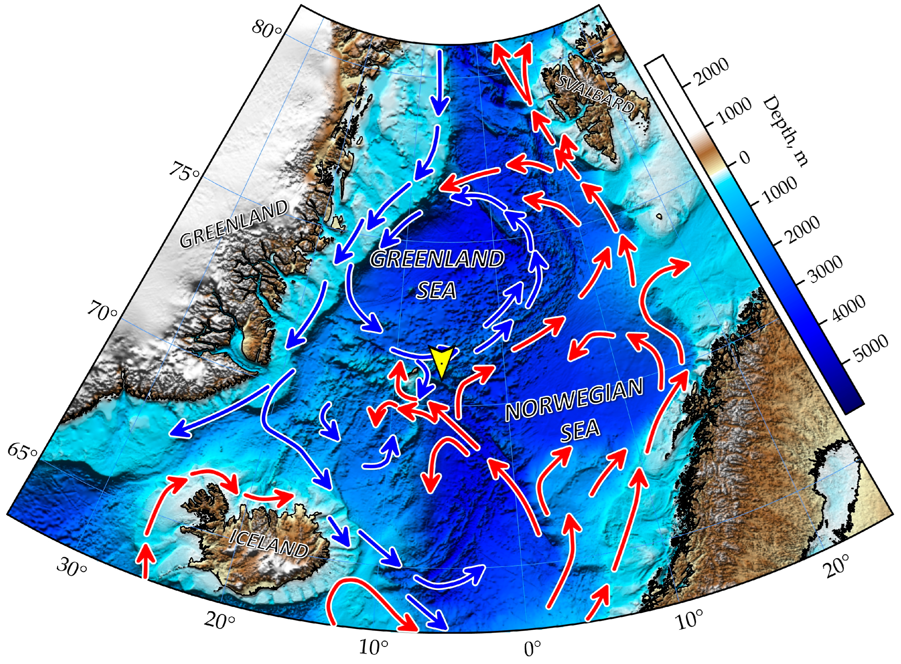
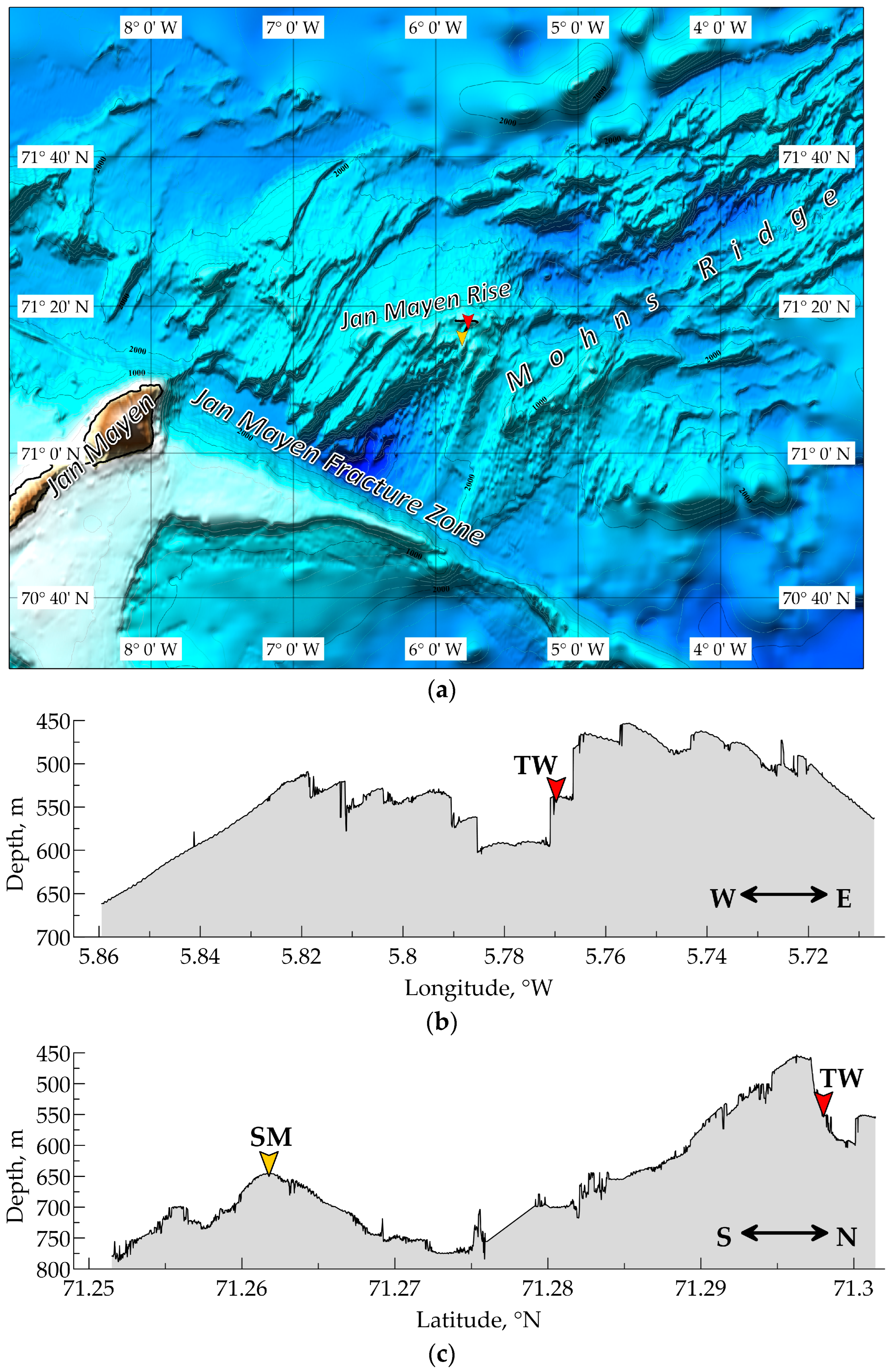
2.1. Study Area

The Mohns Ridge is a segment of the active ultraslow spreading AMOR between 71.2° N and 73.5° N with 1.6 cm/yr full spreading rate [43]. The southernmost segment of the Mohns Ridge is affected by the Iceland and Jan Mayen hotspots and is characterized by anomalously high magmatic activity and shallow water depths (700–550 m) compared to other sections of the ridge [37,44,45,46]. The characteristic structural elements of the Mohns Ridge are AVRs, which are confined to the rift valley [47,48,49,50]. Rift/volcanic structures with hydrothermal activity, such as the JMVFs, may occur within the AVR creating hydroacoustic anomalies above these fields due to gas/fluid release [37]. The Jan Mayen AVR at 71°18′ N is the largest and is located near the Jan Mayen hotspot, which is one of the most active areas of submarine neo-volcanism in the ocean. Its elevation above the rift valley floor is 2100 m. The morphology of the Jan Mayen AVR is very different from that of the other AVRs in the Mohns Ridge. It is also separated from the Jan Mayen Rise by the Jan Mayen Fracture Zone that runs in a northwest to southeast direction (Figure 1 and Figure 2). From the northeast, the Jan Mayen AVR is also bounded by a transform fault. The structure of AVR is complicated by a series of faults and vertical displacements of the dumping type. There are three active vent fields and an inactive one has been discovered and studied at the Jan Mayen AVR summit [37]. Active hydrothermal vent fields include Troll Wall (TW) at 71°18′ N, 5°46′ W and Soria Moria (SM) at 71°15′ N, 5°49′ W) discovered in 2005, and Perl and Bruce explored more recently in 2013; inactive vents include Gallionella Garden [5,37,38].

The bottom-tethered moorings were deployed at TW and SM hydrothermal vent fields (Figure 2), referred to as “TW mooring” and “SM mooring”. The TW vent field is located at a depth of 550 m. It is confined to the fault bounding the eastern wall of the rift valley, which transects the large central volcano Frøya [37]. There are at least 10 major hydrothermal vents associated with several 5–10 m high white smoker chimneys within the TW vent field. Maximum fluid temperature was measured at 270 °C [36,37].

The SM vent field is located 4.3 km to the south of the TW at a depth of 700 m, and is confined to the top of one of the small rifts [37]. The ridges extend in a quasi-meridional direction and are bounded to the east by the northeast-trending rift mountains. The height of the ridges does not exceed 110 m and their width is 250–300 m. At the SM vent field, the maximum vent fluid temperature reaches the same values as at the TW. However, hydrothermal fluids are emitted from two very different types of chimneys. White smoker fluids emerge turbulently from numerous sulfide chimneys up to 8 to 9 m in height, while lower temperature clear fluids escape from irregular constructions made of barite, silica, and minor amounts of pyrite, sphalerite, and galena [36,37].

The hydrography of the study area is described in detail in [41,42]. It is influenced by colder and less salty Arctic-derived waters flowing from the east coast of Greenland as the Jan Mayen Current, and warmer and saltier Atlantic-derived waters supply from the Norwegian Basin as a branch of the Norwegian Atlantic Current (the northern limb of the Gulf Stream system).

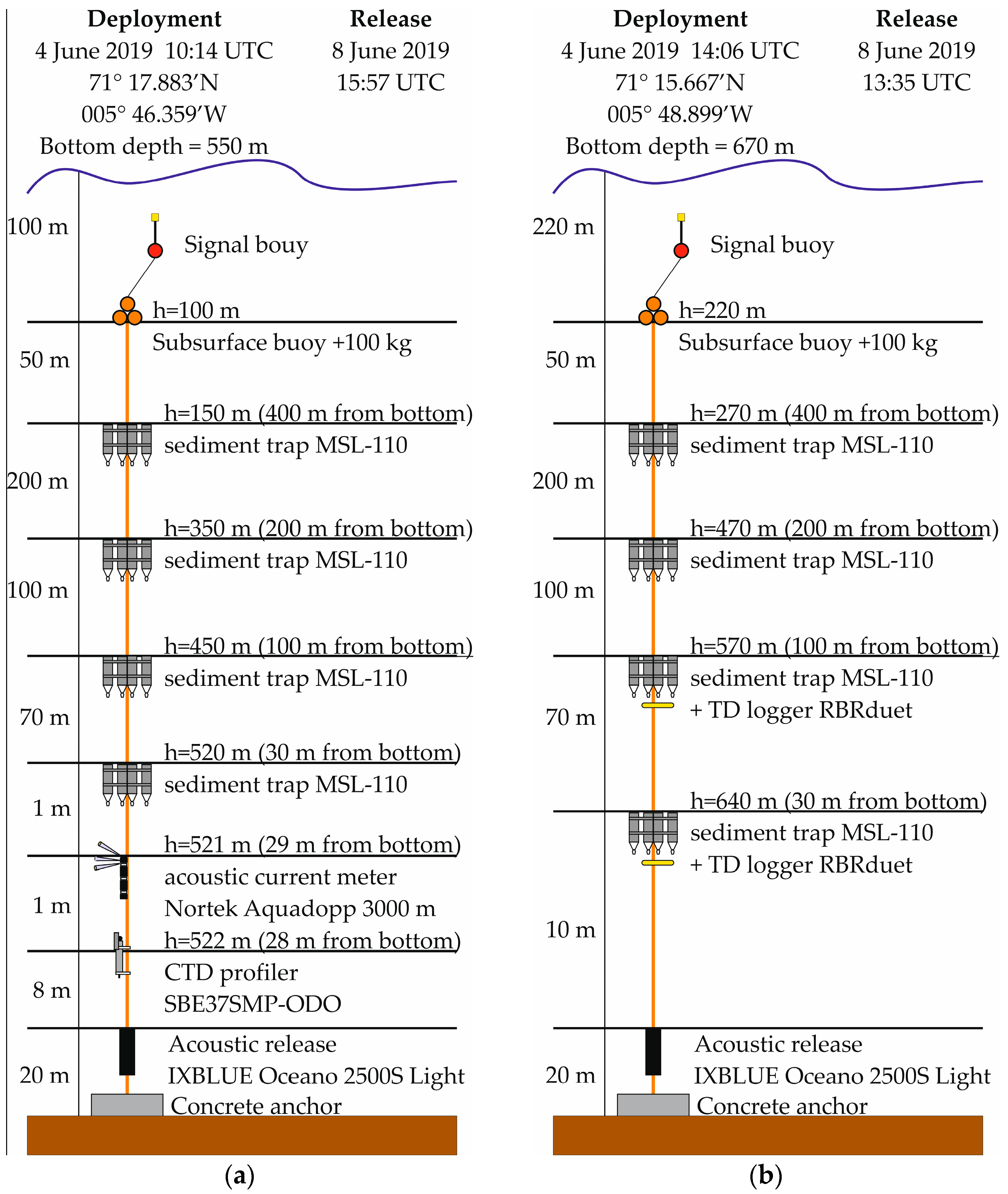
2.2. Field Observations and Sample Collection

Two short-term mooring systems with sediment traps were deployed and recovered during the 75th cruise of the RV Akademik Mstislav Keldysh in June 2019 [51]. The deployment design consisted of a suite of measurement tools operating at different depths (Figure 3). Cylindrical sediment traps MSL-110 (IORAS, Moscow, Russia) [52] were deployed at four nominal depths of 30, 100, 200, and 400 m above the seafloor according to the locations of neutral buoyancy plumes reported in [53]. The distance between traps and vent sources did not exceed 30 m. Autonomous platforms provided continuous sampling with periods of 101.7 and 95.5 h at the TW and SM vent sites, respectively. Trap locations, depths, duration, sinking particle fluxes, and water depth of each deployment are listed in

Table 1. Location of two moorings and particle fluxes at the JMVFs.

Coordinates, Bottom Depth, Duration Time	Actual Trap Depth, m	Flux, mg/m2/day										Content, %
		Total	Si	Al	POC	PIC	CaCO3	LM	bSiO2	Chl-a		Si	Al	POC	PIC	CaCO3	LM	bSiO2
Troll Wall
71°17.883′ N 05°46.359′ W 550 m 101.7 h	150	279.6	29.8	2.15	157.1	2.56	21.36	26.4	52.6	0.291		10.6	0.77	56.2	0.92	7.6	9.4	18.8
	350	100.5	14.5	1.31	43.8	1.08	9.00	16.0	24.3	0.134		14.4	1.3	43.6	1.08	9.0	16.0	24.2
	450	85.6	12.2	1.20	29.9	1.32	11.00	14.7	20.0	0.166		14.3	1.4	34.9	1.54	12.9	17.2	23.4
	520	103.6	14.2	1.26	48.0	2.25	18.73	15.5	23.9	0.260		13.7	1.22	46.3	2.17	18.1	15.0	23.1
Soria Moria
71°15.677′ N 05°48.899′ W 670 m 95.5 h	270	130.3	20.8	1.36	53.8	3.23	26.95	16.6	37.5	0.108		15.9	1.04	41.3	2.48	20.7	12.8	28.7
	470	97.5	12.9	1.11				13.6	21.9	0.193		13.2	1.14				14.0	22.5
	570	90.2	13.6	1.61				19.7	20.8	0.156		15.1	1.78				21.8	23.1
	640	103.9	14.6	1.43				17.6	23.9	0.094		14.1	1.38				16.9	23.0

.

Quadrupled cylindrical MSL-110 sediment traps (IORAS, Moscow, Russia) with the inner diameter of each tube of 110 mm, i.e., four tubes per layer with a total collection area of 0.038 m², were deployed at each trap depth of the moorings. The ratio between diameter and collecting tube length is 1:6 [52]. The MSL-110 sediment trap design has previously been successfully utilized in the study of sinking particle fluxes in the Arctic Seas and the subpolar North Atlantic [54,55]. The collecting cups of the traps were filled with 0.45 µm filtered intermediate seawater made up to a salinity of 40 psu with NaCl. No poison was applied to the collecting cups during deployment.

Nortek Aquadopp Current Meter (Nortek AS, Rud, Norway) and SBE37SMP-ODO CTD profiler (Sea-Bird Electronics, Inc., Bellevue, WA, USA) equipped with an SBE63 Optical Dissolved Oxygen Sensor (Sea-Bird Electronics, Inc., Bellevue, WA, USA) were deployed at 1 m below the 520 m trap depth at the TW mooring to measure relative water motions and hydrographic parameters. RBRduet T.D loggers (RBR Ltd., Ottawa, ON, Canada) were deployed immediately below the 570 m and 640 m trap depths at the SM mooring to measure hydrographic data.

In order to document the water column properties, CTD profiling with Seabird SBE911plus (Sea-Bird Electronics, Inc., Bellevue, WA, USA) was carried out at two stations before deployment and after the recovery of the moorings. To assess the concentration of suspended particulate matter (SPM), particulate organic carbon (POC), and chlorophyll a (Chl-a), water samples were collected using Niskin bottles (OceanTest Equipment, Fort Lauderdale, FL, USA) equipped sampling system SBE 32 (Sea-Bird Electronics, Inc., Bellevue, WA, USA). Samples were collected from the subsurface, chlorophyll fluorescence maximum, and near-bottom layers according to CTD profiles, and were then divided into subsamples to determine total SPM, POC, and Chl-a concentrations.

2.3. Processing and Analysis of Samples

The material collected by the traps, as well as water samples from Niskin bottles, were filtered under vacuum through pre-weighed nuclear pore membrane filters with a diameter of 47 mm and a pore size of 0.45 µm. Salts were eliminated by rinsing the filtered samples several times with MilliQ water at the end of filtration. The filters were dried at 50 °C, and then weighed using a Sartorius analytical electronic balance with an accuracy of ±0.01 mg. The deposited mass was calculated from the difference between the final and initial weights of the filter. The total particle flux was obtained by dividing the deposited mass by the sediment trap collection area and collection time. The mass concentration of the SPM was obtained by dividing the deposited mass by the volume of the filtered seawater.

Subsamples for the determination of total particulate carbon (TC), particulate organic carbon (POC), and particulate inorganic carbon (PIC) and chlorophyll a (Chl-a) were filtered under a low vacuum onto Whatman GF/F glass microfiber filters of 47 mm diameter and a pore size of 0.7 µm precombusted at 500 °C for 4 h.

Chl-a concentrations were determined fluorometrically according to [56,57]. Whatman GF/F glass microfibre filters with trapped material were extracted in 90% acetone (at 2 °C in the dark for 24 h). The fluorescence of the extracts was measured with a Trilogy laboratory fluorometer version 1.1 (Turner Designs, San Jose, CA, USA) before and after acidification with 1 N HCl. The accuracy of determination was ±0.02 mg/m³.

Total particulate Si and Al were determined using the photometric method with a UNICO 1201 device (United Products & Instruments, Inc., Dayton, NJ, USA) according to [58]. The sample was fused previously in a muffle furnace (at a temperature of 950 °C for 4 h) with a mixture of Na₂CO₃ and Na₂B₄O₇ and the addition of KNO₃. The fusion was dissolved in 3M HCl. The measurement of dissolved silicon concentration involves the molybdate-blue spectrophotometry of the extract at a wavelength of 815 nm. The colorimetric determination of Al is based on the ability of Al to form a red-colored complex with aluminon. Starch is used to preserve the red-colored complex as a colloidal suspension. The optical density of the solution is measured spectrophotometrically at a wavelength of 525 nm. The standard reference matter (SRM) of ocean sediments (OOPE-101 and OOPE-401, Research Institute of Applied Physics (RIAP), Irkutsk State University, Irkutsk, Russia) was used to assess the quality of the analysis. The discrepancies with the SRM passport values of the contents of the measured elements in SRM were 2–5%. The content of lithogenic matter (LM) was calculated by multiplying the Al by a factor of 12.27 based on the average aluminum content in the upper continental crust (UCC) [59]. The silicon content exceeding the lithogenic content estimated by the Si/Al ratio in the UCC [59] was considered as exSi. The Si enrichment of SPM relative to lithogenic matter is usually explained by the presence of biogenic amorphous silica (bSiO₂) [60].

Particulate total carbon (PTC) and PIC were measured with a Shimadzu TOC-L analyzer with an SSM-5000A module (Shimadzu Corporation, Tokyo, Japan). IC was measured directly by coulometry, which is the measurement of CO₂ following the closed-system conversion of IC to CO₂ upon the addition of phosphoric acid [61]. POC was determined by the difference between PTC and PIC. The analytical accuracy was 1.0 wt.%. From the PIC content, the particulate calcium carbonate CaCO₃ was calculated by multiplying 8.33 (according to stoichiometric coefficients and atomic weights).

The elemental analysis of sinking material was carried out by inductively coupled plasma mass spectrometry (ICP-MS) using the Agilent 7500a quadrupole instrument (Agilent Technologies, Inc., Santa Clara, CA, USA). Filters with the weighed matter were placed in Teflon (Savillex™, Eden Prairie, MN, USA) vials; filled with a mixture of nitric, hydrofluoric, and hydrogen peroxide ultrapure concentrated acids in the proportion of 10:2:3; placed in an ultrasonic bath for 90 min at a temperature of 70 °C; and then were kept overnight [62]. After that, the filters were removed from the vials and washed with a small amount of 0.1 N nitric acid. Then, with the addition of hydrochloric acid, the samples were evaporated three times on a hotplate. After the last evaporation, the samples were brought to a volume of 35 mL with deionized water. A multi-element standard curve containing 10 ppb of indium was used to calculate trace element concentrations after the subtraction of the instrument blank. Digest blanks were subtracted from the sample and filter blanks were adjusted for a blank derived from the digestion acids and Teflon vials. The overall analytical precision was 5–10% based on five replicate analyses of a single sample digest solution.

To assess the sources of material input, elemental concentrations were normalized to the average crustal composition, and enrichment factors (EFs) relative to the average UCC composition [59] were calculated using the following equation:

EF = (El/Al)_sample/(El/Al)_UCC,

(1)

where (El/Al) is the ratio of element to Al content in the sample or UCC. EF values close to 1 (less than 3) indicate a predominantly lithogenic origin of the material, whereas EF values greater than 3 indicate an additional source (e.g., biogenic accumulation, chemical precipitation, ore minerals admixture, etc.).

Based on the Fe and Al content data, the excess iron Fe_ex content was calculated as follows:

Fe_ex = Fe_measured − Al_measured × (Fe/Al)_UCC,

(2)

where Fe_measured and Al_measured are the measured Fe and Al contents in the sample, (Fe/Al)_UCC is the ratio of these elements in the Earth’s crust.

The cerium and europium anomalies (Ce_an and Eu_an respectively) in the samples were calculated using the following equations [63]:

Ce_an = Ceⁿ · 2/(Laⁿ + Prⁿ),

(3)

Eu_an = Euⁿ · 2/(Smⁿ + Gdⁿ),

(4)

where Elⁿ is the REE content in the sample normalized to the content in NASC shale [64].

The ratio of light to heavy REEs was calculated using the formula:

LREE/HREE = (La^N + 2 × Pr^N + Nd^N)/(Er^N + Tm^N + Yb^N + Lu^N),

(5)

This formula avoids biases associated with anomalous accumulation of REEs of variable valency [65]. All the REEs have been normalized to the NASC shale composition.

The micromorphology was studied with a VEGA-3sem TESCAN scanning electron microscope (Brno, Czech Republic). For observation in the secondary electron (SE) mode, the samples were coated with a 3 to 5 nm thick gold layer. The chemical composition was studied on polished gold-coated samples (BSE mode) via energy-dispersive X-ray spectroscopy with an Oxford INCA Energy 350 microanalyzer (Oxford Instruments, Abingdon, UK) and a VEGA-3sem TESCAN scanning electron microscope (Brno, Czech Republic). The SEM-EDS spectra were recorded at an accelerating voltage of 20 kV and electron beam diameter < 1 μm. The spectra were calibrated and quantitatively optimized along the Si Ka 1.73982 kV line. The element concentrations in sulfides were determined taking into account corrections for the absorption and scattering of X-rays using the INCA program, v. 4.15. The element detection limit was 0.2 wt.%.

2.4. Satellite Research

To study the bio-optical characteristics of the sea surface water, MODIS-Aqua ocean color scanner data were retrieved from the NOAA website (https://oceancolor.gsfc.nasa.gov/, accessed on 28 April 2022). The 8-day composite Level 3 Mapped Chlorophyll Data at moorings locations with a spatial resolution of 4 × 4 km was averaged. Satellite data were processed using the SeaDAS 8.2.0 software (https://seadas.gsfc.nasa.gov/, accessed on 4 April 2022).

3. Results

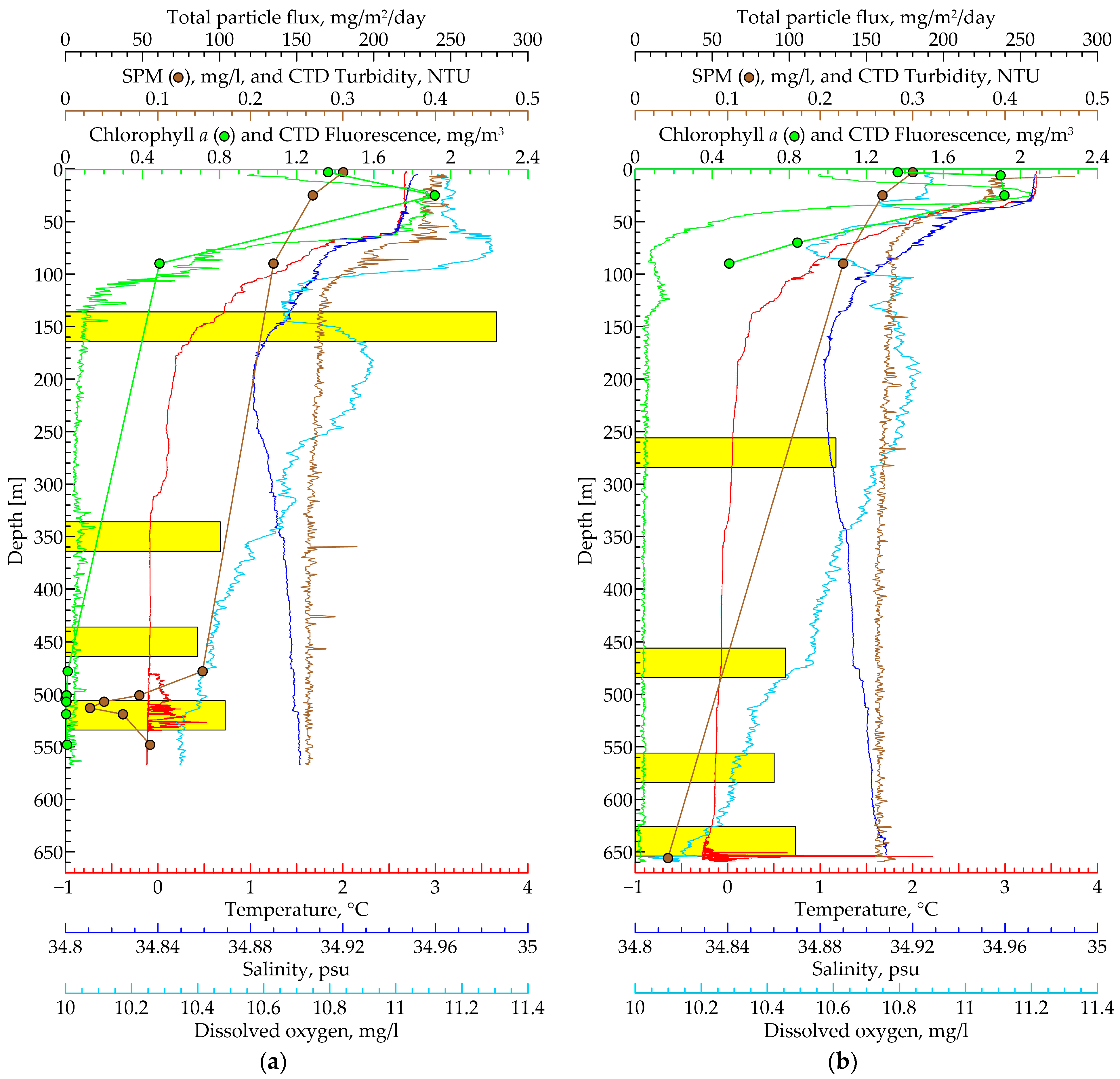
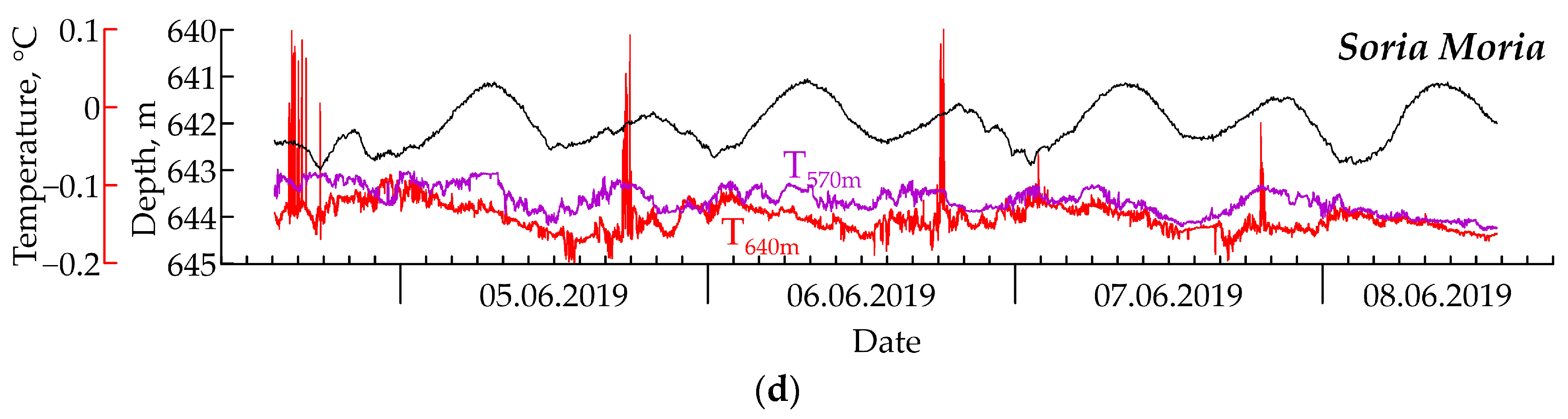
3.1. Environmental Conditions at the Mooring Sites

The temperature, salinity, and turbidity profiles were obtained before the deployment and after the retrieval of the moorings (see Figure 4). Most of the water column (from the bottom to ~140 m) was occupied by cold Arctic intermediate water (temperature −0.26–0.3 °C, salinity 34.88–34.91 psu), and only the upper quasi-homogeneous layer 0–60 m warmed to 2–3 °C (Figure 4). The background temperature in the deep water layers (up to 100 m from the bottom) varied from −0.13 °C to 0.12 °C and from −0.26 °C to 0.13 °C at the TW vent field and the SM vent field, respectively. CTD measurements during the deployment and retrieval of moorings revealed positive temperature anomalies near the bottom with an amplitude of 0.64 °C in the TW and 2.49 °C in the SM (Figure 4). Positive temperature anomalies were recorded in the 40–90 m layer from the bottom in the vicinity of the TW field and were maximally confined to the bottom (0–15 m) in the SM field.

Acoustic current meter data obtained from the TW mooring (Figure 5) revealed fluctuations in current velocity ranging from 0.3 to 18.7 cm/s, with an average velocity of 6.1 cm/s. Regular variability in current speed and direction with a semi-diurnal cycle was observed, indicating tidal influence. The accumulated water mass transport (vector sum) during the deployment time of the TW mooring amounted to 8092 m. Based on this value, the average vector velocity of lateral particle transport is calculated to be 2.2 cm/s. At the TW mooring, several pronounced short-term above-zero temperature anomalies with amplitudes of up to 0.86 °C were recorded in the near-bottom layer. The minima of the dissolved oxygen concentrations and the maxima of the sound backscattering by particles, obtained with the acoustic Doppler current meter, are associated with the temperature anomalies.

T.D loggers in the near-bottom layer of the SM vent field also recorded above-zero temperature anomalies, but with a much smaller amplitude (~0.25 °C). The temperature anomalies were observed only once a day and were related to the tidal phase during the day (Figure 5). No similar temperature anomalies were detected 70 m higher, at the next level from the bottom (570 m).

In the SM vent field, a cold layer with a temperature of −0.26 °C, which is 0.13 °C below the background value, was observed near the bottom by CTD profiling prior to mooring deployment. The layer was approximately 50 m thick. The CTD profiling after mooring recovery did not detect this layer. Fluctuations in the water temperature of the same amplitude (up to 0.13 °C) were also recorded by the sub-bottom T.D loggers. The period of variation was 1 day. This is characteristic of the diurnal component of the tides.

3.2. Suspended Particulate Matter and Chlorophyll a

SPM concentrations in the water column prior to mooring deployment ranged from relatively high values of 0.23–0.30 mg/L in the upper (0–90 m) layer to a low value of 0.03–0.09 mg/L in deeper waters (see Figure 4). The upper mixed layer (0–25 m) was characterized by high Chl-a concentrations of 1.36–1.92 mg/m³ at the mooring sites and up to 5.4 mg/m³ in the adjacent area (30 miles to the west in the Arctic Front). The Chl-a concentrations exhibit a subsurface maxima at the depth of 25–35 m. With increasing depth to 100 m, the concentrations of Chl-a gradually decreased to 0.2 mg/m³, and below 100 m, it reached a minimum value (≤0.01 mg/m³).

3.3. Mass Fluxes and Major Element Composition

3.3.1. Total Particle Fluxes

The maximum vertical particle flux (279.6 mg/m²/day) occurs in the 150 m subsurface layer at the TW vent field (Figure 4, Table 1). Deeper down, from 270 m to the bottom, fluxes ranged from 85 to 130 mg/m²/day. Minimum fluxes (85–97 mg/m²/day) were recorded in the 450–570 m intermediate layer at both sites. Particle fluxes in the near-bottom layer (30 m from the bottom) were found to increase to 103.6 mg/m²/day and 103.9 mg/m²/day at the TW vent field and SM vent field, respectively. This may be an indication of the hydrothermal supply. The study of the distribution of SPM, both by membrane filtration and by turbidity sensor at the CTD profiler, did not reveal the presence of a pronounced nepheloid layer near the bottom of the study area. This was also found in the work of M.D. Kravchishina et al. [39].

3.3.2. Major Phase Composition of Particles Including POC, PIC (CaCO₃), bSiO₂, and Lithogenic Matter

The sedimentary matter is dominated by biogenic components including CaCO₃ + POC + bSiO₂. These components reached ~99% in the upper layer (150 m) of the water column above the TW vent field (Table 1). The POC ranges from 35% to 56%. The maximum is found in the subsurface layers. A high content of bSiO₂ (18.8–28.7%) was observed almost constantly throughout the water column, and maximum fluxes of 52.6 mg/m²/day and 37.5 mg/m²/day localized in the 150 m (TW mooring) and 270 m (SM mooring) subsurface layers, respectively. Subsurface water is also responsible for the maximum CaCO₃ flux. The flux of lithogenic particles increased below the euphotic zone and remains almost constant (13.6–19.7 mg/m²/day) from the layer of 270 m to the bottom at both vent fields, accounting for 12.8–21.8% of the sinking matter.

3.3.3. Electron Microprobe Analysis of Particles

In the studied water column, with the exception of the bottom layers of both fields, biogenic material (diatoms, coccolithophorids, and foraminiferal test fragments) and particles of rock-forming minerals of pelitic and fine silty grain size (feldspars, quartz, augite, andalusite, clay minerals, etc.) prevailed. Hydrothermally derived micron-sized minerals such as sulfides, sulfates, amorphous silica, etc., were abundant in the benthic layers of both vent fields.

Troll Wall

At a depth of 350 m, along with biogenic particles, a significant amount of mineral particles ranging in size from 2 µm to 20 µm were present. Particles finer than 2 µm often form isometric aggregates ≥ 50 µm in size, dominated by aluminosilicate clay particles mixed with algal skeletal fragments (Figure S1a). In addition to clay particles in the aggregates, EDS data revealed many unrounded grains of rock-forming minerals: forsterite, diopside, anorthite, K-feldspar, labrador, pseudorutile and titanomagnetite (Table S1). Deeper down, at a depth of 450 m, clay particles (up to 5 μm), organomineral aggregates (up to 20 μm) and feldspars (15–25 μm) were found along with forsterite and feldspar particles of irregular isometric shape with fresh fractures. An abundance of biogenic detritus and clay particles 5–10 µm in size was also observed in the bottom layer at 520 m. Of the main minerals that form the rock, particles of diopside and augite were found in this layer. The bottom layer contained a large amount of hydrothermally derived minerals:

• Gypsum microcrystallites up to ~140 µm in size formed by free growth were characterized by a columnar habitus with well-formed, flattened, elongated prismatic faces showing dissolution shapes (Figure S1b). The chemical composition of the gypsum was close to the stoichiometric composition and no significant concentrations of isomorphic impurities were found in the gypsum (Table S2).
• Barite aggregates ~120 µm in size have lamellar and tabular habitus (Figure S1c). Flat barite crystals > 10 µm with a crosscutting tabular shape of hexagonal type were identified in the aggregates. The tabular crystals formed well-shaped rosette structures at both vent sites. According to the EDS data (Table S2), the barites demonstrated a minor substitution of barium by strontium and calcium. Barite aggregates formed a stable mineral association with sulfides.
• Iron, copper, and zinc sulfide minerals formed porous as bud-shaped masses with individual spherulites ≤ 0.5 µm in size, often of complex chemical composition with impurities (Figure S1d). Only pyrite formed regular octahedrons and cuboctahedrons up to 3 µm in size.
• Aggregates of non-crystalline Fe-Si oxyhydroxides of separate thin filaments of 0.5–1 µm diameter of isometric, sheaf, and whorl shapes characteristic of the quenching process under conditions of high temperature difference (Figure S1e). Microspheres up to 0.5 µm were embedded in the filaments of the whorls. The EDS data indicated that the SiO₂ content of the aggregates ranged from 27 to 41 wt.% and that they exhibited a significant iron impurity (38–45 wt.%) as well as calcium (Table S3).

Soria Moria

The particle composition at depths of 270–570 m was notably similar to that of the upper and intermediate water layers (150–450 m) of the TW vent field. The prevailing constituents were biogenic matter, clay minerals, and particles of rock-forming minerals with a size of 10–15 µm. These included feldspars, quartz, augite, and andalusite. The latter was frequently characterized by an unrolled surface displaying fresh chipping or cleavage patterns (Figure S1f, Table S4). The particle composition of the 640 m near-bottom layer appears to be similar to that of the 520 m near-bottom layer of the TW field. In addition, biogenic particles and organo-mineral aggregates were also observed to be predominant. Among the mineral particles, clay minerals, single particles of rock-forming minerals, and hydrothermally derived minerals were identified:

• Barite aggregates up to 50 µm in size with a lamellar and tabular habitus (Figure S1g), and minor substitution of barium by strontium (Table S5);
• Sulfide minerals, represented by the well-formed octahedrons of pyrite and sphalerite up to 6 µm (Figure S1h), as well as sulfide phases of complex composition in the form of dendrites and solid masses (Figure S1i);
• Aggregates of noncrystalline Fe-Si oxyhydroxides from individual thin filaments of similar diameter and shape as in the TW field (Figure S1j). EDS data indicates that the content of SiO₂ in aggregates is 32–34%. In addition to iron (34–37 wt.%) and calcium, they also contain a significant admixture of phosphorus (up to 3 wt.%) (Table S6).

No gypsum microcrystallites were identified in the sinking material from the SM field.

3.3.4. Major and Trace Element Composition and REE

The trace element composition of the sinking matter is heterogeneous and exhibits a significant depth-related variability (

Table 2. Elemental composition of the sinking material.

Depth, m	Fe	Al	P	Ti	V	Cr	Mn	Co	Ni	Cu	Zn	Ga	As	Rb	Sr	Zr	Nb	Mo	Cd	Cs	Ba	Hf	Ta	Tl	Pb	Th	U
	%	%	%	ppm
Troll Wall
150	0.50	0.77	0.37	785	21.4	16.7	347	2.87	20.35	41.1	1147	1.85	6.36	4.98	486	14.84	4.16	1.081	2.34	0.106	330.1	0.345	0.540	0.013	31.9	0.418	2.048
350	0.88	1.30	0.32	1685	36.1	34.4	854	5.42	43.05	269	1149	1.78	11.08	6.66	552	27.97	8.28	2.482	1.12	0.008	332.3	0.492	0.877	ND	52.2	0.416	1.192
450	1.30	1.40	0.23	1619	49.8	44.9	1472	7.17	42.34	256	1382	3.60	44.59	11.30	521	33.98	8.34	3.182	1.83	1.265	1187	0.558	0.886	0.143	81.5	0.824	1.320
520	1.60	1.22	0.2	1494	49.0	31.4	873	6.76	39.40	575	3170	3.39	12.41	8.34	2553	25.31	7.30	4.276	17.32	0.074	4921	0.480	0.802	0.535	100.3	0.514	1.350
Soria Moria
270	0.76	1.04	0.25	1361	29.2	22.5	556	4.19	27.19	116.1	1223	2.05	12.35	6.15	827.9	24.92	6.82	1.719	0.88	0.127	531	0.460	0.616	0.013	49.82	0.431	1.075
470	0.84	1.14	0.26	1536	37.3	33.1	1103	5.44	35.37	138.2	1222	2.55	13.11	7.40	445.7	26.78	7.51	1.798	3.74	0.124	558	0.472	0.721	0.031	50.83	0.534	1.012
570	1.16	1.78	0.21	1960	47.0	33.5	745	6.38	48.27	208.1	1058	2.90	6.83	8.94	504.2	34.71	9.69	1.763	0.61	0.106	612	0.794	1.006	0.017	74.78	0.652	0.978
640	1.09	1.38	0.19	1764	45.6	57.9	698	6.76	42.42	515.6	11,740	3.55	18.82	8.25	2857	28.61	9.44	6.864	18.37	0.111	12,435	0.574	1.030	4.843	163.17	0.599	1.037

). In both fields, the settling matter has similar elemental composition characteristics. The concentration of sulfide-forming elements, including Cu, Zn, Pb, Fe, and Mo, and other hydrothermally derived elements, such as Ba, Sr, Cd, Tl, and Eu, increases with depth and reaches a maximum value at a distance of 30 m from the bottom (depths of 520 and 640 m) (Table 2). With regard to other elements (both hydrothermally derived and rock-forming), the maximum content at 100 m from the bottom (depths of 450 and 570 m) is characteristic for Mn, V, Cr, Co, Ga, As, Rb, Y, Zr, Cs, Al, Hf, Th, as well as for most REEs (

Table 3. Rare earth element content in the sinking material.

Depth, m	Sc	Y	La	Ce	Pr	Nd	Sm	Eu	Gd	Tb	Dy	Ho	Er	Tm	Yb	Lu
	ppm
Troll Wall
150	1.9	2.9	4.3	7.9	1.02	3.9	0.68	0.22	0.74	0.09	0.58	0.11	0.32	0.03	0.27	0.04
350	2.3	3.7	6.1	11.5	1.50	5.8	1.20	0.33	1.12	0.13	0.87	0.16	0.54	0.05	0.37	0.07
450	3.6	4.9	12.8	28.3	2.07	8.9	1.79	0.52	1.24	0.19	1.22	0.19	1.42	0.06	0.47	0.08
520	3.5	3.8	6.9	13.0	1.45	6.1	1.38	0.46	1.08	0.14	0.86	0.13	0.39	0.05	0.27	0.06
Soria Moria
270	2.4	3.5	5.9	10.7	1.38	6.1	0.98	0.27	1.07	0.13	0.79	0.13	0.46	0.03	0.31	0.05
470	2.8	4.0	7.0	13.9	1.87	7.3	1.22	0.34	1.07	0.13	0.84	0.12	0.58	0.05	0.41	0.05
570	3.0	4.8	9.4	17.2	1.93	8.0	1.48	0.39	1.28	0.18	0.99	0.18	0.60	0.05	0.44	0.05
640	2.6	4.2	7.6	14.9	1.83	6.7	1.36	0.40	1.34	0.13	1.01	0.16	0.51	0.06	0.44	0.07

). The remaining elements (Si, P, Ti, Ni, Nb, Ta, U, and Gd) do not exhibit a discernible correlation with depth. However, it can be observed that their content generally increases in the deep water layer compared to the upper layer (0–150 m).

The content of Al ranges from 0.77 to 1.78 wt.%, with an average of 1.25 wt.%. The lowest content of rock-forming elements, including Al, Ti, Zr, and Hf, as well as Nb, Ta, Ni, and Y, which are components of the rock-forming and accessory minerals of igneous rocks, was identified in the sinking matter of the subsurface 150 m layer. The greatest values of their content are observed at a depth of 100–200 m above the bottom, corresponding to depths of 450–350 m in the TW field and 570–470 m in the SM field (Table 2). A robust linear relationship was observed among the items within this group, where the coefficient of determination (R²) ranged from 0.78 to 0.93.

In order to ascertain the potential for a non-detrital origin for the Si concentration in the trapped matter, a plot of Si against Al was constructed (Figure 6a). A correlation coefficient of 0.60 has been determined for the pairwise relationship between Si and Al in the samples. Si normalized to Al varies from 8.5 to 15.3 while the average crustal ratio (Si/Al)_UCC = 3.83 [59], indicating the input of amorphous biogenic silica—bSiO₂. Concurrently, the enrichment factor (EF) for Si reaches 3.6–4.0 in the upper layers of the water column, predominantly as a consequence of silicon-containing phytoplankton. The Si/Al ratio in the bottom sediments varied from 1.3 to 3.9 [66].

The majority of elements exhibit EF values that are less than three. The following elements have been identified as having an additional source other than rock-forming: Cu, Zn, Tl, Co, V, Ga, Cd, Sr, Mo, Pb, Eu, and Ba (Figure 7). The values of the EF for Cu, Zn, Sr, Ba, Mo, Cd, and Eu significantly increased at both fields in the lowermost depths. The SM field demonstrates a more than 10-fold increase in the values of EF elements (Cu, Zn, Sr, Ba, Mo, and Cd) when compared to the overlying layer. This indicates an increase in the proportion of hydrothermally derived sulfides and sulfates in the bottom layer.

The Ba content reaches 0.4 and 1.2 wt.% in the bottom layer of the TW and SM vent fields, respectively. As the depth decreases, the Ba content in both fields declines and reaches values up to 0.1–0.06 wt.%. Sinking material throughout the water column is enriched in Ba relative to the average crustal ratio ((Ba/Al)_UCC = 0.008): EF varies from 3 to 11 in the upper and deep water layers and reaches 50–113 near the bottom. Ba exhibits a reliable correlation with a high pair correlation coefficient (R = 0.76–0.98) in the presence of certain elements: Zn, Pb, Mo, Tl, Eu, Sr, Cu, and Cr (in descending order of R). The majority of these elements exhibit chalcophilic (Zn, Pb, Mo, Tl, and Cu) or siderophilic (Cr) properties.

The most pronounced enrichment of sulfide-forming elements, including Fe, Cu and Zn, relative to the average crustal ratio (Fe(Cu, Zn)/Al)_UCC, is observed in the material trapped near the bottom (Figure 7). With regard to Fe, the highest EF is observed in the near-the-bottom layer at the TW vent field. For Cu, a significant enrichment of sinking material is observed throughout the deep water column of both fields. However, the maximum EF value is also reached in the benthic layer of the TW vent field. In contrast, the greatest enrichment of Zn is observed in the bottom layer of the SM vent field, where its content reaches 1.2 wt.%, which is four times higher than its concentration in the same layer of the TW field (Table 2). Fe shows the strongest correlations with Co, V, Ga, and Cu, while Cu correlates most with Cd, Sr, Mo, Pb, Eu, Ba, and Zn. Zn, in turn, shows the strongest correlations with Tl, Ba, Pb, Mo, Eu, Sr, Cr and Cu. The concentration of Cu and Pb in the near-the-bottom layer is about twice that of the overlying water column, while the concentration of Sr is about five times higher. The concentration of Pb is about two-fold and that of Tl is nine-fold higher in the sinking material at the bottom of the SM vent field than at the bottom of the TW field. With regard to Cd, the highest degree of enrichment (EF 10 times higher than the average crustal ratio (Cd/Al)_UCC) was observed in the benthic layer at the TW field.

The particulate Mn concentration in the water column is characterized by an enrichment of trapped matter, with the highest concentrations observed at a depth of 450–470 m at both vent fields. The concentration of Mn in the deep water column is slightly higher in the TW vent field than in the SM vent field. Mn shows robust correlations with Cs, As, and Rb, as well as with some light rare earth elements (LREEs), including Ce, Sm, La and Nd, and Th. The highest concentration of labile elements, including As and Cs, and Rb, is observed at a depth of 100 m above the bottom (layer of 450 m) at the TW vent field (Table 3).

The concentration of LREEs in the sinking material shows a range of values, varying from 18 to 54 ppm at the TW vent field and from 25 to 38 ppm at the SM vent field. The concentration of LREEs reached its maximum value at a depth of 100 m above the bottom at the TW vent field. At the same time, the shale-normalized REE patterns of sinking material show both slight negative Ce anomalies, and positive Eu anomalies (Figure 8,

Table 4. Different calculated ratios for REE.

Location/ Depth, m	Feex	Mn	ΣREE	Cean	Euan	(La/Yb)N	(La/Sm)N	(LREE/ HREE)N
	%		ppm
Troll Wall
150	0.13	0.03	20.3	0.82	1.35	1.55	1.12	1.52
350	0.25	0.09	29.8	0.83	1.23	1.59	0.91	1.44
450	0.63	0.15	59.3	1.17	1.50	2.66	1.27	1.84
520	1.01	0.09	32.3	0.89	1.64	2.45	0.89	1.81
Soria Moria
270	0.26	0.06	28.3	0.82	1.14	1.85	1.08	1.59
470	0.29	0.11	34.8	0.83	1.30	1.64	1.03	1.80
570	0.30	0.07	42.2	0.87	1.23	2.06	1.13	1.95
640	0.43	0.07	36.5	0.87	1.29	1.68	1.00	1.64
Mohns Ridge basalts [68]
		0.09–0.12	25.4–69.3	0.87–0.89	1.36–1.50	0.11–0.47	0.20–0.60	0.20–0.53
Jan Mayen alkaline basalts [68]
		0.12–0.16	131–209	0.90–0.91	1.38–1.50	1.19–2.49	0.77–1.14	1.21–2.35
Atlantic hydrothermal vent fields sulfides [69]
			75–451	0.50–0.87	0.6–21	0.21–6.40	0.39–7.32	0.44–1.84
TAG vent field anhydrites [70]
			2930–21,290	0.85–0.88	2.25–13.2	0.97–2.68	0.17–0.47	4.00–6.59

), as well as a depletion of matter with REEs compared to NASC. The greatest depletion of REEs was observed at a depth of 150 m in the TW field, where the biogenic content reached its highest value.

3.3.5. Trace Element Fluxes

A calculation was performed to determine the vertical fluxes of a number of sulfide-forming elements (Zn, Cu, Mo, etc.), as well as those of Ba, Sr, Cd, etc. (

Table 5. Vertical fluxes of hydrothermally derived elements at JMVFs compared to published data for other submarine vent fields.

Depth, m	Fluid T, °C	Bottom Depth, m	Total Flux	Fe	P	Cu	Zn	Sr	Mo	Cd	Ba	Tl	Pb	Mn	Rb	Cs	V	Cr	Co	Ni	Ga	As	La	Eu
			mg/m2/day		µg/m2/Day
	Troll Wall
150			279.6	1.40	1034.5	11.49	320.73	136.12	0.302	0.653	92.3	0.0037	8.93	97.1	1.392	0.0297	5.99	4.66	0.801	5.69	0.518	1.778	1.203	0.0495
350			100.5	0.88	321.6	27.06	115.48	55.49	0.249	0.112	33.4	ND	5.25	85.9	0.670	0.0008	3.63	3.46	0.545	4.33	0.179	1.113	0.618	0.0264
450			85.6	1.11	196.9	21.95	118.32	44.65	0.272	0.156	101.6	0.0123	6.98	126.0	0.967	0.1083	4.27	3.84	0.614	3.62	0.308	3.816	1.096	0.0356
520	270 * 119–276 **	550	103.6	1.66	207.3	59.6	328.5	264.6	0.443	1.795	510	0.0555	10.40	90.5	0.865	0.0077	5.08	3.25	0.700	4.08	0.351	1.286	0.715	0.0381
****		520/450	1.2	1.5	1.05	2.7	2.8	5.9	1.6	11.5	5.0	4.5	1.5	0.7	0.9	0.1	1.19	0.85	1.14	1.13	1.14	0.34	0.65	0.0279
	Soria Moria
270			130.3	0.99	325.7	15.12	159.44	107.87	0.224	0.115	69.2	0.0017	6.49	72.5	0.802	0.0165	3.80	2.93	0.546	3.54	0.267	1.609	0.771	0.0265
470			97.5	0.82	253.6	13.48	119.26	43.48	0.175	0.365	54.5	0.0031	4.96	107.7	0.722	0.0121	3.64	3.23	0.531	3.45	0.249	1.279	0.683	0.0280
570			90.2	1.05	189.4	18.76	95.47	45.47	0.159	0.055	55.2	0.0015	6.74	67.2	0.806	0.0095	4.24	3.02	0.576	4.35	0.261	0.616	0.850	0.0333
640	270 *	670	103.9	1.13	197.5	53.6	1220.3	297.0	0.713	1.910	1293	0.5034	16.96	72.6	0.857	0.0115	4.74	6.02	0.703	4.41	0.369	1.956	0.789	0.0495
****		640/570	1.2	1.1	1.04	2.9	12.8	6.5	4.5	34.6	23.4	330.6	2.5	1.1	1.1	1.2	1.12	2.00	1.22	1.01	1.41	3.18	0.93	2.6
	Endeavor Ridge, Juan de Fuca Ridge, N–E Pacific [71]
2050–2700	124–283	2200	754	119.6		9096	7808	1370			4137			196.1
	Totem, 13° N East Pacific Rise [31]
2600	380	2600	11,589	2318	849	8685	10,658						16,219	1726			290
	13° N East Pacific Rise [29]
2600	380	2600	667	103		2535	13,000							5336
	Menez-Gwen, 37°50′ N Mid-Atlantic Ridge [72]
847–871	265–284 ***	850	640	8.3		3200					10,880
	Lucky Strike, 37°50′ N Mid-Atlantic Ridge [15]
1618–1730	152–333 ***	1700	264	16.3		2455					8422
	Rainbow, 36°14′ N Mid-Atlantic Ridge [13]
2270–2320	360–365 ***	2320	6900	496.8		345,000					17,250
	Broken Spur, 29°10′ N Mid-Atlantic Ridge [28]
~3000	356–364 ***	3090	1800	668		12,600	12,600				660
	TAG, 26°08′ N Mid-Atlantic Ridge [73]
3670	270–363 ***	3650	5200	1820		52,000	44,000				4732

* [37]; ** [39]; *** after [30]; **** excess factor (bottom (“hydrothermal”) flux/subbottom (the second layer from bottom) flux).

). The most remarkable feature is the flux of elements whose values increase in the lower layers at both sites, which are postulated to be associated with hydrothermally derived material. These elements include Fe, Cu, Zn, Sr, Mo, Cd, Ba, Eu, Tl, and Pb.

4. Discussion

4.1. Environmental Conditions at the JMVFs Control Buoyant Hydrothermal Plume Transport

The CTD profiler and moored temperature sensors in the benthic layers of both stations recorded positive temperature anomalies, indicating that the sediment traps in the benthic layer at both the TW and SM fields were located within the area of influence of the hydrothermal plume, which was the purpose of the deployment. Particle settling in the lowest layer of the TW field occurred in the context of the dominant northeastward transport of bottom water, oriented at approximately 45°. This basically coincides with the spatial orientation of the rift valley in the study area [50] and also corresponds to the general direction of water mass transport by the Jan Mayen Current [41,42], taking into account the local bottom topography.

A comparison of the fluctuation in instrument depth at TW and SM moorings under the influence of currents revealed that this influence occurred in a synchronous manner at both fields (Figure 5). This observation indicates a close hydrodynamic regime at the lower layers of both hydrothermal fields. Consequently, in the vicinity of both sources, the hydrothermal plume propagates subhorizontally in a northeasterly direction (~45°) within a layer that extends no more than 100 m from the bottom. In the SM field, tidal motion appears to be responsible for the periodic inflow of cold deep water from depths exceeding the investigated depths by tens of meters. Thus, at the background station located at a depth of 2375 m, 50 km from the polygon, water exhibiting such characteristics was recorded at a depth of 850 m.

4.2. Comparative Study of Total Particle Flux and Major Particle Phase Composition at the JMVFs with Similar Available Data from Other Hydrothermal Systems

The particle fluxes obtained in the present study are generally slightly higher than the average flux observed in the study region during the June sampling period. For example, in the Lofoten Basin at a depth of 550 m during the year from August 2017 to July 2018, the fluxes showed a range of values, from 3 mg/m²/day in March to 191 mg/m²/day in September. However, fluxes did not exceed 10 mg/m²/day in June [74]. A two-year exposure of sediment traps on the northern segment of the Mohns Ridge in June 2019 revealed a single increase in the total particle fluxes to 233 mg/m²/day [55]. Long-term studies in the Nordic Seas have shown that fluxes at 500 m a depth also did not exceed 200 mg/m²/day [75,76,77]. Furthermore, the flux maximum showed a notable intra-annual shift, occurring in June in 1989 and in August in 1990 and 1991, respectively. The only exception to this observation is the occurrence of a brief, transient flux maximum (430 mg/m²/day) in August 1991 [77].

The elevated fluxes observed in our study can be attributed to spring microalgae blooms during the sampling period. This is supported by the high chlorophyll concentrations observed in the surface layer of the study area (up to 5.4 mg/m³) and the maximum subsurface chlorophyll flux observed at the TW mooring (0.291 mg/m²/day at 150 m). Unfortunately, satellite data were not available for the study area during the sampling period due to dense cloud cover. However, a general satellite map of the entire Norwegian–Greenland Basin reveals a pronounced bloom in the ice melt-free waters, with a more subtle manifestation observed on the Arctic front to the north and northwest of the study site (Figure 9). Long-term studies have consistently demonstrated that the Greenland Sea reaches a maximum level of primary production in June [76,78,79]. The annual increase in total particle flux at this site in June and July coincides with the melting of sea ice and the formation of a haline stratification, which facilitates the growth of spring phytoplankton [76].

Consequently, the primary driver of fluxes in the subsurface is the biological pump and the supply of biogenic particles from the upper active layer of the ocean. In the lowermost layer, there is a noticeable increase in the proportion of lithogenic material derived from hydrothermal vent fields. Available data on sinking hydrothermally derived particle fluxes are limited for meaningful comparative studies with other submarine hydrothermal systems. Nevertheless, the published data we have compiled (see Table 5) allow us to draw a couple of important conclusions. It is important to note that particle fluxes in this area are considerably lower than those observed at other hydrothermal vent fields on the Mid-Atlantic Ridge (MAR). For example, fluxes ranging from 280 to 19,200 mg/m²/day have been observed at the Rainbow field in the vicinity of the hydrothermal vent (Table 5 [13]). In the TAG and Broken Spur vent fields, the fluxes reached 5200 mg/m²/day and 1800 mg/m²/day, respectively [28,73]. At the Lucky Strike vent field beneath the Sintra vent, the flux was significantly lower, averaging 264 mg/m²/day [15], yet even these values are almost three times higher than those obtained in our study. As shown by the data presented, there is considerable variability in material fluxes at hydrothermal fluxes in different geographical regions. Furthermore, there is a notable temporal variability in the fluxes, with a 70-fold difference observed over the 16-day trapping experiment at the Rainbow vent field [13].

Consequently, the intensity of the hydrothermal manifestations observed in the fields studied and the influence of the hydrothermal plume on the aquatic environment are significantly lower than those observed in other known hydrothermal fields of the MAR, as previously reported [39]. In terms of the vertical particle flux values, the TW and SM fields are most similar to the Lucky Strike vent field influenced by the Azores hotspot. A comparison of the chemical and mineral composition of bottom sediments in these fields revealed a high degree of similarity [39].

The near-bottom layers, which are influenced by the delivery of matter from high-temperature hydrothermal fluids, are not clearly distinguished by the ratio of the main components of the flux. Of interest is a slight decrease in Al content in the flux (by 13–22% of the overlying layer), which is the main lithogenic tracer of rock-forming particle input. At the same time, the total flux remains unchanged and even increases by 15–20%.

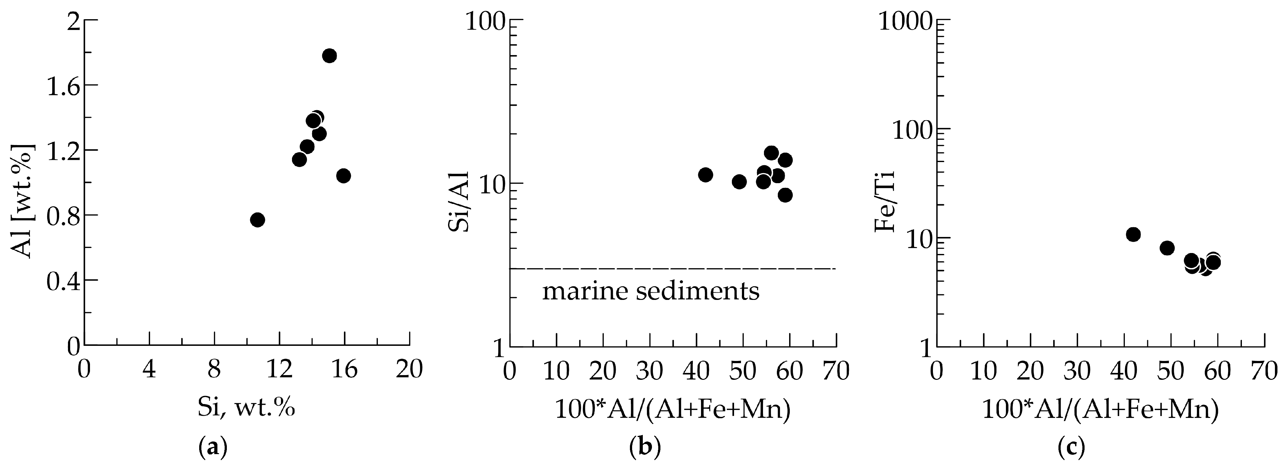
4.3. Characterization of Major and Trace Elements in Sinking Matter to Identify Hydrothermal Contribution

Both moorings demonstrate an increase in excess iron (Fe_ex) with depth. The Fe_ex content varies between 0.13% and 1.01% in the TW field, and between 0.26% and 0.43% in the SM field. The maximum Fe_ex content is observed at depths of 450 and 520 m within the TW field. The proportion of Fe_ex in the sinking matter varies from a minimum of 26% to a maximum of 63% of the total iron content. The EF values for Fe do not exceed the value of three at any water level, with the maximum value of 2.7 occurring at a depth of 520 m of the TW field. This indicates a significant proportion of lithogenic matter in sinking particles. The elevated iron concentration observed in the TW field plume is a consequence of the higher content of iron-silicate oxyhydroxides, with Fe concentrations reaching 45 wt.% (Table S3). The content of Fe-Si oxyhydroxides and their Fe concentration (up to 37 wt.%) were found to be lower in the sinking matter of the SM field than in the sinking matter of the TW vent field. In the composition of Fe-Si oxyhydroxides, Ca in both fields and P in the SM vent field are reported as simple substitutions. It is well established that Fe oxyhydroxide particles are capable of absorbing Ca and P from seawater [7]. Despite the fact that pyrite crystals were observed among the sinking particles from both sites, there is evidence from microscopic examination that Fe-Si oxyhydroxide precipitation is more prevalent than Fe sulfide precipitation.

The highest concentration of manganese (Mn) is observed in the 450–470 m layer, particularly in the particles of the TW plume (up to 1472 ppm). This may be attributed to the oxidation of Mn, which shows a higher concentration in the hydrothermal plume and its precipitation from the solution [80]. The lack of clearly identified Mn-bearing minerals based on SEM may suggest that this element exists as a dispersed nanoparticle phase. According to [5], Mn and abiogenic gasses (CH₄, ³He) had similar elevated concentrations coinciding with density changes close to 500 m. In TW vent field samples, synchronously with the increase in Mn concentration, there is an increase in the concentration and EF of Cs, As, Rb, and Ce, which are co-precipitated with Mn oxyhydroxide particles. This suggests scavenging processes [81].

The concentration of Cd, Zn, and P in sinking particles is slightly elevated in the upper water layer above 150 m. Thus, high concentrations of these elements in the surface water are due to their occurrence in the biogenic particles [26] that are abundant in these productive waters with Chl-a concentrations of 1–2 mg/m³.

The high Al content and the close relationship between the Si and Al content (R² = 0.71, n = 8) indicate a significant role of aluminosilicates in the composition of sinking material, which is supported by the EDS data. A number of elements that are associated with lithogenic matter and included in the rock-forming (groups of olivines, pyroxenes, plagioclases, etc.) and accessory minerals of igneous rocks are characterized by a vertical distribution similar to that of aluminum: Ti, V, Zr, Hf, Nb, Ta, Ni, most of REE (except Eu) and Th. The content of these elements reaches its maximum value at depths of 100–200 m below the surface water layer. This serves as a proxy for the absence of the benthic nepheloid layer, as no discernible increase in the concentration of these elements due to the resuspension of surface bottom sediments was observed. The elevated concentration of Ni and Cr (and their correlation with Ta, Y, and Nb) in the sinking material as well as in the background bottom sediments outside the hydrothermal fields [39] can be attributed to the influence of the Jan Mayen rocks [46,82], which are enriched in incompatible elements. In the near-bottom layers, in addition to the organo-mineral aggregates of sinking particles from the euphotic zone of the water column, an abundance of minerals of hydrothermal genesis (barite, gypsum; Fe, Cu, and Zn sulfides; and Fe-Si oxyhydroxides) is observed. Elevated concentrations of Fe, Mn, Ba, Cu, Pb, and Cd were previously observed in the SPM of the JMVFs in the benthic and intermediate layers [80]. The sinking particles of the studied fields represent a mixture of different components and form a specific population of particles including the pelagic/hemipelagic background particles, volcanogenic particles and particles derived from Jan Mayen basalts and basalts associated with submarine eruptions, and hydrothermally derived particles [39,83].

The Ba content involved in barite formation is 2.5 times higher in the composition of sinking particles from the SM vent field than from the TW vent field. The SEM examination demonstrated that barites occur in a typical rosette morphology consisting of cross-cut tabular crystals, with sizes varying from 50 to 120 µm (Figure S1c,g–i). Hydrothermal barite is a primary precipitate of Ba-rich pure (mantle-derived) hydrothermal fluids interacting and mixing with sulfate-rich seawater [84,85,86]. Non-radiogenic Sr (as well as Ba) is leached from the oceanic crust (basalt). EDS microanalysis for achieve the chemical characterization of barite has shown average contents of 52.79 ± 9.33% for Ba, 14.72 ± 0.78% for S, and 2.81 ± 1.67% for Sr on SM (Table S2) and 44.10 ± 1.85% for Ba, 17.17 ± 1.22% for S, and 2.84 ± 0.79% for Sr on TW (Table S5). More than 90% of barite consists of Ba and SO₄, and the Ba/S molar ratio of the crystals (range from 0.52 to 1.08) is close to that of pure barite. Using the stoichiometric ratio and subtracting the Ba contribution from settling from upper active layer particles, the vertical flux of hydrothermal barite can be calculated to be 694 and 2103 µg/m²/day at the TW and SM vents, respectively.

The particles of the studied buoyant plumes are characterized by the following association of chalcophilic trace elements Zn, Fe, Cd, Cu, Pb, V, and Tl. Among the sulfide minerals, zinc sulfides (sphalerites) are the most significant. Sulfides of Fe, Cu, etc. are less substantial. It has been observed by Stensland et al. [5] that copper and iron exhibit similar profiles with peaks at two distinct depths of the water column: approximately 500 and 600 m. A similar pattern is observed in our samples, wherein Fe forms an association with Cu, Co, and V, and enriches the sediment at the same depths. The SEM data indicate that the collomorphic (bud-shaped) porous microconcretions of Fe sulfides form a mineral association with the sulfides of Zn and other sulfide-forming elements. Only pyrite and sphalerite form octahedra and cuboctahedra of 3–6 µm in diameter. Hydrothermally derived barite forms a stable mineral association with sulfides. The mineral barite has been previously observed in association with zinc sulfides in the bottom sediments of the JMVFs [39,83]. Using the stoichiometric ratio and subtracting the flux of Zn from the upper layers, it would be possible to estimate the flux of sphalerite, which was as high as 313 and 1676 µg/m²/day at the TW and SM vent sites, respectively.

The particle compositions of the studied buoyant plumes appear to be related to the temperature of the fluids in the studied vent fields. Consequently, the maximum fluid temperature of both hydrothermal vent fields reaches approximately 270 °C [37,39]; however, irregularly shaped barite-silica chimneys with large flanges that emit low-temperature fluids are also found on the SM vent field [37].

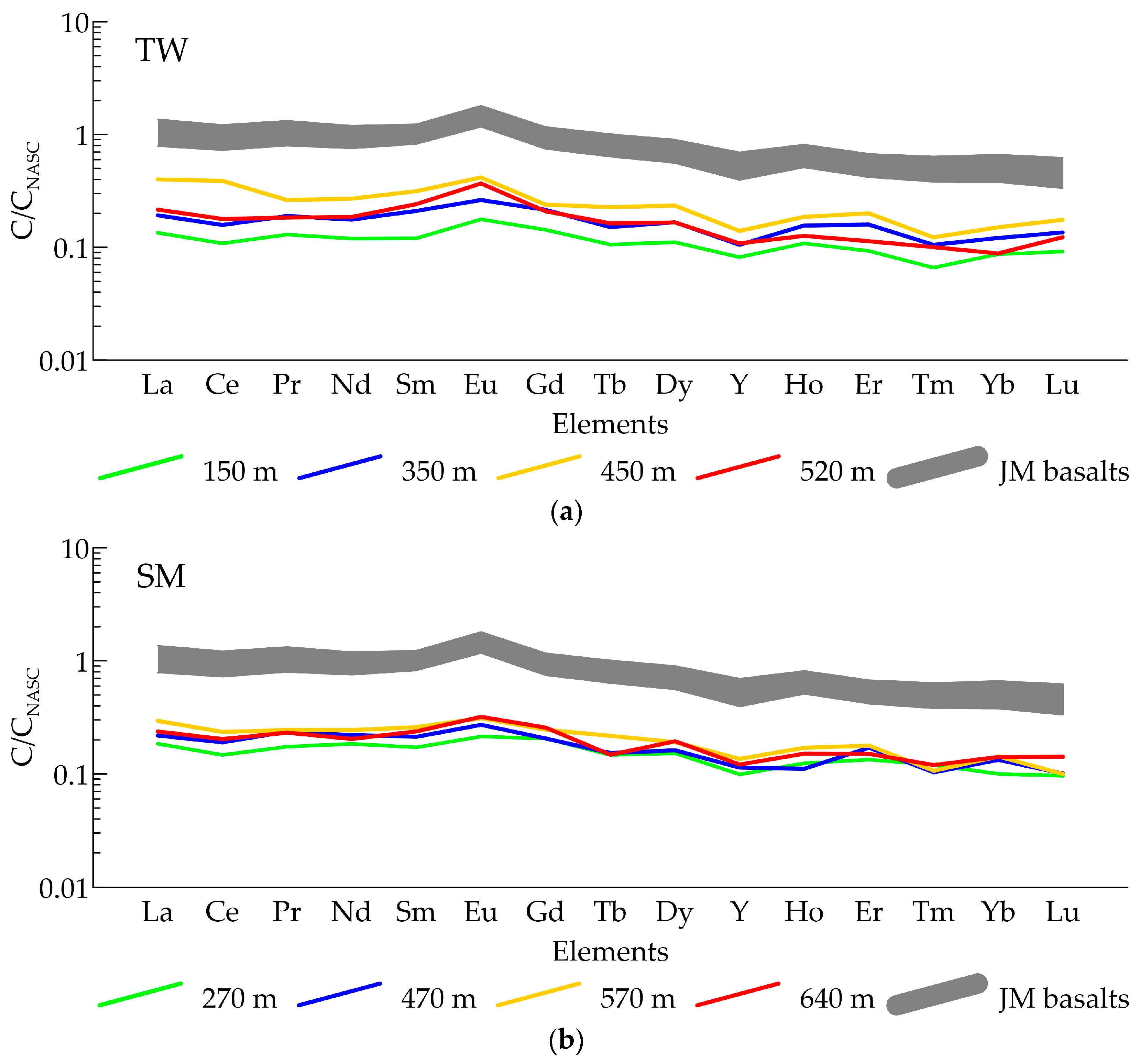
4.4. REE in Particle Fluxes as a Traces of Hydrotermaly Derived Particles

In general, the REE spectrum of the trapped material is very similar to that of alkaline Jan Mayen basalts (Figure 8), as reported by Haase et al. [68], indicating a substantial contribution of this material. However, the total REE content is 4–6 times lower than that in basalts. This can be explained by the admixture of organic and carbonate matter and the admixture of hydrothermally derived sulfide minerals, which have the effect of reducing the REE content when introduced into the sinking matter. REE patterns can be influenced by minor aluminosilicate detritus due to the low REE content in the hydrothermal precipitates [87]. Negative cerium anomalies (Ce_an = 0.82–0.89) suggest the scavenging of REE by suspended matter in the buoyant plume from seawater. As previously reported, significant REE scavenging must mostly occur after the deposition of suspended hydrothermal precipitates from the water column [81,87,88]. This is why the negative cerium anomaly is not very pronounced. There is also one sample with a positive cerium anomaly (Ce_an = 1.17). It was sampled at the TW vent site at a depth of 450 m, where the Mn content is high (Table 2). This indicates the presence of a significant amount of hydrous manganese oxides in the sample. In general, both the studied vent sites are characterized by a decrease in Ce_an values at the upper layers of the water column, indicating an increasing in the influence of the dissolved REEs from seawater with decreasing depth, as reported by Dubinin [65,89]. A number of indicator ratios (light to heavy REEs ratio, Eu_an) suggest a potential hydrothermal influence of the water layer up to 100 m from the seafloor [90].

The influence of hydrothermal buoyant plume is most pronounced at 30 m from the bottom, but is also evident at virtually all the sampling depths in the water column. This may be due to the delivery of nanoparticles during the collapse of gas bubbles due to pressure reduction during surfacing [5]. The positive europium anomaly in the water column above 100 m from the seafloor may be partly due to the supply of Jan Mayen basaltic material with the Jan Mayen Current. Thus, basaltic tephra has been identified along the entire length of a bottom sediment core sampled in the southeast of the island [91], and is also abundant in the surface sediments of the Jan Mayen AVR [39,83].

4.5. Fluxes of Hydrothermally Derived Elements and Specific Features of Studied Hydrothermal Buoyant Plumes

The ratio of the individual element fluxes in the bottom layer to the overlying background fluxes is higher in the SM field, with the exception of Fe (Table 5), which is likely due to differences in the locations of the studied vent fields in relation to the AVR. In addition, the SM vent field is characterized by two types of venting: white smokers and clear plumes with a wide temperature range from 50 to 270 °C. The extensive yellow-brown Fe oxyhydroxide deposits and iron enrichment of the bottom sediments observed in the TW vent field area have been previously documented in our work [39] and in the literature [37,45]. Furthermore, the enrichment of the water column with particulate and dissolved iron, delivered with gas bubbles above the TW vent field, has also been reported in [5]. It has been demonstrated that metal migration occurs above the hydrothermal plume, specifically on the hydrate-coated gas bubbles. As the bubbles rise, the hydrates are disrupted, resulting in the release of metal-rich nanoparticles. Further coagulation of nanoparticles can result in the enrichment of the sedimentary matter with metals such as Co, V, Ga, and Cu.

Comparison of the elemental fluxes with the available data for a number of other hydrothermal vent fields (Table 5, [13,15,28,29,31,73]) revealed that the fluxes of Fe, Cu, and Zn in the JMVFs are several orders of magnitude lower than those observed in other vent fields. This phenomenon has previously been demonstrated in the context of trace element concentrations in suspended particulate matter in the vicinity of the TW vent field [39]. At the same time, the Ba flux is comparable to other vent fields and even exceeds its magnitude at the Broken Spur vent field. Ba content in the sinking matter of the studied TW and SM vent fields is one of the highest among the known low- and medium-temperature hydrothermal systems. The ratio Ba in the flux is the closest to that of the Lucky Strike vent field [15].

The MAR hydrothermal vent fields, located at 14°45′–37°30′ N, are also associated with basaltic volcanism and occur at variable depths, ranging from 850 to 3670 m. Primary fluid temperatures have been observed to range from 363 °C to 152 °C (Table 5). It has been demonstrated that the fluids of the Lucky Strike and Menezes Gwen vent fields exhibit compositional differences from other MAR hydrothermal fields located south of the Azores hotspot. These differences include a lower temperature; a high pH value (up to 5); a lower concentration of Cl, Na, Fe, Li, and Cu; and an enrichment of Ba, Zn, Pb, Cs, and Rb. These characteristics are typically attributed to the elevated concentration of the aforementioned elements in the basalts that were initially emplaced near the Azores hotspot [39,92]. Nevertheless, despite the proximity of the P-T conditions of the JMVFs to those of the Lucky Strike and Menezes Gwen vent fields and to the basalts involved in hydrothermal particle formation, the fluxes and concentrations of these elements in the TW and SM trapped matter differ to a greater extent (Table 5). In the deeper waters (>3000 m) and at high temperatures (>350 °C) of the Broken Spur and TAG vent fields, the flux of barium is minimal among all the MAR vent sites. Increasing fluxes of Cu and Zn are observed here.

It is also possible that the observed differences in the magnitude of the total fluxes and fluxes of hydrothermally derived elements may be attributed to variations in the conditions of sinking particles collected by sediment traps at different vent fields. The moorings were deployed at varying distances from the vents and from the bottom of the seafloor [13,15,28,29,31,73].

In the course of our study, the temperature of the water in the lower layer of the TW vent field exhibited a number of increases, which resulted in the occurrence of the plume impact on the traps on a number of occasions (Figure 5). In the SM vent field, such impacts were recorded on just four occasions during the running time of the trap. They were recorded once a day during high tide. This phenomenon can be attributed to a change in the direction of plume transport under the influence of the tide and a change in the temperature regime of the source, which depends on the phase of the tide. This phenomenon has also been observed at the Lucky Strike vent field [93]. At the same time, the fluxes of hydrothermally derived elements and minerals, particularly barium (Ba) and zinc (Zn), and their respective ores, barite and sphalerite, exhibited significantly elevated levels precisely at the SM vent field. In general, these facts indicate a higher particle release by white smokers at the SM vent field compared to the TW vent field. The data obtained emphasize the circulation of several immiscible phases and fluids of slightly different compositions in the studied hydrothermal systems within the Jan Mayen vent field area and possibly the different degrees of maturity of the studied ore-generating hydrothermal systems.

5. Conclusions

This study examines sinking particle fluxes and their composition at two white smoker venting sites (Troll Wall and Soria Moria) of the JMVFs located at the AVR and forming volcanogenic massive sulfide deposits, dominated by barite-sphalerite mineralization. Our findings contribute to the limited number of studies investigating sinking particle fluxes from buoyant and neutrally buoyant hydrothermal vent fields in the ocean. The supply of hydrothermally derived matter is accompanied by normal pelagic/hemipelagic sedimentation, which is dominated by biogenic particles, especially in the upper water layers, and basaltic particles from the seafloor and Jan Mayen rocks. In general, the JMVFs exhibit relatively low plume turbidity and hence, low vertical fluxes of sinking particles, which is markedly lower than at other hydrothermal vent fields of the MAR and EPR (only 103 mg/m²/day against 264–11,589 mg/m²/day [13,15,28,29,31,71,72,73]). The hydrothermal plume propagates subhorizontally in a northeasterly direction (~45°) within a layer that extends no more than 100 m from the bottom. The impact of hydrothermally derived particles is most evident at a depth of 30 m above the seafloor. The transportation of buoyancy hydrothermal plumes was significantly affected by tidal motion. Nevertheless, the influence of hydrothermally derived particles is observed for certain parameters in almost the entire water column from the bottom to the subsurface layers due to the relative shallowness of the Jan Mayen vent field area.

Hydrothermally derived particles were represented by a low- to medium-temperature mineral association including barite, sphalerite, pyrite, chalcopyrite, gypsum, and non-crystalline Fe-Si oxyhydroxides. The vertical flux of hydrothermal barite at the SM is ~3 times higher than at the TW: 2103 µg/m²/day and 694 µg/m²/day, respectively. The widespread occurrence of barite at the JMVFs suggests the proximity of the volcanic centers of the region to the enriched MORB type. The flux of sphalerite, the next abundant hydrothermal mineral, at the SM is ~5 times higher than at the TW: 1676 µg/m²/day and 313 µg/m²/day, respectively. Therefore, despite the proximity of the studied vent sites to each other and similar fluid features characteristic of volcanogenic massive sulfide deposits, differences in the composition of the settling hydrothermal matter of the TW and SM fields were clearly identified. These differences were observed in the elemental composition of the particles, with some specialization evident. SM vent field is distinguished by a more pronounced influx of sedimentary matter compared to the TW field, accompanied by elevated fluxes of Zn and Ba. On the contrary, the TW field exhibits elevated values of Fe and Mn fluxes. This phenomenon is likely attributed to the absence of a single end-member fluid and the presence of sources of varying configuration and intensity, with differing fluid temperatures, within the studied fields. Furthermore, data obtained emphasize the circulation of several immiscible phases and fluids of slightly different compositions in the studied hydrothermal systems. The SM vent field, located at the top of a small volcanic rift, appears to be characterized by stronger activity and more influence of the enriched MORB-type mantle source than the TW vent field, which is confined to a fault bounding the rift valley wall through a large central volcano. In terms of the sinking matter composition, the TW and SM vent fields are most similar to the Menez Gwen and Lucky Strike vent fields affected by the Azores hotspot. Our study yields important geochemical and mineralogical data regarding hydrothermally derived sinking particles that provide a unique perspective on the mafic-hosted hydrothermal settings affected by hotspots.

References

1. Baker, E.T.; German, C.R. On the Global Distribution of Hydrothermal Vent Fields. In Mid-Ocean Ridges: Hydrothermal Interactions Between the Lithosphere and Oceans; Geophysical Monograph Series; American Geophysical Union: Washington, DC, USA, 2004; Volume 148, pp. 245–266. [Google Scholar]
2. Lein, A.Y.; Bogdanov, Y.A.; Lisitzin, A.P. Processes of Hydrothermal Ore Genesis in the World Ocean: The Results of 35 Years of Research. Dokl. Earth Sci. 2016, 466, 38–41. [Google Scholar] [CrossRef]
3. Lupton, J.E.; Delaney, J.R.; Johnson, H.P.; Tivey, M.K. Entrainment and Vertical Transport of Deep-Ocean Water by Buoyant Hydrothermal Plumes. Nature 1985, 316, 621–623. [Google Scholar] [CrossRef]
4. Speer, K.G.; Rona, P.A. A Model of an Atlantic and Pacific Hydrothermal Plume. J. Geophys. Res. Ocean. 1989, 94, 6213–6220. [Google Scholar] [CrossRef]
5. Stensland, A.; Baumberger, T.; Lilley, M.D.; Okland, I.E.; Dundas, S.H.; Roerdink, D.L.; Thorseth, I.H.; Pedersen, R.B. Transport of Carbon Dioxide and Heavy Metals from Hydrothermal Vents to Shallow Water by Hydrate-Coated Gas Bubbles. Chem. Geol. 2019, 513, 120–132. [Google Scholar] [CrossRef]
6. Gartman, A.; Findlay, A.J. Impacts of Hydrothermal Plume Processes on Oceanic Metal Cycles and Transport. Nat. Geosci. 2020, 13, 396–402. [Google Scholar] [CrossRef]
7. Feely, R.A.; Gendron, J.F.; Baker, E.T.; Lebon, G.T. Hydrothermal Plumes along the East Pacific Rise, 8 40′ to 11 50′ N: Particle Distribution and Composition. Earth Planet. Sci. Lett. 1994, 128, 19–36. [Google Scholar] [CrossRef]
8. Butterfield, D.A.; Massoth, G.J.; McDuff, R.E.; Lupton, J.E.; Lilley, M.D. Geochemistry of Hydrothermal Fluids from Axial Seamount Hydrothermal Emissions Study Vent Field, Juan de Fuca Ridge: Subseafloor Boiling and Subsequent Fluid-rock Interaction. J. Geophys. Res. Solid Earth 1990, 95, 12895–12921. [Google Scholar] [CrossRef]
9. Gurvich, E.G. Metalliferous Sediments of the World Ocean: Fundamental Theory of Deep-Sea Hydrothermal Sedimentation; Springer: Berlin/Heidelberg, Germany, 2006; ISBN 3-540-27869-9. [Google Scholar]
10. Klevenz, V.; Bach, W.; Schmidt, K.; Hentscher, M.; Koschinsky, A.; Petersen, S. Geochemistry of Vent Fluid Particles Formed during Initial Hydrothermal Fluid–Seawater Mixing along the Mid-Atlantic Ridge. Geochem. Geophys. Geosyst. 2011, 12, Q0AE05. [Google Scholar] [CrossRef]
11. Lisitzin, A.P. Oceanic Sedimentation: Lithology and Geochemistry; American Geophysical Union: Washington, DC, USA, 1996. [Google Scholar]
12. German, C.R.; Seyfried, W.E. Hydrothermal Processes. In Treatise on Geochemistry, 2nd ed.; Elsevier: Amsterdam, The Netherlands, 2014; Volume 8, pp. 191–233. ISBN 978-0-08-098300-4. [Google Scholar]
13. Khripounoff, A.; Vangriesheim, A.; Crassous, P.; Segonzac, M.; Colaço, A.; Desbruyeres, D.; Barthelemy, R. Particle Flux in the Rainbow Hydrothermal Vent Field (Mid-Atlantic Ridge): Dynamics, Mineral and Biological Composition. J. Mar. Res. 2001, 59, 633–656. [Google Scholar] [CrossRef]
14. German, C.R.; Sparks, R.S.J. Particle Recycling in the TAG Hydrothermal Plume. Earth Planet. Sci. Lett. 1993, 116, 129–134. [Google Scholar] [CrossRef]
15. Khripounoff, A.; Comtet, T.; Vangriesheim, A.; Crassous, P. Near-Bottom Biological and Mineral Particle Flux in the Lucky Strike Hydrothermal Vent Area (Mid-Atlantic Ridge). J. Mar. Syst. 2000, 25, 101–118. [Google Scholar] [CrossRef]
16. Thurnherr, A.M.; St. Laurent, L.C. Turbulence Observations in a Buoyant Hydrothermal Plume on the East Pacific Rise. Oceanography 2012, 25, 180–181. [Google Scholar] [CrossRef]
17. Haymon, R.M.; Kastner, M. Hot Spring Deposits on the East Pacific Rise at 21 N: Preliminary Description of Mineralogy and Genesis. Earth Planet. Sci. Lett. 1981, 53, 363–381. [Google Scholar] [CrossRef]
18. Baker, E.T.; Lavelle, J.W.; Massoth, G.J. Hydrothermal Particle Plumes over the Southern Juan de Fuca Ridge. Nature 1985, 316, 342–344. [Google Scholar] [CrossRef]
19. Dymond, J.; Lyle, M. Particle Fluxes in the Ocean and Implications for Sources and Preservation of Ocean Sediments. In Material Fluxes on the Surface of the Earth; The National Academies Press: Washington, DC, USA, 1994; pp. 125–142. [Google Scholar]
20. German, C.R.; Casciotti, K.A.; Dutay, J.-C.; Heimbürger, L.-E.; Jenkins, W.J.; Measures, C.I.; Mills, R.A.; Obata, H.; Schlitzer, R.; Tagliabue, A. Hydrothermal Impacts on Trace Element and Isotope Ocean Biogeochemistry. Philos. Trans. R. Soc. Math. Phys. Eng. Sci. 2016, 374, 20160035. [Google Scholar] [CrossRef] [PubMed]
21. Edmonds, H.N.; German, C.R. Particle Geochemistry in the Rainbow Hydrothermal Plume, Mid-Atlantic Ridge. Geochim. Cosmochim. Acta 2004, 68, 759–772. [Google Scholar] [CrossRef]
22. Toner, B.M.; Marcus, M.A.; Edwards, K.J.; Rouxel, O.; German, C.R. Measuring the Form of Iron in Hydrothermal Plume Particles. Oceanography 2012, 25, 209–212. [Google Scholar] [CrossRef]
23. Von Damm, K.L. Seafloor Hydrothermal Activity: Black Smoker Chemistry and Chimneys. Annu. Rev. Earth Planet. Sci. 1990, 18, 173–204. [Google Scholar] [CrossRef]
24. Guieu, C.; Bonnet, S.; Petrenko, A.; Menkes, C.; Chavagnac, V.; Desboeufs, K.; Maes, C.; Moutin, T. Iron from a Submarine Source Impacts the Productive Layer of the Western Tropical South Pacific (WTSP). Sci. Rep. 2018, 8, 9075. [Google Scholar] [CrossRef] [PubMed]
25. Holmes, T.M.; Chase, Z.; van der Merwe, P.; Townsend, A.T.; Bowie, A.R. Detection, Dispersal and Biogeochemical Contribution of Hydrothermal Iron in the Ocean. Mar. Freshw. Res. 2017, 68, 2184–2204. [Google Scholar] [CrossRef]
26. Horner, T.J.; Little, S.H.; Conway, T.M.; Farmer, J.R.; Hertzberg, J.E.; Janssen, D.J.; Lough, A.J.M.; McKay, J.L.; Tessin, A.; Galer, S.J. Bioactive Trace Metals and Their Isotopes as Paleoproductivity Proxies: An Assessment Using GEOTRACES-era Data. Glob. Biogeochem. Cycles 2021, 35, e2020GB006814. [Google Scholar] [CrossRef]
27. Cobler, R.; Dymond, J. Sediment Trap Experiment on the Galapagos Spreading Center, Equatorial Pacific. Science 1980, 209, 801–803. [Google Scholar] [CrossRef]
28. Lukashin, V.N.; Rusakov, V.Y.; Lisitzin, A.P.; Lein, A.Y.; Isaeva, A.B.; Serova, V.V.; Karpenko, A.A. Study of Particle Fluxes in the Broken Spur Hydrothermal Vent Field (29°N, Mid-Atlantic Ridge). Explor. Min. Geol 1999, 8, 341–353. [Google Scholar]
29. Khripounoff, A.; Alberic, P. Settling of Particles in a Hydrothermal Vent Field (East Pacific Rise 13 N) Measured with Sediment Traps. Deep Sea Res. Part Oceanogr. Res. Pap. 1991, 38, 729–744. [Google Scholar] [CrossRef]
30. Desbruyères, D.; Almeida, A.; Biscoito, M.; Comtet, T.; Khripounoff, A.; Le Bris, N.; Sarradin, P.M.; Segonzac, M. A Review of the Distribution of Hydrothermal Vent Communities along the Northern Mid-Atlantic Ridge: Dispersal vs. Environmental Controls. In Proceedings of the Island, Ocean and Deep-Sea Biology: Proceedings of the 34th European Marine Biology Symposium, Ponta Delgada, Azores, Portugal, 13–17 September 1999; Springer: Berlin/Heidelberg, Germany, 2000; pp. 201–216. [Google Scholar]
31. German, C.; Colley, S.; Palmer, M.R.; Khripounoff, A.; Klinkhammer, G.P. Hydrothermal Plume-Particle Fluxes at 13 N on the East Pacific Rise. Deep Sea Res. Part Oceanogr. Res. Pap. 2002, 49, 1921–1940. [Google Scholar] [CrossRef]
32. Beaulieu, S.E.; Mullineaux, L.S.; Adams, D.K.; Mills, S.W. Comparison of a Sediment Trap and Plankton Pump for Time-series Sampling of Larvae near Deep-sea Hydrothermal Vents. Limnol. Oceanogr. Methods 2009, 7, 235–248. [Google Scholar] [CrossRef]
33. Sylvan, J.B.; Pyenson, B.C.; Rouxel, O.; German, C.R.; Edwards, K.J. Time-series Analysis of Two Hydrothermal Plumes at 9° 50′ N East Pacific Rise Reveals Distinct, Heterogeneous Bacterial Populations. Geobiology 2012, 10, 178–192. [Google Scholar] [CrossRef]
34. Kiyokawa, S.; Ueshiba, T. Rapid Sedimentation of Iron Oxyhydroxides in an Active Hydrothermal Shallow Semi-Enclosed Bay at Satsuma Iwo-Jima Island, Kagoshima, Japan. Sediment. Geol. 2015, 319, 98–113. [Google Scholar] [CrossRef]
35. Pedersen, R.B.; Thorseth, I.H.; Hellevang, B.; Schultz, A.; Taylor, P.; Knudsen, H.P.; Steinsbu, B.O. Two Vent Fields Discovered at the Ultraslow Spreading Arctic Ridge System. In AGU Fall Meeting Abstracts; American Geophysical Union: Washington, DC, USA, 2005; Volume 2005, p. OS21C-01. [Google Scholar]
36. Pedersen, R.B.; Bjerkgård, T. Seafloor Massive Sulphides in Arctic Waters. In Mineral Resources in the Arctic; Geological Survey of Norway: Trondheim, Norway, 2016; Volume 1, pp. 209–216. [Google Scholar]
37. Pedersen, R.B.; Thorseth, I.H.; Nygård, T.E.; Lilley, M.D.; Kelley, D.S. Hydrothermal Activity at the Arctic Mid-Ocean Ridges. Geophys. Monogr. Ser. 2010, 188, 67–89. [Google Scholar]
38. Dahle, H.; Le Moine Bauer, S.; Baumberger, T.; Stokke, R.; Pedersen, R.B.; Thorseth, I.H.; Steen, I.H. Energy Landscapes in Hydrothermal Chimneys Shape Distributions of Primary Producers. Front. Microbiol. 2018, 9, 1570. [Google Scholar] [CrossRef] [PubMed]
39. Kravchishina, M.D.; Lein, A.Y.; Boev, A.G.; Prokofiev, V.Y.; Starodymova, D.P.; Dara, O.M.; Novigatsky, A.N.; Lisitzin, A.P. Hydrothermal Mineral Assemblages at 71° N of the Mid-Atlantic Ridge (First Results). Oceanology 2019, 59, 941–959. [Google Scholar] [CrossRef]
40. Juliani, C.; Ellefmo, S.L. Probabilistic Estimates of Permissive Areas for Undiscovered Seafloor Massive Sulfide Deposits on an Arctic Mid-Ocean Ridge. Ore Geol. Rev. 2018, 95, 917–930. [Google Scholar] [CrossRef]
41. Blindheim, J.; Rey, F. Water-Mass Formation and Distribution in the Nordic Seas during the 1990s. ICES J. Mar. Sci. 2004, 61, 846–863. [Google Scholar] [CrossRef]
42. Blindheim, J.; Osterhus, S. The Nordic Seas, Main Oceanographic Features. Geophys. Monogr.-Am. Geophys. Union 2005, 158, 11. [Google Scholar]
43. Dick, H.J.; Lin, J.; Schouten, H. An Ultraslow-Spreading Class of Ocean Ridge. Nature 2003, 426, 405–412. [Google Scholar] [CrossRef] [PubMed]
44. Kandilarov, A.; Mjelde, R.; Pedersen, R.-B.; Hellevang, B.; Papenberg, C.; Petersen, C.-J.; Planert, L.; Flueh, E. The Northern Boundary of the Jan Mayen Microcontinent, North Atlantic Determined from Ocean Bottom Seismic, Multichannel Seismic, and Gravity Data. Mar. Geophys. Res. 2012, 33, 55–76. [Google Scholar] [CrossRef]
45. Johannessen, K.C.; Vander Roost, J.; Dahle, H.; Dundas, S.H.; Pedersen, R.B.; Thorseth, I.H. Environmental Controls on Biomineralization and Fe-Mound Formation in a Low-Temperature Hydrothermal System at the Jan Mayen Vent Fields. Geochim. Cosmochim. Acta 2017, 202, 101–123. [Google Scholar] [CrossRef]
46. Elkins, L.J.; Hamelin, C.; Blichert-Toft, J.; Scott, S.R.; Sims, K.W.W.; Yeo, I.A.; Devey, C.W.; Pedersen, R.B. North Atlantic Hotspot-Ridge Interaction near Jan Mayen Island. Geochem. Perspect. Lett. 2016, 2, 55–67. [Google Scholar] [CrossRef]
47. Geli, L.; Renard, V.; Rommevaux, C. Ocean Crust Formation Processes at Very Slow Spreading Centers: A Model for the Mohns Ridge, near 72° N, Based on Magnetic, Gravity, and Seismic Data. J. Geophys. Res. 1994, 99, 2995–3013. [Google Scholar] [CrossRef]
48. Cherkashev, G.A.; Gusev, E.A.; Zhirnov, E.A.; Tamaki, K.; Kurevits, D.; Okino, K.; Sato, H.; Baranov, B.V.; Egorov, A.V.; German, K. The Knipovich Ridge Rift Zone: Evidence from the Knipovich-2000 Expedition. Dokl. Earth Sci. 2001, 378, 420–423. [Google Scholar]
49. Kokhan, A.V.; Dubinin, E.P.; Grokholsky, A.L. Geodynamical Peculiarities of Structure-Forming in Arctic and Polar Atlantic Spreading Ridges. Bull. Kamchatka Reg. Assoc. 2012, 19, 59–77. [Google Scholar]
50. Reimers, H. The Morphology of the Mohn’s Ridge-with Special Focus on Listric and Detachment Faults and Their Link to the Formation of Seafloor-Massive Sulfides. Master’s Thesis, NTNU, Trondheim, Norway, 2017. [Google Scholar]
51. Klyuvitkin, A.A.; Kravchishina, M.D.; Nemirovskaya, I.A.; Baranov, B.V.; Kochenkova, A.I.; Lisitzin, A.P. Studies of Sediment Systems of the European Arctic during Cruise 75 of the R/V Akademik Mstislav Keldysh. Oceanology 2020, 60, 421–423. [Google Scholar] [CrossRef]
52. Lukashin, V.N.; Klyuvitkin, A.A.; Lisitzin, A.P.; Novigatsky, A.N. The MSL-110 Small Sediment Trap. Oceanology 2011, 51, 699–703. [Google Scholar] [CrossRef]
53. Stensland, A. Dissolved Gases in Hydrothermal Plumes from Artic Vent Fields. Master’s Thesis, The University of Bergen, Bergen, Norway, 2013. [Google Scholar]
54. Klyuvitkin, A.A.; Novigatsky, A.N.; Politova, N.V.; Koltovskaya, E.V. Studies of Sedimentary Matter Fluxes along a Long-Term Transoceanic Transect in the North Atlantic and Arctic Interaction Area. Oceanology 2019, 59, 411–421. [Google Scholar] [CrossRef]
55. Klyuvitkin, A.A.; Kravchishina, M.D.; Novigatsky, A.N.; Politova, N.V.; Bulokhov, A.V.; Gulev, S.K. First Data on Vertical Particle Fluxes and Environmental Conditions in the Northern Segment of the Mohns Ridge, Norwegian Sea. Dokl. Earth Sci. 2023, 513, 1204–1210. [Google Scholar] [CrossRef]
56. Holm-Hansen, O.; Riemann, B. Chlorophyll a Determination: Improvements in Methodology. Oikos 1978, 30, 438–447. [Google Scholar] [CrossRef]
57. Kravchishina, M.D.; Lisitsyn, A.P.; Klyuvitkin, A.A.; Novigatsky, A.N.; Politova, N.V.; Shevchenko, V.P. Suspended Particulate Matter as a Main Source and Proxy of the Sedimentation Processes. In Sedimentation Processes in the White Sea: The White Sea Environment Part II; Springer: Cham, Switzerland, 2018; pp. 13–48. [Google Scholar]
58. Gelman, E.M.; Starobina, I.Z. Photometric Methods for Determining the Rock Forming Elements in Ores, Rocks and Minerals; GEOKHI AS USSR: Moscow, Russia, 1976; pp. 1–69. (In Russian) [Google Scholar]
59. Rudnick, R.L.; Gao, S. Composition of the Continental Crust. In Treatise on Geochemistry, 2nd ed.; Elsevier: Amsterdam, The Netherlands, 2014; Volume 4. [Google Scholar] [CrossRef]
60. Lukashin, V.N.; Krechik, V.A.; Klyuvitkin, A.A.; Starodymova, D.P. Geochemistry of Suspended Particulate Matter in the Marginal Filter of the Pregolya River (Baltic Sea). Oceanology 2018, 58, 856–869. [Google Scholar] [CrossRef]
61. Honjo, S.; Krishfield, R.A.; Eglinton, T.I.; Manganini, S.J.; Kemp, J.N.; Doherty, K.; Hwang, J.; McKee, T.K.; Takizawa, T. Biological Pump Processes in the Cryopelagic and Hemipelagic Arctic Ocean: Canada Basin and Chukchi Rise. Prog. Oceanogr. 2010, 85, 137–170. [Google Scholar] [CrossRef]
62. Starodymova, D.P.; Kotova, E.I.; Shevchenko, V.P.; Titova, K.V.; Lukyanova, O.N. Winter Atmospheric Deposition of Trace Elements in the Arkhangelsk Region (NW Russia): Insights into Environmental Effects. Atmos. Pollut. Res. 2024, 15, 102310. [Google Scholar] [CrossRef]
63. Rollinson, H.R.; Pease, V. Using Geochemical Data: To Understand Geological Processes; Cambridge University Press: Cambridge, UK, 2021; ISBN 1-108-74584-9. [Google Scholar]
64. Gromet, L.P.; Haskin, L.A.; Korotev, R.L.; Dymek, R.F. The “North American Shale Composite”: Its Compilation, Major and Trace Element Characteristics. Geochim. Cosmochim. Acta 1984, 48, 2469–2482. [Google Scholar] [CrossRef]
65. Dubinin, A.V. Rare Earth Element Geochemistry in the Ocean; Nauka: Moscow, Russia, 2006; ISBN 5-02-033745-5. (In Russian) [Google Scholar]
66. Kravchishina, M.D.; Prokofiev, V.Y.; Dara, O.M.; Baranov, B.V.; Klyuvitkin, A.A.; Iakimova, K.S.; Kalgin, V.Y.; Lein, A.Y. Fluid Inclusion Studies of Barite Disseminated in Hydrothermal Sediments of the Mohns Ridge. Minerals 2023, 13, 1117. [Google Scholar] [CrossRef]
67. Boström, K.; Peterson, M.N.A.; Joensuu, O.; Fisher, D.E. Aluminum-poor Ferromanganoan Sediments on Active Oceanic Ridges. J. Geophys. Res. 1969, 74, 3261–3270. [Google Scholar] [CrossRef]
68. Haase, K.M.; Devey, C.W.; Mertz, D.F.; Stoffers, P.; Garbe-Schönberg, D. Geochemistry of Lavas from Mohns Ridge, Norwegian-Greenland Sea: Implications for Melting Conditions and Magma Sources near Jan Mayen. Contrib. Mineral. Petrol. 1996, 123, 223–237. [Google Scholar] [CrossRef]
69. Rimskaya-Korsakova, M.N.; Dubinin, A.V. Rare Earth Elements in Sulfides of Submarine Hydrothermal Vents of the Atlantic Ocean. Dokl. Earth Sci. 2003, 389, 432–436. [Google Scholar]
70. Humphris, S.E. Rare Earth Element Composition of Anhydrite: Implications for Deposition and Mobility within the Active TAG Hydrothermal Mound. In Proceedings of the Ocean Drilling Program Scientific Results; National Science Foundation: Alexandria, VA, USA, 1998; pp. 143–162. [Google Scholar]
71. Dymond, J.; Roth, S. Plume Dispersed Hydrothermal Particles: A Time-Series Record of Settling Flux from the Endeavour Ridge Using Moored Sensors. Geochim. Cosmochim. Acta 1988, 52, 2525–2536. [Google Scholar] [CrossRef]
72. Desbruyères, D.; Biscoito, M.; Caprais, J.-C.; Colaço, A.; Comtet, T.; Crassous, P.; Fouquet, Y.; Khripounoff, A.; Le Bris, N.; Olu, K. Variations in Deep-Sea Hydrothermal Vent Communities on the Mid-Atlantic Ridge near the Azores Plateau. Deep Sea Res. Part Oceanogr. Res. Pap. 2001, 48, 1325–1346. [Google Scholar] [CrossRef]
73. Rusakov, V.Y. Comparative Analysis of the Mineral and Chemical Compositions of Black Smoker Smoke at the TAG and Broken Spur Hydrothermal Fields, Mid-Atlantic Ridge. Geochem. Int. 2007, 45, 698–716. [Google Scholar] [CrossRef]
74. Drits, A.V.; Klyuvitkin, A.A.; Kravchishina, M.D.; Karmanov, V.A.; Novigatsky, A.N. Fluxes of Sedimentary Material in the Lofoten Basin of the Norwegian Sea: Seasonal Dynamics and the Role of Zooplankton. Oceanology 2020, 60, 501–517. [Google Scholar] [CrossRef]
75. Bauerfeind, E.; Bodungen, B.V.; Arndt, K.; Koeve, W. Particle Flux, and Composition of Sedimenting Matter, in the Greenland Sea. J. Mar. Syst. 1994, 5, 411–423. [Google Scholar] [CrossRef]
76. von Bodungen, B.; Antia, A.; Bauerfeind, E.; Haupt, O.; Koeve, W.; Machado, E.; Peeken, I.; Peinert, R.; Reitmeier, S.; Thomsen, C. Pelagic Processes and Vertical Flux of Particles: An Overview of a Long-Term Comparative Study in the Norwegian Sea and Greenland Sea. Geol. Rundsch. 1995, 84, 11–27. [Google Scholar] [CrossRef]
77. Peinert, R.; Antia, A.; Bauerfeind, E.; Bodungen, B.V.; Haupt, O.; Krumbholz, M.; Peeken, I.; Ramseier, R.O.; Voss, M.; Zeitzschel, B. Particle Flux Variability in the Polar and Atlantic Biogeochemical Provinces of the Nordic Seas. In The Northern North Atlantic: A Changing Environment; Springer: Berlin/Heidelberg, Germany, 2001; pp. 53–68. ISBN 3642631363. [Google Scholar]
78. Mayot, N.; Matrai, P.A.; Arjona, A.; Bélanger, S.; Marchese, C.; Jaegler, T.; Ardyna, M.; Steele, M. Springtime Export of Arctic Sea Ice Influences Phytoplankton Production in the Greenland Sea. J. Geophys. Res. Ocean. 2020, 125, e2019JC015799. [Google Scholar] [CrossRef]
79. Richardson, K.; Markager, S.; Buch, E.; Lassen, M.F.; Kristensen, A.S. Seasonal Distribution of Primary Production, Phytoplankton Biomass and Size Distribution in the Greenland Sea. Deep Sea Res. Part Oceanogr. Res. Pap. 2005, 52, 979–999. [Google Scholar] [CrossRef]
80. Starodymova, D.P.; Kravchishina, M.D.; Kochenkova, A.I.; Lokhov, A.S.; Makhnovich, N.M.; Vazyulya, S.V. Elemental Composition of Particulate Matter in the Euphotic and Benthic Boundary Layers of the Barents and Norwegian Seas. J. Mar. Sci. Eng. 2023, 11, 65. [Google Scholar] [CrossRef]
81. German, C.R.; Klinkhammer, G.P.; Edmond, J.M.; Mura, A.; Elderfield, H. Hydrothermal Scavenging of Rare-Earth Elements in the Ocean. Nature 1990, 345, 516–518. [Google Scholar] [CrossRef]
82. Maaløe, S.; Sørensen, I.B.; Hertogen, J. The Trachybasaltic Suite of Jan Mayen. J. Petrol. 1986, 27, 439–466. [Google Scholar] [CrossRef]
83. da Cruz, M.I.F.S. Mineralogy and Geochemistry of Contrasting Hydrothermal Systems on the Arctic Mid Ocean Ridge (AMOR): The Jan Mayen and Loki’s Castle Vent Fields. Ph.D. Thesis, Universidade de Lisboa, Lisbon, Portugal, 2015. [Google Scholar]
84. Feely, R.A.; Lewison, M.; Massoth, G.J.; Robert-Baldo, G.; Lavelle, J.W.; Byrne, R.H.; Von Damm, K.L.; Curl, H.C., Jr. Composition and Dissolution of Black Smoker Particulates from Active Vents on the Juan de Fuca Ridge. J. Geophys. Res. Solid Earth 1987, 92, 11347–11363. [Google Scholar] [CrossRef]
85. Kusakabe, M.; Mayeda, S.; Nakamura, E. S, O and Sr Isotope Systematics of Active Vent Materials from the Mariana Backarc Basin Spreading Axis at 18 N. Earth Planet. Sci. Lett. 1990, 100, 275–282. [Google Scholar] [CrossRef]
86. Paytan, A.; Mearon, S.; Cobb, K.; Kastner, M. Origin of Marine Barite Deposits: Sr and S Isotope Characterization. Geology 2002, 30, 747–750. [Google Scholar] [CrossRef]
87. Barrett, T.J.; Jarvis, I.; Hannington, M.D.; Thirlwall, M.F. Chemical Characteristics of Modern Deep-Sea Metalliferous Sediments in Closed versus Open Basins, with Emphasis on Rare-Earth Elements and Nd Isotopes. Earth-Sci. Rev. 2021, 222, 103801. [Google Scholar] [CrossRef]
88. Hongo, Y.; Obata, H.; Gamo, T.; Nakaseama, M.; Ishibashi, J.; Konno, U.T.A.; Saegusa, S.; Ohkubo, S.; Tsunogai, U. Rare Earth Elements in the Hydrothermal System at Okinawa Trough Back-Arc Basin. Geochem. J. 2007, 41, 1–15. [Google Scholar] [CrossRef]
89. Dubinin, A.V. Geochemistry of Rare Earth Elements in the Ocean. Lithol. Miner. Resour. 2004, 39, 289–307. [Google Scholar] [CrossRef]
90. Klinkhammer, G.P.; Elderfield, H.; Edmond, J.M.; Mitra, A. Geochemical Implications of Rare Earth Element Patterns in Hydrothermal Fluids from Mid-Ocean Ridges. Geochim. Cosmochim. Acta 1994, 58, 5105–5113. [Google Scholar] [CrossRef]
91. Gjerløw, E.; Haflidason, H.; Pedersen, R.B. Holocene Explosive Volcanism of the Jan Mayen (Island) Volcanic Province, North-Atlantic. J. Volcanol. Geotherm. Res. 2016, 321, 31–43. [Google Scholar] [CrossRef]
92. Bogdanov, Y.A.; Lein, A.Y.; Lisitsyn, A.P. Polymetallic Ores in Rifts of the Mid-Atlantic Ridge (15–49 Degrees North Latitude): Mineralogy, Geochemistry, Origin; GEOS Moscow: Moscow, Russia, 2015; ISBN 978-5-89118-697-2. [Google Scholar]
93. Wheeler, B.; Cannat, M.; Chavagnac, V.; Fontaine, F. Diffuse Venting and near Seafloor Hydrothermal Circulation at the Lucky Strike Vent Field, Mid-Atlantic Ridge. Geochem. Geophys. Geosyst. 2024, 25, e2023GC011099. [Google Scholar] [CrossRef]
Figure 1. The main bathymetric features of the Nordic Seas based on GEBCO bathymetry (https://www.gebco.net/, accessed on 11 February 2022) with the circulation pattern of the subsurface and intermediate layers (modified after [41,42]). The yellow triangle shows the position of the mooring stations. Blue arrows represent the currents of Arctic-derived waters, and red arrows—Atlantic-derived waters.
Jmse 12 02339 g001
Figure 2. Bathymetric map of the southernmost part of the Mohns Ridge based on GEBCO bathymetry (https://www.gebco.net/, accessed on 12 May 2023) (a); black lines mark bathymetric profiles passing through the TW (red triangle) and SM (yellow triangle) vent fields in latitudinal (b) and meridional (c) directions.
Jmse 12 02339 g002
Figure 3. Design of the bottom-tethered moorings: (a) Troll Wall vent field; (b) Soria Moria vent field.
Jmse 12 02339 g003
Figure 4. Total particle fluxes (yellow bars) and data of CTD profiling before mooring deployment at TW (a), SM (b).
Jmse 12 02339 g004
Figure 5. Mooring profiler data at the TW (ac) and SM (d) moorings: progressive vector diagram of the current at 29 m above the bottom (a); current vectors, current velocity, and sound backscattering at 29 m above the bottom (b); temperature, dissolved oxygen, and profiler depth fluctuations at 28 m above the bottom (c); temperature at the bottom (T640) and the next-from-the-bottom (T570) layers and the bottom profiler depth variation (d).
Jmse 12 02339 g005aJmse 12 02339 g005b
Figure 6. Si versus Al content in the sinking particles at TW and SM (a); plot of Si/Al ratio versus metalliferous sediment index (MSI) showing an increase in silica in the sinking particles (b); plot of Fe/Ti versus MSI illustrating variations in the amount of hydrothermal and detrital components after [67] (c).
Jmse 12 02339 g006
Figure 7. Enrichment factors of elements in sinking particles relative to upper continental crust at TW (a) and SM (b) compared to the Jan Mayen region basalts [68].
Jmse 12 02339 g007
Figure 8. Rare earth elements normalized to NASC at TW (a) and SM (b) compared to the Jan Mayen region basalts [68].
Jmse 12 02339 g008
Figure 9. Chlorophyll concentration in the surface waters derived from MODIS-Aqua data. Image is composite over 2–9 June 2019 with spatial resolution 4 × 4 km (https://oceancolor.gsfc.nasa.gov/, accessed on 28 April 2022). The triangle shows the position of the mooring stations. The blue arrows represent currents of Arctic-derived waters, red arrows—Atlantic-derived waters after [41,42].
Jmse 12 02339 g009