Sea State Parameter Prediction Based on Residual Cross-Attention

Abstract

The combination of onboard estimation and data-driven methods is widely applied for sea state parameter prediction. However, conventional data-driven approaches often exhibit limited adaptability to this task, resulting in suboptimal prediction performance. To enhance prediction accuracy, this study introduces Cross-Attention mechanisms to optimize the task of real-time sea state parameters prediction for maritime operations, innovatively develops a Residual Cross-Attention mechanism, and integrates it into representative networks for sea state parameter prediction. Three benchmark networks were selected, each evaluated under three configurations, without attention, with Cross-Attention, and with Residual Cross-Attention, resulting in a total of nine experimental scenarios for error assessment. The results demonstrate that both Cross-Attention and Residual Cross-Attention reduce prediction error to varying degrees and improve model robustness.

1. Introduction

The motion response of a ship in waves is often regarded as an expression of wave energy, reflecting the severity of the ocean environment to a certain extent. As data-driven methods advanced, time series motion response was combined with onboard estimation techniques to predict sea state parameters. Machine learning and deep learning techniques are employed to extract temporal and frequency features, leveraging deep learning models to effectively enhance the accuracy of sea state parameter predictions, thereby providing more reliable real-time wave information for maritime and ocean engineering operations. Accurate sea state parameter prediction is critical for the safety of shipping, ocean engineering, and offshore operations. In the complex and ever-changing marine environment, timely and precise sea state forecasts assist ships in adjusting speed and course under adverse conditions, prevent excessive hull damage, improve energy efficiency, and ensure the safety of crew and cargo.

Iseki and Ohtsu (2000) [1] considered the ternary problem of a ship encountering waves in Bayesian modeling for directional spectrum estimation, obtained an optimal solution from a statistical perspective, and validated this method through full-scale ship experiments, proving that time series obtained from transiting ships can better estimate the wave spectrum. Toshio Iseki and Terada (2003) [2] analyzed the motion response spectrum of ships, including its instability, using a time-varying autoregressive (AR) coefficient model, and calculated the ship motion’s cross-frequency and cross-spectrum through the Kalman filter, ultimately retrieving the significant wave height and period based on roll and pitch motion and vertical acceleration, showing high retrieval accuracy. Nielsen (2006) [3] studied a non-deep learning model based on Bayesian and parametric methods for estimating directional wave spectra from vessel response data. Nielsen (2010) [4] compared the estimation results with wave radar observations and visual assessments to validate the method’s accuracy. Later, Nielsen and Stredulinsky (2012) [5] proposed the “wave buoy analogy” to improve inversion accuracy, where the ship is regarded as a large movable buoy, and its motion response is used to sense ocean environmental parameters. Hinostroza and Guedes Soares (2019) [6] analyzed uncertainties in parameter inversion based on the JONSWAP wave spectrum.

Mainstream data-driven methods, such as Convolutional Neural Networks (CNNs), Long Short-Term Memory (LSTM) networks, and their hybrid forms, have shown considerable success in predicting key sea state parameters, including significant wave height (Hs), spectral peak period (ω_p), and relative direction (θ). However, in practical applications, the complexity and variability of ship operating environments require models with stronger generalization capabilities and higher prediction accuracy to handle extreme conditions and subtle changes.

Mak and Düz (2019) [7] combined a variety of more innovative neural networks with the “wave buoy analogy” and directly utilized time series information for prediction. This inspired researchers to further explore how to leverage more sophisticated data-driven methods to enhance the accuracy of the wave buoy analogy.

Nielsen et al. (2018) [8] developed a brute-force spectral analysis method based on vessel motion response to iteratively solve wave direction and energy distribution. Tu et al. (2018) [9] proposed a multilayer classifier-based sea state identification method, integrating Adaptive Neuro-Fuzzy Inference System (ANFIS), Random Forest (RF), and Particle Swarm Optimization (PSO) techniques, without explicitly using deep learning models. Cheng et al. (2020) [10] proposed the SSENET model, a deep learning network based on stacked Convolutional Neural Network (CNN) blocks, channel attention modules, feature attention modules, and dense connections for sea state estimation. Callens et al. (2020) [11] proposed random forest and gradient boosting tree models in their study to improve wave predictions at specific locations, outperforming neural networks. Long et al. (2022) [12] utilized a multilayer perceptron (MLP) neural network model to predict sea state characteristics, such as significant wave height, peak period, and peak direction, based on vessel response spectral data. This method achieved the goal of accurately estimating sea state parameters from vessel motion data by establishing a nonlinear mapping between vessel response and sea state. Cheng et al. (2023) [13] used a special Convolutional Neural Network structure in their study, incorporating multi-scale feature learning modules, cross-scale feature learning modules, and prototype classifier modules to extract multi-scale features from vessel motion data, enhancing sea state estimation accuracy. Wang et al. (2023) [14] researched a deep neural network model called DynamicSSE, combining CNN and LSTM for sea state estimation from vessel motion data. Nielsen et al. (2023) [15] proposed a hybrid framework combining machine learning and physics-based methods for estimating wave spectra. Procela et al. (2024) [16] investigated machine learning methods, including random forests, extra trees, and Convolutional Neural Networks, to assess three-modal wave spectrum parameters. Nielsen et al. (2024) [17] compared three machine learning frameworks for estimating sea state: tree-based LightGBM, artificial neural networks (ANNs), and gradient boosting decision tree (GBDT)-based models. Li et al. (2024) [18] researched a method based on an improved Conditional Generative Adversarial Network (Improved CGAN) to estimate directional wave spectra using physics-guided neural networks, mapping wave characteristics from vessel motion data. Zhang et al. (2024) [19] proposed a deep learning model based on a self-attention mechanism, the convolutional LSTM (SA-ConvLSTM), for extracting ocean wave features from monocular video.

Based on existing research, sea state parameter estimation has progressively shifted from traditional physical models to data-driven deep learning approaches. Traditional methods, such as Fourier transform and spectral analysis combined with Bayesian estimation, offer statistical advantages in wave spectrum estimation. However, machine learning and deep learning techniques—such as Convolutional Neural Network (CNN), Graph Neural Network (GNN), and Conditional Generative Adversarial Network (CGAN)—have shown superior feature extraction and predictive capabilities, enhancing the accuracy of wave parameter estimation using ship motion data.

To further improve estimation accuracy and robustness, introducing a Cross-Attention mechanism could be an effective strategy, as it holds the potential to enhance the modeling of feature dependencies and capture finer ship response characteristics in complex environments.

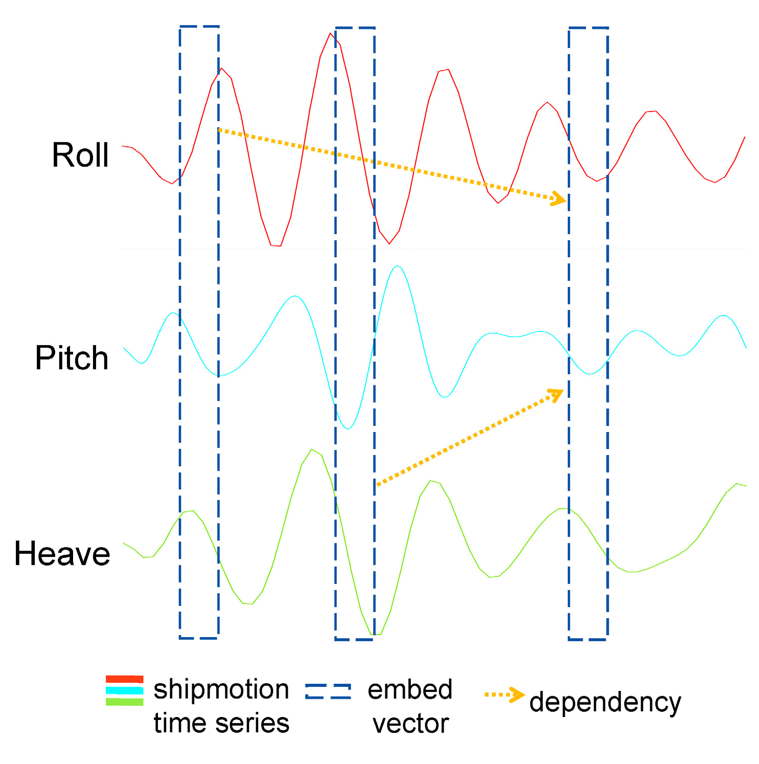
Cross-Attention [20] (CA) is a mechanism that enhances the extraction of specific information by applying weighted attention to different parts of the input sequences. In CA, the representation of one sequence can be adjusted based on the representation of another sequence, allowing the model to better capture relationships between different modalities or sequences. The advantage of CA lies in its ability to effectively integrate information from different sources [21], making it suitable for tasks such as multimodel learning and machine translation. In time series feature extraction, CA can be used to combine time series data with external information (such as historical data), thereby improving prediction accuracy. By focusing on features related to the target task, CA helps extract valuable latent information, making the model more flexible and accurate when handling complex time series. The mechanism of CA is shown in Figure 1.

This study explores Cross-Attention (CA) in neural networks and attempts to develop new forms of attention to improve model adaptability to complex sea states and ship motion series, aiming to achieve higher predictive accuracy and ensure model robustness.

2. Research Methods

Improving the real-time prediction accuracy of sea state parameters is crucial for maritime operations. During navigation, ships are subjected to six degrees of motion: roll, pitch, yaw, heave, sway, and surge. Previous studies have shown that focusing on roll, pitch, and heave provides sufficient data for predicting sea state parameters while ensuring relatively high computational efficiency.

Due to the simplicity and ease of modification of the model structure, the networks used in this study are derived from those in (Mak and Duz [7], 2019). To improve training efficiency, the two-dimensional convolution layers were replaced by one-dimensional convolutions, and residual connections were introduced to enhance model depth and performance. Additionally, Cross-Attention (CA) was adapted with residual connections and multi-head mechanisms, resulting in Residual Cross-Attention (ResCA), which boosts inter-sequence dependency modeling, parameter efficiency, gradient stability, and overall model performance [22,23].

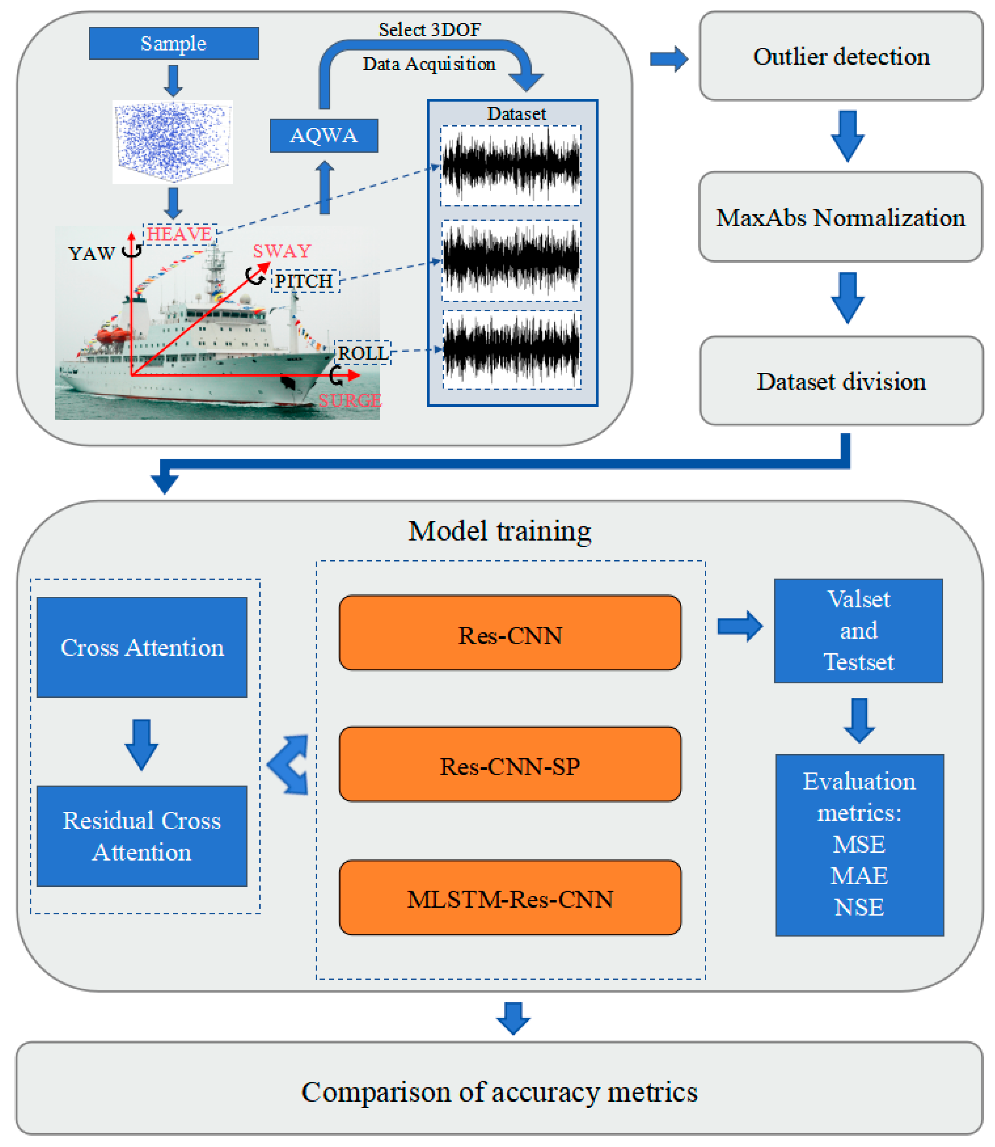
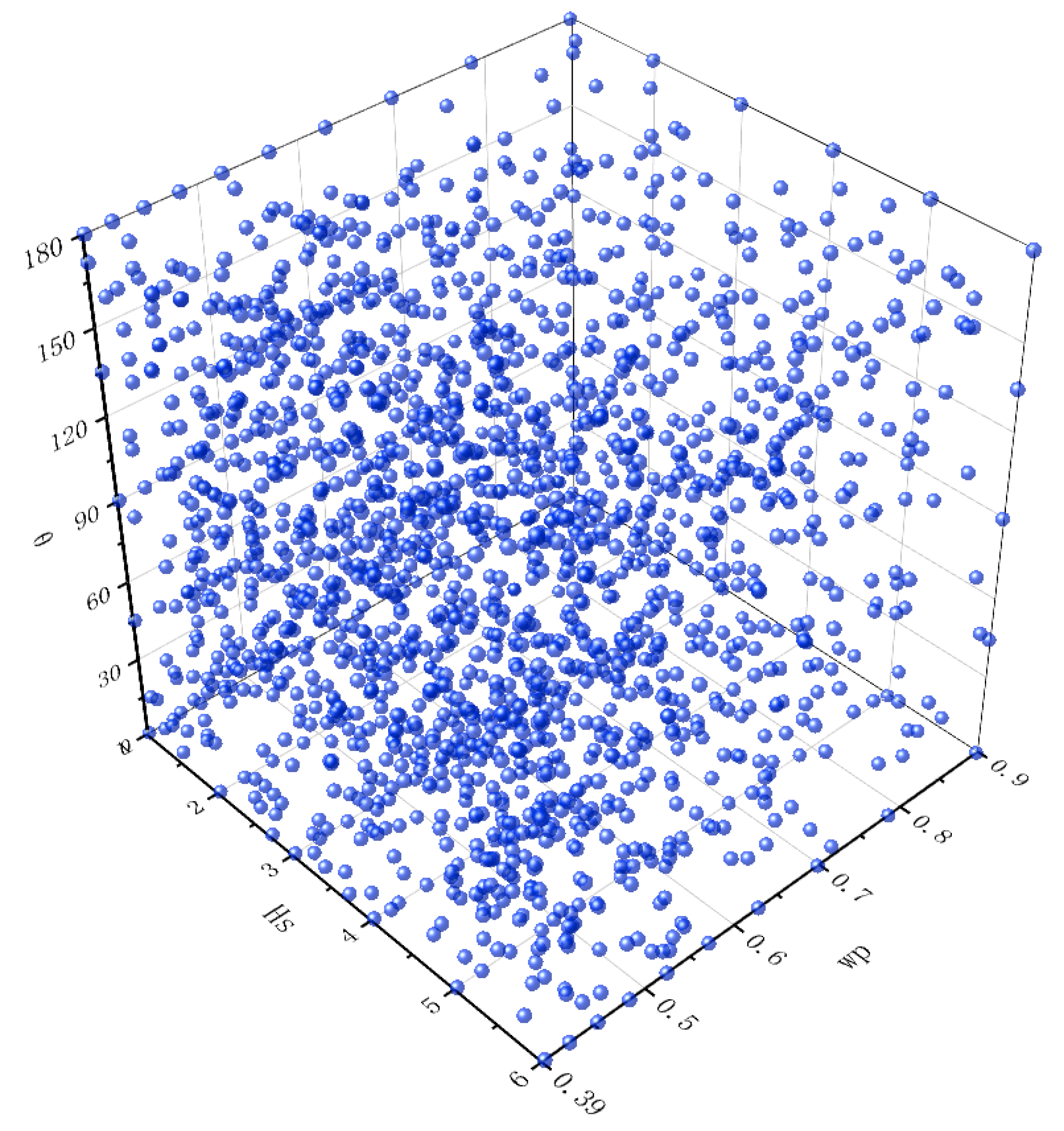
A database of three-degrees-of-freedom response time series for research vessel “Yu kun” under wave influence was constructed. The CA mechanism was adapted, and Res-CNN, Res-CNN-SP, and MLSTM-Res-CNN were used as benchmark models with CA and ResCA introduced, respectively. This approach validated the effectiveness of these mechanisms for sea state parameter prediction and assessed the improvement in prediction accuracy, providing an optimized approach for real-time sea state forecasting in the future. The workflow of this study is shown in Figure 2.

2.1. Res-CNN

The convolution module (Conv-Module), consisting of 1D convolution layers, batch normalization, and ReLU activation functions, is shown in Figure 3. The modular structure facilitates network performance testing and maintenance. This study employs three convolution blocks. The first block contains two convolution modules to reduce data dimensionality. The second block consists of three convolution modules with the same filter numbers, connecting the output of the first convolution block, thereby increasing network depth and alleviating the vanishing gradient problem [24], which is why it is referred to as a residual block. The presence of residual blocks allows for increased depth without significantly raising training difficulty [25]. The third convolution block is used to learn more complex features (such as edges) and reduce the number of channels. Testing indicates that combining a convolution module with an attention module in this block results in the most stable performance.

Adaptive average pooling (AAP) computes the average value within each pooling window to capture global trend information, making it suitable for smooth predictions in regression tasks [26]. So, after the first and third convolution blocks, AAP layers are added, which are more flexible than max pooling and help reduce noise and unnecessary information in the input features. After the final convolution block, a fully connected (FC) layer and a ReLU activation function are added. Finally another FC layer was used to output the results. The Res-CNN network structure is shown in Figure 4.

In the Res-CNN, there are 2, 3, and 1 conv-modules in the first, second, and third convolutional blocks, respectively, with all convolutional layers using 3 kernels. The first block contains 256 and 128 filters in its two modules, while the second block has 128 filters in each of its three modules, maintaining consistency with the output of the first block. The third block includes a single module with 64 filters. Following the convolutional blocks, the FC layers consists of 64 and 3 neurons, with the final layer outputting the predicted sea state parameters.

2.2. Res-CNN-SP

Building on Res-CNN, Res-CNN-SP incorporates the Squeeze and Excitation Block (SEB) and a hybrid pooling structure. The convolutional structure of Res-CNN-SP is the same as that of Res-CNN, consisting of three convolutional blocks. However, Res-CNN-SP replaces the AAP with the SEB, which was set after convolutional layers. The SEB helps suppress irrelevant features and enhances the model’s sensitivity to important features. After the convolution structure, max pooling, min pooling, and average pooling layers are connected, with pooling kernel sizes all set to 1. The fully connected section consists of two FC layers and ReLU activation functions. The network structure of Res-CNN-SP is shown in Figure 5.

The Res-CNN-SP network employs the same parameter configuration as the Res-CNN architecture, with the only difference being that the kernel size of all three pooling layers is set to 1.

2.3. MLSTM-Res-CNN

It is worth mentioning that MLSTM-CNN is a highly promising network architecture; the “parallel formation” was widely used in the task of sea state parameters prediction. In this study, the MLSTM-Res-CNN retains the convolution structure of Res-CNN, with the LSTM layer and convolution structure running in parallel. The LSTM layer is responsible for extracting global temporal dependencies. After combining the results of both, the concatenation is passed through an FC layer to output the final results. The network structure of MLSTM-Res-CNN is shown in Figure 6.

The MLSTM-Res-CNN architecture adopts the same convolutional structure parameters as the previous two networks. Additionally, it includes an LSTM layer with 128 neurons. The output is generated through a single fully connected layer with 3 neurons, corresponding to the predicted sea state parameters.

2.4. Residual Cross-Attention Mechanism

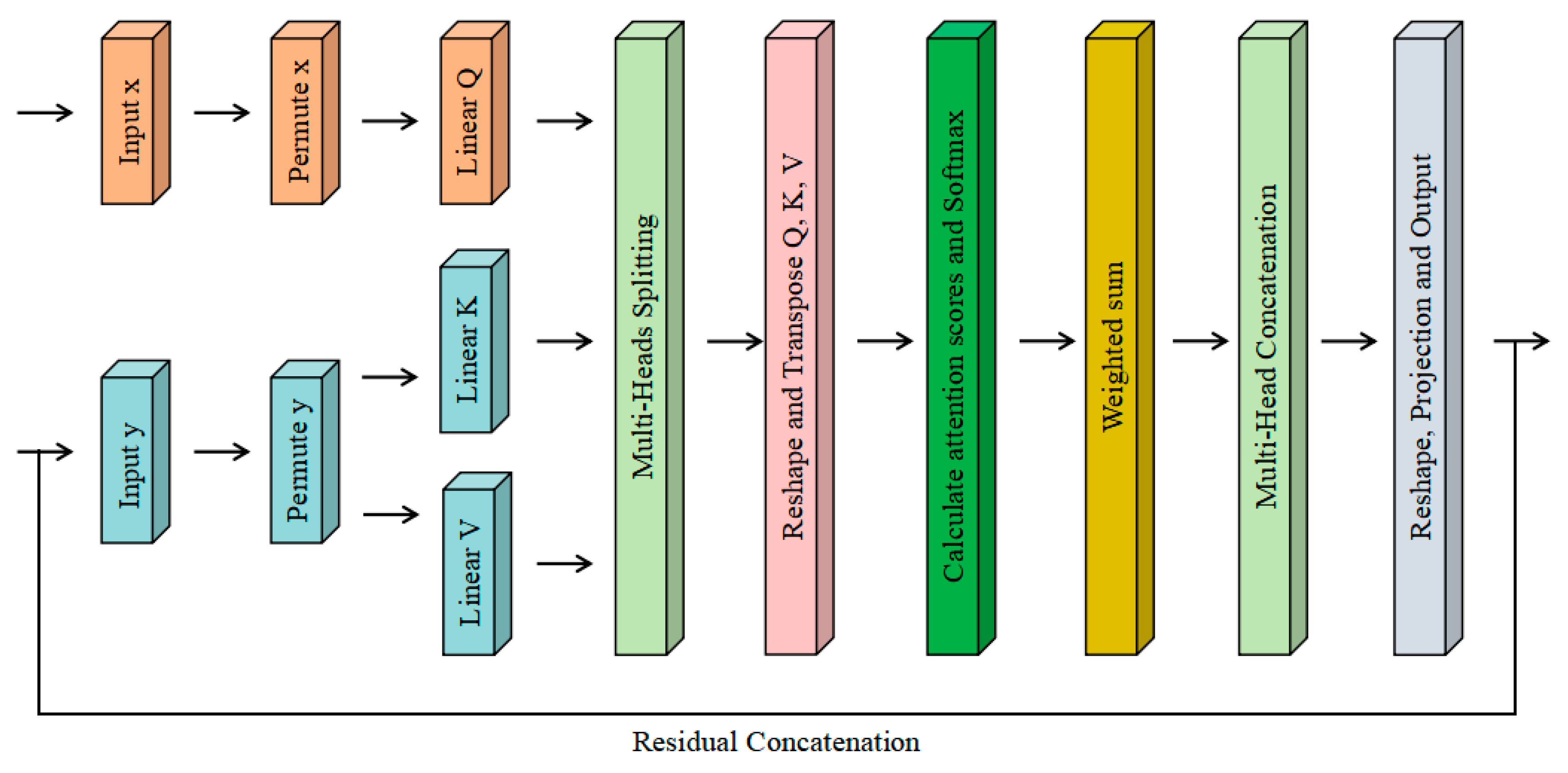
In this work, a Residual Cross-Attention (ResCA) mechanism based on the mathematical logic of Cross-Attention was developed, which involves the methods of calculating attention scores and multi-head segmentation. The advantage of ResCA lies in its dual mechanism: Cross-Attention is used to dynamically adjust feature weights, and residual connections are employed to improve the training stability of deep networks. This ensures that the model maintains strong generalization ability and accuracy under complex sea conditions.

First, the input tensors x and y are transposed to adjust their shapes for subsequent linear layer processing. Then, each tensor undergoes transformation via its respective linear projection layer, generating the Query (Q), Key (K), and Value (V) representations.

$$Q=W_{q}x, K=W_{k}y ,V=W_{v}y$$

(1)

Here, $W_q$, $W_k$, and $W_v$ are learnable linear projection matrices. This operation aims to map the input features into different subspaces to capture finer feature relationships in the attention calculations. Due to the requirement in subsequent operations of the Cross-Attention mechanism that $x$ and $y$ have the same number of channels, the network structure used in this study, which incorporates residual blocks, is particularly well-suited for this characteristic. Therefore, the output of the first convolutional block and the input of the third convolutional block were, respectively, selected as $x$ and $y$.

The generated Q, K, and V tensors are reshaped and divided into multiple groups based on the number of attention heads. Attention head is a parallel computational unit that efficiently extracts various features and relationships from input data, serving as a key component of the attention mechanism [27]. Each group represents a subspace, allowing each attention head to focus on features from different subspaces in parallel. Next, attention scores are calculated by performing matrix multiplication on Q and K, followed by scaling the scores to maintain numerical stability.

$$S={\displaystyle \frac{Q K^T}{\sqrt{d_k}}}+B$$

(2)

Here, $d_k$ represents the dimensionality of the Key, used for scaling to maintain numerical stability, and B is the attention bias. Attention bias is a learnable parameter used to adjust attention scores, enabling the incorporation of prior knowledge or contextual information to enhance model performance. By including B in the formula, the model gains greater flexibility in controlling its focus on different positions or features within the input sequence. This score matrix represents the correlation between the Query and the Key.

Next, the attention scores are normalized using the Softmax function, which converts the scores into a probability distribution to emphasize the relative importance of different inputs, suppress numerical instability caused by large score ranges, and ensure the sum of all attention weights equals 1, generating attention weights between each Q and all K. These weights reflect the relevance between Q and K. Finally, these weights are applied to the V through weighted summation to obtain the output of each attention head. The outputs from all attention heads are then concatenated along the channel dimension and processed through a linear projection layer to produce the output, which is reshaped to match the initial input format before being passed to subsequent modules.

Finally, if the input is added to the output, it is referred to as ResCA, otherwise, it is referred to as CA. The ResCA structure is shown in Figure 7.

$$A=Softmax\left(S\right), Attention=A V$$

(3)

$$Out=Proj\left(Attention\right)+y$$

(4)

Figure 7. Residual Cross-Attention mechanism (ResCA).

Figure 7. Residual Cross-Attention mechanism (ResCA).

3. Dataset Construction and Setup

3.1. Dataset Construction

The selected ship type for this study is the “Yu kun”, with parameters listed in

Table 1. Parameters of the “Yukun”.

Parameter	Value
Lpp	105 m
Breadth	18 m
Draft	5.4 m
Displacement	5878.8 t
Rxx	6.3 m
Ryy	26.25 m
Rzz	26.25 m

, and a 3D model shown in Figure 8. To better simulate real sea conditions, the JONSWAP spectrum was chosen, with the average value of spectral peak correction factor (γ) set to 3.3. A total of 6000 short-crested wave simulations were conducted using random uniform sampling, with the significant wave height (Hs) uniformly distributed in the range of [1 m, 6 m], the peak spectral frequency (${\mathsf{\omega }}_{\mathrm{p}}$) in the range of [0.39 rad/s, 0.90 rad/s], the relative direction (θ) in the range of [0°, 180°], and the spreading factor uniformly distributed in the range of [1, 35]. The sea state scatter plot is shown in Figure 9. The boundary element software was used to calculate the six degrees of freedom of ship motion responses under various sea conditions, with a time step of 0.1 s and a total simulation time of 3600 s. Finally, roll, pitch, and heave were retained to construct the database.

3.2. Training Setting

The operating system used in this study is Windows, with a GPU of 12GB GeForce RTX 3080Ti, CUDA 12.6, and the environment set up through Anaconda. The programming language is Python 3.9, and the model training framework is based on PyTorch 2.4.1.

For data processing, the dataset was divided into training, validation, and test sets, the proportion was 8:1:1, with the number of samples in the validation and test sets being the same. The same validation and test sets were used to evaluate the performance of each model on each task to ensure objectivity in comparisons. The dataset was standardized using the MaxAbs method, scaling the data to the range of [$\frac{min}{max},1$].

The sample batch size was set to 300, with an initial learning rate of 0.0005 and a learning rate decay coefficient of 0.995 to prevent overfitting. The maximum number of training epochs was set to 200, with early stopping configured such that training would stop if the loss did not decrease within 15 epochs. Since this study aims to predict multiple sea condition parameters simultaneously, mean squared error (MSE) was chosen as the loss function based on other research [28]. The optimizer used was Adam and parameters (such as betas, epsilon, and Weight decay) were default.

The hyperparameter values were selected using the Grid Search method [29]. Specifically, for each hyperparameter (such as learning rate, batch size, number of layers, etc.), we defined an empirical search range and conducted a comprehensive exploration of all possible combinations. Hyperparameter tuning was directly performed on the validation set of each ORG scheme. This approach ensured the robustness of the results while reducing computational complexity. The search range of hyperparameters is shown in

Table 2. Search range of hyperparameters.

Learning Rate	Filters #1	Kernel #1	Filters #2	Kernel #2	Filters #3	Kernel #3	Pooling Kernel	LSTM Neurons	FC Neurons
0.001	256, 128	3, 3	128, 128, 128	3, 3, 3	64	3	3, 3, 3	128	64
0.0005	256, 64	1, 1	64, 64, 64	1, 1, 1	32	1	1, 1, 1	64	32
0.0001	256, 32	-	32, 32, 32	-	-	-	-	32	16

.

Each set of experiments, including the three scenarios of no Cross-Attention, Cross-Attention, and Residual Cross-Attention, is conducted with the same hyperparameters, dataset, and measurement standards for training and evaluation. The only difference lies in whether or not the attention module is introduced. All variations in error are solely attributed to the effect of introducing attention, rather than other factors such as the dataset or measurement errors. So, using the same set of hyperparameters for the CA and ResCA schemes as those applied to the ORG scheme does not imply that this set represents the optimal hyperparameter configuration for the CA and ResCA schemes. The hyperparameter combinations used in the networks are shown in

Table 3. Hyperparameter setting.

	Conv Block #1		Conv Block #2		Conv Block #3		Fully Connected	Others
	Filters	Kernel	Filters	Kernel	Filters	Kernel	Neurons	Pooling Kernel	LSTM Neurons
Res-CNN	256, 128	3,3	128, 128, 128	3, 3, 3	64	3	64	-	-
Res-CNN-SP	256, 128	3,3	128, 128, 128	3, 3, 3	64	3	32	1, 1, 1	-
MLSTM-Res-CNN	256, 128	3,3	128, 128, 128	3, 3, 3	64	3	64	-	128

. Moreover, the number of attention heads was set to 1/64 of the channels.

4. Result and Discussion

To evaluate the prediction performance of the neural network model, various objective evaluation metrics are commonly used. In this study, Mean Squared Error (MSE), Mean Absolute Error (MAE), and Nash–Sutcliffe Efficiency (NSE) are adopted for comparison, with the calculation formulas shown in Equations (5)–(7). Generally, the lower the MSE and MAE, and the higher the NSE, the better the model’s predictive performance. MSE is more sensitive to outliers, while MAE reflects the overall bias. NSE is suitable for large datasets and can indicate the overall fitting performance of the model.

$$\mathrm{M}\mathrm{S}\mathrm{E}={\displaystyle \frac{1}{\mathrm{n}}}\sum _{\mathrm{i}=1}^{\mathrm{n}}{(y_i-{\widehat{y}}_i)}^2$$

(5)

$$\mathrm{M}\mathrm{A}\mathrm{E}={\displaystyle \frac{1}{\mathrm{n}}}\sum _{\mathrm{i}=1}^{\mathrm{n}}\left|y_i-{\widehat{y}}_i\right|$$

(6)

$$\mathrm{N}\mathrm{S}\mathrm{E}=1-{\displaystyle \frac{\sum _{\mathrm{i}=1}^{\mathrm{n}}{(y_i-{\widehat{y}}_i)}^2}{\sum _{\mathrm{i}=1}^{\mathrm{n}}{(y_i-\overline{y})}^2}}$$

(7)

In the above equations, ${\mathrm{y}}_{\mathrm{i}}$ is the predicted value, ${\widehat{\mathrm{y}}}_{\mathrm{i}}$ is the true value, and $\overline{y}$ is the mean of the true values.

The experiment focuses on three scenarios: without embedding any module, embedding Cross-Attention (CA), and embedding Residual Cross-Attention (ResCA). During the experiment, no hyperparameters or network parameters were modified to ensure an intuitive presentation of the model’s performance after embedding the modules. The model performance evaluation metrics are shown in

Table 4. Model evaluation metrics.

			Validation Set			Test Set
			MSE	MAE	NSE	MSE	MAE	NSE
Res-CNN	ORG	Hs	0.001147	0.024388	0.984397	0.001024	0.025192	0.985889
		${\omega }_p$	0.001064	0.022875	0.959172	0.001189	0.024909	0.956673
		θ	0.002949	0.036272	0.971027	0.002478	0.035253	0.976471
	CA	Hs	0.001013	0.023709	0.986222	0.000969	0.023296	0.986651
		${\omega }_p$	0.000838	0.018987	0.967840	0.000866	0.018815	0.968424
		θ	0.002457	0.031779	0.975856	0.001841	0.027402	0.982523
	ResCA	Hs	0.000998	0.017185	0.986419	0.000498	0.015254	0.993139
		${\omega }_p$	0.000613	0.017450	0.976480	0.000666	0.017533	0.975725
		θ	0.002586	0.033266	0.974585	0.002219	0.031787	0.978938
Res-CNN-SP	ORG	Hs	0.0027043	0.0439817	0.9632147	0.0025498	0.0433486	0.9648637
		${\omega }_p$	0.0009465	0.0213340	0.9636925	0.0010490	0.0221563	0.9617663
		θ	0.0036346	0.0372082	0.9642848	0.0024986	0.0351724	0.9762800
	CA	Hs	0.0008791	0.0211957	0.9880420	0.0008614	0.0210325	0.9881294
		${\omega }_p$	0.0007378	0.0186352	0.9716958	0.0006282	0.0174561	0.9771042
		θ	0.0019410	0.0266659	0.9809274	0.0014964	0.0233526	0.9857937
	ResCA	Hs	0.0009329	0.0208743	0.9873102	0.0007115	0.0190380	0.9901957
		${\omega }_p$	0.0002733	0.0122951	0.9895169	0.0005040	0.0141176	0.9816315
		θ	0.0022446	0.0210007	0.9779441	0.0007860	0.0171486	0.9925379
MLSTM-Res-CNN	ORG	Hs	0.0015612	0.0305452	0.9787639	0.0013109	0.0296474	0.9819360
		${\omega }_p$	0.0006624	0.0166935	0.9745906	0.0007141	0.0178950	0.9739744
		θ	0.0046528	0.0469557	0.9542796	0.0033330	0.0456188	0.9683583
	CA	Hs	0.0008174	0.0171347	0.9888812	0.0005492	0.0169147	0.9924327
		${\omega }_p$	0.0005387	0.0136950	0.9793363	0.0004056	0.0124306	0.9852184
		θ	0.0023382	0.0323791	0.9770242	0.0017678	0.0306845	0.9832175
	ResCA	Hs	0.0006889	0.0183671	0.9906299	0.0005634	0.0175631	0.9922358
		${\omega }_p$	0.0003512	0.0122083	0.9865274	0.0004732	0.0133149	0.9827524
		θ	0.0018800	0.0214926	0.9815260	0.0011698	0.0209302	0.9888941

.

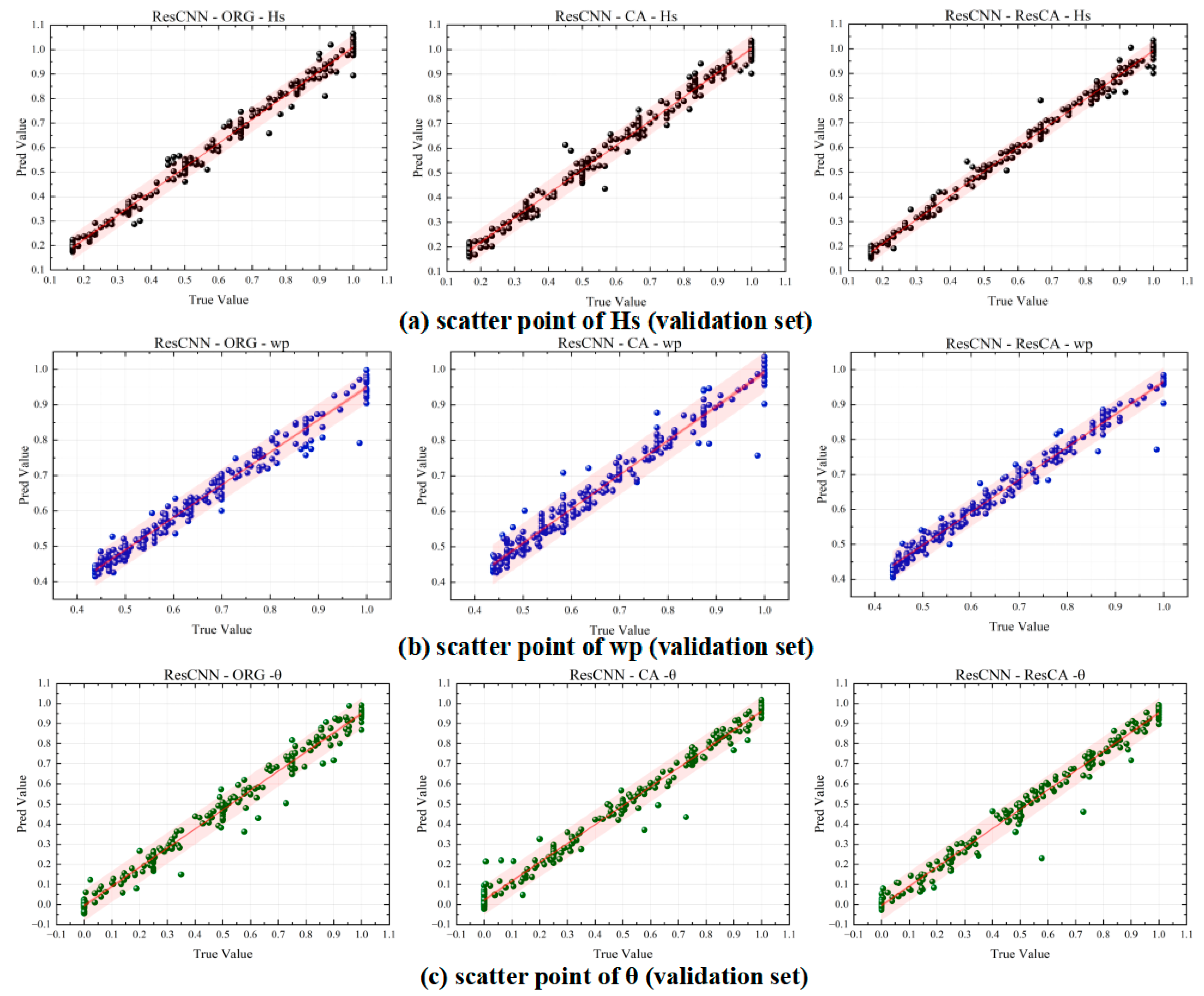
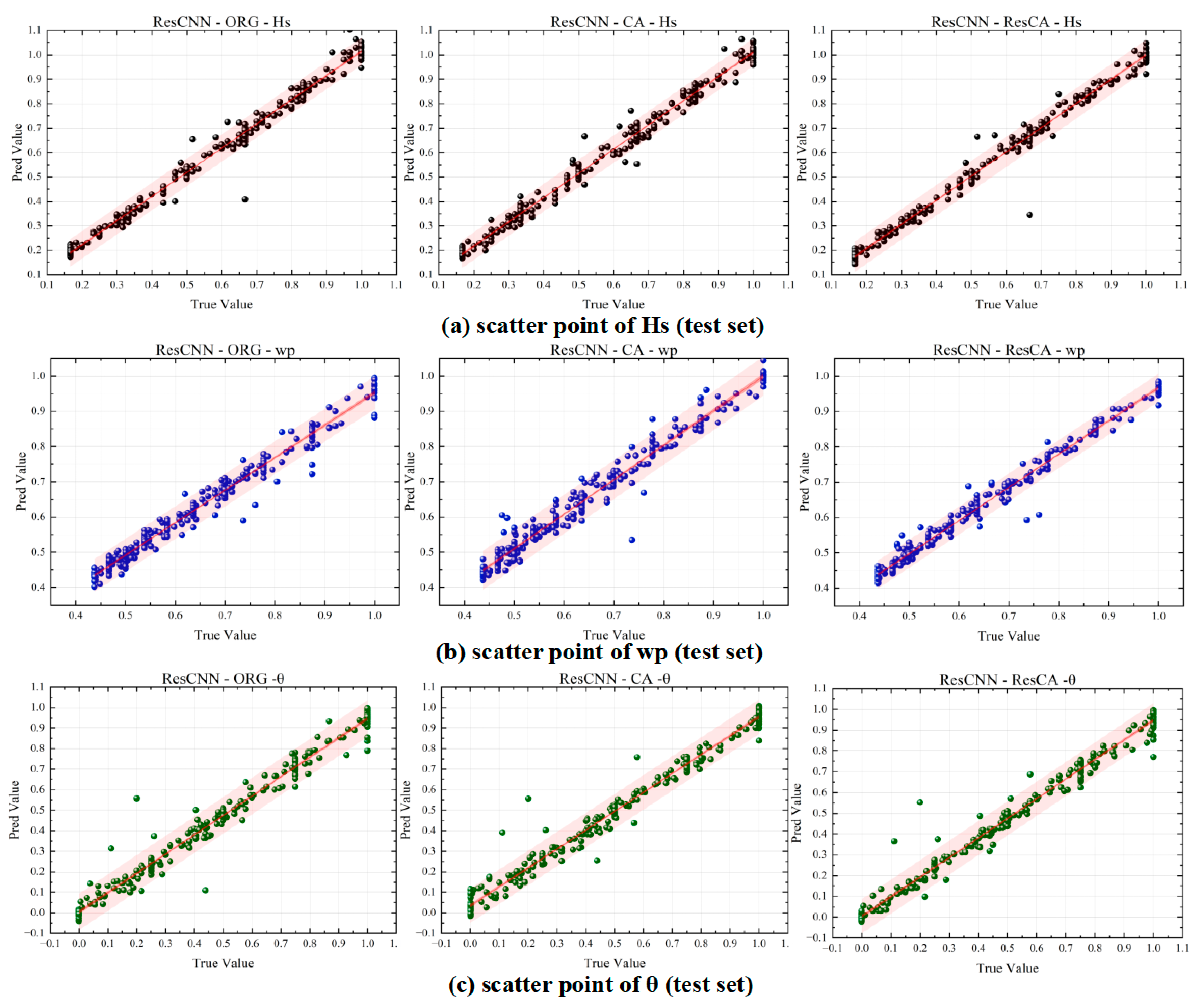
To facilitate the comparison of prediction results, after completing the training and making predictions on both the validation and test sets, the predicted values were not inverse normalized, meaning the dimensionless quantities were directly compared. The ranges for significant wave height (Hs), peak frequency (${\mathsf{\omega }}_{\mathrm{p}}$), and relative direction (θ) were scaled to [0.167, 1], [0.433, 1], and [0, 1], respectively. The scatter plots for the validation and test sets are shown in Figure 10 and Figure 11. The rows in the figures represent tasks for Hs, ${\mathsf{\omega }}_{\mathrm{p}}$, and θ, while the columns represent the following methods: the ORG scheme (no attention), the CA scheme (Cross-Attention), and the ResCA scheme (Residual Cross-Attention).

On the validation set, the Res-CNN-CA scheme showed a narrower light red prediction interval compared to Res-CNN-ORG, with the scatter points more concentrated near the diagonal, although the dark red confidence interval showed slight change. This indicates that the prediction value is more likely to be close to the true value, meaning the CA module improved feature extraction capabilities and reduced prediction errors. The ResCA scheme further optimized the model performance, and the prediction interval also contracted significantly, with fewer large error points, indicating higher precision and stability.

On the test set, the Res-CNN-CA scheme still outperformed Res-CNN-ORG, with the data points more concentrated near the diagonal, a narrower prediction interval, and reduced errors in the higher value regions, demonstrating that the CA module improved the model’s generalization ability. The ResCA scheme continued to perform best on the test set, with the narrowest confidence and prediction intervals and the least number of large errors, showcasing stronger stability and generalization.

The scatter plot results suggest that the CA module improved prediction accuracy on top of the Res-CNN architecture, while the ResCA module further enhanced the model’s stability and generalization ability. Moreover, similar conclusions can be drawn from the prediction scatter plots of the other two models, and will not be discussed further to avoid redundancy.

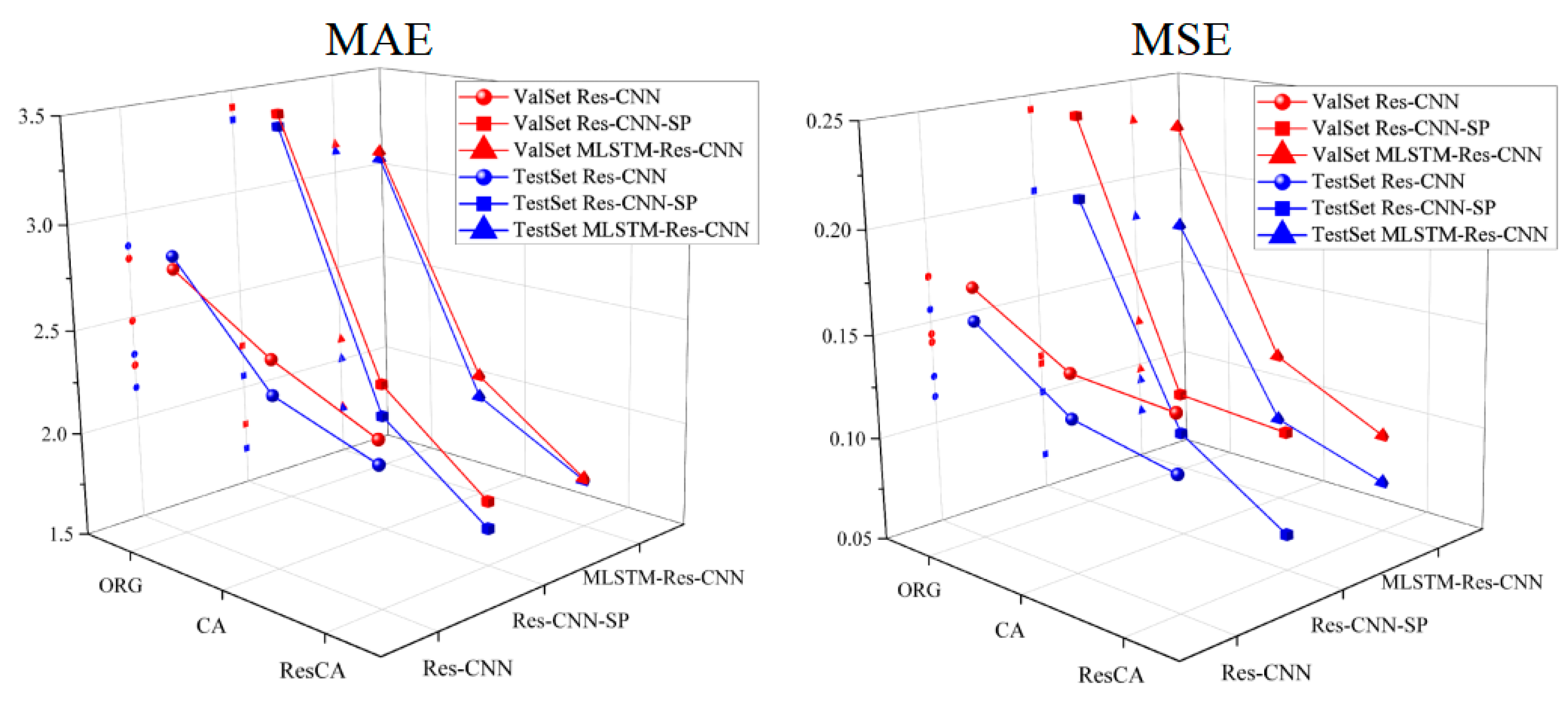
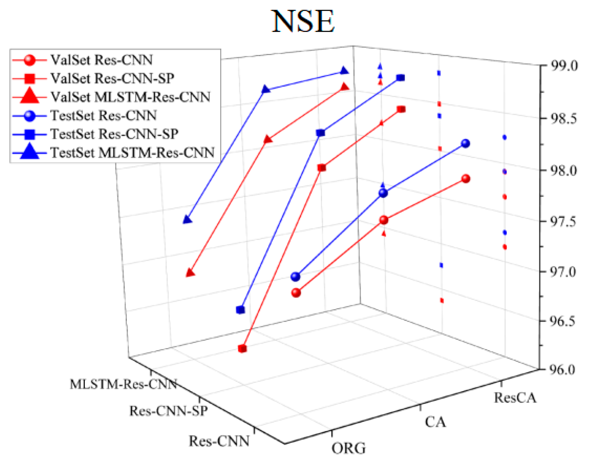
Since the three tasks correspond to several evaluation metrics, to facilitate the discussion on model performance improvement, the average values of various evaluation metrics (MAE, MSE, and NSE) are calculated and analyzed. The changes in the evaluation metrics are shown in Figure 12 and Figure 13.

For MAE, the MAE of the validation set (red line) and test set (blue line) gradually decreased as the modules were improved. Among the three models (Res-CNN, Res-CNN-SP, MLSTM-Res-CNN), the effects of adding the CA and ResCA modules were more significant. The ResCA module significantly reduced the MAE, indicating its superiority in error control compared to the ORG and CA schemes. This further proves that after introducing the ResCA module, the narrowing of the prediction intervals in the scatter plots is due to the model demonstrating stronger stability.

For MSE, the trend in the validation and test sets is similar to that of MAE. After introducing the CA module, the errors noticeably decreased, while the ResCA module further reduced the MSE, showing higher prediction accuracy. The advantage of the ResCA module in MSE is especially prominent, particularly in the Res-CNN-SP and MLSTM-Res-CNN structures. This is consistent with the reduction in large error points in the ResCA scatter plots shown in Figure 11.

For the NSE metric, higher values indicate better model performance. The NSE values of the validation and test sets gradually improved as the model progressed from the ORG to the CA, and finally to the ResCA module. The ResCA module performed best in terms of NSE across all three models, especially in the MLSTM-Res-CNN structure, where it achieved the highest accuracy, as shown in

Table 5. Comprehensive (average) evaluation metrics (×10²).

		Res-CNN			Res-CNN-SP			MLSTM-Res-CNN
		ORG	CA	ResCA	ORG	CA	ResCA	ORG	CA	ResCA
ValSet	MSE	0.1720	0.1436	0.1399	0.2428	0.1186	0.1150	0.2292	0.1231	0.0973
	MAE	2.7845	2.4825	2.2633	3.4175	2.2166	1.8057	3.1398	2.1070	1.7356
	NSE	97.1532	97.6639	97.9161	96.3731	98.0222	98.4924	96.9211	98.1747	98.6228
TestSet	MSE	0.1564	0.1225	0.1128	0.2032	0.0995	0.0667	0.1786	0.0908	0.0735
	MAE	2.8451	2.3171	2.1525	3.3559	2.0614	1.6768	3.1054	2.0010	1.7269
	NSE	97.3011	97.9199	98.2601	96.7637	98.3676	98.8122	97.4756	98.6956	98.7961

.

The projection points in the image also indicate that as the attention scheme changes, the model performance gradually improves.

In addition, as shown in Figure 14, it can be observed that due to the differences between the validation and test sets, the performance of each model on the test set is relatively better. But the position of red and blue points indicates that embedding CA can improve the model’s performance in predicting sea condition parameters to some extent, and embedding ResCA further enhances performance. Furthermore, whether on the validation set or the test set, the neural network with embedded ResCA exhibits superior robustness, showing balanced prediction advantages on both sets. This proves that the network with the embedded ResCA module also has excellent generalization capability. Therefore, it can be concluded that the ResCA module has good applicability.

The evaluation metrics for the CA scheme relative to the ORG scheme, and for the ResCA scheme relative to the CA scheme, across different networks and datasets, are shown in

Table 6. Relative change of evaluation metrics.

		Res-CNN		Res-CNN-SP		MLSTM-Res-CNN
		CA vs. ORG	ResCA vs. CA	CA vs. ORG	ResCA vs. CA	CA vs. ORG	ResCA vs. CA
Valset	MSE	−16.50%	−2.56%	−51.16%	−3.01%	−46.28%	−20.96%
	MAE	−10.85%	−8.83%	−35.14%	−18.54%	−32.90%	−17.63%
	NSE	0.53%	0.26%	1.71%	0.48%	1.29%	0.46%
Testset	MSE	−21.64%	−7.99%	−51.03%	−32.97%	−49.19%	−18.96%
	MAE	−18.56%	−7.11%	−38.57%	−18.66%	−35.56%	−13.70%
	NSE	0.64%	0.35%	1.66%	0.45%	1.25%	0.10%

and Figure 15.

In the comparison of CA scheme vs. ORG scheme, the specific increments for MSE, MAE, and NSE are as follows: both MSE and MAE show negative values, indicating that the CA model significantly reduces the error compared to the original model (ORG scheme). In the validation set, Res-CNN reduced MSE by 16.50%, Res-CNN-SP reduced it by 51.16%, and MLSTM-Res-CNN reduced it by 46.28%. In the test set, Res-CNN reduced MSE by 21.64%, Res-CNN-SP reduced it by 51.03%, and MLSTM-Res-CNN reduced it by 49.19%. These results show that the CA model significantly improves prediction accuracy compared to the original model, especially with a substantial reduction in error in both the validation and test sets. The NSE increments in both the validation and test sets are positive, indicating that the CA model improves prediction consistency and feature capture capability. In the validation set, NSE increased by 0.53% (Res-CNN), 1.71% (Res-CNN-SP), and 1.29% (MLSTM-Res-CNN); in the test set, the increments were 0.64%, 1.66%, and 1.25%, respectively. These positive increments indicate that the CA model has an advantage in terms of explanatory power and prediction consistency over the original model.

In the comparison of the ResCA scheme vs. CA scheme, the increments for MSE, MAE, and NSE are as follows: negative increments for both MSE and MAE reflect that the ResCA model further reduces the error in both the validation and test sets. In the validation set, Res-CNN reduced MSE by 2.56%, Res-CNN-SP reduced it by 3.01%, and MLSTM-Res-CNN reduced it by 20.96%; in the test set, Res-CNN reduced MSE by 7.99%, Res-CNN-SP reduced it by 32.97%, and MLSTM-Res-CNN reduced it by 18.96%. This shows that the ResCA model is particularly effective in the test set, with significant reductions in error. The positive increment in NSE indicates that the ResCA model further improves prediction consistency in both the validation and test sets. In the validation set, NSE increased by 0.26% (Res-CNN), 0.48% (Res-CNN-SP), and 0.46% (MLSTM-Res-CNN); in the test set, the increments were 0.35%, 0.45%, and 0.10%, respectively.

Based on the above comparison analysis, the CA scheme significantly reduces the error when compared to the original scheme (ORG), especially in MSE and MAE, and also shows an improvement in predicting NSE, demonstrating better overall prediction performance. Further, when introducing ResCA, compared to the CA scheme, the error is further reduced, while showing higher prediction consistency in the NSE metric. This indicates that ResCA can further improve prediction accuracy while enhancing the robustness and feature-capturing ability of the model, making it more effective in practical applications.

5. Conclusions

In order to further improve prediction accuracy and ensure the robustness of the model, this study investigates Cross-Attention (CA) based on neural networks and proposes a novel prediction method based on Residual Cross-Attention (ResCA), aimed at enhancing the model’s adaptability to complex sea conditions. This study innovatively introduces the Cross-Attention mechanism into sea state parameters prediction tasks and, based on this mechanism, develops a deep learning method with a Residual Cross-Attention mechanism (ResCA) to improve the prediction accuracy of sea state parameters. Through multi-task learning, the feasibility of embedding the two modules is validated, and the performance of models with no embedding, embedding the Cross-Attention (CA) module, and embedding the Residual Cross-Attention (ResCA) module is compared.

The research results show that models with embedded Cross-Attention (CA) and Residual Cross-Attention (ResCA) significantly outperform the baseline model without attention mechanisms in predicting sea state parameters. Furthermore, embedding ResCA has a significant effect on the model’s robustness and generalization ability, as evidenced by the noticeable improvement in the average absolute error (MAE) and mean squared error (MSE), reflecting higher prediction stability.

Moreover, by embedding ResCA into different baseline networks (Res-CNN, Res-CNN-SP, and MLSTM-Res-CNN), the effectiveness and practicality of this attention mechanism have been verified. This Cross-Attention mechanism that based on residual connection not only improves the overall prediction performance of the model on most samples but also effectively reduces the impact of data points with large prediction errors.

Finally, this study provides a new approach for real-time sea state parameter prediction, where the model can enhance its prediction capability for complex sea conditions without significantly increasing training difficulty by using the ResCA module. This method demonstrates good applicability and provides reliable support for future marine environmental prediction tasks.

However, ResCA is an attention module designed for ship motion in three degrees of freedom (roll, pitch, and heave), and its limitations lie in scenarios with small data dimensions. It is difficult to directly apply it to multimodel and high-dimensional data scenarios (e.g., with the inclusion of mooring forces and other time series features).