Vessel Type Recognition Using a Multi-Graph Fusion Method Integrating Vessel Trajectory Sequence and Dependency Relations

Abstract

In the field of research into vessel type recognition utilizing trajectory data, researchers have primarily concentrated on developing models based on trajectory sequences to extract the relevant information. However, this approach often overlooks the crucial significance of the spatial dependency relationships among trajectory points, posing challenges for comprehensively capturing the intricate features of vessel travel patterns. To address this limitation, our study introduces a novel multi-graph fusion representation method that integrates both trajectory sequences and dependency relationships to optimize the task of vessel type recognition. The proposed method initially extracts the spatiotemporal features and behavioral semantic features from vessel trajectories. By utilizing these behavioral semantic features, the key nodes within the trajectory that exhibit dependencies are identified. Subsequently, graph structures are constructed to represent the intricate dependencies between these nodes and the sequences of trajectory points. These graph structures are then processed through graph convolutional networks (GCNs), which integrate various sources of information within the graphs to obtain behavioral representations of vessel trajectories. Finally, these representations are applied to the task of vessel type recognition for experimental validation. The experimental results indicate that this method significantly enhances vessel type recognition performance when compared to other baseline methods. Additionally, ablation experiments have been conducted to validate the effectiveness of each component of the method. This innovative approach not only delves deeply into the behavioral representations of vessel trajectories but also contributes to advancements in intelligent water traffic control.

1. Introduction

With the rapid development of the global economy, the ocean, as a key channel for global trade, is becoming increasingly significant in maritime situational awareness and maritime supervision. Especially in the context of a substantial increase in the number of vessels and the increasingly complex maritime traffic environment, the introduction of an automatic identification system (AIS) has provided strong technical support, reducing maritime accident rates and enhancing the efficiency of ocean management.

The rapid advancement of information technology, especially the rapid development of the global positioning system (GPS), has greatly enhanced the detail found in AIS data and its application scope. Currently, AIS data provide an indispensable data foundation for fields such as maritime traffic analysis [1], vessel behavior analysis [2], maritime safety supervision [3], and marine pollution detection [4]. However, the accuracy and completeness of AIS data still face many challenges, such as the absence and incorrect labeling of vessel-type information [5], data imbalance, and quality problems [6]. This increases the difficulty of maritime supervision and also highlights the necessity of achieving the accurate recognition of vessel types.

Accurately recognizing vessel types plays a crucial role in enhancing maritime situational awareness [7], maritime surveillance [8], vessel behavior pattern mining [9], and anomaly detection [10]. However, the issue of the accuracy of AIS information is still prominent, especially the potential for non-authentic vessel-type information in AIS messages. This could be due to crew members manually entering incorrect information or intentionally concealing vessel types [11] to engage in illegal activities related to fishing [12] and smuggling [13]. Therefore, inferring vessel types based on their movement trajectories has become an effective method to address this issue and has gradually become a research hotspot. Despite the many achievements in the research of vessel-type recognition, there are still several shortcomings. Firstly, AIS data are used as a time series with irregular sampling and contain location information. Many studies use data smoothing technology during data preprocessing, which may lead to the loss of extreme point information [3,14]. Most of these points are often the feature points of trajectory behavior, affecting the accuracy of recognition results. Secondly, due to the issues of missing and incorrectly filled static data, some studies only rely on the static features of vessels or combine static features with dynamic features for classification [15,16,17]. This may result in incomplete feature extraction and a failure to fully utilize the vessels’ various features, such as semantic behavioral features. Some scholars also use the ability of convolutional networks to extract spatial dependencies and combine convolutional neural networks (CNNs) to model spatial dependencies, to enhance the expressive ability of vessel behavior [18]. However, due to the lack of regular road network information at sea, although some studies have begun to consider the relationships between adjacent points in the extraction trajectory, many methods still focus on representative extraction through the sequence relationship of the trajectory [19,20]. Ignoring the dependence between trajectory points, this technique fails to fully capture the vessel’s driving mode and behavior characteristics. In summary, the current vessel type recognition method is prone to information loss in data preprocessing, incomplete feature extraction, and ignoring the dependence between trajectory points. This leads to insufficient representation of trajectory behavior, which affects the accuracy of vessel type recognition.

In response to the aforementioned issues, this paper proposes a vessel type recognition algorithm based on the fusion representation of graph-embedding vessel trajectory sequence and dependency relationships. Firstly, we utilize the dynamic information of AIS data to extract the spatiotemporal features representing vessel positions and semantic features representing vessel behavior, meeting the needs of subsequent key node extraction and trajectory representation. Secondly, we employ algorithms from information theory to automatically identify key nodes from the vessel’s behavioral semantic features. These key nodes include trajectory behavior feature information, which is necessary for building trajectory dependency. On this basis, the graph theory method is used to establish the trajectory sequence graph and the dependency graph. These can accurately capture the sequence and dependency relationships between the vessel trajectory points, which provide the data basis for the subsequent model representation extraction. Subsequently, we propose a multi-graph fusion representation vessel type recognition model. This model utilizes multi-layer graph convolutional networks (GCN) to efficiently aggregate information from adjacent nodes and key nodes. By extracting the sequential features and dependency features from vessel trajectories, it fuses them into a high-order representation vector containing vessel trajectory behavior information, which is applied to downstream vessel trajectory type recognition tasks. Finally, through comparative experiments with the existing algorithms, we validate that our method not only obtains richer vessel trajectory behavior representations but also enhances the performance of trajectory classification tasks, and the performance is better than other baseline methods.

2. Related Work

At present, significant progress has been made in related research on vessel trajectory type recognition using AIS trajectory data. Early research mainly relied on rule-based classification recognition methods. The basic idea of these methods is to extract the parameters of various category features through expert experience and many experiments and then set the corresponding recognition rules to realize the classification. Specifically, when the matching degree between the features of the target data and the condition of the preset rule exceeds the set threshold, the data are classified into the corresponding category [21]. Although this method is effective in certain specific situations, it requires the setter to have profound professional knowledge, and the process of setting identification rules and thresholds is cumbersome and time-consuming.

As machine learning (ML) technology advances, many studies have used ML algorithms to enhance the accuracy of vessel trajectory classification. The fundamental concept is to construct a classifier using probability and statistical methods to classify and recognize objects from trajectory data [22]. Lang et al. [23] proposed an improved multi-class adaptive support vector machine (SVM) for vessel trajectory classification. By combining synthetic aperture radar (SAR) image analysis with AIS data, they improved the accuracy of vessel classification. Yan et al. [15] proposed a vessel classification and anomaly detection method considering their behavioral features, based on Spaceborne AIS data. By extracting both the static and dynamic features of vessels and utilizing SVM and random forest (RF) techniques, the authors achieved vessel classification. This method not only improved the accuracy of classification but also detected abnormal vessel behavior. To validate the effectiveness of different machine learning algorithms in classification tasks, Huang et al. [16] compared the performance of eight machine learning methods in vessel classification tasks. They found that tree-structure-based algorithms, especially extreme gradient boosting (XGBoost) and RF, performed exceptionally well in terms of classification accuracy. On this basis, scholars have further improved the accuracy of trajectory classification and the stability of the algorithm by integrating machine learning algorithms [24,25]. Additionally, some scholars have used ML algorithms such as the decision tree (DT) algorithm and k-nearest neighbor classification (KNN) for vessel type recognition. Although these methods have made some progress in terms of feature selection and parameter tuning, they still rely on empirical knowledge, requiring multiple adjustments and optimizations to achieve the best performance. More importantly, these methods often ignore the relationships between the spatiotemporal features of the vessel trajectory dataset itself.

Benefiting from the strengths of deep learning (DL) in processing high-dimensional data and its ability to automatically extract features with minimal manual intervention, some DL algorithms are capable of learning advanced feature representations from raw data and exhibit good recognition ability. Yang et al. [17] analyzed vessel trajectory data and utilized CNN for pattern recognition, effectively identifying different types of vessels. Guo and Xie [26] proposed a deep convolutional model based on vessel trajectory classification, converting vessel trajectory data into images and employing an improved residual network (ResNet50) model for vessel trajectory classification. However, while converting trajectory data into two-dimensional planar images is somewhat feasible, such images are not directly applicable to real-world scenarios and struggle to capture the contextual information of position sequences that change over time within the trajectories.

To address this issue, Li et al. [19] proposed a large-scale AIS trajectory vessel classification method based on graph neural networks (GNN). They considered the correlation between the points of the trajectory sequence, preprocessed the vessel trajectory data into graph data, and leveraged the GNN’s ability to aggregate adjacent node information to effectively classify four types of vessels. Additionally, some scholars adopted a recurrent neural network (RNN) architecture. For instance, Kong et al. [20] improved the accuracy of vessel identification by calculating various distances to construct a context information knowledge base and combining it with long short-term memory (LSTM) models, but this method is only suitable for coastal areas. Furthermore, Llerena et al. [27] experimentally evaluated the performance of LSTM and CNN in actual vessel trajectory classification tasks, providing a basis for selecting the most appropriate model.

However, the models that were developed based on trajectory sequences frequently lack a consideration of the dependency relations among trajectory points. To address this issue, Wang et al. [28] proposed a multi-feature ensemble learning classification model (MFELCM), which integrates multiple features such as static, dynamic, and time series, and integrates multiple learning algorithms. The accuracy of vessel classification was improved. Syed and Ahmed [29] further proposed an architecture that combined 1D-CNN and LSTM. They used CNN to extract the spatial features and then used LSTM to process the time series features of vessel trajectories, thereby improving the recognition accuracy of vessel trajectories. Aiming at the problem that the extraction of trajectory features fails to effectively consider the semantic information of the trajectory, Yuan et al. [30] constructed a fishing vessel-type recognition method using semantic feature vectors. They analyzed and extracted the semantic features of fishing vessels and input them into a light gradient-boosting machine (LightGBM) classification model for the classification of fishing boats. This method can accurately recognize and categorize various classes of fishing vessels.

In summary, most of the current research is often limited to mining vessel trajectory features from the overall perspective of trajectory sequence. Although the spatial dependencies between neighboring points are considered superficially, the deep correlations between the remaining points of the whole trajectory are ignored. This incompleteness of feature extraction makes it difficult for models to effectively extract representative information, thereby affecting the accuracy of vessel trajectory type recognition. Vessel trajectory data contains not only those global features that describe the overall movement trends but also local features that have a dependency relationship between trajectory points.

These local features can capture the spatial location relationship of ships and the context information of behavioral semantics more precisely, which is crucial to improving the accuracy of trajectory classification. Therefore, trajectory data could be fused and represented from the two dimensions of the overall sequence relation and the internal dependency relationship at the same time. Obtaining high-order representation vectors by aggregated representation will greatly improve the accuracy of trajectory classification.

3. Methods

This paper proposes a vessel-type recognition method based on the fusion representation of graph-embedding vessel trajectory sequence and dependency relationships. The process is shown in Figure 1. The method can be divided into the following stages. (1) Data preprocessing. The spatiotemporal features and behavioral semantic features of the trajectory are extracted from the cleaned data to meet the subsequent model input requirements. (2) Model building. Firstly, the key nodes with dependencies are identified and extracted by a specific algorithm. Then, based on the graph paradigm, the trajectory data are transformed into trajectory sequence graphs and dependency graphs. These two types of graph structures reveal the sequence and internal dependency relationships of the trajectories from different perspectives. Secondly, a model combining multi-graph representation is built to deeply encode the two types of graph created, and to extract high-order vessel behavior representation with both the trajectory sequence and dependency relationships. This process not only mines the potential information in trajectory data but also provides strong support for subsequent classification tasks. Then, the multilayer perceptron (MLP) model is used to build a classifier, aiming to train the classifier to accurately recognize different types of vessel trajectories. (3) Results analysis. A series of evaluation indicators are used to comprehensively evaluate the final recognition results to verify the accuracy and effectiveness of the method.

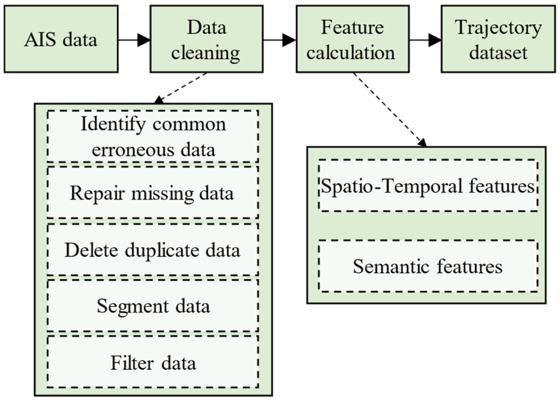
3.1. Data Preprocessing

Data preprocessing involves using the original AIS data to construct a trajectory dataset that meets the input requirements of the subsequent model. This process includes two steps: data cleaning and feature calculation. The specific process is shown in Figure 2. Firstly, through data cleaning work, we remove unnecessary information to improve the reliability and consistency of the data. Secondly, the spatiotemporal features and semantic features of the vessel trajectory are obtained. These features of the information can not only aid in a more comprehensive understanding of the navigational behaviors of vessels but also increase the effectiveness and utilization rate of the data.

3.1.1. Data Cleaning

The original AIS data have many items of static and dynamic attribute information on vessel trajectory, such as MMSI, vessel type, speed over ground (SOG), course over ground (COG), latitude (LAT), and longitude (LON) coordinates. However, due to various factors in the data collection process, the obtained data are often accompanied by errors and abnormal information. Data cleaning was performed before the experiment to meet data quality standards and the subsequent requirements. Therefore, this method conducts data, based on the following criteria:

• Identifying common erroneous data. We check and correct data attribute values that do not conform to common sense rules. For instance, MMSI numbers that are not nine digits, $\left|\mathrm{LAT}\right|>90°$, $\left|\mathrm{SOG}\right|>0kn$, and $\left|\mathrm{COG}\right|\ge 360°$, are all corrected.
• Repairing missing data. Since this study primarily relies on dynamic attribute information within vessel trajectories to infer vessel types, no processing was conducted on static attribute data. To address the issue of missing dynamic attributes, such as LAN, LON, SOG, and COG, we have employed cubic spline interpolation for data imputation to ensure data completeness [31,32].
• Deleting duplicate data. By comparing timestamps and coordinate information, the repeated trajectory points are identified and deleted to reduce data redundancy.
• Segmenting data. The original data is grouped by MMSI number, and then the trajectory data for the same vessel is sorted in chronological order. To address the discontinuity of AIS data, a time threshold of 1800 s is set based on expert experience. Trajectories are segmented using the time threshold method to reduce the impact of data discontinuity in subsequent analyses.
• Filtering data. To optimize the execution efficiency of the model, trajectory segments that contain at least 20 data points are selected. These segments can adequately reflect the characteristics of the vessel’s voyage, while others are discarded due to insufficient information.

3.1.2. Feature Calculation

The dynamic information of vessel trajectories mainly includes the time, LAN, LON, SOG, and COG of trajectory points. Based on the adjacency information found between nodes, GCN can encode the spatial position information and dependency relations between trajectory points to capture the correlations between trajectory points. To more accurately capture the correlations between vessel trajectory points and enhance the model’s recognition capabilities, we introduced finer-grained features. Specifically, based on LAN, LON, and the timestamps of trajectory points, we calculated the time difference $\Delta \mathrm{T}$, longitude difference $\Delta \mathrm{LON}$, latitude difference $\Delta \mathrm{LAT}$, and distance difference $d$. The LAN, LON, $\Delta \mathrm{LAT}$, $\Delta \mathrm{LON}$, $\Delta \mathrm{T}$, and $d$ of each trajectory point were used as the spatiotemporal feature of the vessel trajectory. The specific calculation formulas are as follows:

$$\left\{\begin{array}{c}\Delta \mathrm{T}=\left|{\mathrm{T}}_2-{\mathrm{T}}_1\right|\\ \Delta \mathrm{LAT}=\left|{\mathrm{LAT}}_2-{\mathrm{LAT}}_1\right|\\ \Delta \mathrm{LON}=\left|{\mathrm{LON}}_2-{\mathrm{LON}}_1\right|\\ d=2r\times {\sin }^{-1}\sqrt{{\left(\sin {\displaystyle \frac{\Delta \mathrm{LAT}}{2}}\right)}^2+\cos {\mathrm{LAT}}_1\times \cos {\mathrm{LAT}}_2{\left(\sin {\displaystyle \frac{\Delta \mathrm{LON}}{2}}\right)}^2}\end{array}\right.$$

(1)

where $r=6371.009km$, which is the Earth’s radius.

In addition to the basic spatiotemporal features, we also considered deeper semantic features to provide a more profound understanding of vessel behavior, facilitating the revelation of its inherent patterns and movement rules. Therefore, based on SOG and COG, we calculated $\Delta \mathrm{COG}$ and $\Delta \mathrm{SOG}$. Furthermore, the calculations of acceleration $a$ and angular velocity $\omega$ reflect the vessel’s movement trends and maneuvering capabilities, which are crucial for distinguishing between different types of vessels. We used COG, SOG, $\Delta \mathrm{COG}$, $\Delta \mathrm{SOG}$, $a$, and $\omega$ as semantic features. The specific calculation formulas are as follows.

$$\left\{\begin{array}{c}\Delta \mathrm{COG}={\mathrm{COG}}_2-{\mathrm{COG}}_1\\ \Delta \mathrm{SOG}={\mathrm{SOG}}_2-{\mathrm{SOG}}_1\\ a=\Delta \mathrm{SOG}/\Delta \mathrm{T}\\ \omega =\Delta \mathrm{COG}/\Delta \mathrm{T}\end{array}\right.$$

(2)

In summary, we constructed a 12-dimensional feature vector for each trajectory point. The first six dimensions, $\mathrm{LAT}, \mathrm{LON}, \Delta \mathrm{LAT}, \Delta \mathrm{LON}, \Delta \mathrm{T}, d$, serve as the spatiotemporal feature representation of the trajectory point, while the last six dimensions, $\mathrm{COG}, \mathrm{SOG}, \Delta \mathrm{COG}, \Delta \mathrm{SOG}, a, \omega$, represent the semantic features. This feature vector not only expresses the direct attributes of the trajectory point but also contains information about the correlations between trajectory points, providing strong support for subsequent model training and vessel type recognition.

3.2. Graph Construction for Vessel Trajectories

Based on the extraction of spatiotemporal and semantic features from vessel trajectory data, this study utilizes a graph structure paradigm to represent the trajectories from two aspects, the sequential relationship and the dependency relationship, by constructing a sequence graph and dependency graph. The specific process is shown in Figure 3.

3.2.1. Construction Sequence Graph

Vessel trajectory data essentially form a two-dimensional time series that includes positional attribute information. The trajectory points of each segment are arranged in chronological order, and this sequential characteristic can reflect the adjacency relations between trajectory points. Therefore, a sequence graph is constructed for the trajectory by considering the sequential relationship between the trajectory points. The sequence graph $G_s=\left(V_s,E_s,A_s\right)$ is composed of nodes representing trajectory points and edges, indicating the sequential relationships between adjacent trajectory points. In this graph, the node set $V_s=\left\{v_1,\cdots ,v_n\right\}$ represents the trajectory points, where the nodes $v_i$ and $v_{i+1}$ are adjacent to each other; the sequential relationship is denoted as $R_{seq}\in V_s\times V_s$, and the connections between nodes are represented by $re{l}_{i,i+1}\in R_{seq}$.

3.2.2. Construction Dependency Graph

In constructing the sequence graph, the primary focus is on the sequential relationship between adjacent trajectory points. These sequence points capture the chronological order of the trajectory. However, in contrast, key points are identified, based on specific features of the trajectory, such as turning points or significant changes in direction, and these are not necessarily adjacent. While the sequence graph captures the order of trajectory points in time, it is the semantic dependency relationship between non-adjacent trajectory points, often represented by key points, that provides deeper insights into the vessel’s navigational behavior, such as the identification of navigational patterns or decision-making points along the route.

Therefore, in addition to considering the sequential relation between adjacent trajectory points within each segment, the semantic dependency relationship between non-adjacent trajectory points can provide additional insights into the navigational behavior of the vessel. We represent the dependency relationship between trajectory points as $R_{dep}\in V_d\times V_d$, where the nodes $v_i$ and $v_j$ are connected through the edge relationship $re{l}_{i,j}\in R_{dep}$ shown in the graph. We employ a dependency graph of $G_s=\left(V_d,E_d,A_d\right)$ to describe the nodes in the trajectory and their interrelatedness.

Thus, we achieve the sequence graph $G_s=\left(V_s,E_s,A_s\right)$ and the dependency graph $G_s=\left(V_d,E_d,A_d\right)$. $N$ is the number of trajectory points, $V_s$ and $V_d$ represent the graph node sets, $E_s$ and $E_d$ represent the connecting edges, and $A_s$ and $A_d$ represent the adjacency matrices. We know that the graph nodes in $V_s$ are each point of the trajectory, and the sequential relationship $R_{seq}$ connects adjacent trajectory points through the edges $E_s$. In the dependency graph, the dependency relationship $R_{dep}$ connects trajectory points that exhibit dependency through edges $E_d$. The graph nodes in $V_d$ need to be obtained through algorithmic computation to derive a series of key feature points, which serve as the nodes.

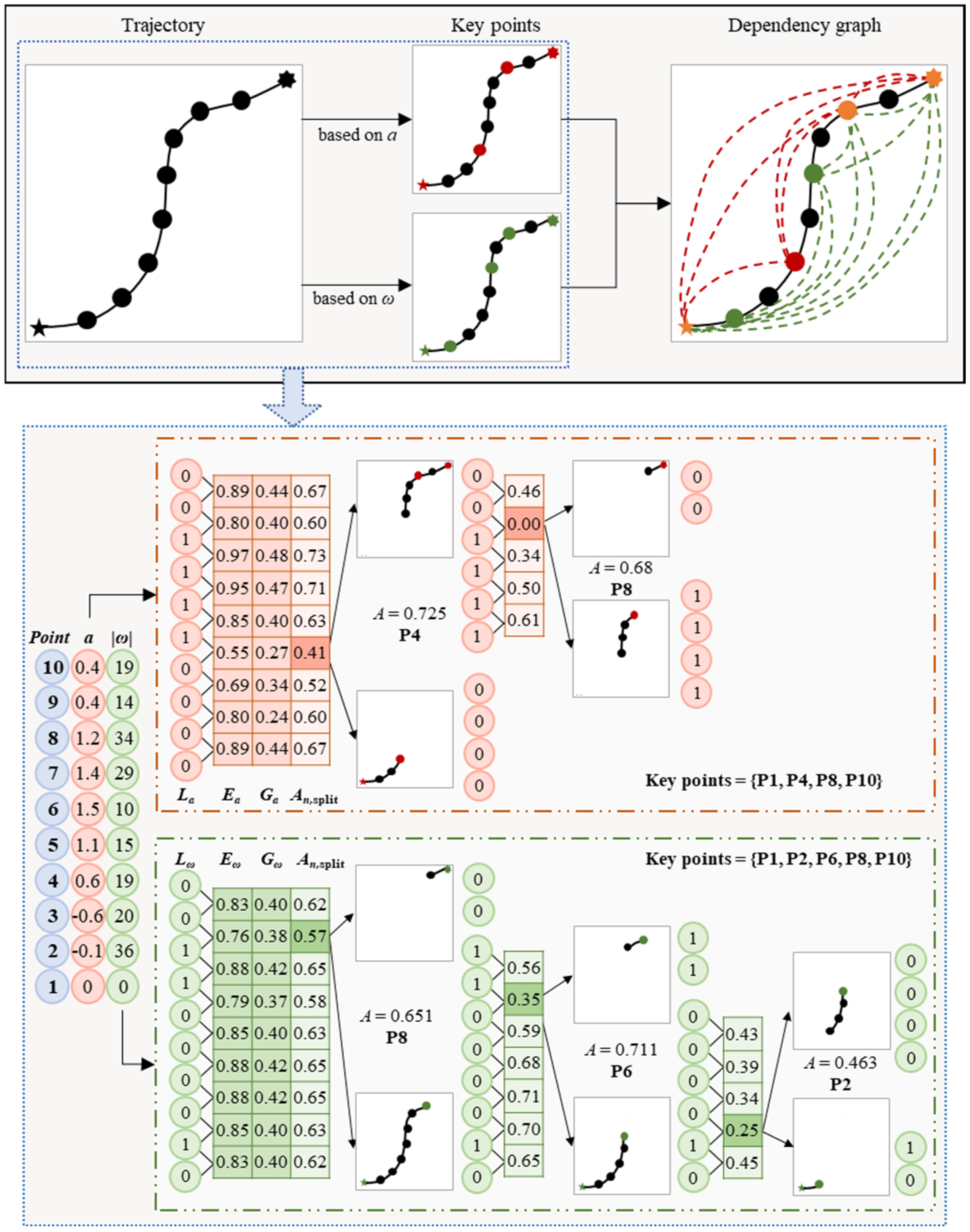
3.2.3. Selection Key Nodes

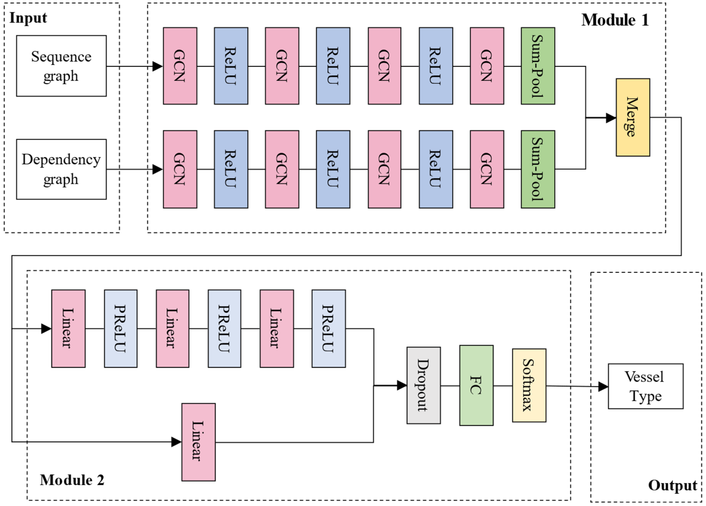
When constructing dependency graphs to define the dependencies between trajectory points, the selection of key nodes is crucial. For any given vessel trajectory, this typically includes a starting point, an ending point, and some intermediate points. In addition to the start/end point, we define key nodes as those places where there are significant changes in direction or speed, as these points highlight the characteristics of the trajectory path.

In land-based traffic, the direction change of the trajectories usually occurs at intersections, so the intersections of the road network are often regarded as key nodes. However, maritime traffic is different from land traffic, which has no fixed road network structure. Therefore, based on the method proposed in a previous study [32], we determine the key nodes of the vessel in the two dimensions of speed and direction, according to the $a$ and $\omega$ of the trajectory point. The change of these two features can reflect the behavior state of different trajectories, which provides a basis for distinguishing the different types of trajectories.

To accurately identify the key feature points, we must understand the dynamic changes in the vessel’s $a$ and $\omega$. The specific calculation method is illustrated in Figure 4. Information entropy (IE) and the Gini index (GI), as indicators to quantify the amount of information and uncertainty of data, can evaluate the consistency of data distribution.

If X is a discrete random variable with finite value, then the probability distribution is $F\left(X=x_i\right)=f_i$, the IE is $E(X)=-{\displaystyle \sum _{i=1}^n}{f}_i\log f_i$, the GI is $G(X)=1-{\displaystyle \sum _{i=1}^n}{f}_i^2$, and $i=1,2,\cdots ,n$, A larger value of IE indicates the higher uncertainty of the data. The closer the GI value is to 1, the more scattered the data points are.

The positive or negative of $a$ directly represents acceleration or deceleration, while the positive or negative of $\omega$ here represents only the direction of rotation and does not involve an increase or decrease in speed. Therefore, this paper combines EI and the GI to quantify the numerical distribution of $a$ and $\left|\omega \right|$. Then, this is used to assess changes in the speed and heading of vessel trajectories, thereby effectively extracting the key feature points. First, the K-means clustering method is used to cluster the $a$ of the trajectory, obtaining the acceleration range of the trajectory, and assigning an acceleration label $L_{i,a}$ to each trajectory point, based on this method. The IE of the vessel trajectory’s $a$ is calculated as $E_{n,a}(\begin{array}{c}T)\end{array}=-{\displaystyle \sum _{i=1}^n}(s_i{\log }_2{s}_i)$, $s_i={\displaystyle \raisebox{1ex}{$N(L_{i,a})$}\!\left/ \!\raisebox{-1ex}{$\left|L_a\right|$}\right.}$, where $s_i$ represents the frequency of occurrence of various speed labels in $L_a$, $\left|L_a\right|$ represents the overall count of acceleration labels, and $N(L_{i,a})$ denotes the aggregate frequency at which a specific identical label manifests within $L_a$. Similarly, the GI for the trajectory’s acceleration is calculated as $G_{n,a}(T)$.

We know that for any given trajectory, when each trajectory point has a distinct value for a certain feature, the calculated information entropy is at its maximum. By combining IE and GI, we can obtain the information content $A_n=\left(E_{n,a}(\begin{array}{c}T)\end{array}+G_{n,a}(T)\right)÷2$ of the entire trajectory. There is at least one position in the trajectory where the difference between two sub-trajectories is maximized, which serves as our basis for identifying the key nodes. Therefore, the trajectory $T_{1,n-1}$ is segmented at the $i\left(1\le i\le n-1\right)$ trajectory point; then, the information content $A_{n,\mathrm{split}}(\begin{array}{c}{T}_{1,n-1})\end{array}$ of the sub-trajectory is calculated according to the equation. The specific calculation formula is as follows:

$$A_{n,\mathrm{split}}(\begin{array}{c}{T}_{1,n-1})\end{array}={\displaystyle \frac{N_1}{N}}\left(A_{1,i}^{\prime }\right)+{\displaystyle \frac{N_2}{N}}\left(A_{i+1,n-1}^{\prime }\right)$$

(3)

$$A^{\prime }=\phi E_{n,a}(\begin{array}{c}T)\end{array}+(1-\phi )G_{n,a}(T)$$

(4)

where $A_{n,\mathrm{split}}(\begin{array}{c}{T}_{1,n-1})\end{array}$ represents the information content for each trajectory point, where $N_1$, $N_2$, and $N$ represent the number of trajectory points in $T_{1,i}$, $T_{i+1,n-1}$, and the entire trajectory $T_{1,n-1}$, respectively. $A^{\prime }$ is the information content of the sub-trajectory, and $\phi$ is a weight parameter with a value of 0.5.

When $A_n>\mathrm{threshold}$, this indicates that the trajectory has a high information content and the feature distribution is diverse. We then select the trajectory point with the minimum information content $A_{n,\mathrm{split}}({\begin{array}{c}{T}_{1,n-1})\end{array}}_{\min }$ as the key node. Based on this point, we segment the trajectory and continue to calculate the information content of the sub-trajectory segments using the aforementioned steps. We repeat this process until $A_n<\text{threshold}$, which indicates that all the key nodes for that trajectory segment have been extracted. We chose a threshold value of 0.3, based on previous experience [33].

Following the aforementioned steps, we can extract the key nodes of vessel trajectories. We then utilize the sequence and dependency relationships within the trajectory data to construct the two types of graphs, respectively. As depicted in Figure 4, there is a clear dependency between the key feature points, determined based on acceleration and angular velocity and the start/end point. These two types of dependency relationships together form the dependency graph, where the acceleration and angular velocity dependencies coexist in the same trajectory, which provides us with rich information about the vessel’s behavior.

3.3. Model Building

For this study, we constructed a vessel-type recognition model based on trajectory fusion representation, with the core framework as shown in Figure 5. Firstly, the constructed trajectory sequence graph data and dependence graph data were used as the input of the model. Secondly, we adopted the GCN (graph convolutional network) as the foundational framework for learning topological graph features. Through this training process, the model can comprehensively capture the node interaction and vessel behavior information on the graph. Subsequently, the multi-graph fusion strategy was used to effectively integrate the information from both the trajectory sequence graph and the dependency graph, generating a high-level feature for each trajectory. This feature not only includes the spatiotemporal behavior information of the vessel but also incorporates the dependency relation between trajectory points, thereby achieving a comprehensive and effective representation of vessel behavior. Finally, the vessel type recognition was realized, based on MLP.

3.3.1. Representative Fusion from Multiple Graphs

The GCN model is a multiple-layer neural network that is suitable for graph-structured data. Unlike the traditional CNN, the GCN can handle irregular data structures. It takes as input all the nodes, features, and adjacency relationships of the graph structure. By using edge information to aggregate node information, it generates new node representations. We can then use information from the nearby nodes to make inferences.

More specifically, the input of the model consists of two matrices: a feature matrix $X=N\times D$, where $N$ is the number of nodes and $D$ is the feature dimensions. The other is the $N\times N$-dimensional adjacency matrix $A$. $A$ is the neighbor relationships between nodes. The feature dimension $D=12$ can be identified according to the feature extraction. Since the number of key nodes in each trajectory segment extracted when building the dependency graph may vary, to facilitate unified calculation and processing, we set $N$ to be the count of points in the longest trajectory. Therefore, each vessel trajectory includes a starting point, an ending point, and some extracted feature points. For trajectories with fewer nodes than $N$, we use zero-padding for both the feature matrix and the adjacency matrix to ensure matrix dimensional consistency without introducing too much redundancy.

We use the GCN architecture to perform feature extraction of the constructed two types of graphs. As shown in Figure 5, the encoder section consists of four convolutional layers. The GCN layer is defined as $H^{(l+1)}=\sigma \left(\tilde{A}{H}^{(l)}{W}^{(l)}\right)$, which is used to learn the node representations for two sets of views separately.

Here, $\tilde{A}={\widehat{D}}^{-\frac{1}{2}}\widehat{A}{\widehat{D}}^{-\frac{1}{2}}$ represents the symmetrically normalized adjacency matrix, $\widehat{A}=A+I$, $I$ is the identity matrix, and $\widehat{D}$ is the degree matrix of $\widehat{A}$; $H^0=X$, $X$ is the node feature matrix, $W$ is the parameter matrix for each layer, and $\sigma \left(.\right)$ is a nonlinear activation function. We employ the ReLU (rectified linear unit) activation function to add nonlinear functions in the hidden layers, followed by a sum-pool (Sum Pooling) operation to aggregate node information. After that, we use a multi-graph fusion strategy to merge the node information obtained from the two graphs into a unified graph representation. The trajectory graph feature extraction model can be represented as:

$$h_g=\sigma \left({\Vert }_{g=1}^G\left[{\displaystyle {\sum }_{n=1}^N{h}_n^{\left(g\right)}}\right]W\right)$$

(5)

where $h_g$ represents the representation of the trajectory graph, $h_n^{\left(g\right)}$ denotes the feature representation of the n-th trajectory node within the g-th graph, $N$ is the total number of nodes, and $G$ is the total number of graphs, which, in this case, is the number of sequence and dependency graphs, $\Vert$ denotes feature concatenation, and $W$ represents the network parameters.

3.3.2. Classifier Construction

Subsequently, we input these graph feature vectors $h_g$ into a designed MLP. This MLP includes parallel hidden layer pathways. The former has three hidden layers, each using a nonlinear PreLU (parametric rectified linear unit) activation function to boost the model’s nonlinear capabilities. Running in parallel with this is a path with only one linear layer. This design aims to combine the advantages of capturing nonlinear expressions and linear relationships, improving the model’s flexibility and accuracy when dealing with complex data. Subsequently, the model introduces a dropout mechanism to reduce overfitting and enhance generalization ability. During the inference stage, a fully connected (FC) layer maps the extracted features to the trajectory pattern type space, and then the softmax activation function outputs the probability distribution of each trajectory belonging to the different vessel categories. We used a semi-supervised method for model training and chose cross-entropy loss, which is widely used in classification tasks, as the loss function.

3.4. Evaluation Indicators

To comprehensively evaluate the effect of vessel trajectory type recognition, we used some key indicators that are commonly used in classification tasks for comprehensive evaluation, such as accuracy, precision, recall, F1 score, and the confusion matrix. Accuracy represents the proportion of correctly classified vessels, precision indicates the proportion of true positives among all positive classified instances, recall shows the proportion of true positives among all actual positive instances, the F1 score is the harmonic mean of precision and recall, and the confusion matrix provides an intuitive view of the performance of the analysis model in each category. To facilitate statistical comparison, we use the average value of each indicator as the comparison indicator, and the calculation equation is as follows:

$$\left\{\begin{array}{l}A={\displaystyle \frac{1}{N}}{\displaystyle \sum _i^N\frac{T{P}_i+T{N}_i}{T{P}_i+T{N}_i+F{P}_i+F{N}_i}}\\ P={\displaystyle \frac{1}{N}}{\displaystyle \sum _i^N\frac{T{P}_i}{T{P}_i+F{P}_i}}\\ R={\displaystyle \frac{1}{N}}{\displaystyle \sum _i^N\frac{T{P}_i}{T{P}_i+F{N}_i}}\\ F={\displaystyle \frac{1}{N}}{\displaystyle \sum _i^N\frac{2P_i{R}_i}{P_i+R_i}}\end{array}\right.$$

(6)

where $A,P,R,F$ represents the average accuracy, the average precision, the average recall, and the average F1 score. $T{P}_i$ is the number of true positives for the i-th class of vessel types; $F{P}_i$ is the number of false positives; $T{N}_i$ is the number of true negatives; $F{N}_i$ is the number of false negatives. By using these evaluation indicators, we can comprehensively evaluate the effect of the vessel trajectory type recognition to verify the effectiveness of the model.

4. Experiments and Evaluation

4.1. Research Area and Datasets

In this study, two specific ocean regions were selected as the main study areas. Among them, study area 1 is located in the western ocean area of North America, and the latitude and longitude range is defined between 68.84° W to 78.84° W and 34.56° N to 42.58° N. Study area 2 is located in the eastern ocean area of North America, and its latitude and longitude span from 121.80° W to 128.21° W and 40.10° N to 50.34° N. The AIS data of July 2021, provided by the National Oceanic and Atmospheric Administration (NOAA), were used for the experimental data. The location and trajectory distribution of the specific study area are shown in Figure 6.

The relationship between vessel type code and vessel type is shown in

Table 1. Vessel types and vessel type codes (https://coast.noaa.gov/data/marinecadastre/ais/VesselTypeCodes2018.pdf) (accessed on 1 December 2024).

Vessel Type	Vessel Type Code
Cargo	70–79, 1003, 1004
Fishing	30, 1001, 1002
Passenger	60–69, 1012–1015
Tug/Tow	21, 22, 31, 32, 52, 1023
Pleasure Craft	36, 37, 1019

. After conducting statistical analysis on the downloaded AIS data, we found that the five main vessel types—cargo, fishing, passenger, tug/tow, and pleasure craft—account for 88.52% of the total data. Therefore, we primarily extracted and analyzed the trajectory data of these five vessel types. The statistical data thus obtained are shown in

Table 2. Statistical information of the various types of vessels.

Vessel Type	Dataset-1		Dataset-2
	Number of Trajectory Points	Number of Trajectories	Number of Trajectory Points	Number of Trajectories
Cargo	1,295,153	1804	1,211,478	1503
Fishing	328,378	592	658,165	446
Passenger	1,657,198	3579	994,217	2223
Tug/Tow	1,750,639	2572	1,680,430	1650
Pleasure Craft	393,193	1212	630,024	806

.

4.2. Parameter Settings and Experimental Results

4.2.1. Parameter Settings

During the data preprocessing stage, to ensure that the number of points in each trajectory segment was uniform, we divided the trajectories into a fixed length. This not only ensured the consistency of trajectory information but also facilitated the comparison of the recognition effect of the model for different trajectory types. We divided the two sets of data to construct the model dataset by using 20 and 30 points as the division criteria of a trajectory segment, respectively. The dataset was randomly partitioned into a training set, a test set, and a validation set, with proportions of 60%, 20%, and 20%, respectively. We used PyTorch to implement our designed model and to conduct experiments on the following hardware platforms (CPU: Intel Xeon Gold 6230 and GPU: NVIDIA GeForce RTX 3090). Through many experiments, we finally determined the parameter settings of the model, as follows. We trained the model using the Adam optimizer. The empirical initial learning rate and L2 normalization parameter were set to 0.001, the batch size was set to 256, the number of epochs was set to 300, hidden units were set to 64, and the dropout rate parameter was set to 0.4.

4.2.2. Result Analysis

We used the dataset of 30-point trajectory segments as our benchmark dataset for model training. As the number of epochs increased, the loss function value eventually decreased and tended to stabilize. The validation losses for the two datasets were 0.4004 and 0.4915, and the test losses on the test sets were 0.4117 and 0.4755, with test accuracies reaching 85.39% and 83.22%, respectively. This proves the effectiveness of our model.

To further verify the reliability of the proposed method, we set the number of points of each vessel trajectory to 20 to conduct comparative experiments. Generally, a reduction in the number of vessel trajectory points led to a diminished amount of feature information in the trajectory, which made the recognition task more difficult. Under the same experimental parameter settings, we found that when using the dataset with 20 trajectory points for testing, the accuracy still reached 84.07% and 82.13%. The respective metric values are shown in

Table 3. Evaluation indicator comparison results.

Dataset	Points	A	P	R	F
Dataset-1	20	84.07%	81.09%	75.82%	77.99%
	30	85.39%	82.46%	78.01%	79.83%
Dataset-2	20	82.13%	82.40%	80.90%	81.53%
	30	83.22%	83.47%	82.01%	82.65%

.

As shown in Figure 7, although the indicator values calculated for the dataset with 20 trajectory points were lower than those for the dataset with 30 trajectory points, all accuracy metrics still maintained a high level above 80%. This result not only indicates that the model in our approach can capture the trajectory distribution features of different vessel types from AIS data but also further proves that the model has good robustness.

Additionally, we obtained the results of the vessel trajectory type identification and plotted the normalized probability matrix, as shown in Figure 8 and Figure 9. By comparing the results of the two datasets, we can observe that the model achieves high accuracy in identifying the types of cargo, passenger, and tug/tow vessels, all exceeding 80%. Typically, an uneven distribution of sample counts across different classes can impair the classification accuracy of a model. This imbalance may cause certain ambiguous data features to be more frequently misclassified as belonging to a class with a higher number of samples.

The identification accuracy rates for fishing and pleasure craft vessels are slightly lower. As the number of trajectory points decreases, the accuracy regarding pleasure craft declines more noticeably. The accuracy rates for the other types of vessels show relatively minor fluctuations. This is primarily due to the relatively smaller number of pleasure craft vessel trajectory samples.

In order to analyze this phenomenon, we took the number of pleasure craft vessels as the baseline and set them to 20%, 50%, and 100% respectively, and resampled the number of other vessel types, so that the amount of data of each type was consistent. However, under this balanced data setting, the classification accuracy was 49.83%, 71.67%, and 76.20% respectively, which instead showed a decrease. Through this analysis, we found that when the number of vessels is balanced, the true distribution and structure of the data are ignored, which leads to the model overly relying on the resampled data distribution and ignoring the inherent class imbalance in the original data. This processing method makes the model unable to effectively capture the actual differences between different vessel types in the training process and then leads to the imperfect feature extraction of some vessel types, which affects the recognition performance of the model.

Additionally, in real life, pleasure craft vessels typically have fewer activity restrictions compared to other types of vessels and often do not follow fixed routes or predetermined itineraries. As a result, their movements may be more arbitrary, and their trajectories are often more irregular, which can lead to overlaps with the trajectories of other types of vessels. When the number of trajectory points decreases, the sequence and dependency relationships also correspondingly diminish, which further increases the risk of misclassifying pleasure craft into similar types.

In summary, our model is capable of demonstrating good performance across different levels of segmentation granularity and can effectively distinguish between various vessel types. However, for certain specific types of vessels, such as pleasure craft, the recognition accuracy of the model may be impacted due to the complexity of their trajectory characteristics and the limited sample size.

4.3. Comparison with Other Methods

4.3.1. Comparative Methods

We chose a variety of methods for the comparative experiments, which were used to further comprehensively evaluate the effectiveness and feasibility of the model. There are 10 methods that were selected, including classical machine learning methods and deep learning methods in other works of literature.

• DT. DT models data classification through a tree structure that simulates conditional branching [34]. Each intermediate node represents a judgment regarding a certain attribute, each branch represents the output of the result, and, ultimately, each leaf node represents a categorization result. To facilitate computation, we extracted the maximum and minimum values, as well as the average values, of all point features for each trajectory segment. These values were used as the primary features, and the data were then flattened into one-dimensional features to serve as the input features for the model.
• RF. RF is an ensemble learning algorithm that operates by constructing multiple decision trees and aggregating their classification results [16,35].
• KNN. KNN is a simple classification algorithm based on proximity, which identifies the category of a point by looking at the categories of its nearest K neighboring samples [36].
• SVM. SVM is a supervised learning algorithm that conducts classification by finding the optimal hyperplane in the feature space that maximizes the margin between different classes [15,37].
• MLP. MLP, as the simplest form of a feedforward neural network model, includes multiple hidden layers in addition to the input and output layers.
• The 1D convolutional neural network (1D-CNN). The 1D-CNN can automatically extract important features from the data for type recognition [28]. We used only the extracted $N\times 12$ feature matrix as the model input features.
• LSTM. LSTM is a type of RNN model that is capable of learning and remembering long-term dependencies, and it is widely used for sequential data [27]. In classification tasks, the network parameters can be optimized using the cross-entropy loss function.
• GCN. The GCN model learns node representations by aggregating the neighbors of nodes in a graph while taking into account the node’s features and the structural information of the graph. We only utilized the basic GCN model for comparison, using sequence graph data as the input. To maintain consistency when comparing models, all other parameter configurations were kept uniform.
• The 1DCNN-LSTM (C-L). The C-L is a hybrid deep learning model that can capture both local features and long-term dependencies in data. This makes the C-L model very effective in handling complex sequence classification problems [29].
• LSTM-GCN (L-G). We adopted an LSTM module instead of a single GCN module to extract the sequence features, which were combined with the dependent features extracted by another GCN module.

Among them, the model inputs of RF, KNN, SVM, and MLP are the same as DT, and the model inputs of LSTM and C-L are the same as the 1D-CNN inputs.

4.3.2. Comparative Analysis of Recognition Results

Based on two datasets (trajectories containing 30 points and 20 points), we carried out comparative experiments on the aforementioned models. The comparison was made using the same datasets for all methods, ensuring consistency in evaluation. The key evaluation metric results are summarized in

Table 4. Comparison of the evaluation indicators between different methods for Dataset-1.

Methods	Point = 30				Point = 20
	A	P	R	F	A	P	R	F
DT	70.91%	71.46%	54.21%	55.80%	70.79%	70.21%	54.00%	55.43%
RF	72.02%	71.62%	55.64%	57.63%	72.75%	71.43%	57.69%	59.82%
KNN	71.42%	64.01%	61.23%	62.44%	71.84%	65.01%	62.45%	63.49%
SVM	58.93%	58.48%	41.21%	40.05%	59.66%	55.23%	41.49%	40.46%
MLP	71.20%	65.24%	59.01%	60.42%	70.81%	68.00%	56.51%	59.23%
1D-CNN	76.36%	73.77%	63.68%	66.27%	72.98%	70.41%	57.87%	60.58%
LSTM	78.77%	75.25%	65.97%	68.72%	79.82%	75.54%	68.66%	70.96%
GCN	79.06%	76.61%	66.68%	69.37%	80.25%	76.06%	70.20%	71.97%
C-L	79.51%	73.47%	71.45%	72.22%	81.15%	83.83%	69.18%	73.40%
L-G	80.51%	75.26%	72.93%	73.46%	80.92%	79.75%	70.84%	73.96%
OUR	85.39%	82.46%	78.01%	79.83%	84.07%	81.09%	75.82%	77.99%

and

Table 5. Comparison of evaluation indicators between the different methods for Dataset-2.

Methods	Point = 30				Point = 20
	A	P	R	F	A	P	R	F
DT	72.91%	75.63%	71.81%	72.41%	72.83%	74.00%	72.21%	72.69%
RF	67.25%	68.85%	66.87%	66.22%	65.98%	67.00%	66.68%	65.00%
KNN	67.38%	66.47%	65.83%	66.03%	67.93%	67.29%	66.66%	66.89%
SVM	49.00%	36.44%	35.82%	31.81%	50.18%	54.26%	37.89%	36.11%
MLP	68.29%	66.85%	68.28%	67.67%	68.89%	69.00%	66.23%	67.27%
1D-CNN	70.75%	71.46%	67.98%	69.30%	73.61%	73.75%	71.88%	72.68%
LSTM	76.48%	76.36%	74.88%	75.51%	75.45%	76.21%	73.79%	74.80%
GCN	75.90%	76.09%	74.13%	74.94%	76.47%	77.69%	74.25%	75.68%
C-L	68.71%	66.26%	60.80%	59.70%	80.39%	83.03%	77.59%	79.75%
L-G	81.43%	81.95%	80.02%	80.75%	81.55%	82.14%	80.18%	80.93%
OUR	83.22%	83.47%	82.01%	82.65%	82.13%	82.40%	80.90%	81.53%

. Through comparison, it can be seen that regardless of whether the trajectory points are 30 or 20, our model outperforms the other models in terms of recognition results.

To show the comparison effect of each model index value more intuitively, we drew the index comparison chart of the model recognition results in the case of 30 trajectory points. As depicted in Figure 10, it can be seen that our model outperforms others across all metrics, with particularly notable advantages in terms of recognition accuracy. Furthermore, our model also demonstrates superior metric values in the other three evaluation indicators. This further confirms the superiority of our proposed model in recognition tasks.

For ease of overall comparison, we plotted the normalized probability matrices of the recognition results of the other methods, as shown in Figure 11 and Figure 12. The value of each cell in the matrix represents the ratio of the number of correctly identified positive instances to the total number of actually marked positive instances. From the matrix diagram, it can be observed that the traditional machine learning models of DT, RF, KNN, SVM, and MLP yield similar performance matrices, all of which are inferior to those obtained by deep learning models. Among them, the SVM model exhibits the poorest identification effectiveness, with fishing and pleasure craft vessels being almost unrecognizable. In contrast, deep learning models demonstrate better identification results; the matrices obtained by 1DCNN, LSTM, GCN, C-L, L-G, and our model are more similar to each other.

When experimenting with hybrid models such as C-L and L-G, we found that setting the hidden layers of the model to be the same would lead to overfitting. Therefore, to facilitate comparison, we set the size of the hidden layers to 48 or smaller. However, as shown in Figure 12, the C-L model hardly recognized any fishing-type vessels, and the overall matrix generated by the model was not as effective as the recognition results from single models. The L-G model architecture simply replaced the GCN-extracted sequence graph module with an LSTM model to extract the temporal relationships. Although the recognition accuracy for some types of vessels improved, overall, it still did not perform as well as our model.

Integrating the analysis from Figure 11 and Figure 12, we can observe that in various comparative experiments, the recognition accuracy for the cargo, passenger, and tug/tow types of vessels was generally high. Our method demonstrates even better recognition accuracy rates for these types. For fishing and pleasure craft vessels, although the recognition accuracy of all models is relatively lower, our model still shows a higher degree of accuracy, proving the effectiveness of our approach in fully leveraging the features of vessel trajectories.

In summary, our method is not only able to provide better vessel type recognition results as a whole but also shows a stronger ability to deal with complex or difficult-to-identify vessel types. This fully verifies the superiority and reliability of our method in effectively distinguishing the current vessel types.

4.4. Ablation Study

To verify the performance contribution of each module in the vessel type recognition model, we designed ablation experiments with consistent experimental parameter settings. Specifically, we conducted four comparative experiments: (1) without the sequence graph construction block (WO-S); (2) without the dependency graph construction block (WO-D); (3) without the MLP block; (4) full model (OUR). Through the evaluation indicators in

Table 6. Comparison of evaluation indicators of the ablation study for Dataset-1.

Methods	Point = 30				Point = 20
	A	P	R	F	A	P	R	F
WO-S	77.38%	71.68%	67.80%	68.95%	78.34%	73.51%	69.07%	70.47%
WO-D	82.52%	79.57%	72.16%	74.46%	82.65%	78.44%	74.75%	76.01%
WO-M	74.78%	71.34%	61.91%	64.03%	74.16%	71.80%	61.31%	63.48%
OUR	85.39%	82.46%	78.01%	79.83%	84.07%	81.09%	75.82%	77.99%

and

Table 7. Comparison of evaluation indicators of the ablation study for Dataset-2.

Methods	Point = 30				Point = 20
	A	P	R	F	A	P	R	F
WO-S	68.11%	71.43%	63.37%	65.85%	72.30%	74.91%	69.71%	71.55%
WO-D	79.26%	78.93%	78.44%	78.63%	77.83%	78.56%	75.80%	76.97%
WO-M	70.89%	71.15%	69.11%	69.90%	71.38%	72.08%	69.43%	70.36%
OUR	83.22%	83.47%	82.01%	82.65%	82.13%	82.40%	80.90%	81.53%

, we can observe that across multiple test datasets, when each of these three key modules was removed, there was a noticeable decline in recognition accuracy and other related indicators.

To facilitate a clearer assessment of the performance of each module within the model, we plotted a comparison chart of the model evaluation indicators under the condition of 30 trajectory points, as shown in Figure 13. Combining Table 6 and Table 7 with Figure 13, we can observe that the WO-D model’s recognition effect is second only to the complete model, while the other two models perform poorly in terms of recognition. Looking at the evaluation indicators from Dataset 1, the MLP block has the greatest impact on the recognition results, with an accuracy improvement of 10.61%. Following that is the sequence graph construction block, which can enhance the accuracy by 8.01%. On Dataset 2, the sequence graph construction block shows the greatest impact, with an accuracy improvement of 15.11%. Next is the MLP block, which improves the accuracy by 12.33%. These fully demonstrate that each module can improve the performance of the model on different datasets.

Similarly, we plotted the normalized probability matrices for the comparison models’ recognition results on the dataset with 30 trajectory points, as shown in Figure 14 and Figure 15. It is evident from the diagrams that our complete model has the highest recognition accuracy for all vessel types. In both datasets, all methods have relatively higher recognition accuracy rates for the cargo, passenger, and tug/tow types of vessels. Our method achieves an even higher level of recognition accuracy for these three types, demonstrating a more outstanding overall performance. For fishing and pleasure craft vessels, our model shows an increase in accuracy on both datasets, with a more pronounced improvement in Dataset 1.

In summary, our proposed method effectively integrates the sequence graph construction module, the dependency graph construction module, and the multi-layer perceptron module. This integration can make more comprehensive use of the spatiotemporal and semantic features of vessel trajectories, leading to a higher level of vessel type identification effectiveness. The multi-layer perceptron module, serving as a type decoder, plays an essential role in vessel type recognition. The sequence graph construction module effectively extracts the spatiotemporal features of vessel trajectories, while the dependency graph construction module enhances the precision of vessel type recognition by filtering and extracting the spatiotemporal information of key feature points. These findings not only confirm the effectiveness of each module but also provide a strong basis for future model optimization.

5. Conclusions

In this study, we proposed a multi-graph representation method that integrated the trajectory sequence and dependency relationships for the recognition of vessel types. This method combines trajectory sequences and dependency relationships. The experiments have fully demonstrated that our method can not only learn complex embedded representations of trajectory data but also perform better in vessel trajectory type recognition tasks, with accuracy rates exceeding those of other comparative methods.

The advantages of this method are reflected in the following three aspects: (1) it can mine the relationships between trajectory feature points from trajectory data, providing abundant vessel behavior information for trajectory type recognition. The sequence relation maintains the original order of the trajectory points, which helps capture positional change information. Meanwhile, the dependency relation expresses the correlation between trajectory points, aiding in obtaining contextual semantic change information about the trajectory. (2) We have introduced a multi-graph convolutional network model that can extract high-order features with vessel trajectory behavior from spatiotemporal and contextual information. By representing both relationships graphically and by aggregating trajectories into representation vectors, we can more effectively capture the discriminative elements of various types of trajectories. (3) The developed method demonstrates versatility and is applicable to trajectory data of different scales. When dealing with irregularly sampled AIS data, we utilized graph convolutional networks, avoiding cumbersome interpolation and resampling processes, thereby preserving the original attribute features of the data. The experimental results show that even with different numbers of trajectory points (such as 30 points or 20 points), this method can still achieve satisfactory identification results.

In future work, our method has the potential to be extended to more detailed classifications. (1) For instance, building upon the recognition of vessel types, we can further incorporate various environmental and conditional factors to conduct an in-depth analysis and recognition of vessel behavior patterns. (2) The class imbalance of vessel types is a common problem in AIS data. Some vessel types occupy a large proportion of the data, while others are scarce, and this unbalanced distribution may cause the classification model to be biased during training. Specifically, the model may tend to make more accurate predictions for those vessel types that are overrepresented and ignore those that occur less frequently, thus affecting the overall classification performance and reducing the fairness and accuracy of the model. In future work, we can compensate for the bias of class imbalance by assigning different importance values to different classes during training by class weighting. Another possible strategy is oversampling, which increases the number of samples in the minority class to balance the distribution of the training data. (3) In addition, in the actual maritime environment, the behavior between vessels is not only affected by individual features but also by the spatial positions between each other, their navigation trajectory, and the surrounding environment. Therefore, an in-depth study of the spatiotemporal interactions between neighboring ships can help us better understand the mutual influence of ship behavior and, thus, improve the accuracy of behavior prediction and decision support ability. When it comes to large-scale AIS datasets, we will explore techniques such as distributed processing, data sampling, and model compression to cope with large datasets. (4) Additionally, we can explore the fusion of multimodal trajectory data. By integrating information from different sensors and data sources (such as satellite imagery, radar data, video data, and AIS data), we can obtain a more comprehensive representation of vessel behavior. The fusion of multimodal data will help enhance the model’s robustness and accuracy, enabling better performance in complex maritime environments. (5) Lastly, we plan to assess the model’s potential in different downstream applications, such as anomaly detection. By extensively applying and validating its use in real-world scenarios, we aim to further explore and showcase the significant value of this method in the realms of maritime management and intelligent transportation systems. This will offer essential technical support and decision-making foundations for future maritime management and intelligent transportation systems.

References

1. Kim, H.; Lee, E.; Lee, E.; Hyun, J.; Gong, I.; Kim, K.; Lee, Y. A Study on Grid-Cell-Type Maritime Traffic Distribution Analysis Based on AIS Data for Establishing a Coastal Maritime Transportation Network. J. Mar. Sci. Eng. 2023, 11, 354. [Google Scholar] [CrossRef]
2. Ferreira, M.D.; Campbell JN, A.; Matwin, S. A novel machine learning approach to analyzing geospatial vessel patterns using AIS data. GISci. Remote Sens. 2022, 59, 1473–1490. [Google Scholar] [CrossRef]
3. Zou, Y.; Zhang, Y.; Wang, S.; Jiang, Z.; Wang, X. Ship regulatory method for maritime mixed traffic scenarios based on key risk ship identification. Ocean Eng. 2024, 298, 117105. [Google Scholar] [CrossRef]
4. Rapalis, P.; Šilas, G.; Žaglinskis, J. Ship Air Pollution Estimation by AIS Data: Case Port of Klaipeda. J. Mar. Sci. Eng. 2022, 10, 1950. [Google Scholar] [CrossRef]
5. Meyers, S.D.; Yilmaz, Y.; Luther, M.E. Some methods for addressing errors in static AIS data records. Ocean Eng. 2022, 264, 112367. [Google Scholar] [CrossRef]
6. Gupta, P.; Rasheed, A.; Steen, S. Correlation-based outlier detection for ships’ in-service datasets. J. Big Data 2024, 11, 85. [Google Scholar] [CrossRef]
7. Gaglione, D.; Soldi, G.; Meyer, F.; Hlawatsch, F.; Braca, P.; Farina, A.; Win, M.Z. Bayesian information fusion and multitarget tracking for maritime situational awareness. IET Radar Sonar Navig. 2020, 14, 1845–1857. [Google Scholar] [CrossRef]
8. Petković, M.; Vujović, I.; Kaštelan, N.; Šoda, J. Every Vessel Counts: Neural Network Based Maritime Traffic Counting System. Sensors 2022, 23, 6777. [Google Scholar] [CrossRef]
9. Wolsing, K.; Roepert, L.; Bauer, J.; Wehrle, K. Anomaly Detection in Maritime AIS Tracks: A Review of Recent Approaches. J. Mar. Sci. Eng. 2021, 10, 112. [Google Scholar] [CrossRef]
10. Wang, Y.; Liu, J.; Liu, R.W.; Liu, Y.; Yuan, Z. Data-driven methods for detection of abnormal ship behavior: Progress and trends. Ocean Eng. 2023, 271, 113673. [Google Scholar] [CrossRef]
11. Mazzarella, F.; Vespe, M.; Alessandrini, A.; Tarchi, D.; Aulicino, G.; Vollero, A. A novel anomaly detection approach to identify intentional AIS on-off switching. Expert Syst. Appl. 2017, 78, 110–123. [Google Scholar] [CrossRef]
12. Kurekin, A.A.; Loveday, B.R.; Clements, O.; Quartly, G.D.; Miller, P.I.; Wiafe, G.; Adu Agyekum, K. Operational Monitoring of Illegal Fishing in Ghana through Exploitation of Satellite Earth Observation and AIS Data. Remote Sens. 2018, 11, 293. [Google Scholar] [CrossRef]
13. Ribeiro, C.V.; Paes, A.; Oliveira, D.D. AIS-based maritime anomaly traffic detection: A review. Expert Syst. Appl. 2023, 231, 120561. [Google Scholar] [CrossRef]
14. Weerakody, P.B.; Wong, K.W.; Wang, G.; Ela, W. A review of irregular time series data handling with gated recurrent neural networks. Neurocomputing 2021, 441, 161–178. [Google Scholar] [CrossRef]
15. Yan, Z.; Song, X.; Zhong, H.; Yang, L.; Wang, Y. Ship Classification and Anomaly Detection Based on Spaceborne AIS Data Considering Behavior Characteristics. Sensors 2022, 22, 7713. [Google Scholar] [CrossRef]
16. Huang, I.; Lee, M.; Nieh, C.; Huang, J. Ship Classification Based on AIS Data and Machine Learning Methods. Electronics 2024, 13, 98. [Google Scholar] [CrossRef]
17. Yang, T.; Wang, X.; Liu, Z. Ship Type Recognition Based on Ship Navigating Trajectory and Convolutional Neural Network. J. Mar. Sci. Eng. 2021, 10, 84. [Google Scholar] [CrossRef]
18. Seong, N.; Kim, J.; Lim, S. Graph-Based Anomaly Detection of Ship Movements Using CCTV Videos. J. Mar. Sci. Eng. 2023, 11, 1956. [Google Scholar] [CrossRef]
19. Li, T.; Xu, H.; Zeng, W. Ship Classification Method for Massive AIS Trajectories Based on GNN. J. Phys. Conf. Ser. 2021, 2025, 012024. [Google Scholar] [CrossRef]
20. Kong, Z.; Cui, Y.; Xiong, W.; Xiong, Z.; Xu, P. Ship Target Recognition Based on Context-Enhanced Trajectory. ISPRS Int. J. Geo-Inf. 2022, 11, 584. [Google Scholar] [CrossRef]
21. Ristic, B.; La Scala, B.; Morelande, M.; Gordon, N. Statistical analysis of motion patterns in AIS data: Anomaly detection and motion prediction. In Proceedings of the 11th International Conference on Information Fusion, Cologne, Germany, 30 June–3 July 2008; pp. 1–7. [Google Scholar]
22. Kraus, P.; Mohrdieck, C.; Schwenker, F. Ship classification based on trajectory data with machine-learning methods. In Proceedings of the 19th International Radar Symposium (IRS), Bonn, Germany, 20–22 June 2018; pp. 1–10. [Google Scholar]
23. Lang, H.; Wu, S.; Xu, Y. Ship classification in SAR images improved by AIS knowledge transfer. IEEE Geosci. Remote Sens. Lett. 2018, 15, 439–443. [Google Scholar] [CrossRef]
24. Ginouhac, R.; Barbaresco, F.; Scheider, J.; Pannier, J.M.; Savary, S. Coastal radar target recognition based on kinematic data (AIS) with machine learning. In Proceedings of the 2019 International Radar Conference (RADAR), Toulon, France, 23–27 September 2019; pp. 1–5. [Google Scholar] [CrossRef]
25. Wang, B.; Wand, Y.; Qin, K.; Xia, Q. Detecting Transportation Modes Based on LightGBM Classifier from GPS Trajectory Data. In Proceedings of the 2018 26th International Conference on Geoinformatics, Kunming, China, 28–30 June 2018; pp. 32–41. [Google Scholar]
26. Guo, T.; Xie, L. Research on Ship Trajectory Classification Based on a Deep Convolutional Neural Network. J. Mar. Sci. Eng. 2022, 10, 568. [Google Scholar] [CrossRef]
27. Llerena, J.P.; García, J.; Molina, J.M. LSTM vs. CNN in real ship trajectory classification. Log. J. IGPL 2024. [Google Scholar] [CrossRef]
28. Wang, Y.; Yang, L.; Song, X. A Multi-Feature Ensemble Learning Classification Method for Ship Classification with Space-Based AIS Data. Appl. Sci. 2020, 11, 10336. [Google Scholar] [CrossRef]
29. Syed, M.A.; Ahmed, I. A CNN-LSTM Architecture for Marine Vessel Track Association Using Automatic Identification System (AIS) Data. Sensors 2022, 23, 6400. [Google Scholar] [CrossRef]
30. Yuan, J.; Zhang, Q.; Zhang, J.; Li, Y.; Liu, Z.; Xue, M.; Zeng, Y. Fishing Vessel Type Recognition Based on Semantic Feature Vector. Int J. Data Warehous. Min. 2024, 20, 1–18. [Google Scholar] [CrossRef]
31. Ye, L.; Chen, X.; Liu, H.; Zhang, R.; Li, J.; Lu, C.; Zhao, Y. A Study of Multi-Step Sparse Vessel Trajectory Restoration Based on Feature Correlation. Appl. Sci. 2024, 14, 4057. [Google Scholar] [CrossRef]
32. Shin, G.; Yang, H. Vessel trajectory prediction in harbors: A deep learning approach with maritime-based data preprocessing and Berthing Side Integration. Ocean Eng. 2024, 316, 119908. [Google Scholar] [CrossRef]
33. Ye, L.; Chen, X.; Zhang, R.; Zhang, B.; Liu, H. An adaptive trajectory segmentation and simplification algorithm based on vessel behavioral features. Ocean Eng. 2024, 312, 119329. [Google Scholar] [CrossRef]
34. Quinlan, J.R. Induction of decision trees. Mach. Learn. 1986, 1, 81–106. [Google Scholar] [CrossRef]
35. Breiman, L. Random forests. Mach. Learn. 2001, 45, 5–32. [Google Scholar] [CrossRef]
36. Peterson, L.E. K-nearest neighbor. Scholarpedia 2009, 4, 1883. [Google Scholar] [CrossRef]
37. Cortes, C.; Vapnik, V. Support-Vector Networks. Mach. Learn. 1995, 20, 273–297. [Google Scholar] [CrossRef]
Figure 1. Flowchart of the experimental method.
Jmse 12 02315 g001
Figure 2. Flowchart of data preprocessing.
Jmse 12 02315 g002
Figure 3. Flowchart of graph construction for determining vessel trajectory.
Jmse 12 02315 g003
Figure 4. Flowchart of key node selection.
Jmse 12 02315 g004
Figure 5. Model architecture.
Jmse 12 02315 g005
Figure 6. Trajectory distribution in the experimental area: (A) Study area-1; (B) Study area-2.
Jmse 12 02315 g006
Figure 7. Comparison of the evaluation indicators.
Jmse 12 02315 g007
Figure 8. The normalized probability matrix of the vessel recognition results for Dataset-1: (A) the matrix map with points = 20; (B) the matrix map with points = 30.
Jmse 12 02315 g008
Figure 9. The normalized probability matrix of vessel recognition results for Dataset-2: (A) the matrix map with points = 20; (B) the matrix map with points = 30.
Jmse 12 02315 g009
Figure 10. Comparison of the evaluation indicators for different methods: (A) evaluation indicators for Dataset-1; (B) evaluation indicators for Dataset-2.
Jmse 12 02315 g010
Figure 11. Normalized probability matrix of the vessel recognition results using different methods (Dataset-1, points = 30).
Jmse 12 02315 g011
Figure 12. Normalized probability matrix of the vessel recognition results of different methods (Dataset-2, points = 30).
Jmse 12 02315 g012
Figure 13. Comparison of evaluation indicators for the ablation study: (A) evaluation indicators for Dataset-1; (B) evaluation indicators for Dataset-2.
Jmse 12 02315 g013
Figure 14. Normalized probability matrix of the vessel recognition results of the ablation study (Dataset-1, points = 30): (A) the matrix map of WO-S; (B) the matrix map of WO-D; (C) the matrix map of WO-M; (D) the matrix map of OUR.
Jmse 12 02315 g014
Figure 15. Normalized probability matrix of the vessel recognition results of the ablation study (Dataset-2, points = 30): (A) the matrix map of WO-S; (B) the matrix map of WO-D; (C) the matrix map of WO-M; (D) the matrix map of OUR.
Jmse 12 02315 g015