Ship Trajectory Prediction in Complex Waterways Based on Transformer and Social Variational Autoencoder (SocialVAE)

Abstract

Ship trajectory prediction plays a key role in the early warning and safety of maritime traffic. It is a necessary assistant tool that can forecast a ship’s trajectory in a certain period to prevent ship collision. However, highly precise prediction of long-term ship trajectories is still a challenge. This study proposes a ship trajectory prediction model called ShipTrack-TVAE, which is based on a Variational Autoencoder (SocialVAE) and Transformer architecture. It aims to address ship trajectory prediction tasks in complex waterways. To enable the model to avoid potential collision risks, this study designs a collision avoidance mechanism, which comprehensively incorporates safety constraints related to the distance between ships into the loss function. The experimental results show that on the Qiongzhou Strait ship AIS dataset, the Average Displacement Error (ADE) of ShipTrack-TVAE improved by 21.85% compared to the current state-of-the-art trajectory prediction model, SocialVAE, while the Final Displacement Error (FDE) improved by 17.83%. The experimental results demonstrate that the ShipTrack-TVAE model can effectively improve the prediction accuracy of short-term, medium-term, and long-term ship trajectories. It has excellent performance and provides a certain reference value for advancing unmanned ship collision avoidance.

1. Introduction

In ports or waterways with high traffic density and complex conditions, such as narrow channels, high variability in ship speeds, and frequent ship interactions, ensuring the navigational safety of ships has always been a critical challenge [1]. Understanding and utilizing ship dynamics is significant for ensuring navigational safety and traffic management. The Automatic Identification System (AIS) is one of the primary sources of ship dynamics [2]. The AIS broadcasts static and dynamic ship data to nearby ships and base stations, including the ship type, Maritime Mobile Service Identity (MMSI), speed, and real-time position (i.e., latitude and longitude), among others. Using AIS data, ships can make collision avoidance decisions, and the Vessel Traffic System (VTS) can better manage traffic. Moreover, historical AIS data also contain information on the movement trends of ships and the changing trends of vessel traffic conditions across the entire region. However, in complex waterways, AIS data often suffer from noise, inconsistencies, and missing information due to adverse weather conditions or limited communication coverage. These issues further complicate the task of trajectory prediction and demand robust models capable of handling such data challenges.

In maritime navigation, accurate trajectory prediction is closely tied to the reliability of navigation methods, such as dead reckoning, GPS-based navigation, and integrated navigation systems. Dead reckoning, for instance, estimates a ship’s position based on its previously determined location, speed, and heading. While widely used, it is prone to accumulating errors over time, particularly in long-duration operations. Similarly, GPS-based navigation systems, although generally more precise, can suffer from signal degradation, multipath interference, and environmental disruptions, leading to intermittent inaccuracies. These uncertainties, compounded by external factors such as ocean currents, wind, and traffic density, pose significant challenges to trajectory prediction models. Understanding and mitigating the impact of these uncertainties is essential for improving the accuracy and reliability of trajectory predictions, especially in dynamic and complex maritime environments.

Current ship trajectory prediction methods can be roughly divided into two categories: statistical methods and deep learning-based trajectory prediction methods. Traditional statistical methods such as the Kalman filter [3], Gaussian mixture model [4], and Markov model are capable of long-term trajectory prediction [5], but they are computationally expensive and sensitive to parameters. Deep learning-based methods, such as Long Short-Term Memory (LSTM) [6], recurrent neural networks (RNNs) [7], and hybrid models [8], capture complex dependencies in trajectory samples via multiple nonlinear layers and abstract data into high-level features [9], offering faster prediction capabilities and stronger generalization ability. However, similar to applications in other fields, methods based on the RNN and its variants (such as LSTM and the GRU) face the challenge of effectively capturing long-term dependencies. Currently, to overcome the limitations in long-term prediction, using the Transformer architecture, which can more effectively model long-distance dependencies through the self-attention mechanism, has become a new trend. The mmTransformer [10], TRFM-LS [11], and MSTFormer are recent advancements in trajectory prediction that integrate the Transformer architecture with complementary models [12].

In addition, the SocialVAE model proposed by Xu et al. is another classic model used for multi-agent trajectory prediction, which is capable of capturing complex social interactions and exhibits excellent performance in trajectory generation and prediction tasks for multi-target systems. Lin et al. proposed a ship trajectory prediction model based on SocialVAE [13]. However, when performing trajectory prediction, the SocialVAE model also faces the limitation of being unable to effectively capture long-term dependencies. By effectively combining the strengths of SocialVAE with those of a Transformer, this study proposes a promising approach for ship trajectory prediction. SocialVAE excels in capturing intricate social interactions and multimodal dependencies through its generative framework, while the Transformer addresses the limitations of sequential processing by modeling long-term dependencies via self-attention mechanisms. Together, these architectures complement each other, enabling the model to handle the challenges of complex, dynamic environments, such as capturing both local interaction dynamics and global trajectory patterns.

Ship trajectory prediction based on deep learning technology in the navigation field has demonstrated great potential. Researchers have proposed various ship trajectory prediction models utilizing different neural network architectures. For example, Zhang et al. proposed a novel method that used a Bidirectional Long Short-Term Memory (Bi-LSTM) model to predict ship trajectories [14]. Zhang et al. proposed a time-aware LSTM (T-LSTM) model for single-ship trajectory prediction and combined it with a Generative Adversarial Network (GAN) to predict multi-ship trajectories [15]. Cui et al. proposed Vessel-GAN, based on a Generative Adversarial Network, to analyze the differences in simulation quality and timeliness among different models [16]. Wu et al. further proposed a multi-ship trajectory prediction model, GL-STGCNN, to accurately predict ship trajectories [17]. Suo et al. utilized the Mamba model to offer a new tool for ship trajectory prediction [18].

However, the performance of these models remained susceptible to issues of data quality and dataset size, which could lead to a reduction in computational efficiency in practical applications. Therefore, the challenge of enhancing the robustness and computational efficiency of models within complex environments continues to be a significant research direction of ship trajectory prediction. To improve the accuracy of ship trajectory prediction, this study uses SocialVAE as the baseline model to build a ship trajectory prediction model called ShipTrack-TVAE.

SocialVAE is a model based on the Variational Autoencoder (VAE), which is a generative model that learns latent representations of data by incorporating probabilistic modeling and reconstruction error. The SocialVAE model proposed by Xu et al. is a further extension of the VAE model [19], which predicts complex trajectories by modeling social interactions and spatiotemporal dependencies. Since SocialVAE effectively captures social interactions between individuals and their mutual influence in time and space, it enhances the model’s ability to represent complex dependencies, thus providing a richer and more interpretable latent representation for trajectory prediction. Gao et al. proposed a SocialVAE-based model called SocialVAdelivers, which improved upon the original SocialVAE in predicting ship trajectories in port waterways, aiming to prevent accidents and enhance port safety [20]. Xu et al. proposed a multimodal pedestrian trajectory prediction model based on SocialVAE [21]. Lin et al. proposed a ShipVAE model based on SocialVAE, which enabled ship trajectory prediction to account for the influence of navigation markers [13]. These studies demonstrated the potential of SocialVAE in capturing complex spatiotemporal relationships and social interactions, but SocialVAE is insufficient in long-range prediction, which is related to the inefficiency of RNNs in learning long-range dependencies. RNNs rely on sequential processing, which makes them vulnerable to gradient vanishing or explosion issues during information propagation, thus hindering their ability to capture long-term dependencies effectively [22]. In contrast, the Transformer architecture employs a self-attention mechanism to process sequences in parallel, which directly captures global dependencies and mitigates the gradient vanishing problem often encountered by RNNs. While RNN-based models, such as LSTM and the GRU, suffer from sequential processing limitations and are prone to vanishing gradients in long-term prediction tasks, a Transformer’s parallel architecture efficiently captures global dependencies, making it ideal for long-range sequence modeling. However, a Transformer alone may not effectively represent the probabilistic nature of ship interactions and uncertainties in complex waterways. By incorporating SocialVAE’s latent variable framework, our approach overcomes this limitation, enabling probabilistic modeling of ship interactions while maintaining high accuracy in long-term trajectory prediction. This parallel processing capability, combined with the effective modeling of long-range relationships, rendered the Transformer particularly well suited for addressing the limitations of SocialVAE in modeling long-term dependencies. Therefore, this study proposes combining the Transformer with SocialVAE to improve the accuracy of ship trajectory prediction.

In recent years, Transformer networks have become a dominant force in natural language processing [23,24,25]. Their architecture abandons the recursive structure in favor of a temporal attention mechanism, facilitating the modeling of long-term dependencies and enabling large-scale parallel training. Numerous studies leveraged Transformers for trajectory prediction, demonstrating their efficacy in addressing specific challenges. For instance, G-Trans integrated the Transformer architecture with feature clustering to address the complexity of analyzing long-term ship trajectory sequences by employing its self-attention mechanism to capture spatiotemporal features, thereby improving the fidelity of long-term predictions [26]. Despite the demonstrated effectiveness of the Transformer architecture across various domains, it faces several challenges in ship trajectory prediction tasks. Specifically, the self-attention mechanism alone struggles to fully capture complex spatiotemporal dependencies among interacting ships, especially in highly dynamic and uncertain environments. Furthermore, the data-intensive nature of the Transformer limits its effectiveness in scenarios with limited training data. By integrating SocialVAE’s ability to model multimodal data and simulate social interactions through probabilistic latent representations, the combined architecture leverages the strengths of both frameworks, addressing these challenges and significantly improving trajectory prediction in both medium-term and long-term horizons [13]. By introducing latent variables to represent inter-entity interactions, SocialVAE more accurately simulated ship movements in complex waterways. Consequently, this study proposes a Transformer-based model to predict ship trajectories, which integrates the strengths of SocialVAE for multimodal prediction and modeling of complex ship interactions. It addresses the current limitations in medium-term and long-term trajectory prediction accuracy. The contributions of this study are as follows:

• The encoder module of SocialVAE, initially utilizing an RNN, uses a substituted Transformer Encoder. This replacement effectively addresses the inherent limitations of RNNs in capturing long-term temporal dependencies.
• The original RNN-based decoder module of SocialVAE is replaced with a Multilayer Perceptron (MLP). This modification significantly enhances computational efficiency and robustness by simplifying the decoding process.
• A ship collision avoidance mechanism is introduced into the model by augmenting the loss function with distance constraints between ships during trajectory prediction. It effectively captures the interactive behaviors associated with collision avoidance.
• A ship trajectory prediction model called ShipTrack-TVAE is proposed, which integrates the advantages of SocialVAE and Transformer architectures. It is superior in ship trajectory forecasting under dynamic conditions and uncertainties compared to other baseline models.

2. Methodology

The baseline model of our proposed model in this study is designed based on the pedestrian motion prediction model SocialVAE. This section first introduces the overall architecture of the basic model, SocialVAE, and then provides a detailed explanation of its components.

As shown in Figure 1, the SocialVAE model utilizes an RNN-based time-series VAE with continuously generated random latent variables for trajectory prediction. It comprises the following key components: the observation encoder, the encoder, and the decoder. Initially, the observation encoder processes the input individual state and neighbor features, embedding them into high-dimensional representations and using a GRU (a type of RNN) to encode temporal sequence information. The input includes the individual’s speed, acceleration, and the relative positions of neighbors, while the output is the embedded feature sequence. Subsequently, the encoder employs a bidirectional GRU, combining forward and backward GRUs with an attention mechanism to further extract historical trajectory information. The input is the individual’s historical trajectory features, and the output is the encoded latent state. Finally, the decoder utilizes the latent variables to generate future trajectories by the GRU. The entire process involves encoding the individual’s state and neighbor characteristics, generating latent variables, and decoding the future trajectory.

The ShipTrack-TVAE model proposed in this study optimizes the encoder module of SocialVAE by replacing the original RNN architecture with a Transformer Encoder. This modification aims to enhance the ability to capture complex spatiotemporal dependencies. The Transformer has a powerful capability in global feature extraction, efficiently processing long sequences to improve the accuracy of ship trajectory prediction. Additionally, a collision loss function is introduced to calculate the minimum safe distance between ships, ensuring that the model’s predictions in complex waterways are safer. In the ShipTrack-TVAE model, only the encoder is replaced with the Transformer, while the observation encoder and decoder designs are retained based on considerations of the input data types, sequence lengths, and task requirements for each module. Specifically, since the model requires long-range trajectory predictions, and the Transformer has significant advantages in capturing long-range dependencies and global features, it is used in the encoder to handle long-sequence data, thus improving the model’s performance in long-term trajectory prediction. The observation encoder processes shorter sequences (from 1 to T steps), where the GRU remains efficient and effective in extracting local features from short sequences. Thus, the GRU architecture is retained. As for the decoder, it processes latent variables $z_i^t$, hidden states $H_i^t$, and observational data $O_i^{1:T}$. The Multilayer Perceptron (MLP) is more suitable for performing nonlinear mapping of these high-dimensionality features and generating outputs. This design allows different structures to be efficiently utilized in their respective tasks, ensuring superior performance in long-range trajectory prediction tasks.

The ShipTrack-TVAE framework consists of three components: an observational encoder, an encoder, and a decoder. The original AIS trajectory data, after comprehensive preprocessing, are divided into historical trajectories (t = 1, …, T) and future trajectories (t = T + 1, …, T + A), where T represents the observation time interval. The historical trajectories are processed through the GRU and GAT mechanism in the observation encoding module to extract interaction information between ships. The future trajectories are encoded into the global contextual representations using the Transformer Encoder to generate the latent variables and the hidden states for the future trajectories. The decoder receives the hidden states encoded by both the observation encoder and the Transformer Encoder and then uses multi-step temporal prediction to obtain the future ship trajectory coordinates.

Section 2.1 presents the architecture of the ShipTrack-TVAE model. Section 2.2 introduces the observation encoding, Section 2.3 details the implementation of the Transformer Encoder, Section 2.4 discusses the implementation of the decoder, and Section 2.5 describes the loss function used in the model.

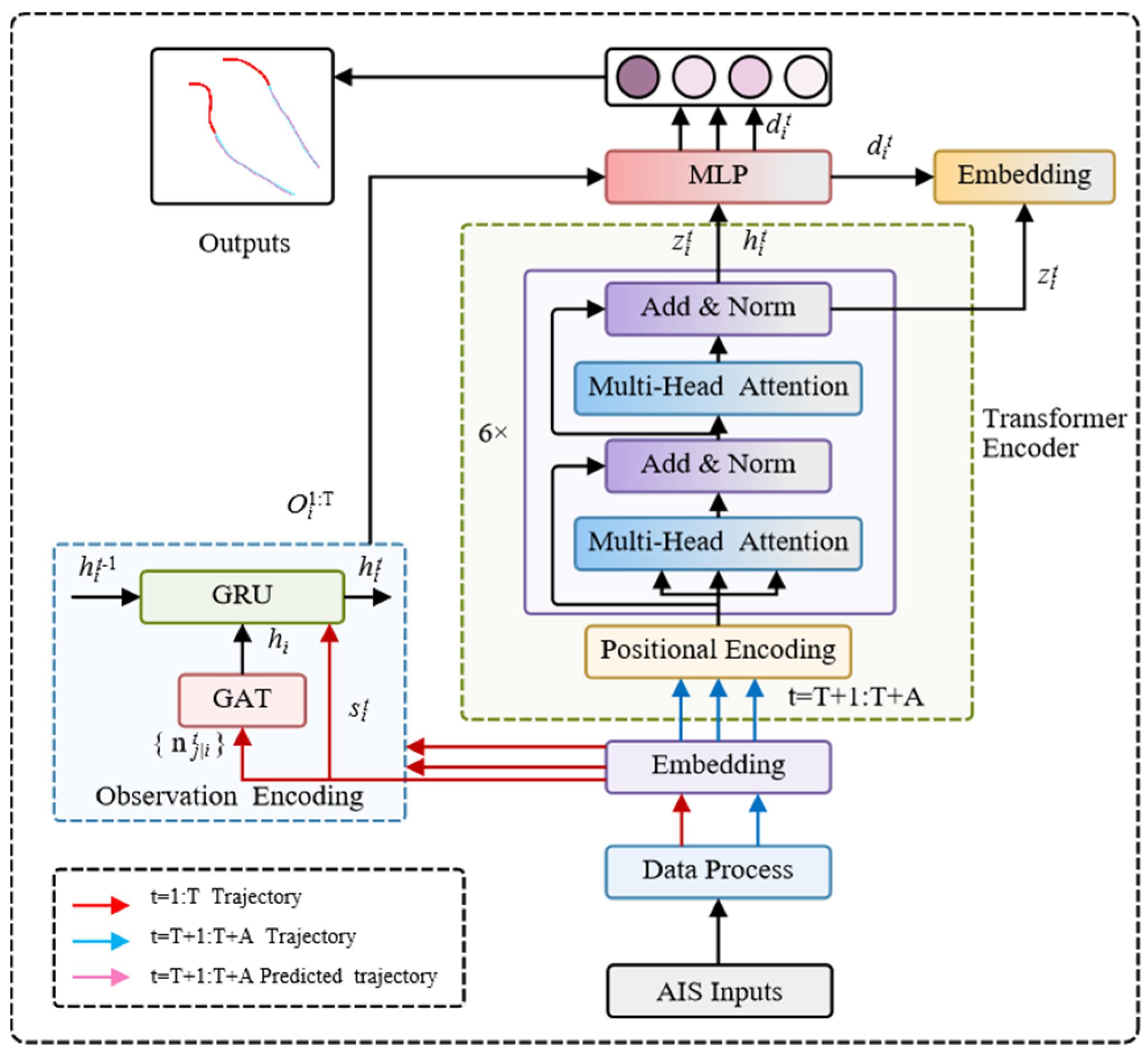
2.1. Model Architecture

Figure 2 shows a systematic overview of our model. The input data for this model consist of AIS data, which, after data processing, yield the trajectory data of ship i and its neighbors j. Assuming the scenario involves N ships, $x_i^t$ represent the two-dimensional coordinates of the i-th ship at time step t. After obtaining the trajectory data for the time range 1:T + A, the information of ship i and its neighbors j is fed into the embedding layer to obtain high-dimensionality data. The data corresponding to the time range 1:T are input into the observation encoder, while the data from T + 1:T + A are fed into the Transformer Encoder. The purpose of this model is not to directly predict the absolute coordinates $x_i^{T+1:T+A}$ but rather to generate a displacement sequence $d_i^{T+\mathrm{l}:T+A}=\left[d_i^{T+\mathrm{l}},d_i^{T+2},\dots ,d_i^{T+A}\right]$, where $d_i^{t+1}\triangleq x_i^{t+1}-x_i^t$.

Specifically, the input data, after passing through the observation encoder introduced in Section 2.2, yield the observation vector $O_i^{1:T}$, where $O_i^{1:T}$ represents the observation data sequence of ship i at time step t. Meanwhile, the target trajectory is fed into the Transformer Encoder, and to enhance the model’s capacity to capture complex dynamic trajectories, the latent variable $z_i^t$ is introduced at time step t to capture dependencies within the future trajectory sequence. The Transformer Encoder can be expressed as

$$H_i=\mathit{Transformer}\mathit{Encoder}({\psi }_{zd}(z_i^{1:T},d_i^{1:T}))$$

(1)

where ${\psi }_{zd}(·)$ represents the embedding neural network, for t = T + 1, …, T + A, with the calculation details provided in Section 2.3.

The latent variable $z_i^t$ is sampled as follows:

$$z_i^t~q_{\phi }(z_i^t|H_i^t,h_i^T)$$

(2)

where $q_{\phi }$ is a parameterized posterior distribution used to generate the latent variable $z_i^t$, which depends on the output $H_i^t$ of the Transformer Encoder and the historical observation encoding $h_i^t={\psi }_h(O_i^{1:T})$, where ${\psi }_h(·)$ is represented by an embedding neural network.

In summary, the generative formulation of this model is

$$p(d_i^{T+1:T+A}\mid O_i^{1:T})=\prod _{t=T+1}^{T+A}{\int }_{z_i^t}p(d_i^t\mid d_i^{T:t-1},O_i^{1:T},z_i^t)p_{\theta }(z_i^t\mid H_i^t)d{z}_i^t$$

(3)

In our baseline model, SocialVAE, the prior distribution depends on the RNN hidden state. In the proposed ShipTrack-TVAE, we replace the RNN with a Transformer, where the prior distribution depends on the output state $H_i^t$ of the Transformer Encoder. Here, $\theta$ represents the neural network parameters to be optimized. The outer $p(d_i^{T+1:T+A}|O_i^{1:T})$ denotes the joint probability distribution over the future displacement sequence $d_i^{T+1:T+A}$ given the observed data sequence $O_i^{1:T}$, representing the probability of generating the entire future trajectory conditioned on the observed history. Within this framework, the inner conditional probability $p(d_i^t|d_i^{T:t-1},O_i^{1:T},z_i^t)$ describes the probability of generating the displacement $d_i^t$ at time t, conditioned on the historical displacements $d_i^{T:t-1}$, the observed data $O_i^{1:T}$, and the current latent variable $z_i^t$, thereby capturing the sequential generation of future displacements while integrating both historical information and latent dynamics. Additionally, $p_{\theta }(z_i^t\mid H_i^t)$ represents the prior distribution of the latent variable $z_i^t$, conditioned on the output state $H_i^t$ from the Transformer Encoder, where θ denotes the neural network parameters optimized during training. This prior distribution enables the generation of the latent variable based on the global features extracted by the encoder.

The sampling of displacement $d_i^t$ depends on the latent variable $z_i^t$ and the output state $H_i^t$ of the Transformer Encoder, resulting in

$$d_i^t~p_{\xi }(·|z_i^t,H_i^t)$$

(4)

where $\xi$ represents the neural network parameters to be optimized. The two-dimensional coordinates $x_i^t$ of the ship can be obtained based on the definition of $d_i^t$ as follows:

$$x_i^t=x_i^T+{\displaystyle {\sum }_{\tau =T+1}^t{d}_i^{\tau }}$$

(5)

where $x_i^t$ represents the spatial position of the i-th ship at time step t.

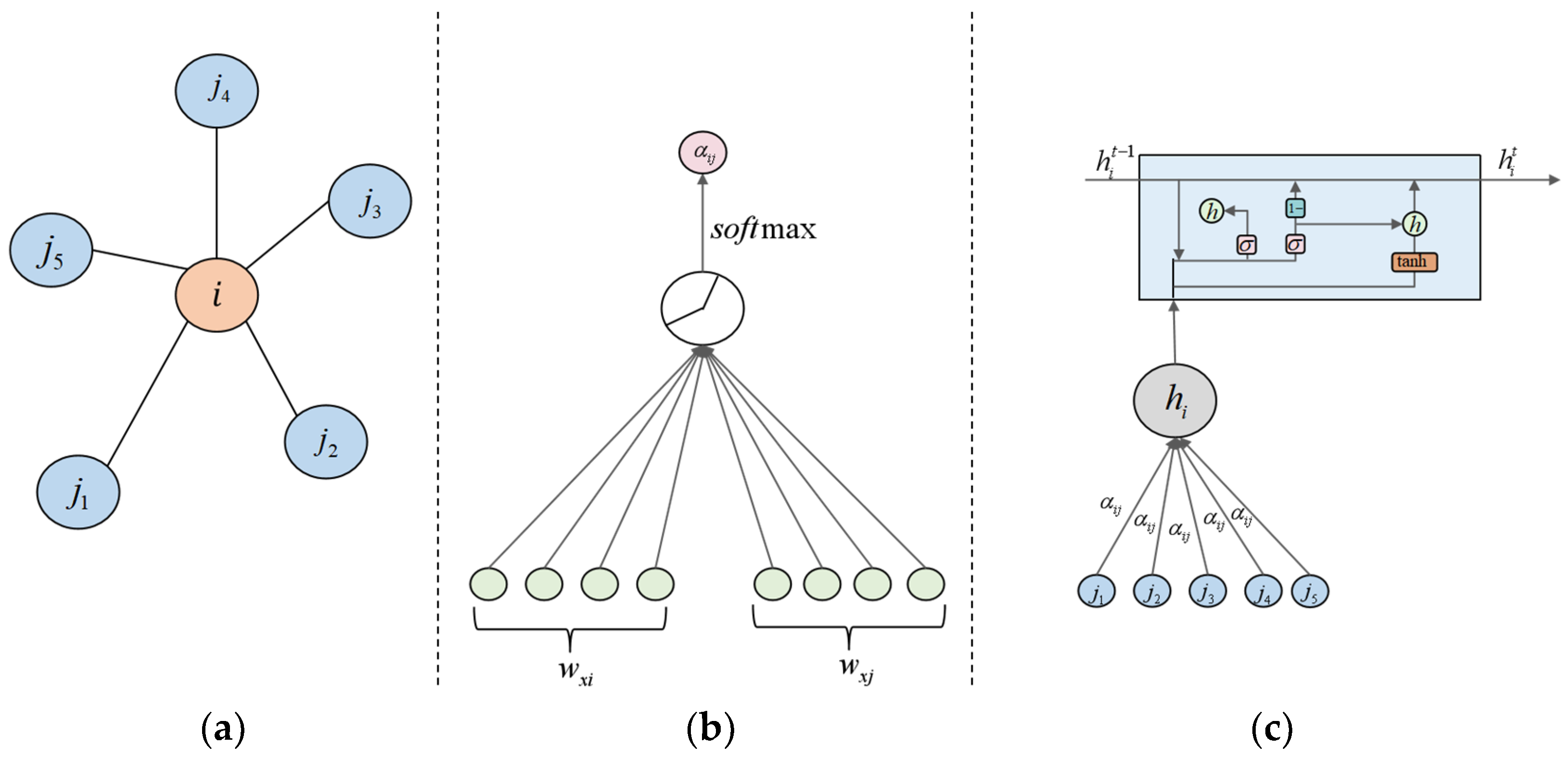
2.2. Observation Encoding

Figure 3 illustrates the main process of observation encoding. Figure 3a provides a schematic representation of a central ship i and its neighbor j. Figure 3b depicts the computation process of the graph attention mechanism. Figure 3c shows how the attention coefficient ${\alpha }_{ij}^t$, computed by a GAT, is applied to the feature representation of the neighboring ship, which is then passed to the GRU. The GRU integrates the fused neighbor ship features with its own features through the update and reset gates to capture dynamic changes between time steps. It outputs the updated hidden state, representing the encoding result at the current time step. The following sections provide a detailed explanation of the two steps.

First, a Graph Attention Network (GAT) is employed to process the neighboring nodes at each time step, generating feature representations for the neighbors. For a ship at time step t, the features of neighbor j are processed using the GAT to calculate the attention coefficient ${\alpha }_{ij}^t$, followed by a weighted summation:

$$e_{ij}^t=\mathrm{LeakyReLU}\left({\mathbf{a}}^T[W{n}_{ij}^t||W{s}_i^t]\right)$$

(6)

$${\alpha }_{ij}^t={\displaystyle \frac{\exp (e_{ij}^t)}{\sum _{k\in \mathcal{N}(i)}\exp (e_{ik}^t)}}$$

(7)

$$g_i^t=\sum _{j\in \mathcal{N}(i)}{\alpha }_{ij}^{t}W{n}_{ij}^t$$

(8)

where $n_{ij}^t$ represents the features of neighboring ship j relative to ship i, $s_i^t$ denotes the self-state of ship i, a is the learnable weight vector, and W is the linear transformation matrix. $e_{ij}^t$ represents the relationship strength between ship i and its neighbor j at time step t, processed through the LeakyReLU activation function. $g_i^t$ is the aggregated neighbor feature representation obtained through the GAT. In this process, Equation (7) calculates the attention score between the ship and its neighbors, Equation (8) normalizes this score to obtain the attention coefficient, and Equation (9) aggregates the features of the neighboring ships weighted by these coefficients, resulting in the final neighbor feature representation $g_i^t$.

The observation vector is formed by combining the self-state $s_i^t$ and the neighbor feature $g_i^t$ generated by the GAT, resulting in the observation vector $O_i^t$:

$$O_i^t=[f_s(s_i^t),g_i^t]$$

(9)

where $f_s$ is the function that processes the self-state. $O_i^t$ represents the observation vector of ship i at the current time step t, encompassing both the self-state and neighbor features.

The observation vector O serves as the output. At each time step t, the GAT generates the neighbor feature $g_i^t$, which is combined with the ship’s self-state $s_i^t$ to form the observation vector $O_i^t$. $O_i^t$ is the explicit output of the observation encoding module, representing the instantaneous observational information at the current time step, which is used by the decoder.

Time-series information is encoded (the GRU updates the hidden state): the GRU updates the observation vector $O_i^t$ and the hidden state $h_i^{t-1}$ from the previous time step to generate the hidden state $h_i^t$ for the current time step:

$$h_i^t=\mathrm{GRU}(O_i^t,h_i^{t-1})$$

(10)

where $h_i^{t-1}$ represents the hidden state from the (t − 1)-th time step. $h_i^t$ denotes the hidden state after the GRU update, containing historical information from the initial time step to the current time step.

h is the hidden state generated by the GRU at each time step, which is used for encoding historical time-series information. Although h is not an output, it is internally utilized to assist in generating the output at each time step. The primary role of h is to retain historical information and be updated at each time step by the GRU, thereby incorporating past information in the process of generating the output.

2.3. Transformer Encoder

This section elaborates on the Transformer Encoder part in Equation (2). The Transformer Encoder, with a structure consisting of 6 encoder layers, can better capture dependencies in long sequences and adapt to the complex trajectory sequences. The input sequence to the Transformer structure is

$$S={\left\{{\psi }_{zd}(z_i^t,d_i^t)\right\}}_{t-T+1}^{T+A}$$

(11)

where S represents the input sequence of target trajectory features, which contains the mapping of latent variables $z_i^t$ and displacement $d_i^t$ at each time step t, and H defines the number of the future sequences used for prediction. In the self-attention mechanism, the input sequence undergoes linear transformations to produce the query, key, and value matrices:

$$Q=S{W}_Q,K=S{W}_K,V=S{W}_V$$

(12)

where $W_Q$, $W_K$, and $W_V$ are linear transformation matrices that map the input S to the query (Q), key (K), and value (V), respectively. For each time step t, the self-attention mechanism captures the dependencies between time steps by calculating the attention weights among all time steps in the input sequence. The calculation formula is

$$Attention(Q,K,V)=softmax\left({\displaystyle \frac{Q{K}^T}{\sqrt{d_k}}}\right)V$$

(13)

where $Q{K}^T$ is the dot product of the query and key, representing the similarity between each time step, and $d_k$ is the scaling factor used to prevent the dot product value from becoming too large. The attention weights are then generated using the softmax function, and finally, a sum of attention weight is applied to obtain the context vector for each time step.

To enhance the model’s representation capability, the Transformer employs a multi-head attention mechanism, specifically configured with eight attention heads ($n_{head}=8$). That is, the query, key, and value matrices are split into multiple subspaces, and self-attention is independently computed in each subspace. Finally, the results are concatenated:

$$MultiHead(Q,K,V)=Concat(hea{d}_1,hea{d}_2,\dots ,heo{d}_k)W_O$$

(14)

where $hea{d}_i=Attention(Q{W}_Q^i,K{W}_K^i,V{W}_V^i),W_Q^i,W_K^i$, with $W_V^i$ denoting distinct projection matrices for the query, key, and value transformations, and $W_O$ is the linear transformation matrix for the output.

Each Transformer layer consists of two parts: a multi-head attention mechanism and a feed-forward neural network. Given an input S, the output $H^{(l)}$ of the l-th Transformer layer can be expressed as follows:

$$Z^{(l)}=MultiHead(H^{(l-1)},H^{(l-1)},H^{(l-1)})+H^{(l-1)}$$

(15)

where $FFN(Z^{(l)})=ReLU(Z^{(l)}{W}_1+b_1)W_2+b_2$

$$H^{(l)}=FFN(Z^{(l)})+Z^{(l)}$$

(16)

$$H^{(l)}=LayerNorm(H^l+FFN(Z^{(l)}))$$

(17)

After stacking 6 layers of the Transformer, the Transformer Encoder will output context $H_i$ from T + 1 to T + A time steps.

2.4. Decoder

This study replaces the RNN-based decoder with an MLP to handle feature generation tasks with shorter time steps more efficiently. While RNNs are advantageous for long sequences, their recursive structure introduces unnecessary computational overhead when processing short-time-step data. In contrast, the MLP processes the input in a single pass, providing higher efficiency and performance for short-sequence generation. Using an MLP simplifies the model’s complexity and improves both computational efficiency and training speed. Therefore, the decoder in this model adopts an MLP to better adapt to short-time-step generation tasks, maintaining model performance while reducing computational overhead.

The task of the decoder is to generate the target variable (e.g., the position of the ship) from the latent variable $z_i^t$ and hidden state $H_i^t$. To achieve this, we implement the decoder using a Multilayer Perceptron (MLP) structure.

At time step t, the input to the decoder consists of the latent variable $z_i^t$ and hidden state $H_i^t$, which are concatenated into a single vector:

$$inpu{t}_i^t=\left[z_i^t,H_i^t\right]$$

(18)

In the embedding layer, the decoder processes the input using a two-layer fully connected network (MLP) to obtain the intermediate representation ${xy}_i^t$:

$$x{y}_i^t=\mathrm{R}\mathrm{e}LU6(W_2\cdot \mathrm{R}\mathrm{e}LU6(W_1\cdot inpu{t}_i^t+{\mathrm{b}}_1)+{\mathrm{b}}_2)$$

(19)

where $W_1$ represents the weight matrix of the first layer, ${\mathrm{b}}_1$ is the bias vector of the first layer, $W_2$ is the weight matrix of the second layer, ${\mathrm{b}}_2$ is the bias vector of the second layer, and ReLU6 is a ReLU activation function used to limit the output in the range of [0, 6].

The final output of the decoder is computed using a linear layer to predict the ship’s position:

$$lo{c}_i^t=W_3\cdot x{y}_i^t+b_3$$

(20)

where $W_3$ is the weight matrix of the output layer, and $b_3$ is the bias vector of the output layer. Here, $lo{c}_i^t$ represents the position information generated at time step t.

The entire decoding process can be summarized as follows:

$$lo{c}_i^t=W_3·{\mathrm{R}\mathrm{e}\mathrm{L}\mathrm{U}6(\mathrm{W}}_2·{\mathrm{R}\mathrm{e}\mathrm{L}\mathrm{U}6(\mathrm{W}}_1·[{\mathrm{z}}_i^t,{\mathrm{H}}_i^t]+{\mathrm{b}}_1)+{\mathrm{b}}_2)+{\mathrm{b}}_3$$

(21)

This formula describes the entire process of generating the target variable from the latent variable ${\mathrm{z}}_i^t$ and the hidden state $H_i^t$.

2.5. Loss Function

The model introduces a reconstruction error, KL divergence, and collision loss. The reconstruction error measures the difference between the generated trajectory and the true trajectory. The formula is as follows:

$$\mathrm{R}\mathrm{e}c=\sum _{t=1}^T{∥x_t-{\mathrm{l}\mathrm{o}\mathrm{c}}_t∥}^2$$

(22)

where $x_t$ represents the true trajectory at the t-th time step, and ${\mathrm{l}\mathrm{o}\mathrm{c}}_t$ represents the generated predicted trajectory.

Before calculating KL divergence, we first introduce the concept of the standard normal distribution. The standard normal distribution PDF(z) is a special normal distribution with a mean of 0 and a variance of 1, used as the prior distribution for the latent variable. Its probability density function (PDF) is given by

$$PDF(z)={\displaystyle \frac{1}{\sqrt{2\mathrm{\Gamma }}}}\mathrm{e}\mathrm{x}\mathrm{p}(-{\displaystyle \frac{z^2}{2}})$$

(23)

KL divergence is used to measure the difference between the latent variable distribution q(z/x) and the standard normal distribution PDF(z) in generative models. The standard KL divergence formula is used as follows:

$$KL=-{\displaystyle \frac{1}{2}}\sum _{i=1}^N(1+\mathrm{l}\mathrm{o}\mathrm{g}({\sigma }^2)-{\mu }^2-{\sigma }^2)$$

(24)

where μ and σ are the mean and standard deviation of the latent variable, respectively.

In addition to reconstruction error and KL divergence, we also introduce collision loss into the model. This is designed to ensure that the predicted trajectory does not collide with neighboring agents. By calculating the distance between the predicted trajectory and neighboring agents, and ensuring that it is always greater than the set safety distance, we define the loss function as follows:

$$CollisionLoss=\sum _t\mathrm{l}\mathrm{o}\mathrm{g}({\displaystyle \frac{dis\mathrm{t}\mathrm{a}\mathrm{n}ces(s)}{d_{min}}})$$

(25)

where $dis\mathrm{t}\mathrm{a}\mathrm{n}ces(s)$ represents the distance between the predicted trajectory and neighboring agents at time step t. $d_{min}$ is the safety threshold, indicating the minimum safe distance that should be maintained between the predicted trajectory and neighboring agents to avoid collisions.

To enforce the constraint, the logarithmic term $\mathrm{l}\mathrm{o}\mathrm{g}({\displaystyle \frac{dis\mathrm{t}\mathrm{a}\mathrm{n}ces(s)}{d_{min}}})$ ensures that as the distance approaches $d_{min}$, the penalty increases significantly, discouraging trajectories that bring ships closer than the safe threshold. For cases where $dis\mathrm{t}\mathrm{a}\mathrm{n}ces(s)<d_{min}$, the loss contributes a significant penalty to the total function.

This loss is achieved by constraining the distance between the predicted agent and neighboring agents. When the distance is less than the safety threshold, the loss function value increases. The final total loss function integrates the reconstruction error (Rec), KL divergence (KL), and collision avoidance loss. It is defined as follows:

$$Loss=\mathrm{R}\mathrm{e}c+KL+\lambda \times CollisionLoss$$

(26)

where λ is a coefficient that controls the weight of the collision avoidance loss relative to the other loss terms.

3. Experimental Results and Analysis

3.1. Data Collection and Preprocessing

This study uses AIS ship data from The Navigation Guarantee Center of the South China Sea to ensure the reliability of trajectory prediction. The ships in the area mainly include commercial transport ships, passenger ferries, and fishing ships, as shown in Figure 4. The Qiongzhou Strait is one of the busiest waterways in China. The region has a large number of ships involved in various types of maritime traffic, making the AIS data from this area suitable for model prediction. We selected 8589 ships from June to September 2020. The longitude range is from 109.93 to 111.49, and the latitude range is from 19.92 to 20.31. The original AIS data were sourced from satellite–ground AIS stations in Qiongzhou Strait waterways. Due to partial data loss, inconsistencies, and other issues, we chose to preprocess the original AIS data. First, a comprehensive evaluation was conducted using actual ship trajectories based on AIS data. Typically, due to factors such as adverse weather conditions and limited communication channels, the collected raw AIS data contain a large amount of missing data, random noise, and outliers [27]. To overcome these issues, we applied a neural network to enhance the quality of AIS-based ship trajectory data [28]. In addition, to synchronize the AIS data, we directly applied cubic spline interpolation to interpolate the ship trajectories. The time interval between any two consecutive timestamps was set to 20 s. Finally, the dataset was split into the training and testing sets in an 8:2 ratio using the Holdout cross-validation method.

3.2. Network Parameter Setting

This study was conducted on a Windows 11 operating system using Pycharm as the programming software and Torch 1.11.0+cu113 as the deep learning framework, with Python 3.8.19. The Transformer, GAT, Softmax, GCNs and MLP models were all implemented using PyTorch 1.11.0. All experiments were performed on a 3.4 GHz Intel 14700 KF CPU and an NVIDIA RTX 4070 Ti Super GPU (16 GB RAM).

This section provides detailed network parameter settings for the ShipTrack-TVAE model. The model encodes the input ship coordinates into a 256-dimensional vector using an embedding layer. The observation radius (OB_NUMBER) is set to 5, representing the range of neighbors at each time step. The model also includes a Transformer Encoder composed of six Transformer layers, each containing eight attention heads to enhance the representation of spatial and temporal features.

During training, the Adam optimizer was used with an initial learning rate of 1 × 10⁻⁴. The learning rate decayed by a factor of 0.1 every 30 epochs to improve convergence. The batch size (BATCH_SIZE) was set to 64, and the model was trained for 100 epochs, with 100 batches per epoch. Early stopping based on the validation loss was employed, with a patience of 10 epochs to prevent overfitting. The training and validation datasets were split in an 8:2 ratio, and all batches were shuffled to ensure robustness. The minimum safety distance between ships was set to 1 nautical mile.

The hyperparameters of the model, including the learning rate, batch size, and the number of encoder layers, were tuned using a grid search approach. The final parameter settings were selected based on the validation performance and evaluated using metrics such as Average Displacement Error (ADE) and Final Displacement Error (FDE). The optimal settings were found to be a learning rate of 1 × 10⁻⁴, a batch size of 64, and six encoder layers.

Table 1. The parameter settings of ShipTrack-TVAE.

Parameters	Setting
The number of encoder layers	6
The number of multi-heads	8
Learning rate	0.0001
Batch size	64
Max epoch	100
Number of observed neighbors	5
Prediction horizon	35
Observation horizon	20

summarizes the main parameter settings of the model.

The main parameter settings of the model are shown in Table 1.

3.3. Evaluation Metrics and Comparison Baselines

In addition to adopting the Average Displacement Error (ADE) and Final Displacement Error (FDE) as evaluation metrics [29,30], this study also introduces ambient pressure error (APE) [31], an indicator used to assess the navigational safety of ships. These metrics are used to evaluate whether there is a risk of collision during the prediction process and the consistency of the predicted trajectory with the actual trajectory in terms of collision avoidance strategies. The use of these metrics ensures a fair and robust evaluation of the prediction results. ADE and FDE are defined as follows:

$$ADE={\displaystyle \frac{\sum _{n=1}^N\sum _{t=t_{obs}+1}^{t_{obs}+\mathrm{\Delta }t}{∥{\mathrm{l}\mathrm{o}\mathrm{c}}_i^t-x_i^t∥}_2}{N\times (\mathrm{\Delta }t-1)}}$$

(27)

$$FDE={\displaystyle \frac{\sum _{n=1}^N\parallel {\mathrm{l}\mathrm{o}\mathrm{c}}_i^t-x_i^t{\parallel }_2}{N}},t=t_{abs}+\mathrm{\Delta }t$$

(28)

where N represents the number of ships, and Δt represents the total time interval of the corresponding period.

$$APE=min\left(1,{\displaystyle \frac{1}{1080}}\sum _{i=-90}^{+90}SJL(\theta +i)\right)$$

(29)

where $SJL(\theta +i)$ is defined as

$$SJL(\theta +i)=\left(a\cdot {\displaystyle \frac{(d_i-R)}{v\cdot 1852}}\cdot 3600-3.82\right)\cdot \mathrm{c}\mathrm{o}\mathrm{s}\left({\displaystyle \frac{{\mathrm{bearing}}_i}{2}}\right)$$

(30)

where $SJL(\theta +i)$ represents the calculated ambient pressure at heading $\theta +i$, while APE denotes the averaged ambient pressure error over a ±90° range around the ship’s current heading. θ represents the current heading of the ship. $d_i$ denotes the distance between the navigating ship and a nearby target ship at heading $\theta +i$. R is the minimum safe distance to be maintained, calculated as $R=0.98\times L_{ship}+0.5\times L_{anchored}$, where $L_{ship}$ and $L_{anchored}$ represent the lengths of the navigating and anchored ships, respectively. $v$ refers to the speed of the navigating ship. $a$ is a regression coefficient related to the gross tonnage (GT) of the ship. ${\mathrm{bearing}}_i$ is the relative bearing of the obstacle or target ship with respect to the navigating ship. $\mathrm{c}\mathrm{o}\mathrm{s}\left({\displaystyle \frac{{\mathrm{bearing}}_i}{2}}\right)$ serves as a weighting factor that adjusts for the influence of obstacles or ships at different relative positions.

The comparison models used in this study include Bidirectional RNN (BiRNN) [32], LSTM [33], Seq2Seq [34], Social-STGCNN [35], and SocialVAE [19]. The Bidirectional Recurrent Neural Network (BiRNN) consists of two recurrent neural networks that process the input sequence in both forward and backward directions, thereby improving the reliability of time-series data prediction. The Long Short-Term Memory (LSTM) network is a recurrent neural network architecture designed to effectively capture long-term dependencies in sequential data. By using memory cells and specialized gating mechanisms, LSTM can retain and extract information over longer sequences. The Sequence-to-Sequence (Seq2Seq) model consists of an encoder–decoder framework and is commonly used for tasks such as machine translation and text generation. In this framework, the encoder encodes the input sequence into a fixed-length vector representation, which is then decoded by the decoder to generate the output sequence, allowing the model to handle variable-length input and output sequences. Social-STGCNN is a deep learning model specifically designed for trajectory modeling and prediction using Graph Convolutional Networks (GCNs) to integrate spatiotemporal information. SocialVAE is the baseline model of the proposed approach in this study. It is a generative model used for trajectory prediction that generates more accurate future trajectories by capturing interactions between individuals and their environment.

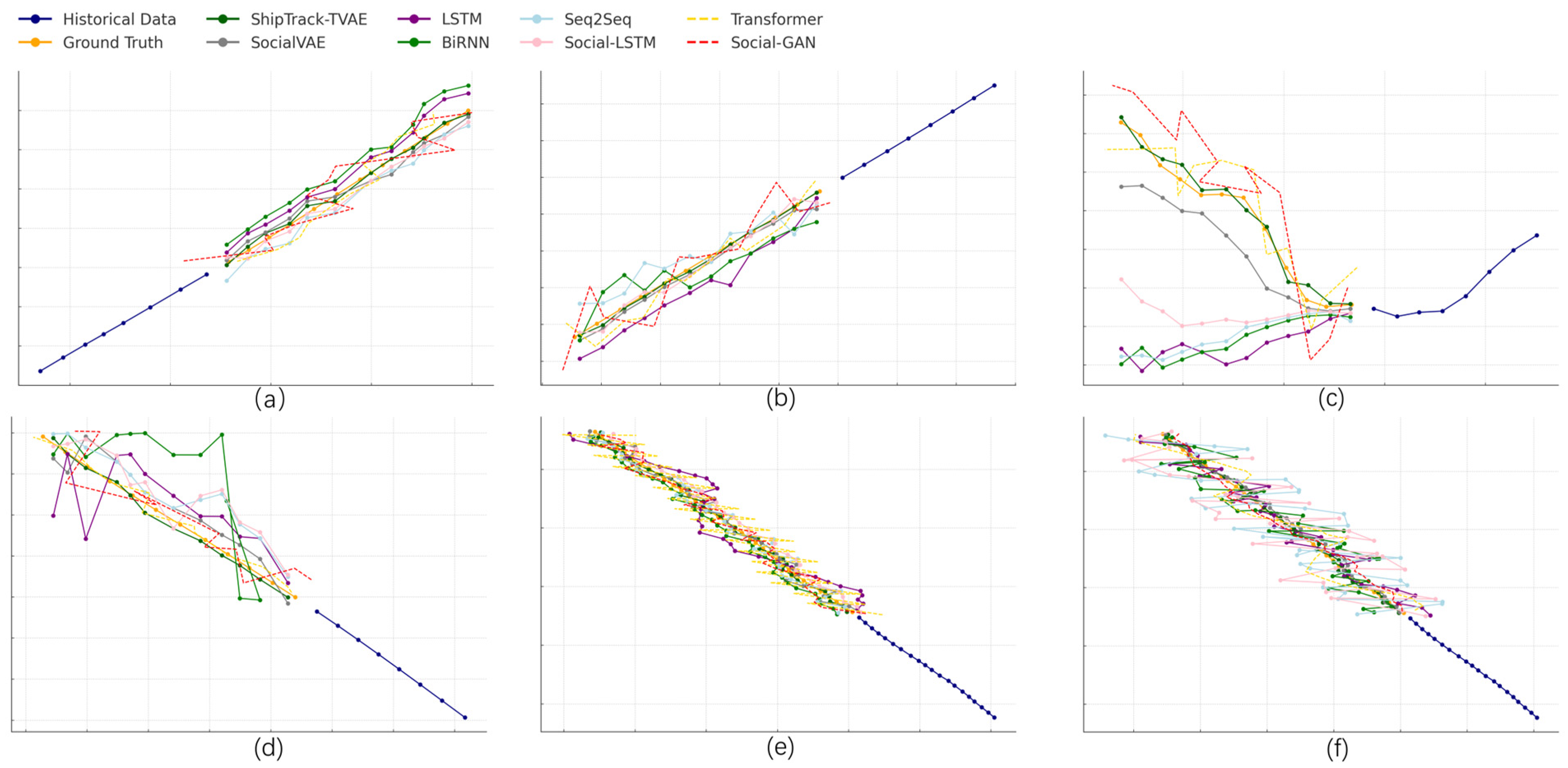
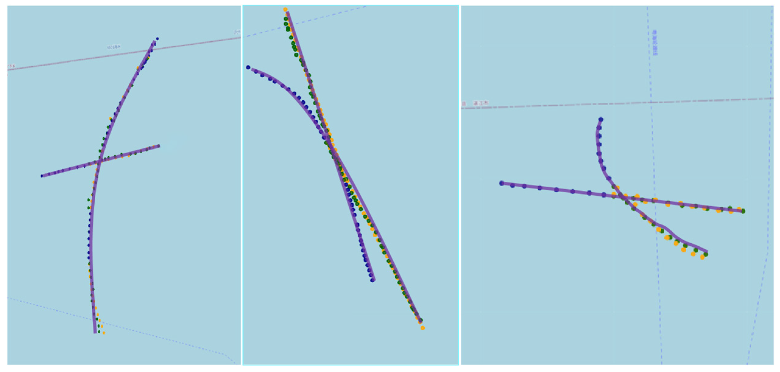
3.4. Comparative Test

The

Table 2. The average ADE and FDE values of different deep learning methods.

Step	Metrics	ShipTrack-TVAE	SocialVAE	BiRNN	LSTM	Seq2Seq	Social-STGCNN	Social-GAN	Transformer
12	ADE	0.0118	0.0135	0.183	0.0565	0.0328	0.0257	0.0437	0.0187
	FDE	0.0206	0.0249	0.234	0.146	0.774	0.0505	0.0955	0.0361
	APE	0.23	0.30	0.44	0.36	0.34	0.31	0.35	0.30
35	ADE	0.0275	0.0327	0.479	0.0931	0.0794	0.0564	0.0853	0.0381
	FDE	0.0423	0.0593	0.913	0.231	0.173	0.119	0.191	0.0693
	APE	0.24	0.32	0.46	0.39	0.36	0.34	0.38	0.33
80	ADE	0.0472	0.0604	0.583	0.265	0.168	0.135	0.212	0.0725
	FDE	0.0903	0.1099	1.234	0.596	0.474	0.505	0.563	0.1179
	APE	0.27	0.35	0.51	0.41	0.39	0.37	0.40	0.36

Note: ADE and FDE metrics are used to evaluate prediction results over hundreds of meters, where smaller values indicate greater prediction accuracy.

shows the comparative experiment on ship trajectory prediction conducted using the Hainan dataset. The results show that various algorithms effectively capture the interactions between ships, thereby reducing prediction errors. This result further demonstrates that considering interactions with other ships in the same navigable area is crucial for trajectory prediction in typical traffic scenarios. Compared to RNN variants and Seq2Seq methods, our proposed ShipTrack-TVAE method shows superior performance in capturing interactions between ships. The prediction accuracy of ShipTrack-TVAE on the Hainan dataset is superior to that of all comparison algorithms, particularly in long-term prediction.

The table shows the comparative experiment on ship trajectory prediction conducted using the Qiongzhou Strait dataset. The results indicate that all algorithms can capture interactions between ships to some extent, thereby reducing prediction errors. However, compared to other algorithms, ShipTrack-TVAE exhibits superior performance in ADE and FDE at each step, especially in long-term step prediction.

For 20-step predictions, ShipTrack-TVAE demonstrates significant improvements in Average Displacement Error (ADE), Final Displacement Error (FDE), and Average Position Error (APE) compared to other models. Specifically, ShipTrack-TVAE achieves an ADE and FDE improvement of 93.6% and 91.2%, respectively, compared to BiRNN, as well as an APE improvement of 47.7%. Compared with LSTM, the improvements in ADE, FDE, and APE are 79.1%, 85.9%, and 36.1%, respectively. Furthermore, ShipTrack-TVAE exhibits enhancements of 64.0%, 97.3%, and 32.4% in ADE, FDE, and APE over Seq2Seq, respectively, and 54.1%, 59.2%, and 28.1% over Social-STGCNN. ShipTrack-TVAE achieves ADE and FDE improvements of 73.0% and 78.4%, respectively, compared to Social-GAN, as well as an APE improvement of 34.3%. Compared to the Transformer, ShipTrack-TVAE provides more modest improvements of 36.9% and 43.0% in ADE and FDE, respectively, and a 23.3% improvement in APE. Compared with SocialVAE, ShipTrack-TVAE provides a more modest yet significant improvement of 12.6%, 17.3%, and 23.3% in ADE, FDE, and APE, respectively.

At 35 steps, the superiority of ShipTrack-TVAE becomes more evident across all three metrics. Specifically, ShipTrack-TVAE achieves ADE, FDE, and APE improvements of 94.3%, 95.4%, and 52.2% over BiRNN, respectively. Compared with LSTM, the improvements are 70.5%, 81.7%, and 38.5% in ADE, FDE, and APE, respectively. Against Seq2Seq, ShipTrack-TVAE demonstrates enhancements of 65.4%, 75.5%, and 33.3% in ADE, FDE, and APE, respectively, and 51.2%, 64.5%, and 29.4% over Social-STGCNN. Compared to Social-GAN, ShipTrack-TVAE achieves improvements of 67.7%, 77.9%, and 29.4% in ADE, FDE, and APE, respectively. Against the Transformer, ShipTrack-TVAE achieves ADE and FDE improvements of 27.8% and 38.9%, respectively, and a 9.1% improvement in APE. Relative to SocialVAE, improvements of 15.9%, 28.7%, and 25.0% are observed in ADE, FDE, and APE, respectively.

For 80-step predictions, ShipTrack-TVAE consistently outperforms alternative models, demonstrating substantial improvements across all metrics. Specifically, the improvements in ADE, FDE, and APE are 91.9%, 92.7%, and 47.1% compared with BiRNN, and 82.2%, 84.9%, and 30.8% compared with LSTM, respectively. Compared to Seq2Seq, ShipTrack-TVAE provides enhancements of 71.9%, 80.9%, and 30.8% in ADE, FDE, and APE, respectively, and 65.0%, 82.1%, and 27.0% in comparison with Social-STGCNN. ShipTrack-TVAE achieves ADE and FDE improvements of 77.7% and 82.0%, respectively, compared to Social-GAN, and a 25.9% improvement in APE. Compared to the Transformer, ShipTrack-TVAE achieves improvements of 34.8% and 23.4% in ADE and FDE, respectively, and a 7.4% improvement in APE. ShipTrack-TVAE also achieves ADE, FDE, and APE improvements of 21.9%, 17.9%, and 22.9% compared to SocialVAE, respectively.

These results clearly demonstrate that ShipTrack-TVAE achieves superior prediction accuracy across all prediction horizons, particularly excelling in long-term predictions. This performance underscores the significant potential and applicability of ShipTrack-TVAE in real-world scenarios, especially in contexts where accurate long-term trajectory predictions are crucial. The consistent improvements across all metrics, including ADE, FDE, and APE, validate the model’s capability to effectively capture complex interactions and accurately predict future ship trajectories, thereby enhancing maritime situational awareness and safety.

To evaluate the computational efficiency of ShipTrack-TVAE, training time and inference speed were measured under different prediction horizons (20, 35, and 80 steps). As shown in

Table 3. Computational efficiency metrics across different prediction steps.

Step	Metrics	ShipTrack-TVAE	SocialVAE	BiRNN	LSTM	Seq2Seq	Social-STGCNN	Social-GAN	Transformer
12	Training Time (s/epoch)	250	220	150	170	200	180	230	240
	Inference Speed (s/step)	0.016	0.013	0.010	0.011	0.012	0.010	0.012	0.014
35	Training Time (s/epoch)	290	250	170	190	230	200	260	280
	Inference Speed (s/step)	0.019	0.015	0.012	0.013	0.014	0.012	0.014	0.016
80	Training Time (s/epoch)	370	320	220	250	300	260	340	360
	Inference Speed (s/step)	0.024	0.020	0.015	0.016	0.018	0.015	0.018	0.021

, the ShipTrack-TVAE model requires 250 s per epoch for a prediction horizon of 20 steps, increasing to 370 s per epoch for 80 steps. The inference speed exhibits a similar trend, growing from 0.016 s per step to 0.024 s per step as the prediction horizon extends. These results align with the expected computational overhead introduced by the Transformer Encoder, which has a quadratic complexity in sequence length.

While ShipTrack-TVAE shows longer training and inference times compared to baseline models, the increase is justified by its significant improvement in accuracy. For example, at 80 steps, ShipTrack-TVAE reduces ADE and FDE by 21.9% and 17.9%, respectively, compared to SocialVAE. These findings demonstrate the trade-off between computational cost and accuracy, with ShipTrack-TVAE excelling in long-term trajectory predictions for complex maritime environments.

To objectively evaluate the trade-off between computational efficiency and prediction accuracy, we introduce a Comprehensive Performance Index (CPI). This metric incorporates both training time and inference speed, alongside accuracy metrics ADE and FDE. The CPI is defined as

$$CPI={\displaystyle \frac{InferenceSpeed}{TrainingTime\times ADE}}+{\displaystyle \frac{InferenceSpeed}{TrainingTime\times FDE}}$$

(31)

The results, as shown in Figure 5, demonstrate that ShipTrack-TVAE achieves the highest CPI values across different prediction horizons (12, 35, and 80 steps), as well as in the overall average CPI. Despite its relatively longer training time, ShipTrack-TVAE’s superior inference speed and remarkable accuracy enable it to outperform other models comprehensively.

Compared to models such as SocialVAE and the Transformer, ShipTrack-TVAE demonstrates a substantial advantage in the CPI, particularly for shorter prediction horizons like 12 steps, where its performance significantly outpaces other models. Although the gap in the CPI narrows as the prediction horizon extends, ShipTrack-TVAE consistently maintains a notable lead, showcasing its balanced combination of inference efficiency and superior accuracy. These results highlight ShipTrack-TVAE’s excellent performance across varying prediction steps, making it highly suitable for maritime trajectory prediction tasks.

3.5. Ablation Experiment

In this section, we describe ablation experiments that we conducted using the Qiongzhou Strait dataset to evaluate the impact of different modules on the overall performance of the ShipTrack-TVAE model. Specifically, we compared the prediction accuracy between the ShipTrack-TVAE and SocialVAE models and further analyzed the impact of the collision avoidance module on the ADE and FDE at different steps, as shown in

Table 4. The ablation study of ShipTrack-TVAE: ADE and FDE evaluation at different prediction steps.

Model	ADE (Step = 20)	FDE (Step = 20)	APE (Step = 20)	ADE (Step = 35)	FDE (Step = 35)	APE (Step = 35)	ADE (Step = 80)	FDE (Step = 80)	APE (Step = 80)
SocialVAE (Base)	0.0135	0.0249	0.30	0.0327	0.0593	0.32	0.0604	0.1099	0.35
Base + Transformer	0.0125	0.0225	0.29	0.0301	0.0516	0.30	0.0545	0.1001	0.33
Base + Transformer + Collision (Ours)	0.0118	0.0206	0.23	0.0275	0.0423	0.24	0.0472	0.0903	0.27

.

In the ablation experiment, incorporating the Transformer module significantly enhances the model’s prediction accuracy across different time steps. Specifically, for a step size of 20, the addition of the Transformer module reduces the ADE from 0.0135 in SocialVAE to 0.0125, representing an improvement of approximately 7.4%; the FDE decreases from 0.0249 to 0.0225, an improvement of approximately 9.6%; and the APE is reduced from 0.30 to 0.29, showing an improvement of approximately 3.3%. When the step size is 80, the ADE decreases from 0.0604 to 0.0545, representing an improvement of approximately 9.8%; the FDE decreases from 0.1099 to 0.1001, an improvement of approximately 8.9%; and the APE reduces from 0.35 to 0.33, an improvement of approximately 5.7%. These results demonstrate that the Transformer module is significantly advantageous in capturing the complex interactions between ships, further enhancing the accuracy of trajectory prediction.

Upon incorporating the collision avoidance module, the prediction accuracy of the ShipTrack-TVAE model further improves across different time steps. Specifically, for a step size of 20, the ADE improves by approximately 5.6%, the FDE improves by approximately 8.4%, and the APE improves by approximately 20.7%. For a step size of 35, the ADE improves by approximately 8.7%, the FDE improves by approximately 17.8%, and the APE improves by approximately 20.0%. For a step size of 80, the ADE improves by approximately 13.4%, the FDE improves by approximately 10.9%, and the APE improves by approximately 18.2%. These results clearly indicate that introducing the collision avoidance module significantly mitigates the potential collision risk between ships, particularly enhancing the accuracy of long-term predictions.

In the ablation study, varying the safety distance parameter $d_{min}$ demonstrates its significant impact on the accuracy and safety of ship trajectory predictions across different time steps. As shown in

Table 5. Ablation study of ShipTrack-TVAE: $d_{min}$ evaluation in different prediction steps.

${\mathit{d}}_{\mathit{m}\mathit{i}\mathit{n}}$ (Nautical Miles)	ADE (Step = 12)	FDE (Step = 12)	APE (Step = 12)	ADE (Step = 35)	FDE (Step = 35)	APE (Step = 35)	ADE (Step = 80)	FDE (Step = 80)	APE (Step = 80)
1	0.0118	0.0206	0.23	0.0275	0.0423	0.24	0.0472	0.0903	0.27
1.5	0.0121	0.0210	0.24	0.0280	0.0430	0.25	0.0480	0.0920	0.28
2	0.0125	0.0215	0.25	0.0288	0.0440	0.26	0.0492	0.0945	0.29
2.5	0.0130	0.0223	0.27	0.0300	0.0455	0.28	0.0508	0.0970	0.30
3	0.0138	0.0235	0.29	0.0315	0.0480	0.30	0.0528	0.1005	0.31

, as $d_{min}$ increases from 1 to 3 nautical miles, both ADE and FDE exhibit a gradual upward trend, indicating a slight decline in trajectory prediction accuracy. For example, when $d_{min}$ = 1, the ADE and FDE values for a step size of 80 are 0.0472 and 0.0903, respectively. These values increase to 0.0528 and 0.1005 for $d_{min}$ = 3, reflecting increases of approximately 11.9% and 11.3%. This trend is attributed to the model’s adherence to stricter safety constraints, which results in more conservative trajectory predictions. Meanwhile, the APE also shows a moderate increase across all time steps as $d_{min}$ grows, indicating heightened environmental pressure due to the additional maneuvering requirements imposed by larger safety margins. For instance, the APE rises from 0.27 at $d_{min}$ = 1 to 0.31 at $d_{min}$ = 3 for a step size of 80, representing an increase of 14.8%. These results highlight the trade-off between maintaining trajectory accuracy and enforcing stricter collision avoidance constraints.

The findings emphasize the importance of selecting an appropriate safety distance parameter based on operational requirements. Smaller $d_{min}$ values, such as 1 nautical mile, yield higher accuracy but may compromise safety by allowing closer proximity between ships. In contrast, larger $d_{min}$ values, such as 2.5 or 3 nautical miles, significantly enhance safety by reducing collision risks, as reflected in the lower APE values, but at the cost of increased prediction errors. This trade-off suggests that the optimal value of $d_{min}$ should balance the accuracy and safety requirements of the target application. Future research could explore adaptive safety distance mechanisms that dynamically adjust $d_{min}$ based on real-time traffic density and environmental conditions, further improving the model’s applicability to diverse maritime scenarios.

3.6. Analysis of Results

To qualitatively evaluate the performance of our proposed model, we generated visualizations of the prediction results across different scenarios and datasets, as shown in Figure 6. This study randomly selected six ship trajectories from the Qiongzhou Strait dataset for comparative experiments, and the visualization results are shown in Figure 6. When the trajectory is a straight line (e.g., Figure 6a,b,d–f), both the ShipTrack-TVAE model and the SocialVAE model obtain accurate prediction results. However, the SocialVAE model has difficulty predicting ship trajectories when the ships are turning or preparing to turn. In contrast, the ShipTrack-TVAE model demonstrates excellent performance due to its powerful spatiotemporal modeling capabilities (e.g., Figure 6c). The ShipTrack-TVAE model demonstrates the best prediction performance in terms of accuracy and robustness across different scenarios of the Qiongzhou Strait dataset. The high similarity between the predicted trajectories and the actual trajectories of the ships demonstrates that ShipTrack-TVAE considers the potential interactions between ships and has strong spatiotemporal modeling capabilities.

In addition, this study presents the distribution of ship trajectories predicted using ShipTrack-TVAE, as shown in Figure 7, Figure 8 and Figure 9. The trajectory distribution predicted by ShipTrack-TVAE is highly consistent with the actual sailing direction of the ships, further demonstrating the strong predictive capabilities of ShipTrack-TVAE in ship trajectory prediction tasks.

Figure 7 shows the result of predicting 12 frames from an 8-frame input for a total of 1000 ship trajectories. The time interval between each trajectory point is 20 s. The blue trajectory represents the true trajectory of the first 8 frames, the yellow trajectory represents the true trajectory of the subsequent 12 frames, and the green trajectory represents the 12 frames predicted by the model. The fit between the green predicted trajectory and the yellow true trajectory is high, indicating a good prediction effect when the step size is 12.

Figure 8 shows the result of predicting 35 frames from a 20-frame input for a total of 500 ship trajectories. The time interval between each trajectory point is also 20 s. The blue trajectory represents the true trajectory of the first 20 frames, the yellow trajectory represents the true trajectory of the subsequent 35 frames, and the green trajectory represents the predicted 35 frames. It is clear that the green and yellow tracks still show a good fit in the overall trend, indicating that ShipTrack-TVAE maintains high accuracy in prediction with a step size of 35.

Figure 9 shows the result of predicting 80 frames from a 40-frame input. This source contains 200 ship trajectories, and the time interval between trajectory points is also 20 s. The blue trajectory represents the true trajectory of the first 40 frames, the yellow trajectory represents the true trajectory of the subsequent 80 frames, and the green trajectory represents the predicted 80 frames by the model. In this figure, the green predicted trajectory and the yellow true trajectory are highly consistent in most instances, demonstrating the robustness and accuracy of ShipTrack-TVAE at a step size of 80, particularly when handling complex curved and straight paths.

The high degree of fit between the green predicted trajectories and the yellow true trajectories in these images, especially those of long-term predictions in Figure 9, demonstrates the significant potential of the ShipTrack-TVAE algorithm in trajectory prediction in complex navigation environments, highlighting the model’s excellent performance and robustness in medium- and long-term predictions.

To enhance the interpretability of the proposed ShipTrack-TVAE model, trajectory prediction visualizations are incorporated to illustrate its effectiveness in collision avoidance scenarios. These visualizations highlight the model’s capability to predict future trajectories while ensuring that the predicted paths adhere to defined safety constraints.

Figure 10a illustrates the scenario where the collision avoidance mechanism is enabled. In this case, the predicted trajectory (red line) maintains a safe distance from the neighboring ship’s trajectory (green line), as indicated by the safety zones (orange circles). This result demonstrates the model’s ability to dynamically adjust trajectories and mitigate collision risks. In contrast, Figure 10b depicts the scenario without collision avoidance. The predicted trajectory intersects with the safety zones, indicating potential collision risks due to the absence of trajectory adjustments. These visualizations highlight the critical role of the collision avoidance module in ensuring navigational safety.

To complement these results, Figure 11 provides a detailed visualization of ship interactions in the Qiongzhou Strait. The map illustrates the trajectories of multiple ships, with the center ship’s trajectory highlighted in red. The interaction region, marked by the red rectangle, highlights the critical moment when the center ship adjusts its trajectory to avoid collisions with nearby ships. By recognizing the spatial and temporal dynamics of surrounding ships, the model dynamically adjusts its trajectory, ensuring navigational safety. The identified interaction region showcases the proposed model’s effectiveness in reducing collision risks in highly congested maritime environments.

4. Conclusions

This study introduces a novel ship trajectory prediction model called ShipTrack-TVAE, which combines the powerful Transformer architecture with the SocialVAE framework. This model not only effectively captures the intricate spatiotemporal dependencies present in multi-ship interactions, but it also offers a nuanced approach to modeling the complex dynamics of maritime trajectories. The primary contributions of this work include the development of a hybrid model architecture that merges the strengths of the Transformer and SocialVAE and the addition of a dedicated collision avoidance module designed to enhance both the accuracy and safety of trajectory predictions in challenging navigational settings. The seamless integration of these components enables the model to simultaneously capture spatial and temporal interactions among ships, addressing significant challenges in multi-ship trajectory prediction and collision avoidance. Experimental evaluations validate the model’s effectiveness in multi-ship and multi-step prediction tasks, demonstrating notable improvements in accuracy, robustness, and adaptability compared to other advanced prediction methods. The superior performance of ShipTrack-TVAE highlights its potential ability to enhance maritime safety and decision-making processes in navigating and managing complex environments with high traffic density and variable ship behaviors. However, the AIS does not include hydrological conditions, meteorological influences, and waterway characteristics, which directly impact the trends of ship trajectories. Therefore, our proposed model has a limitation when facing a complex environment.

In the future, we will develop a multi-variant trajectory prediction model considering more impactful factors in complex environments, such as tides, currents, and wind. By integrating these multimodal data sources, we aim to develop a comprehensive framework to address dynamic and complex interactions in real-world maritime environments. Furthermore, leveraging our existing ship spatiotemporal big data platform, we plan to deploy and validate the ShipTrack-TVAE model under practical conditions. This platform, optimized for processing and visualizing large-scale AIS datasets in real time, will allow us to address challenges related to scalability and real-time application. Additionally, we plan to evaluate the model’s generalizability by testing it on datasets from diverse maritime regions, such as open oceans, estuaries, and inland waterways. This cross-regional validation will demonstrate the model’s adaptability to various conditions, improving its accuracy and robustness for different operational scenarios, particularly for autonomous and unmanned ships.

References

1. Lehtola, V.; Montewka, J.; Goerlandt, F.; Guinness, R.; Lensu, M. Finding safe and efficient shipping routes in ice-covered waters: A framework and a model. Cold Reg. Sci. Technol. 2019, 165, 102795. [Google Scholar] [CrossRef]
2. Felski, A.; Jaskólski, K.; Banyś, P. Comprehensive Assessment of Automatic Identification System (AIS) Data Application to Anti-collision Manoeuvring. J. Navig. 2015, 68, 697–717. [Google Scholar] [CrossRef]
3. Murray, B.; Perera, L.P. An AIS-based deep learning framework for regional ship behavior prediction. Reliab. Eng. Syst. Saf. 2021, 215, 107819. [Google Scholar] [CrossRef]
4. Dalsnes, B.R.; Hexeberg, S.; Flåten, A.L.; Eriksen, B.-O.H.; Brekke, E.F. The Neighbor Course Distribution Method with Gaussian Mixture Models for AIS-Based Vessel Trajectory Prediction. In Proceedings of the 2018 21st International Conference on Information Fusion (FUSION), Cambridge, UK, 10–13 July 2018; pp. 580–587. [Google Scholar] [CrossRef]
5. Zhang, X.; Liu, G.; Hu, C.; Ma, X. Wavelet Analysis Based Hidden Markov Model for Large Ship Trajectory Prediction. In Proceedings of the 2019 Chinese Control Conference (CCC), Guangzhou, China, 27–30 July 2019; pp. 2913–2918. [Google Scholar] [CrossRef]
6. Tang, H.; Yin, Y.; Shen, H. A model for vessel trajectory prediction based on long short-term memory neural network. J. Mar. Eng. Technol. 2022, 21, 136–145. [Google Scholar] [CrossRef]
7. Suo, Y.; Chen, W.; Claramunt, C.; Yang, S. A Ship Trajectory Prediction Framework Based on a Recurrent Neural Network. Sensors 2020, 20, 5133. [Google Scholar] [CrossRef]
8. Sun, Q.; Tang, Z.; Gao, J.; Zhang, G. Short-term ship motion attitude prediction based on LSTM and GPR. Appl. Ocean Res. 2022, 118, 102927. [Google Scholar] [CrossRef]
9. Zhang, X.; Fu, X.; Xiao, Z.; Xu, H.; Qin, Z. Vessel Trajectory Prediction in Maritime Transportation: Current Approaches and Beyond. IEEE Trans. Intell. Transp. Syst. 2022, 23, 19980–19998. [Google Scholar] [CrossRef]
10. Liu, Y.; Zhang, J.; Fang, L.; Jiang, Q.; Zhou, B. Multimodal Motion Prediction With Stacked Transformers. In Proceedings of the IEEE/CVF Conference on Computer Vision and Pattern Recognition (CVPR), Nashville, TN, USA, 20–25 June 2021; pp. 7577–7586. [Google Scholar] [CrossRef]
11. Jiang, D.; Shi, G.; Li, N.; Ma, L.; Li, W.; Shi, J. TRFM-LS: Transformer-Based Deep Learning Method for Vessel Trajectory Prediction. J. Mar. Sci. Eng. 2023, 11, 880. [Google Scholar] [CrossRef]
12. Qiang, H.; Guo, Z.; Xie, S.; Peng, X. MSTFormer: Motion Inspired Spatial-temporal Transformer with Dynamic-aware Attention for long-term Vessel Trajectory Prediction. arXiv 2023. [Google Scholar] [CrossRef]
13. Lin, Z.; Li, F.; Zeng, L.; Hao, J.; Pan, M. Ship trajectory prediction model based on improved SocialVAE. In Proceedings of the 5th International Conference on Computer Information and Big Data Applications, Wuhan China, 26–28 April 2024; Association for Computing Machinery: New York, NY, USA; pp. 1145–1149. [Google Scholar] [CrossRef]
14. Zhang, S.; Wang, L.; Zhu, M.; Chen, S.; Zhang, H.; Zeng, Z. A Bi-directional LSTM Ship Trajectory Prediction Method based on Attention Mechanism. In Proceedings of the 2021 IEEE 5th Advanced Information Technology, Electronic and Automation Control Conference (IAEAC), Chongqing, China, 12–14 March 2021; pp. 1987–1993. [Google Scholar] [CrossRef]
15. Zhang, J.; Wang, H.; Cui, F.; Liu, Y.; Liu, Z.; Dong, J. Research into Ship Trajectory Prediction Based on An Improved LSTM Network. J. Mar. Sci. Eng. 2023, 11, 1268. [Google Scholar] [CrossRef]
16. Cui, Z.; Pan, M.; Lin, Z.; Liu, Z. A GAN based multi-vessel trajectory prediction method. J. Dalian Marit. Univ. 2023, 49, 51–60. [Google Scholar] [CrossRef]
17. Wu, Y.; Yv, W.; Zeng, G.; Shang, Y.; Liao, W. GL-STGCNN: Enhancing Multi-Ship Trajectory Prediction with MPC Correction. J. Mar. Sci. Eng. 2024, 12, 882. [Google Scholar] [CrossRef]
18. Suo, Y.; Ding, Z.; Zhang, T. The Mamba Model: A Novel Approach for Predicting Ship Trajectories. J. Mar. Sci. Eng. 2024, 12, 1321. [Google Scholar] [CrossRef]
19. Xu, P.; Hayet, J.-B.; Karamouzas, I. SocialVAE: Human Trajectory Prediction using Timewise Latents. arXiv 2022. [Google Scholar] [CrossRef]
20. Gao, W.; Liu, J.; Zhi, J.; Wang, J. Improved SocialVAE: A Socially-Aware Ship Trajectory Prediction Method for Port Operations. In Proceedings of the 2023 2nd International Conference on Machine Learning, Cloud Computing and Intelligent Mining (MLCCIM), Hubei, China, 25–29 July 2023; pp. 420–424. [Google Scholar] [CrossRef]
21. Xu, B.; Wang, X.; Li, S.; Li, J.; Liu, C. Social-CVAE: Pedestrian Trajectory Prediction Using Conditional Variational Auto-Encoder. In Proceedings of the Neural Information Processing; Luo, B., Cheng, L., Wu, Z.-G., Li, H., Li, C., Eds.; Springer Nature: Singapore, 2024; pp. 476–489. [Google Scholar] [CrossRef]
22. Liu, Z.; Li, S.; Hao, J.; Hu, J.; Pan, M. An Efficient and Fast Model Reduced Kernel KNN for Human Activity Recognition. J. Adv. Transp. 2021, 2021, 2026895. [Google Scholar] [CrossRef]
23. Vaswani, A.; Shazeer, N.; Parmar, N.; Uszkoreit, J.; Jones, L.; Gomez, A.N.; Kaiser, Ł.; Polosukhin, I. Attention is All you Need. arXiv 2017, arXiv:1706.03762. [Google Scholar]
24. Yang, Z.; Dai, Z.; Yang, Y.; Carbonell, J.; Salakhutdinov, R.R.; Le, Q.V. XLNet: Generalized Autoregressive Pretraining for Language Understanding. arXiv 2019, arXiv:1906.08237. [Google Scholar]
25. Devlin, J.; Chang, M.W.; Lee, K.; Toutanova, K. BERT: Pre-training of Deep Bidirectional Transformers for Language Understanding. arXiv 2018. [Google Scholar] [CrossRef]
26. Xue, H.; Wang, S.; Xia, M.; Guo, S. G-Trans: A hierarchical approach to vessel trajectory prediction with GRU-based transformer. Ocean Eng. 2024, 300, 117431. [Google Scholar] [CrossRef]
27. Huang, Z.-T.; Luo, Y.; Han, L.; Wang, K.; Yao, S.-S.; Su, H.-X.; Chen, S.; Cao, G.-Y.; De Fries, C.M.; Chen, Z.-S.; et al. Patterns of cardiometabolic multimorbidity and the risk of depressive symptoms in a longitudinal cohort of middle-aged and older Chinese. J. Affect. Disord. 2022, 301, 1–7. [Google Scholar] [CrossRef]
28. Murray, B.; Perera, L.P. A dual linear autoencoder approach for vessel trajectory prediction using historical AIS data. Ocean Eng. 2020, 209, 107478. [Google Scholar] [CrossRef]
29. Pellegrini, S.; Ess, A.; Schindler, K.; van Gool, L. You’ll never walk alone: Modeling social behavior for multi-target tracking. In Proceedings of the 2009 IEEE 12th International Conference on Computer Vision, Kyoto, Japan, 21 September–4 October 2009; pp. 261–268. [Google Scholar] [CrossRef]
30. Alahi, A.; Goel, K.; Ramanathan, V.; Robicquet, A.; Fei-Fei, L.; Savarese, S. Social LSTM: Human Trajectory Prediction in Crowded Spaces. In Proceedings of the 2016 IEEE Conference on Computer Vision and Pattern Recognition (CVPR), Las Vegas, NV, USA, 27–30 June 2016; pp. 961–971. [Google Scholar] [CrossRef]
31. Inoue, K.; Hara, K.; Kaneko, M.; Masuda, K. Assessment of the Correlation of Safety between Ship Handling and Environment. J. Jpn. Inst. Navig. 1996, 95, 147–153. [Google Scholar] [CrossRef]
32. Schuster, M.; Paliwal, K.K. Bidirectional recurrent neural networks. IEEE Trans. Signal Process. 1997, 45, 2673–2681. [Google Scholar] [CrossRef]
33. Wang, X.; Li, S.; Cao, Y.; Xin, T.; Yang, L. Dynamic speed trajectory generation and tracking control for autonomous driving of intelligent high-speed trains combining with deep learning and backstepping control methods. Eng. Appl. Artif. Intell. 2022, 115, 105230. [Google Scholar] [CrossRef]
34. Forti, N.; Millefiori, L.M.; Braca, P.; Willett, P. Prediction oof Vessel Trajectories from AIS Data via Sequence-to-Sequence Recurrent Neural Networks. In Proceedings of the ICASSP 2020–2020 IEEE International Conference on Acoustics, Speech and Signal Processing (ICASSP), Barcelona, Spain, 4–8 May 2020; pp. 8936–8940. [Google Scholar] [CrossRef]
35. Mohamed, A.; Qian, K.; Elhoseiny, M.; Claudel, C. Social-STGCNN: A Social Spatio-Temporal Graph Convolutional Neural Network for Human Trajectory Prediction. In Proceedings of the 2020 IEEE/CVF Conference on Computer Vision and Pattern Recognition (CVPR), Seattle, WA, USA, 13–19 June 2020; pp. 14412–14420. [Google Scholar] [CrossRef]
Figure 1. The SocialVAE model.
Jmse 12 02233 g001
Figure 2. The ShipTrack-TVAE model.
Jmse 12 02233 g002
Figure 3. The architecture of observation encoding. (a) Shows the connection between node i and its 5 neighboring nodes j, representing the neighbor selection process in GAT. (b) Illustrates the calculation of attention weights between node i and each neighbor j, followed by normalization using Softmax. (c) Demonstrates how the weighted neighbor information is transmitted to node hi and then passed into a GRU for further processing.
Jmse 12 02233 g003
Figure 4. Illustration of AIS data collection area from Qiongzhou Strait.
Jmse 12 02233 g004
Figure 5. Comparison of CPI across models.
Jmse 12 02233 g005
Figure 6. The visualization prediction results of comparison experiments on ship trajectory. (a) Predicted trajectory of the next 12 points for a ship navigating towards the upper right. (b) Predicted trajectory of the next 12 points for a ship navigating towards the lower left. (c) Predicted trajectory of the next 12 points for a ship turning towards the upper left. (d) Predicted trajectory of the next 12 points for a ship navigating towards the upper left. (e,f) Predicted trajectory of the next 35 points for a ship navigating towards the upper left.
Jmse 12 02233 g006
Figure 7. The prediction results in the Qiongzhou Strait with a step size of 12. The blue trajectory represents the input ship’s trajectory, the green trajectory represents the predicted ship’s trajectory, and the yellow trajectory represents the true ship’s trajectory.
Jmse 12 02233 g007
Figure 8. The prediction results in the Qiongzhou Strait with a step size of 35. The blue trajectory represents the input ship’s trajectory, the green trajectory represents the predicted ship’s trajectory, and the yellow trajectory represents the true ship’s trajectory.
Jmse 12 02233 g008
Figure 9. The prediction results in the Qiongzhou Strait with a step size of 80. The blue trajectory represents the input ship’s trajectory, the green trajectory represents the predicted ship’s trajectory, and the yellow trajectory represents the true ship’s trajectory.
Jmse 12 02233 g009
Figure 10. Comparison of trajectory predictions: with and without collision avoidance. (a) represents the predicted trajectory with the collision avoidance mechanism incorporated, and (b) represents the predicted trajectory without the collision avoidance mechanism.
Jmse 12 02233 g010
Figure 11. Visualization of ship interactions and collision avoidance in the Qiongzhou Strait. The blue trajectory represents the input ship’s trajectory, the green trajectory represents the predicted ship’s trajectory, and the yellow trajectory represents the true ship’s trajectory. The purple trajectory represents the ship’s navigation route.
Jmse 12 02233 g011