The Use of Air Pressure Measurements Within a Sealed Moonpool for Sea-State Estimation ^†

Abstract

To assess the viability of locations for wave energy farms and design effective coastal protection measures, knowledge of local wave regimes is required. The work described herein aims to develop a low-cost, self-powering wave-measuring device that comprises a floating buoy with a central moonpool. The relative motion of the water level in the moonpool to the buoy will pressurise and depressurise the air above the water column. The variation in air pressure may then be used to estimate the sea-state incident upon the buoy. Small-scale proof of concept tank testing was conducted at a 1:20 scale and at a larger 1:2.4 scale before a full-scale prototype was deployed at the Smartbay test site facility in Galway Bay, Ireland. A number of techniques by which full-scale sea states may be estimated from the pressure spectrum are explored. A successful technique, based on the average of multiple linear squared magnitude of the transfer functions obtained under different wave regimes is developed. The applicability of this technique is then confirmed using validation data obtained during the full-scale sea trials. While the technique has proven useful, investigation into potential seasonal bias has been conducted, and suggestions for further improvements to the technique, based on further calibration testing in real sea states, are proposed.

1. Introduction

Measurement of ocean waves plays a crucial role in understanding and determining wave energy resources, for example, to assess the viability of locations for wave energy farms. Furthermore, knowledge of local wave regimes is required for the design of effective coastal protection measures. While it may be possible to estimate expected waves at various locations, for example, using software developed by Delft University of Technology such as SWAN (Version 41.51), actual field measurements are required to both validate these estimates as well as offer insights into the sea state at locations where accurate models may not be easily constructed [1]. There are various systems and methods available for the measurement of local wave climates. Such methods include seabed pressure sensors, acoustic current profilers, radar (land-based and satellite), and surface-following buoys [2].

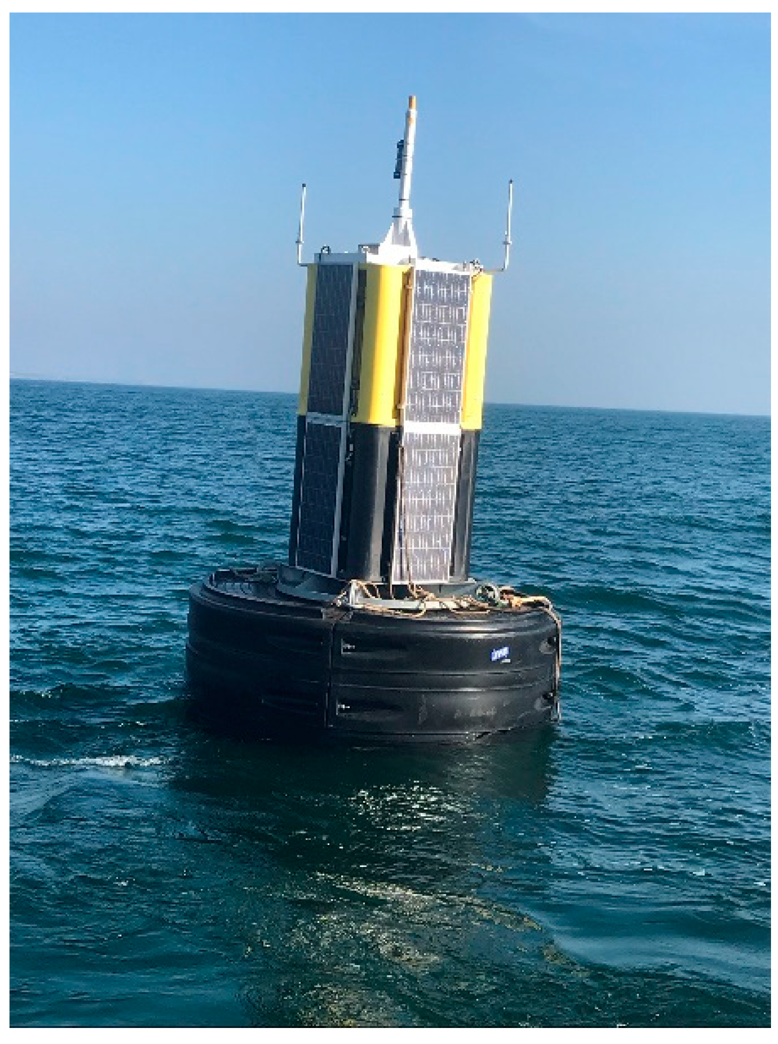
The work described in this paper has been undertaken as part of a phased project with the aim of developing a low-cost, wave-powered buoy to measure wave conditions to meet the needs of both developers and local authorities, named the Wave-Activated Sensor Power Buoy (WASP). A number of such low-cost buoys may potentially be deployed at a location to measure the local wave climate both temporally and spatially. Although the ultimate goal is for the WASP to be powered by a turbine driven by an Oscillating Water Column (OWC) to support data acquisition, this study primarily focuses on measuring variations in air pressure above the water column to estimate wave spectra and assess sea state conditions.

Section 2 of this paper describes the current state-of-the-art of wave measurement techniques. In Section 3, the development and construction of the full-scale WASP prototype is outlined. Section 4 presents the theory required to generate the squared magnitude of the transfer functions between the pressure in the moonpool and the incident sea state, as applied to the data obtained during sea trials. In Section 5, indicators of the general performance buoy are presented. Next, the results obtained for the linear squared magnitude of the transfer function between the sea state and the pressure are described. Finally, the estimated sea states obtained by applying the proposed technique to validation data are presented.

2. Review of Ocean Condition Monitoring and Wave Measurement

A number of methods are used to monitor and measure ocean conditions; in this section, the most common approaches are outlined.

2.1. Seabed Pressure Sensor-Based Measurements

Seabed pressure sensors are devices designed to measure the pressure at various depths in the ocean. These sensors play a crucial role in oceanographic research, environmental monitoring, and various industrial applications such as oil exploration. Seabed pressure sensors are typically placed on the ocean floor and are designed to withstand the harsh conditions of the marine environment. They operate based on the principle that pressure increases with depth in a fluid, such as seawater. These sensors convert the pressure exerted by the water column above them into electrical signals, which can then be transmitted to the surface or stored for later retrieval. From the variation in sub-surface pressure, the wave regime above a sensor can be estimated. The effectiveness of such sensors decreases as water depth increases [2].

2.2. Acoustic Doppler Current Profiler (ADCP)

An Acoustic Doppler Current Profiler (ADCP) is a device used to measure the velocity of water currents in oceans, rivers, and other water bodies. It employs the Doppler effect to determine the velocity of water particles along the acoustic beams emitted by the device. An ADCP emits acoustic beams (pulses of sound waves) into the water. When these beams encounter moving particles (such as water molecules or suspended sediments), the frequency of the sound waves is altered due to Doppler shift. The ADCP measures the change in frequency caused by the Doppler effect and uses this information to calculate the velocity of water particles at different depths. The device can produce and receive signals from multiple directions and can be stationary or mounted to a moving vehicle. Because the emitted signal extends down through the water column, it measures the current at many different depths and can determine the speed and direction of the varying currents within the water column, including the surface of the ocean. The water velocities, as determined from each beam, are combined and processed to produce a time series of the 3D wave-induced water velocities, and from that, the directional wave spectrum can be obtained [3].

2.3. Land-Based Radar

Land-based, high-frequency, surface wave radar is a rapidly emerging technology suitable for ocean wave remote sensing through line-of-sight wave measurement. The transmitted signals of coherent radar have all predefined phase angles to a reference, and this leads to the capability of obtaining the Doppler information due to changes in phase. Analysis of coherent microwave radar data usually involves the application of a 3D fast Fourier transformation (FFT) to the acquired backscatter images of the ocean area in order to estimate the spectra. Subsequently, wave parameters can be deduced based on a spectral analysis of the estimated spectra [4].

2.4. Satellite Radar

Satellite radar for ocean wave measurement utilises synthetic aperture radar (SAR) technology. SAR instruments on satellites transmit microwave signals towards the Earth’s surface and receive the backscattered signals. By analysing the returned signals, the satellite can generate images and data related to the ocean surface, including wave characteristics. Advantages of this system include providing a global perspective and allowing for the monitoring of waves over vast ocean areas. This is particularly useful for studying open-ocean wave patterns [5].

2.5. Data Buoys

Data buoys are floating platforms equipped with various sensors and instruments designed to collect and transmit data about the ocean and atmospheric conditions. These buoys play a crucial role in oceanography, meteorology, and climate research. Data buoys are typically equipped with a variety of sensors to measure parameters such as sea surface temperature, air temperature, humidity, barometric pressure, wind speed and direction, wave height, and ocean currents. There are different types of buoys, including moored buoys (anchored to the ocean floor), drifting buoys (free-floating and drifting with ocean currents), and profiling buoys (capable of moving vertically through the water column to collect profile data) [6].

2.5.1. Drifting Buoys

Drifting buoys are oceanographic instruments designed to collect and transmit various types of data while drifting with ocean currents. These buoys play a crucial role in monitoring and studying the dynamic properties of the world’s oceans. Drifting buoys provide real-time data on oceanic parameters such as sea surface temperature, salinity, and atmospheric conditions. This information is valuable for weather forecasting, climate research, and understanding oceanic trends. These devices are designed to move with ocean currents, allowing them to cover large areas. This mobility makes them suitable for studying ocean circulation patterns, including the tracking of currents and eddies. They are often more cost-effective than maintaining a fixed network of oceanographic instruments. They can cover vast expanses of the ocean at a relatively lower cost compared to deploying and maintaining fixed buoys or research vessels. These buoys are used in international programs, providing global coverage for data collection. This is particularly important for understanding large-scale oceanic processes and phenomena. Drifting buoys can be equipped with various sensors to measure different oceanic and atmospheric parameters. This versatility allows scientists to customize the buoys for specific research objectives. Drifting buoys can be deployed for extended periods, allowing for long-term monitoring of ocean conditions. This is crucial for detecting trends and changes in oceanic parameters over time [7].

2.5.2. Surface-Following Wave Measuring Buoys

Surface-following wave-measuring buoys, often referred to as wave buoys or wave sensors, are devices designed to measure and monitor ocean surface waves. Conventional wave regime measurement buoys work by ‘following’ the free surface of the ocean [8]. The onboard accelerometers measure the acceleration of the buoy, and the displacement of the buoy is then determined from the double integration of the accelerometer data. Hence, the time series of the motion of the buoy can be obtained by assuming the motion of the buoy matches the free surface elevation, and the wave spectrum at the deployment site may be estimated.

These buoys play a crucial role in collecting data on wave height, period, and direction and can provide information for various applications such as weather forecasting, climate research, and offshore engineering. Wave buoys are a well-established technology that can provide accurate and reliable measurements of wave characteristics, including wave height, period, and direction. This information is essential for understanding ocean dynamics and predicting extreme weather events. Many surface-following buoys are equipped with telemetry systems that enable real-time data transmission. This allows researchers and meteorologists to monitor wave conditions promptly and respond to changes in the environment. Wave buoys are designed to withstand harsh marine conditions, allowing for long-term deployment in open ocean environments. This durability ensures a consistent and continuous data stream for extended periods. These buoys can be deployed in various locations, including remote and deep-sea areas, providing a comprehensive understanding of wave patterns on a global scale. Wave buoys are often part of a broader ocean monitoring system and can be integrated with other sensors to measure parameters such as sea surface temperature, salinity, and atmospheric conditions. This integrated approach enhances the overall understanding of ocean dynamics [9]. However, such buoys are costly.

2.5.3. Waverider Buoy

The Waverider buoy, which was positioned c.400 m from the WASP during sea trials and was the data source for existing comparable sea-state conditions for this research, is an advanced oceanographic instrument used to measure wave properties, such as height, period, and direction, with high precision. The buoy is typically spherical or discus-shaped and designed to float on the water’s surface, anchored to the seafloor to maintain position. It is equipped with sensitive motion sensors, including accelerometers and gyroscopes, to detect its vertical and horizontal movements as it responds to wave-induced forces. These movements are analysed to derive wave energy, frequency, and direction. An important characteristic of the Waverider buoy is its natural frequency, which is carefully designed to be much higher than the wave frequencies it measures. This ensures that the buoy faithfully follows the wave motion without introducing significant distortion, allowing for accurate data collection. The processed wave data are transmitted in real-time via radio, satellite, or cellular systems to onshore stations, supporting applications in marine research, navigation, and offshore operations.

2.5.4. Pitch–Roll–Heave Buoys

Pitch–roll–heave buoys are disc-shaped buoys that follow the slope of the sea surface, as opposed to tracking the orbital motion like the particle-following buoys discussed in the previous section. The pitch and roll inclinations are measured along with the vertical heave. By combining these three measurements, an accurate picture of the free surface displacement can be obtained [10,11].

2.5.5. Innovation of the Research

The innovation of the research lies in utilizing air pressure variations above the water column to estimate wave spectra and sea-state conditions in the frequency domain, offering a novel, potentially less expensive and less power-consuming approach to wave analysis compared to traditional in-water measurement methods.

3. Description of the Full-Scale WASP Prototype

3.1. Background

Conventionally, the measurement of air pressure in an OWC (Oscillating Water Column) was crucial for understanding and optimizing the performance of WECs, which harness the energy from ocean waves [12]. However, while it is the intention that the WASP ultimately be powered by an OWC-driven turbine to provide power for data acquisition, this work focuses on the measurement of the variation in air pressure above the water column with a view to estimating wave spectra and sea state conditions.

The WASP comprises a floating body with a central moonpool. The relative motion of the water level in the moonpool to the buoy will pressurise and depressurise the air above the water column. It is intended that the air flows generated by the change in pressure will, in the final design of the device, be used to drive a unidirectional turbine in the manner of a conventional OWC device, which, in turn, will be used in conjunction with a generator to recharge an onboard battery pack. It is intended that once the WASP has been suitably calibrated, the wave spectrum may be estimated from measurements of the pressure of the air above the water column by determining a relationship between the incident wave spectrum and the pressure spectrum within the OWC chamber. Important statistical parameters relating to the sea state, such as the significant wave height and zero-cross period, may then be estimated from the spectral moments of the estimated wave spectrum. The WASP concept has been investigated through tank testing of a 1:20 scale model at Dundalk Institute of Technology [13] and a 1:2.4 scale model at the LIR National Ocean Test Facility, Ireland.

3.2. WASP Construction and Deployment

The initial full-scale prototype of the WASP used a modified, off-the-shelf buoy, the ‘Seagull’ navigation buoy manufactured by JFC Manufacturing Company Ltd., Tuam, Ireland [14], and was tested at the BlueWise Marine and Renewable Energy test site off the West Coast of Galway, Ireland [15]. The purpose of the prototype was to obtain data to explore the process of using the time series of the pressure in the air trapped above the water column (which is sealed from the atmosphere) to estimate sea-state parameters in the real world at full scale. To this end, the device was deployed at a location where the wave regime is independently measured by a Waverider surface-following buoy [15] at the BlueWise Marine test site. The prototype is not wave-powered; instead, batteries are recharged using six 80 W solar panels, and the air chamber above the water column is intentionally sealed from the atmosphere in order to maximise pressure in the chamber. It should be noted that the ‘Seagull’ buoy is not generally intended to be deployed in this configuration. A schematic of the Seagull buoy as configured during the full-scale testing is presented in Figure 1.

The prototype was deployed in February 2019 at the Marine Institute Galway Bay observatory and successfully recorded and transmitted data daily until its recovery in June 2019. A photograph of the WASP as deployed is shown in Figure 2. The test site allows for less exposed trials of smaller-scale ocean energy devices and those at an earlier stage of development. WASP was moored at a single point to a previously established single mooring system specifically installed for the WASP. The test site is located approximately 1.2 km off the Galway coastline and approximately 400 m from the location of an existing Irish Marine Institute Waverider data buoy.

Unlike wave-following buoys, the operational principle of the WASP depends on the interaction of the WASP with the ocean waves in order to pressurise and depressurise the air above the water column; the WASP does not operate on a wave-following basis. The time series of the pressure in the air volume above the water column was measured, recorded, and sampled at 8 Hz. This means that, in accordance with the Nyquist Limit [16], the WASP may be used to measure a pressure signal containing frequencies from 4 Hz and above. The WASP was retrieved in July 2019, having successfully uploaded 24 h of uninterrupted data each day for the duration of the deployment. During the deployment, the WASP was subject to a wide range of weather and sea state conditions and, from a robustness perspective, had survived and recorded data from the most severe winter storms of that year, including storms Gareth and Hannah, both of which brought wind gusts in excess of 130 km/h. The deployment resulted in the acquisition of several months of pressure signal readings from two Keller piezo-resistive differential pressure sensors [17]. Of these sensors, one covers a relatively low range of pressures at a relatively high resolution between +/−200 millibar. The other sensor operates between +/−1 bar with lower resolution and was included in order to capture extreme pressure events. For further details on the design and construction of the full-scale prototype WASP, please refer to [18].

4. Applied Theory

Single-input, single-output (SISO) systems play a crucial role in engineering and science, particularly in the analysis of dynamic systems where a single variable, acting as the input, influences one corresponding output. In such systems, the behaviour of the output is analysed with respect to changes in the input. SISO models are widely employed in control systems, signal processing, and environmental modelling, including the study of ocean wave energy. To provide a robust analysis, random data assumptions are often employed, particularly in the context of stationary and ergodic processes [19]. Under ideal conditions, the output of the system shown in Figure 3 is given by the convolution integral:

$$y\left(t\right)={\int }_0^{\infty }h\left(\tau \right)x\left(t-\tau \right)d\tau$$

(1)

where h($\tau$) = 0 for $\tau$ < 0 when the system is physically realisable.

where

$x\left(t\right)$ represents the stationary input

$y\left(t\right)$ represents the output

$h\left(t\right)$ represents the impulse response of the system

$X\left(f\right)$ represents the Fourier transform of $x\left(t\right)$

$Y\left(f\right)$ represents the Fourier transform of $y\left(t\right)$

$H\left(f\right)$ is the frequency-dependent, Fourier transfer function between $X\left(f\right)$ and $Y\left(f\right)$

$H\left(f\right)$ is the Fourier transform of $h\left(t\right).$

In random data analysis, particularly when dealing with environmental phenomena such as ocean waves, the assumption of stationarity is critical. A stationary process is one whose statistical properties, such as the mean, variance, and autocorrelation, remain constant over time. For example, in a SISO ocean wave energy system, if wave height is treated as the input and the energy extracted as the output, assuming stationarity simplifies the analysis by allowing the use of time-invariant models. An ergodic process, on the other hand, allows the use of time averages to represent ensemble averages, which is critical for practical analysis. In essence, ergodicity implies that a single realization of a process over a sufficiently long period contains all the statistical information needed to describe the system. For a SISO system, this is important because it means that long-term measurements of input–output behaviour can be treated as representative of the entire system.

Assuming that the input x(t) to the system in Figure 3 is a sample record from a stationary (ergodic) random process {x(t)}, the response y(t) will also belong to a stationary (ergodic) random process {y(t)}. Therefore, from Equation (1), the product y(t)y(t + τ) is given by the following:

$$y\left(t\right)y\left(t+\tau \right)={\int }_0^{\infty }{\int }_0^{\infty }h\left(\xi \right)h\left(\eta \right)x\left(t-\xi \right)x\left(t+\tau -\eta \right)d\xi d\eta$$

(2)

Taking the expected values of both sides of Equation (2) yields the input/output autocorrelation relation:

$$R_{yy}\left(\tau \right)={\int }_0^{\infty }{\int }_0^{\infty }h\left(\xi \right)h\left(\eta \right)R_{xx}\left(\tau -\xi -\eta \right)d\xi d\eta$$

(3)

Similarly, the product x(t)y(t + $\tau$) is given by

$$x\left(t\right)y(t+\tau )={\int }_0^{\infty }h\left(\xi \right)x\left(t\right)x\left(t\right)x\left(t+\tau -\xi \right)d\xi$$

(4)

Here, the expected values of both sides yield the input/output cross-correlation relation:

$$R_{xy}\left(\tau \right)={\int }_0^{\infty }h\left(\xi \right)R_{xx}\left(\tau -\xi \right)d\xi$$

(5)

Note that Equation (5) is a convolution integral of the same form as Equation (1). Direct Fourier transforms of Equations (3) and (5) after various algebraic steps yield two-sided spectral density functions $S_{xx}\left(f\right)$, $S_{yy}\left(f\right)$, and $S_{xy}\left(f\right)$, which satisfy important formulas. Equation (6) is called the input/output autospectrum relation, whereas Equation (7) is called the input/output cross-spectrum relation.

$$S_{yy}\left(f\right)=\left|H\right(f){|}^2{S}_{xx}\left(f\right)$$

(6)

$$S_{xy}\left(f\right)=H\left(f\right)S_{xx}\left(f\right)$$

(7)

In the work described herein, the measured time series of air pressure in the OWC is the input signal, $x\left(t\right)$, and the time series of surface water elevation of the incident sea state is the output signal $y\left(t\right)$. The two-sided auto-spectral density functions of the pressure data from the prototype WASP and the measured incident wave height data from the Waverider buoy are herein termed $Sxx\left(f\right)$ and $Syy\left(f\right)$, respectively. Thus, following from Equation (6), the squared magnitude of the transfer function between the pressure in the prototype WASP OWC and the incident sea state can be derived from the following equation:

$$|H\left(f\right){|}^2={\displaystyle \frac{S_{yy}\left(f\right)}{S_{xx}\left(f\right)}}$$

(8)

It is common in the field of oceanography to assume that free surface elevation at a point can be modelled as a stationary and ergodic process over the time frame of 20 to 30 min; this convention is followed in the current work.

5. Results

In this section, a number of key performance metrics are first included to demonstrate the behaviour of the WASP. Next, typical time series pressure results are illustrated before the results obtained in the frequency domain for the squared magnitude of the transfer function between the OWC and the free surface elevation are presented. Finally, a comparison between the significant wave height and zero crossing period obtained by the wave rider and those estimated using the squared magnitude of the average transfer function described herein for validation data, which were not used to generate the squared magnitude of the transfer function, are presented. The full range of sea states experienced by the WASP during the deployment can be found in the Supplementary Excel Spreadsheet available from the link provided at the end of this paper.

5.1. Performance Results

Data were recorded uninterrupted at a rate of 8 Hertz and uploaded from the WASP to the Microsoft Azure cloud service every 24 h [20]. The data included pressure signals from the sealed chamber above the water column in the OWC, air temperature within the day marker, and battery voltage. Figure 4 shows the variation in battery voltage over the course of a typical 24 h period corresponding to 21 April 2019. In Figure 5, the internal temperature of the day marker is shown over the same 24 h window. While battery and temperature monitoring may not be required for wave estimation, the information is useful for monitoring the WASP’s performance.

Note the 24 h period from which data are illustrated in Figure 4 was a relatively overcast day, and as the cloud covering cleared, an increase in battery voltage can be seen. Similarly, in Figure 5, an increase in the temperature as the day progressed can be seen. There were no issues with regard to temperature throughout the duration of deployment. Furthermore, the battery voltage never dropped below a point to impede stable operation.

5.2. Raw Pressure Results

An example of a typical time series of pressure recording from the 200 mbar pressure sensor for the same day shown in Figure 4 and Figure 5 is shown in Figure 6.

5.3. Frequency Domain Results

As previously noted, the time series of the pressure data within the OWC chamber was continuously recorded for the duration of the deployment of the WASP. Data from the Waverider wave following buoy at the BlueWise Marine test site for the corresponding time period were provided by the Marine Institute of Ireland. Note that the two devices were located approximately 400 m apart within the observatory for the duration of the deployment. In this work, it is assumed that the sea states experienced by both buoys are identical throughout. The operational frequency range of the Waverider buoy is 0.025–0.60 Hz. The mean Hs and Tz values for the test site are 0.8 m and 4 s, respectively.

The prototype WASP time series pressure data are transformed to the frequency domain using Welch’s Method [21]. In Figure 7, a typical wave spectrum for the Galway Bay test site, as recorded by the Waverider buoy, is presented.

Figure 8 presents the power density spectrum of the pressure signal from within the OWC chamber of the WASP for the corresponding half-hour time period.

In order to generate a single squared magnitude of the transfer function, the use of which can be subsequently verified, the data gathered during the deployment were divided into training data and validation data. The training dataset comprised data obtained during the month of March, while the remaining data from the months of April, May, and June were used as validation data.

In order to produce the squared magnitude of the transfer function from the training data, the power density spectrum of the WASP pressure signal was obtained for each half-hour of the training data. The squared of the magnitude of the linear transfer function between the power density spectrum of the WASP and the wave spectrum as measured by the Waverider buoy for each half hour was then obtained in accordance with Equation (8). In Figure 9, the squared of the magnitude of the transfer function for each half hour of the training data is presented.

As can be seen in Figure 9, a large number of the squared magnitude of the transfer functions is obtained, and variance between them is observed. In order to obtain a single squared magnitude of the transfer function, the average of the square amplitude of the transfer function at each frequency is taken. Such an approach may ultimately result in values at some frequencies that are lower than expected, as not all wave spectra will contain information at all frequencies. However, the results presented in Section 5.4 demonstrate the usefulness of such an approach. The final average squared amplitude of the transfer function is presented in Figure 10.

5.4. Sea Spectrum and Parameter Estimation

In this section, two sample wave spectra, as estimated by the WASP and measured by the Waverider, are first presented. Subsequently, the results obtained for key spectral parameters for the entire validation data are presented.

Figure 11 illustrates an example where there is a close match between the wave spectra as estimated by the WASP and as measured by the Waverider. Taking a random half-hour sample from the WASP data and comparing its power density spectrum against that of the Waverider for the same half-hour sample, reasonably satisfactory results are achieved, as can be seen.

However, not all random samples selected yielded the same level of accuracy. In Figure 12, while the WASP spectrum generally reflects that of the Waverider, there is a noticeable difference in the PSD at a frequency of 0.1 hertz. It should be noted again that the Waverider and full-scale prototype WASP were some 400 m from one another during the testing campaign.

When defining sea states, it is common to refer to a measure of the wave height, typically the significant wave height, Hs, and a measure of time, commonly the zero-crossing period, Tz. These parameters can be obtained from a wave spectrum using spectral moments as given in Equations (9) and (10).

$$H_s=4\sqrt{m_0}$$

(9)

$$T_z={\displaystyle \frac{m_1}{m_0}}$$

(10)

The average of the squared magnitude of the transfer function using the training data for March was applied to the WASP data for April, May, and June to generate an estimated wave spectrum for each half-hour. Spectral moments were then obtained for both the wave spectrums estimated by the WASP and measured by the Waverider. These spectra were then used to obtain estimates for Hs and Tz values for every half-hour sample for both devices for each month within the validation dataset. Figure 13 and Figure 14 present a comparison between the Hs and Tz values thus obtained for each half-hour segment in the month of June 2019.

As can be clearly seen for Hs in Figure 13, a strong correlation exists between the results obtained by the Waverider and those estimated by the WASP. It can be seen that the correlation for Tz is not strong; this may be in part due to the distance between the two buoys and a potential shoaling effect on the waves. However, a correlation between the two sets of Tz does exist.

5.5. Seasonal Bias

A squared magnitude of the transfer function obtained from frequency domain data is reflective of the frequencies contained within the sea states. Not all sea states will contain information at all applicable frequencies. Furthermore, it is possible that certain frequencies may dominate the sea state during specific times of the year to the exclusion of other frequencies. A squared magnitude of the transfer function obtained from the average of multiple squared magnitude of the transfer functions from a specific time of year may thus potentially contain seasonal bias. The results presented thus far in this paper are based on using the average of the squared magnitude of the transfer function for the month of March. In order to explore the potential for ‘seasonal bias’ within the confines of the available dataset, the averages of the squared magnitude of the transfer functions are compiled for the month of June and separately for the months of March, April, and May combined. Both of these averages of the squared magnitudes of the transfer functions are then used to estimate the significant wave height for June in conjunction with the pressure data from the WASP. In Figure 15, the estimated values for Hs for the month of June, obtained using the squared magnitude of the average transfer function for June in conjunction with the pressure data for June itself, are presented.

In Figure 16, the combined squared magnitude of the average transfer function for the months of March, April, and May is applied to the June pressure data to again estimate Hs for June.

Table 1. Correlation between Waverider and WASP Hs values and the RMS of the errors between the Hs values using varying averages of the squared magnitudes of the transfer functions.

avgTF Applied	March	June	March/April/May
Correlation %	97.4	97.699	97.796
RMS error	0.2293	0.3117	0.219

presents the correlation between the estimated Hs values and those obtained by the Waverider. The root mean square (RMS) of the error between the measured and estimated Hs values normalised by the RMS of the Hs values for the month of June as measured by the Waverider for each of the squared magnitudes of the transfer functions used in Figure 13, Figure 15 and Figure 16 are also presented. The RMS of the Hs values, as measured by the Waverider for the month of June, was 0.6185 m.

As can be seen in Table 1, the correlation between the estimated and measured values in all cases is in excess of 97%. However, it is in the magnitude of the significant wave height that any seasonal bias would be expected to manifest. A significant variation can be seen between the RMS of the error values for March and June while using a squared magnitude of the transfer function for three months appears to have the effect of smoothing out the seasonal variation. This dataset would initially appear to suggest the possibility of seasonal bias; however, additional data are required to confirm such a bias.

5.6. Piecewise Linear Squared Magnitude of the Transfer Function

In order for the use of the squared magnitude of the transfer function, such as that used herein, to be valid, the processes involved must be linear. However, air compression takes place, albeit to a small degree, within the chamber above the sealed moonpool; such compression may not be linear [22]. In order to explore the importance of such non-linearities, a piecewise [20] squared magnitude of the transfer function was developed based on the RMS of the pressure signal. It is assumed that the higher the RMS of the pressure signal, the more energetic the sea state. For the March dataset, the maximum pressure achieved within the chamber was identified. Five evenly sized pressure bands were established based on the maximum pressure measured for the month, and each half-hour segment of data was assigned to a pressure band based on the RMS for the pressure of that half-hour. A squared magnitude of the transfer function was then produced for each pressure band based on the average of the squared magnitude of the transfer functions for the data segments within that band. This results in five squared magnitude of the transfer functions, which are illustrated in Figure 17.

In order to apply the piecewise squared magnitude of the transfer functions to estimate Hs for the month of June, the RMS of the pressure signal for each segment in June is first determined, and the squared magnitude of the transfer function for the band in which that pressure lies is applied to that segment. Thus, a different squared magnitude of the transfer function is applied to different segments of the June data based on the RMS of the pressure signal in a given segment. The results of this process are presented in Figure 18.

The correlation between Hs obtained using the piecewise squared magnitude of the transfer functions and the Waverider was 97.99%, and the RMS error of the Hs value obtained from the piecewise squared magnitude of the transfer function was 0.216, as discussed in Section 5.5. This shows some improvement in the values obtained, for example, based only on the March squared magnitude of the transfer function of 0.2293; however, whether such an improvement is significant is debatable.

6. Discussion and Conclusions

As can be seen in Figure 13, Figure 14, Figure 15 and Figure 16, analysis of the data established that bulk statistics for the sea states, such as Hs and Tz, can be estimated from measured time domain pressure data. The initial results from this analysis are positive, with a correlation between spectra and Hs and Tz values in the order of 97% and with normalised RMSE values for Hs between 0.219 and 0.3117. In some instances, there are deviations between the values for Hs and Tz obtained from the WASP and those obtained from the Waverider. One source of this deviation may be the distance between the wave rider and the WASP, which were separated by approximately 400 m. Such deviations could also arise due to the use of an average of the squared magnitude of the transfer function, which is itself constructed from multiple squared magnitude of the transfer functions that individually may not contain information throughout the entire range of frequencies of interest. For example, comparing the wave spectra presented in Figure 11 and Figure 12, it can be seen that the spectrum illustrated in Figure 12 does not contain waves at frequencies in excess of 0.4 hertz (unlike that in Figure 11). As a result, the squared magnitude of the transfer function for the spectrum in Figure 12 will also not contain information beyond 0.4 hertz, and this adversely affects the accuracy of the overall average of the squared magnitude of the transfer function beyond this frequency. It should be noted that the testing campaign took place during the spring and summer months of 2019, and hence, the WASP operated in relatively benign sea states. Longer testing durations are desirable in order to capture seasonal variations, a wider range of sea states, and more extreme sea states typical of winter months.

In order to further refine the accuracy of the estimations of Hs and Tz from the WASP, a number of improvements to the WASP design and subsequent data analysis techniques are proposed.

The process of creating a suite of squared magnitude of the transfer functions based on discrete pressure bands, whereby the average of the squared magnitude of the transfer function for each pressure band is created from the squared magnitude of the transfer functions for data segments within that band (as illustrated in Figure 17 and described in Section 5.6), appears to show improvement in the estimation of Hs on simply using a single, averaged, squared magnitude of the transfer function. The results presented herein are based on data garnered over a four-month period from March to June 2019, with March data used for training purposes and April, May, and June data used for validation. If data were available for a longer period of time, the WASP would be subject to more sea states; this, in turn, would result in a greater range of pressures to assign to the pressure bands. The width of the pressure bands could be reduced, and the overall accuracy within each band could be improved due to the larger number of individual squared magnitudes of the transfer functions available for each band. Such data could be obtained through future deployments at the test site.

The squared magnitude of the transfer functions illustrated in Figure 9, Figure 10 and Figure 17 are created from the average of multiple squared magnitude of the transfer functions based on half-hour sea states. As discussed previously, an individual squared magnitude of the transfer function will not necessarily contain information at all frequencies within the possible range that may be experienced at that location. If the buoy was not excited at a particular frequency for a particular sea state, the magnitude of the resultant squared magnitude of the transfer function at that frequency would be minimal or zero for that sea state. Such values will affect the accuracy of the averaged squared magnitude of the transfer function. Future work will investigate a minimum magnitude for the squared magnitude of the transfer function at each frequency for each sea state before the results for that frequency for that sea state are included in the average of the squared magnitude of the transfer function. This process would also benefit from an increased amount of data, which would arise from further deployments at the test site.

The Seagull buoy was chosen to form the basis of the initial prototype as it was available off-the-shelf at the time of testing. The Seagull, however, is not designed to exhibit strong frequency responses in the range typically encountered in Irish coastal waters. As a result, the amplitude of the air pressure measured in the OWC chamber during the testing is relatively low. A suitable redesign of the buoy and water column could allow the device to be excited to a greater degree over the full range of frequencies likely to be experienced (and hence measured) at such locations. This could be achieved by ensuring the natural frequencies in modes of motion that will result in pressure changes, such as the piston mode of the water column and the heave mode of the buoy, are distinct but fall within the range of frequencies contained within the expected sea states. Such a redesign would result in higher amplitude signals in the desired frequency range, improving the signal-to-noise ratio and, hence, the accuracy of the estimates.