The Parameterization of the Sound Speed Profile in the Sea of Japan and Its Perturbation Caused by a Synoptic Eddy

Abstract

This study presents the description of the parameterization of sound speed distribution in the Sea of Japan in the presence of a synoptic eddy. An analytical representation of the background sound speed profile (SSP) on its periphery is proposed. The perturbation of sound speed directly associated with the presence of an eddy is investigated. The proposed parameterization of the background SSP leads to a Sturm–Liouville problem for normal mode computation, which is equivalent to the eigenvalue problem for the Schrödinger equation with the Morse potential. This equivalence leads to simple analytical formulae for normal modes and their respective horizontal wavenumbers. It is shown that in the presence of an eddy causing moderate variations in sound speed, the standard perturbation theory for acoustic modes can be applied to describe the variability in horizontal wavenumbers across the area in which the eddy is localized. The proposed parameterization can be applied to the sound propagation modeling in the Sea of Japan.

1. Introduction

The dependence of the sound speed on depth determines the conditions for sound propagation in the ocean, the interference structure of an acoustic field, and the shape of the impulse response function of the deep-water sound fixing and ranging channel (SOFAR, also known as deep sound channel) [1,2]. This dependence has been the subject of experimental and theoretical research since the discovery of the guided propagation of acoustic waves in the SOFAR in the 1950s. Since the sound speed profiles (SSPs) obtained in the course of direct measurements are often inconvenient for theoretical studies, a number of different analytical parameterizations for such profiles have been proposed [3,4,5,6], e.g., the canonical Munk profile [1,3]. The respective formulae often catch the properties of real dependencies of sound velocity on depth in different areas of the ocean, reasonably providing a useful simplification for sound propagation modeling.

Hydrological inhomogeneities of various kinds, including, e.g., internal waves, ocean fronts, and synoptic eddies, that are ubiquitous in the marine environment [7,8,9,10], can be considered a perturbation of an SSP averaged over a certain area (hereafter called the background SSP). Acoustical thermometry experiments [11,12,13] also led to the necessity of estimating the influence of eddy on sound propagation. This influence was investigated in several works [9,10,14,15,16,17,18], and some numerical models were proposed to handle eddy-induced propagation effects [19,20].

Although the effect of various hydrodynamical inhomogeneities on sound propagation in the ocean has been studied extensively throughout the past three decades, little information on the internal structure of synoptic eddies is available in acoustic literature. This study examines a cruciform section of a stable anticyclonic eddy observed in the Sea of Japan during the summer of 1999, aiming at the construction of an analytical model of the latter in the context of underwater acoustics (i.e., seen as a large-scale perturbation of the background SSP in the area).

The uniqueness of the dataset under consideration consists in the fact that a research vessel managed to pass approximately through the eddy center along both parallel and meridian while performing CTD downcasts every 20 km and acquiring vertical distributions of temperature and salinity. Using the collected data, we determined both the background sound velocity profile and its three-dimensional perturbation associated with the presence of the eddy. We also showed that the Morse formula [21] can be used to accurately parameterize the background SSP. This parameterization allowed us to obtain simple analytical formulae for eigenvalues and eigenfunctions of the SOFAR modes.

Furthermore, we demonstrated that the perturbation of the background SSP caused by a synoptic eddy can be described by a product of a Gaussian function of the horizontal variables and the Maxwell–Boltzmann-like distribution over depth with sufficiently high accuracy. This parameterization could be useful for analyzing the effects of sound propagation in deep ocean, such as horizontal refraction of acoustic waves on a synoptic eddy.

This paper is divided into five sections. Section 2 provides a brief description of the experimental data. In Section 3, the parameterization of the background SSP is considered, while in Section 4, we show how it can be used for analytical computation of guided (refracted-refracted) modes of the SOFAR channel. In Section 5, the parameterization of the sound speed field perturbation due to a synoptic eddy is described. Section 6 outlines perturbation theory for acoustic modes in the presence of an eddy. Finally, the results of this study are summarized in Section 7.

2. Brief Description of the Experimental Data

In this section, we provide a brief description of the data collected during experimental research conducted in the summer of 1999 in the Sea of Japan using the research vessel (RV) “Professor Khromov”. During the field work, a set of vertical distributions of temperature and salinity was obtained by CTD downcasts at the points shown in Figure 1. As can be seen in Figure 1, the points where hydrological measurements were taken include two perpendicular transects of a stable anticyclonic eddy along the parallel and meridian, respectively (the red dots in Figure 1). The point of intersection of these lines approximately coincides with the center of the eddy that can be observed on the satellite data.

Sound speed distributions obtained via interpolation of measurement data along both transects are shown in Figure 2a and Figure 2b for meridian and zonal transects, respectively. The divergence of the isolines of sound speed (clearly visible for ranges near zero, i.e., for measurement points near the transects centers) confirms the presence of a synoptic eddy in the considered area. At the same time, at a sufficient distance from the presumed location of the eddy center in the southern, western, and eastern directions, the vertical SSPs are similar to each other. This similarity implies that the eddy can be considered a perturbation of a certain background SSP in this area.

3. Background SSP Parameterization

As follows from the previous section, the sound speed distribution in the considered area of the Sea of Japan can be represented as

$$c(r,z)=c_0\left(z\right)+\delta c(x,y,z),$$

(1)

where $c_0\left(z\right)$ is the background (unperturbed) SSP, and $\delta c(x,y,z)$ is a perturbation associated with the presence of a synoptic eddy. Note that in a first-order approximation, this perturbation can be considered symmetric with respect to the vertical axis passing through its center and described by the expression $\delta c(r,z)$, where r is the horizontal distance from the point to the center of the eddy. The first step in determining the components of the superposition Equation (1) is the parameterization of the background SSP.

It is widely assumed [1,2] that in deep ocean SSPs, many situations can be accurately approximated by the canonical Munk profile [1,3]

$$c_0\left(z\right)=c_1(1+ϵ(\eta \left(z\right)+\exp \eta \left(z\right)-1)),\eta \left(z\right)={\displaystyle \frac{2(z-z_1)}{B}},$$

(2)

where $z_1$ is the depth of the SOFAR axis, $c_1$ is the sound speed at this depth (i.e., the minimal value of sound speed), and $B,ϵ$ are the profile parameters responsible for the variability of this quantity near the minimum.

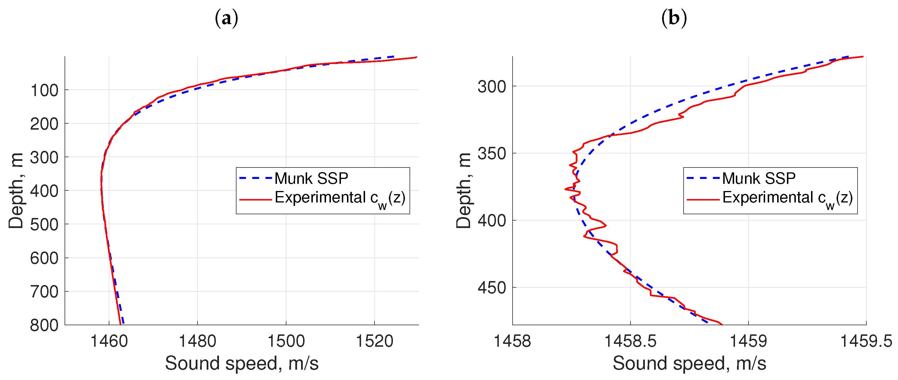
We fit the SSP, obtained by averaging the experimental profiles observed at the measurement points at the largest distances from the eddy center, by the formula from Equation (2), using the method of least squares. The averaged experimental background SSP and its approximation by the Munk formula are shown in Figure 3a,b. Note that in practical problems, only the approximation of sound speed on the interval $z\in [z_1-L/2,z_1+L/2]$ of a few hundred meters below and above the SOFAR axis is important (as refracted–refracted modes are mostly responsible for acoustic wave propagation in the channel). It is interesting to assess the sensitivity of the approximation parameters to the variations in the interval length L.

The parameters $z_1,c_1,B,ϵ$ of the Munk profile estimated using the least squares method for different spans L of measurement data points are presented in

Table 1. Optimal parameters for Munk SSP approximation for different lengths of the fitting interval L (the profile parameters are optimized for $z_1-L/2<z<z_1+L/2$).

$\mathit{L}/2$, m	$\mathit{ϵ}$	B, m	RMSE	Max. Deviation
50	$1.1\times {10}^{-3}$	186	4.43 $\times {10}^{-2}$	$0.92\times {10}^{-1}$
100	$0.9\times {10}^{-3}$	187	$5.04\times {10}^{-2}$	$1.41\times {10}^{-1}$
200	$1.0\times {10}^{-3}$	194	$8.17\times {10}^{-2}$	$3.05\times {10}^{-1}$

. Note that the parameters $z_1,c_1$ do not depend on L, since they physically correspond to the depth of the SOFAR axis and the minimum sound speed value.

Despite the fact that the Munk formula from Equation (2) provides a reasonably accurate approximation for the background SSP observed in the experiment, it is somewhat inconvenient to use within the framework of the theory of normal modes, since horizontal wave numbers and eigenfunctions of modes can only be found numerically. Recall that an acoustic field in a range-independent waveguide can be represented as a superposition of normal modes ${\varphi }_j\left(z\right)$ [1]

$$P(r,z,\omega )=\sum _j{A}_j\left(r\right){\varphi }_j\left(z\right),$$

(3)

where the expansion coefficients $A_j\left(r\right)$ are called mode amplitudes. Now, we propose another parameterization of the background SSP, for which the eigenfunctions ${\varphi }_j\left(z\right)$ can be found analytically. These eigenfunctions satisfy the following equation:

$${\varphi }_{zz}+{\displaystyle \frac{{\omega }^2}{c^2\left(z\right)}}\varphi =k^2\varphi ,$$

(4)

where k are their respective horizontal wavenumbers, and $c\left(z\right)$ is the sound speed profile. Observe that Equation (4) is formally equivalent to the one-dimensional stationary Schrödinger equation for a quantum particle in the potential $V\left(x\right)$

$${\Psi }_{xx}-V\left(x\right)\Psi =-E\Psi ,$$

(5)

where $\Psi$ is the eigenfunction of a stationary state, and E is the corresponding eigenvalue of the Hamiltonian. The quantity $-{\displaystyle \frac{{\omega }^2}{c^2\left(z\right)}}$ from Equation (4) corresponds to the quantum mechanical potential $V\left(x\right)$ from Equation (5). In this paper, we approximate $-{\displaystyle \frac{{\omega }^2}{c_0^2\left(z\right)}}$ by the so-called Morse potential [21], which is determined by the following equation:

$$-{\displaystyle \frac{{\omega }^2}{c_0^2\left(z\right)}}=c_1+D_e{(1-\exp (-a(z-z_1)))}^2,$$

(6)

where $z_1$ is the depth of the SOFAR axis, $c_1$ is the value of the potential on the SOFAR axis, and $D_e$ is the equivalent difference in the potential between the SOFAR axis $z\to \infty$.

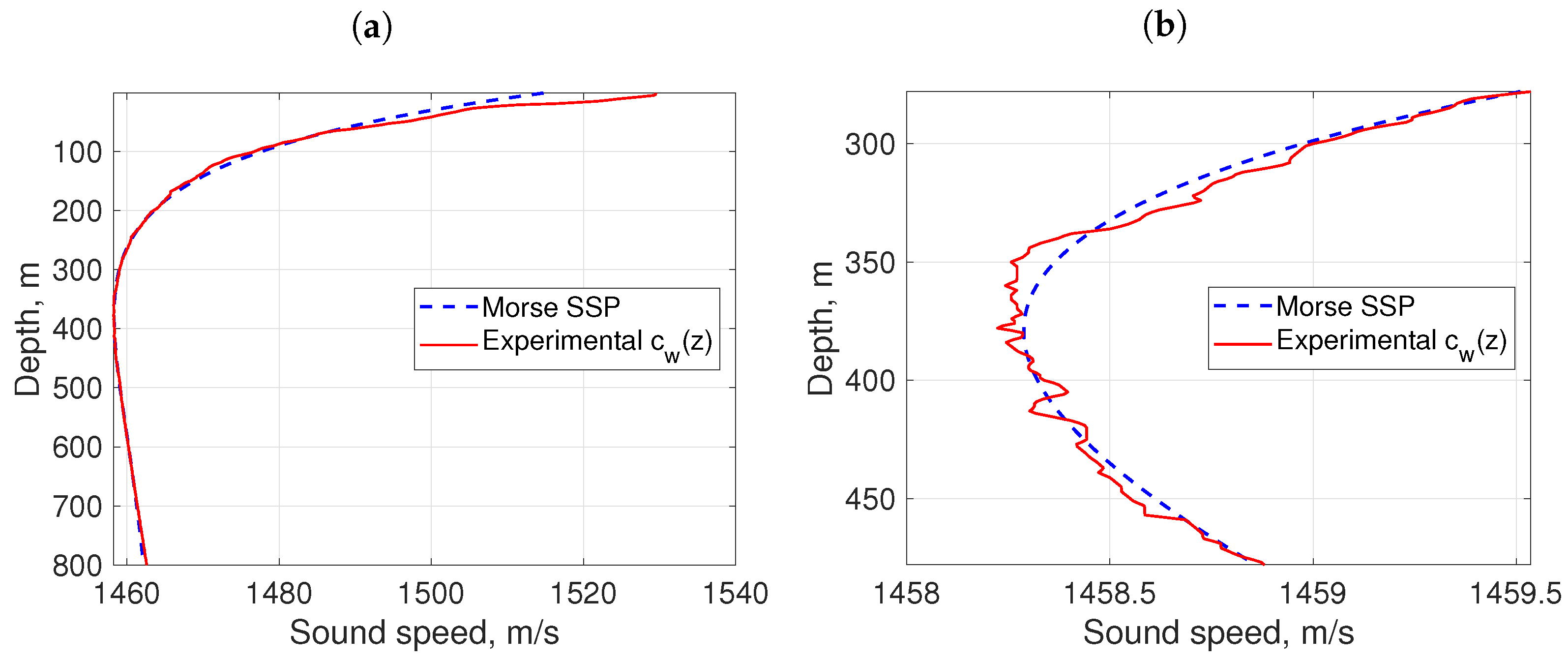
This potential seems appropriate, since within the $L/2$-neighborhood of the SOFAR axis, the graph of the sound velocity $c\left(z\right)$ determined by Equation (6) is qualitatively similar to the background SSP in the sea area around the eddy. The function ${\displaystyle \frac{{\omega }^2}{c_0^2\left(z\right)}}$ from the experimental data was fitted by the Morse formula using the least squares method for various spans of the measurement data L. The optimal parameter values $z_1,c_1,D_e$ are presented in

Table 2. Optimal parameters for Morse potential approximation for different lengths of the fitting interval L (the profile parameters are optimized for $z_1-L/2<z<z_1+L/2$).

$\mathit{L}/2$, m	${\mathit{D}}_{\mathit{e}}$	a	${\mathit{c}}_1$	RMSE	Max. Deviation
50	$2.83\times {10}^{-2}$	$3.80\times {10}^{-3}$	$-2.97$	$1.74\times {10}^{-4}$	$3.56\times {10}^{-4}$
100	$2.50\times {10}^{-2}$	$3.80\times {10}^{-3}$	$-2.97$	$2.02\times {10}^{-4}$	$3.79\times {10}^{-4}$
200	$2.58\times {10}^{-2}$	$3.60\times {10}^{-3}$	$-2.97$	$2.53\times {10}^{-4}$	$8.24\times {10}^{-4}$

, and Figure 4a,b show the agreement between the obtained parameterization and the averaged background SSP in the experimental data.

4. Analytical Calculation of Eigenfunctions and Eigenvalues in Comparison with Numerical Calculation Results

Analytical expressions for calculating eigenfunctions and eigenvalues for the Schrödinger Equation (5) with the Morse potential are given in many studies [21,22,23]. We now use these results and the simple correspondence between the variables of the Helmholtz and Schrödinger equations to express solutions to Equation (4) with the Morse potential (6)

$$\begin{array}{c}{\varphi }_j\left(z\right)=N_j{\zeta }^{{\displaystyle \frac{{\alpha }_j}{2}}}\exp (-{\displaystyle \frac{\zeta }{2}})L_j^{{\alpha }_j}\zeta ,\zeta =2\lambda \exp (-a(z-z_e)),0<\zeta <\infty ,\\ k_j^2=-c_1-D_e+{\displaystyle \frac{{\alpha }_j^2{a}^2}{4}},j=0,1,\cdots ,\lfloor \lambda \rfloor ,\end{array}$$

(7)

where $L_j^{{\alpha }_j}\left(\zeta \right)$ are Laguerre polynomials, $\lfloor \lambda \rfloor$ is the largest integer less than $\lambda$, and

$$N_j=\sqrt{{\displaystyle \frac{j!{\alpha }_{j}a}{\Gamma (j+{\alpha }_j+1)}}},{\alpha }_j=2\lambda -2j-1,\lambda ={\displaystyle \frac{\sqrt{D_e}}{a}}.$$

(8)

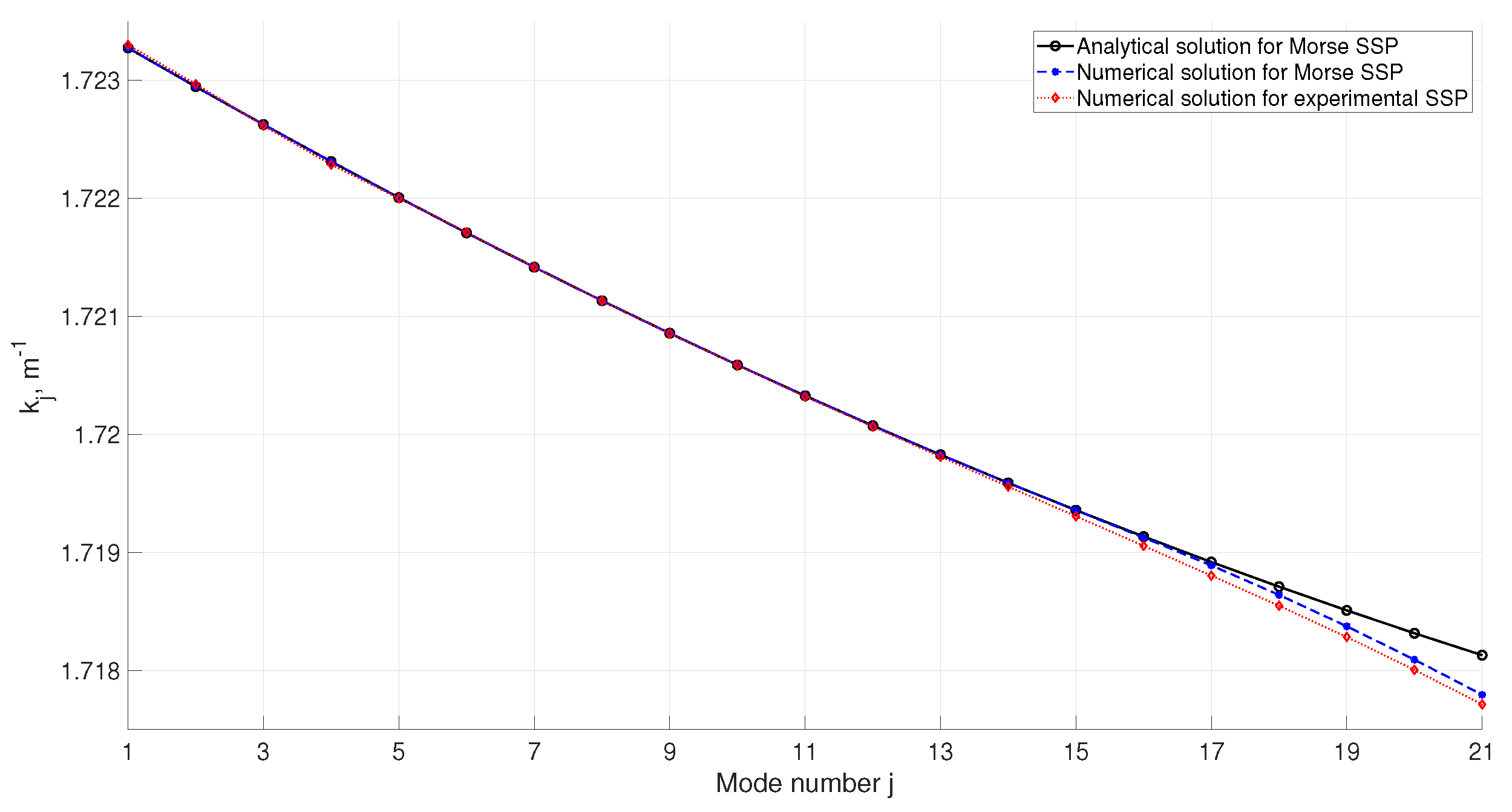
The results of computation of horizontal wavenumbers and mode eigenfunctions by Equations (7) and (8) are presented in Figure 5 and Figure 6, respectively. They are compared against the results obtained by high-accuracy numerical solution of the Sturm–Liouville problem for Equation (4) computed both for the background SSP from the experiment and for its approximation by the Morse formula (here and throughout the rest of this study we perform computations for sound frequency $f=400 \mathrm{Hz}$). Reference numerical solutions are obtained using AC_MODES software package [24] in which the computation of normal modes is implemented by the method of finite differences.

One can see excellent qualitative and quantitative agreement between the modes approximated using the Morse profile and the modes by a direct numerical solution. A noticeable difference in wavenumbers for higher-order modes can be explained by the fact that the experimental background SSP is approximated by the Morse formula only locally, i.e., within a finite interval $[z_1-L/2,z_1+L/2]$. For modes of sufficiently high-order j, the turning points of their corresponding rays lie outside this interval, and the analytical formulae proposed above do not catch the variations of their eigenfunctions far from the channel axis properly.

The comparison of eigenfunctions of modes ${\varphi }_j\left(z\right)$ computed numerically and their counterparts obtained using the analytical Formula (7) for the Morse profile is presented in Figure 6 for different mode numbers j. While for low-order modes (up to $j=10$) corresponding to paraxial propagation in the deep sound channel perfect agreement can be observed, there are slight discrepancies in higher-order modes away from the channel axis (see Figure 6d). These discrepancies would not play a significant role in the modeling of sound propagation, especially in acoustic ranging and navigation problems.

For numerical calculations of wavenumbers and modal functions, the ac_modes program was used [24], which the authors use for solving such problems [25,26]. Note that for low-order modes (i.e., for near-axial sound propagation in the SOFAR channel) which usually carry most of the energy during propagation, for example, navigation signals [26,27], the results of calculations using the Morse potential are in good agreement with the results of calculations of the ac_modes program, in which the Sturm–Liouville problem for normal modes is solved numerically using the finite difference method.

5. Parameterization of Sound Speed Perturbation Due to a Synoptic Eddy

The next step is parameterization of a perturbation of the background SSP caused by the presence of a synoptic eddy. We obtain the perturbation $\delta c(r,z)$ from the measurement data, according to Equation (1), i.e., by subtracting the background SSP $c_0\left(z\right)$ corresponding to the Morse potential from the sound speed distribution $c(r,z)$ observed in the experiment. The resulting perturbation $\delta c(r,z)$ is presented in Figure 7a and Figure 7c for the meridional and zonal transects, respectively.

As can be seen from the figures, this perturbation is localized in space. This fact confirms that our approach based on the field decomposition according to the formula from Equation (1) is adequate for the considered dataset. The authors of [28,29] proposed a parameterization of synoptic eddies (in the context of sound propagation problems) based on Gaussian functions of the following form:

$$\delta c(r,z)=c_m\exp \left(-r^2/r_r^2\right)\exp \left(-{(z-z_0)}^2/r_z^2\right),$$

(9)

where $c_m$ is the magnitude of the sound speed perturbation, $z_0$ is the depth of the eddy center, and the values $r_r,r_z$ determine the horizontal and the vertical size of the eddy, respectively.

Apparently, the formula from Equation (9) is not fully adequate for the dataset considered here, since it assumes the reflection symmetry of the eddy around the line $z=z_0$, which is not observed in our case. For this reason, we used the Maxwell–Boltzmann distribution to parameterize the sound speed field perturbation $\delta c(r,z)$ in z direction. We also take into account that this eddy may not possess a rotational symmetry with respect to a vertical line $r=0$, i.e., that sound speed isolines in a horizontal plane near the eddy are ellipsoidal rather than circular and that the intersection point of meridional and zonal transects may not exactly coincide with the center of the eddy.

We, therefore, start with the assumption that the eddy center is located at the point $(x_0,y_0)$ in the Cartesian coordinate system with the origin at the intersection point $(x=0,y=0)$ of the two transects. Hence, $\delta c(x,y,z)$ can be parameterized as follows:

$$\begin{array}{c}\delta c(x,y,z)=-c_m\exp \left[-{\displaystyle \frac{{(x-x_0)}^2}{r_x^2}}\right]\exp \left[-{\displaystyle \frac{{(y-y_0)}^2}{r_y^2}}\right]\\ \times \left({\displaystyle \frac{z-z_0}{r_z}}\right)\exp \left[-{\displaystyle \frac{\beta {(z-z_0)}^2}{r_z^2}}\right],\end{array}$$

(10)

where $\beta$ is the Maxwell–Boltzmann distribution parameter related with the asymmetry of the distribution along the z axis, and $r_x,r_y$ determine the characteristic size of the eddy in the directions along the meridian and the parallel, respectively.

The optimization of the values of $\beta ,r_x,r_y,r_z,y_0,x_0,z_0,c_m$ for this parameterization simultaneously over the two transects of the sound speed field $\delta c(r,z)$ was performed using the least squares method. As in the previous section, the optimization was performed using the data from the depth interval limited by $L=200 \mathrm{m}$ about the deep sound channel axis. The optimal values are presented in

Table 3. Optimal parameters for approximation of sound speed field perturbation by Formula (10).

$\mathit{\beta }$	${\mathit{r}}_{\mathit{x}}$, km	${\mathit{r}}_{\mathit{y}}$, km	${\mathit{r}}_{\mathit{z}}$, m	${\mathit{x}}_0$, km	${\mathit{y}}_0$, km	${\mathit{z}}_0$, m	${\mathit{c}}_{\mathit{m}}$, m/s
1.7125	32	18	250	6	4	67.5	3.5

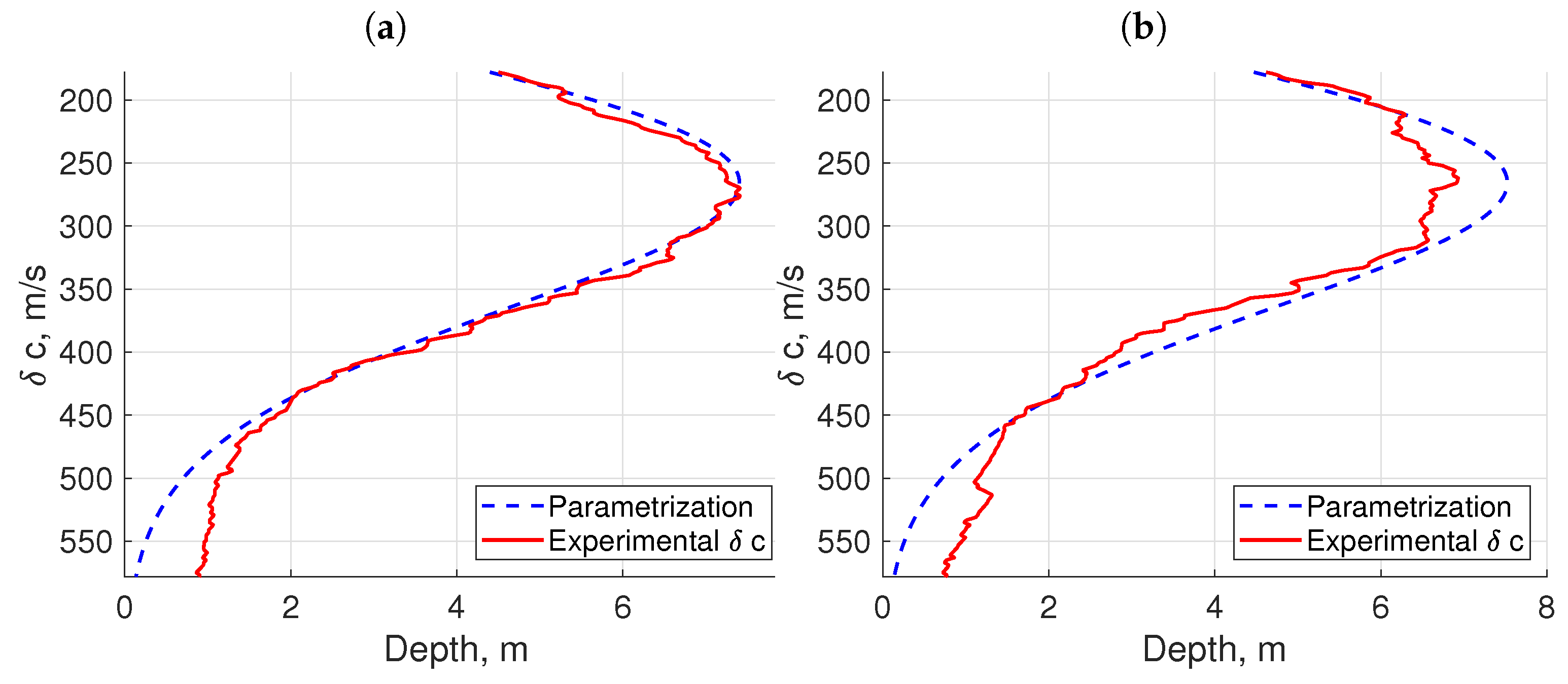
, and the resulting perturbations of sound speed fields for meridional ($\delta c(0,y,z)$) and zonal ($\delta c(x,0,z)$) transects are depicted in Figure 7b and Figure 7d, respectively. In addition, experimental and parameterized perturbations of the SSPs ($\delta c(0,0,z)$) at the eddy center for the zonal and meridional transects are presented in Figure 8a and Figure 8b, respectively.

The standard deviation for the optimal parameterization is $0.38 \mathrm{m}/\mathrm{s}$, and the maximal one is $2.05 \mathrm{m}/\mathrm{s}$. Despite the fact that the latter value is not very small, it is clearly associated with the data outliers at the periphery of the eddy. As can be seen from Figure 7, this deviation is much smaller in the eddy center area; hence, it can be concluded that Equation (10) adequately reproduces the sound speed field perturbation $\delta c(x,y,z)$.

6. Calculation of Eigenfunctions and Eigenvalues in the Presence of an Eddy

As is mentioned in the previous sections, the wavenumbers for the background SSP calculated using analytical formulae for the Morse potential are in good agreement with the numerical results for the real background SSP observed in the experiment. In order to achieve an analytical description (modulo some quadratures) of the sound propagation through an eddy, we can use the perturbation theory for normal modes [1] in the underwater sound channel to evaluate horizontal wavenumbers in the neighborhood of the center of the eddy.

We start with the standard equations of perturbation theory [1,21] (up to the second order), written as follows:

$$\begin{array}{cc}\hfill & K^2(x,y,z)=K_0^2\left(z\right)+\nu (x,y,z),\hfill \\ \hfill & k_j^2(x,y)=k_{j,0}^2+\delta k_j^2(x,y)+{\delta }^2{k}_j^2(x,y)\cdots ,\hfill \\ \hfill & \delta k_j^2(x,y)={\int }_0^H{\displaystyle \frac{\nu (x,y,z){\varphi }_j^2\left(z\right)}{\rho \left(z\right)}}dz,\hfill \\ \hfill & {\delta }^2{k}_j^2(x,y)=\sum _{l\ne j}{\displaystyle \frac{1}{k_{j,0}^2-k_{l,0}^2}}{\int }_0^H{\displaystyle \frac{\nu (x,y,z){\varphi }_j\left(z\right){\varphi }_l\left(z\right)}{\rho \left(z\right)}}dz,\hfill \end{array}$$

(11)

where $K_0\left(z\right)={\displaystyle \frac{\omega }{c_0\left(z\right)}}$ is the medium wavenumber for the background SSP, $K(x,y,z)$ is the eddy-perturbed medium wavenumber, and $\nu (x,y,z)$ is the difference in their squares (this value corresponds to the potential perturbation in quantum mechanics). By $k_{j,0}$, we denote the horizontal wavenumbers of modes calculated for the background SSP, ${\varphi }_j\left(z\right)$ are their corresponding eigenfunctions, and $\delta k_j^2(x,y)$ and ${\delta }^2{k}_j^2(x,y)$ are the perturbations of horizontal wavenumbers squared due to the presence of the eddy. The mode perturbation theory [1,21] may also be used to calculate eigenfunctions for an eddy-perturbed SSP, which may be presented in the form of a series over unperturbed eigenfunctions ${\varphi }_j\left(z\right)$ (the respective formulae can be found in any textbook on quantum mechanics, e.g., [21]).

The results of the numerical solution of the Sturm–Liouville problem for Equation (4) for the SSP $c_0+\delta c(0,0,z)$ at the eddy center (where the perturbation has the largest magnitude) are compared with the perturbation theory as elucidated in Equation (11) in Figure 9.

In this case, the blue line corresponds to the horizontal wavenumbers for the unperturbed SSP $c_0\left(z\right)$, while the red line corresponds to the SSP at the center of the eddy. Subplot Figure 9b presents the same quantities but for the half-magnitude perturbation $0.5\delta c$. The approximations according to the first- and second-order perturbation theory are shown in Figure 9 by the yellow and purple lines, respectively. In addition, the green dotted line presents the approximation by the Padé perturbation theory [30].

An acceptable accuracy of the approximation is achieved for the full-magnitude perturbation $\delta c$ only when using second-order formulae. Note, however, that this situation is somewhat extreme from the viewpoint of the perturbation theory applicability conditions. Indeed, the magnitude of the eddy-related potential perturbation exceeds half of the depth of the equivalent potential well (in terms of an equivalent quantum-mechanical problem). Physically, this results from the fact that the center of the eddy is located almost exactly at the deep sound channel axis.

As shown in Figure 9b, at the points of the eddy with the half-amplitude perturbation ${\displaystyle \frac{\delta c(x,y,z)}{2}}$, even the first-order perturbation theory gives an almost exact result (except the first few modes), while the second-order formulae for the Taylor and Padé series accurately reproduce the wavenumbers of the eddy-perturbed SSP. Note that both first-order and second-order perturbation theory offer almost the same level of convenience when using finite formulae for the numerical and analytical description of sound propagation in the ocean. Indeed, the quadratures in the last two formulae (11), that have the same structure in depth, still do not allow us to obtain an explicit expression by taking the integral. As a result, the wavenumbers $k_j^2(x,y)$ in any case will simply have the same form of dependence on $x,y$, as the speed of sound $c\left(z\right)$ in Equation (10).

7. Conclusions and Discussion

This paper presents a parameterization method for the sound speed field perturbation caused by a synoptic eddy in deep ocean. The existing parameterizations [28,29] serve as the basis for the derivation of an improved version of the equation that could better describe such a perturbation. The proposed parameterization is applied to approximate real oceanographic data collected along two perpendicular transects of a large and stable synoptic eddy during the field work in the Sea of Japan. An approximation of the background SSP by an analytical expression corresponding to the Morse potential in quantum mechanics allowed us to obtain explicit expressions for refracted-refracted acoustic modes [1] of the SOFAR channel (i.e., the modes corresponding to Brillouin rays having two turning points in the water column and not reaching the surface and the bottom). The use of these formulae and the perturbation theory for acoustic modes allowed us to obtain a convenient semi-analytical representation of the dependence of the modal wavenumbers on horizontal coordinates. The respective formulae can be used for solving two- and three-dimensional problems of sound propagation through a synoptic eddy.

As shown in Figure 10, the graphs representing the dependence of horizontal wavenumbers for low-order modes (trapped in the SOFAR channel) on range do not intersect. For sound frequencies of a few hundred Hertz, this fact indicates the adiabatic sound propagation through an eddy. In addition, this fact allows one to substantially simplify the computation of acoustic fields in the framework of normal modes theory, e.g., using mode parabolic equations [31] or the vertical modes/horizontal rays approximation.

In future work, we could use analytical parameterizations of the sound speed profile in the Sea of Japan and the perturbation due to the presence of an eddy for performing analytical simulations of acoustic waves propagation in the considered area. By contrast to a direct numerical solution of the wave equation (or the Helmholtz equation), analytical formulae for horizontal rays and mode amplitudes could provide additional insights into the physics of sound scattering by large-scale objects like synoptic eddies. An example on how this can be accomplished using separation of variables technique is [32].