Influence of Free Surface on the Hydrodynamic and Acoustic Characteristics of a Highly Skewed Propeller

Abstract

The noise analysis of a large-scale aquaculture vessel reveals that during its navigation, the primary equipment noise, particularly from the propeller, exerts a notable influence on the aquaculture environment for large yellow croaker. The free surface greatly impacts the noise performance of propellers, which is a significant factor affecting the fish’s habitat. This study adopts the numerical simulation method to analyze the hydrodynamic and acoustic characteristics of the E1619 propeller operating near the free surface. The open-water performance and noise calculations of the propeller are verified through experiments, and the effects of different immersion depths and advance coefficients on the propeller are explored. The results demonstrate that the free surface significantly affects the thrust, torque, and noise of the propeller, especially at shallow immersion depths and low advance coefficients. Surface wave pattern causes the instability and breakup of tip vortices, causing increased thrust and torque fluctuations, reduced efficiency, and significant overall sound pressure levels in the entire flow field. As immersion depth and advance coefficients increase, the interaction between tip vortices and the free surface weakens, wake vortex instability decreases, and noise levels gradually reduce. These analyses and conclusions can guide the design of next-generation propellers for aquaculture vessels to optimize performance near the free surface.

1. Introduction

When ships such as aquaculture vessels navigate under ballast conditions or submarines operate on the surface, the propeller blades are positioned close to the free surface. Under such conditions, the free surface can significantly affect the propeller flow, potentially leading to ventilation, degraded propulsion performance, and vibration [1]. The free surface notably impacts the hydrodynamic performance of the propeller beneath it, while the propeller’s wake, in turn, influences the shape of the free surface. Di Mascio et al. [2] elucidated part of the mechanism under low-load conditions without considering the air phase. Moreover, the impact of the free surface on propeller noise is also significant. Complex flow phenomena near the free surface, such as wave generation and breaking, disrupt the flow around the propeller blades. Disturbances from the free surface create non-uniform inflow conditions, causing uneven forces on the propeller blades, which induce unsteady flow-generated noise. This noise is not only related to the propeller’s load but is also modulated by the frequency of free surface oscillations. While research exists on the hydrodynamics and wake characteristics of propellers beneath free surfaces, the intricate interaction mechanisms between the free surface and propeller noise remain inadequately understood. Researching noise for aquaculture vessel propellers operating near free surface is crucial to address issues such as fish being startled, stopping feeding, or even dying due to excessive environmental noise of aquaculture water. Effective noise control will create a favorable living environment within the aquaculture tanks, ensuring successful fish farming.

In recent years, many researchers including Orihara and Miyata [3], Arribas [4], and Sadat-Hosseini et al. [5] have adopted numerical methods to investigate the motion of ships under adverse sea conditions. Hence, investigating the impact of the free surface on the flow field and noise characteristics of propellers is vital to ensuring the safe operation of ships in complex motion and wave environments. Variations in the immersion depth and advance coefficient of the propeller create significant risks due to interactions between the vessel and the free surface. These interactions not only introduce additional resistance but also increase the load on the blade surfaces of the propeller, which was also observed by Chuang and Steen [6] and Ueno et al. [7]. Moreover, the strong interference of the free surface with vortex structures can reduce propulsion efficiency of the propeller and increase radiated noise due to wake flow instability. Therefore, studying the hydrodynamic and noise characteristics of interactions between the propeller and free surface under different operating conditions is of great significance. Yu et al. [8] investigated the evolution and flow dynamics within the wake of a propeller, providing important insights for improving the design and optimization of marine propellers. A deeper understanding of flow under complex environment can assist researchers in designing more efficient propellers for aquaculture vessels, as concluded by Sun et al. [9] and Zhou et al. [10].

Research on the open-water performance of propellers has achieved substantial results by Gong et al. [11], Chase [12], Wang et al. [13], and Baek et al. [14], but there are still deficiencies in the study of propeller characteristics near the free surface. Kozlowska et al. [15,16] conducted extensive research on the load variation mechanism of a propeller under suction conditions, suggesting that the vortex structures attached to the suction side of the blades were crucial for load variation. Kwang-Jun Paik [17] performed numerical simulations of model propellers at various advance coefficients and immersion depths, finding that interactions of the propeller with the free surface caused fluctuations in thrust and torque, distortions in the tip vortex trajectories, and an increased rate of decrease in thrust and torque with higher advance coefficients. Califano and Steen [18] confirmed that the tip vortex of conventional propellers was an important factor forming suction conditions. Paik et al. [19] provided velocity distributions and surface wave patterns upstream and downstream of a propeller near the free surface. Wang et al. [20] conducted both numerical and experimental investigations to analyze the hydrodynamic performance of the submarine at three different immersion depths and advance coefficients, showing that interactions between the hull and free surface significantly affected the inflow conditions, flow field characteristics, and the load on the propeller blades. Shallow immersion depths led to strong free surface fluctuations, which caused instability of the flow field. Lungu [21] adopted a numerical method to predict the hydrodynamic performance of a self-propulsion submarine near the free surface and compared results of three immersion depths to highlight the impact of free surface on propulsion performance. The study also found that the detached eddy simulation (DES) method provided higher accuracy than the unsteady Reynolds-averaged Navier–Stokes (URANS) method, and achieved comparable results to the more computationally demanding large eddy simulation (LES) method.

The underwater radiated noise of ships primarily comprises mechanical noise, hydrodynamic noise, and propeller noise [22]. At low speeds, when the propeller does not cavitate, mechanical noise has the greatest impact, with propeller noise being the second most significant source. However, the noise levels of these two sources are quite close. Moreover, in recent decades, advancements and applications in active and passive control technologies have significantly reduced mechanical noise, making propeller noise increasingly prominent. Propeller noise not only dominates in noise levels but also exhibits unique acoustic characteristics [23]. Underwater propeller noise is particularly important as it can be detected by sonar from hundreds of meters away [24].

Investigations on noise characteristics of the propeller beneath the free surface are relatively scarce, with most studies focusing on noise performance under infinite immersion depths. Sezen and Atlar [25] utilized a hybrid method combining DES with the Ffowcs-Williams and Hawkings (FW-H) method and penetration formula for numerical calculations. The results indicated that, using the permeable surface method around the entire submarine revealed more pronounced spectral peaks caused by tip vortex flow than those of the permeable surface around the propeller. The interaction between cavitation around the hull and nonlinear noise sources affected the amplitude of characteristic peaks. Özden et al. [26] numerically investigated the flow field and noise performances around the propeller using the URANS method combined with the FW-H model for underwater acoustic analysis, comparing noise characteristics in self-propulsion and imposed wake conditions. The study found that the spectral curves for both conditions showed similar amplitudes with slight differences, and the noise level comparisons showed reasonable correlations. This suggested that imposed wake flows could be adopted to estimate sound pressure levels of the propeller when hull geometries were not available but wake characteristics were present. Chen et al. [27] conducted numerical investigations into the impact of varying geometric inflows on the hydrodynamic and acoustic performance of propellers. Their study established a correlation between water pressure and propeller thrust, enabling the estimation of propeller thrust at different immersion depths.

Propeller noise includes cavitating and non-cavitating types. This study examines how propeller rotation generates noise, especially during cavitation, when bubbles form and collapse around blades. Measures like larger propeller diameters, lower speeds, high skew angles, and improved wake uniformity can significantly reduce cavitation noise. Using the high-skew E1619 propeller helps distribute blade load, reduce pressure fluctuations, and control cavitation sites, effectively lowering noise. With cavitation minimized, non-cavitating noise becomes more relevant [28], including broadband and tonal noise from turbulent interactions and wake effects [29]. This study focuses on non-cavitating noise using simulations, excluding hull vibration and cavitating noise.

Due to the limited research on the interference of large skewed propellers with free surface at different depths and loading conditions, especially regarding noise characteristics, this study adopts the improved delayed detached eddy simulation (IDDES) method combined with the SST k-ω turbulence model to simulate the hydrodynamic and noise characteristics of a propeller near the free surface under different immersion depths and advance coefficients. By performing numerical simulations on the propeller at four immersion depths and four advance coefficients, the study investigates the impact of the free surface on thrust, torque, efficiency, and noise characteristics. The results reveal that the free surface significantly affects the hydrodynamic performance of the propeller, especially at shallow immersion depths and low advance coefficients. Surface wave fluctuations lead to wake vortex instability, changes in blade surface pressure, and fluctuations in turbulent kinetic energy, resulting in greater fluctuations in thrust and torque, reduced efficiency, and higher noise levels in the far field. Additionally, disturbances from the free surface create non-uniform inflow conditions, causing uneven forces on the propeller blades and increasing unsteady flow-induced noise. To reduce cavitation noise, the study selects a high-skew propeller and focuses on non-cavitating noise, demonstrating that high-skew propellers effectively reduce cavitation noise generation. Finally, the FW-H acoustic model is used to analyze the spatial distribution of noise, and the results show that the impact of the free surface on hydrodynamic performance is also reflected in the variation in noise characteristics.

2. Mathematical and Numerical Model

2.1. Numerical Methods and Flow Solver

With the continuous development and improvement of numerical computing methods and high-performance computing hardware in recent years, it has become possible to adopt complex numerical analysis methods to study the dynamics of propeller wakes. The flow is simulated utilizing the computational fluid dynamics (CFD) software STAR-CCM+ 17.04, which solves the three-dimensional incompressible Navier–Stokes (N-S) equations. The CFD analysis involves solving the control equations, which consist of the continuity equation and momentum equation, using unstructured grids based on the finite volume method (FVM) for discretization. The equations governing the motion of incompressible Newtonian fluids are known as the N-S equations [30,31]. In a Cartesian coordinate system, they can be formulated as follows:

$${\displaystyle \frac{\partial u_i}{\partial t}}+{\displaystyle \frac{\partial u_i{u}_j}{\partial x_j}}=-{\displaystyle \frac{1}{\rho }}{\displaystyle \frac{\partial p}{\partial x_i}}+\nu {\displaystyle \frac{{\partial }^2{u}_i}{\partial x_j\partial x_j}}+f_i,$$

(1)

$${\displaystyle \frac{\partial u_i}{\partial x_i}}=0.$$

(2)

where u_i and u_j are the velocity components in the x_i and x_j directions, t is the time, ρ is the density of the fluid, p is the pressure, ν represents the dynamic viscosity of the fluid, and f_i represents the force per unit mass.

The DES method integrates the characteristics of RANS in the near-wall region and LES in the far field. It was initially proposed by Spalart et al. in 1997 and was also known as DES97 [32]. The model achieves the switch between LES and RANS by modifying the dissipation term scale in RANS equations. In this study, the IDDES method using Menter’s SST k-ω model is applied. Turbulence is simulated using a combination of k-ω and k-ε models [33] in this method, where the turbulent kinetic energy k and specific dissipation rate ω are determined using the following equations (written in tensor notation) [34]:

$${\displaystyle \frac{\partial k}{\partial t}}+\left(u-{\sigma }_k\nabla v_t\right)\cdot \nabla k-{\displaystyle \frac{1}{P_k}}{\nabla }^{2}k+s_k=0,$$

(3)

$${\displaystyle \frac{\partial \omega }{\partial t}}+\left(u-{\sigma }_{\omega }\nabla v_t\right)\cdot \nabla \omega -{\displaystyle \frac{1}{P_{\omega }}}{\nabla }^2\omega +s_{\omega }=0,$$

(4)

In the equations, $s_k$ and $s_{\omega }$ are the source terms for k and ω, respectively.

The solution is obtained by employing second-order discretization in both time and space. The semi-implicit method for the pressure-linked equations algorithm is adopted to implement pressure–velocity coupling. Menter’s SST k-ω model is used for turbulence modeling. The volume of fluid multiphase model, utilizing the high-resolution interface-capturing scheme developed by Muzaferija et al., is employed to simulate the free surface and capture wave patterns produced by the propeller during operation.

The IDDES method has several advantages in turbulence simulation. Its adaptive nature allows for the use of RANS in the boundary layer and LES in separation and vortex regions, thus capturing complex separated flows and large-scale turbulent structures at a lower computational cost. Zhang et al. [35] revealed that IDDES simulations demonstrated commendable predictive capabilities in flow asymmetry, and Guo et al. [36] found that it showed significant improvement over RANS methods in capturing local flow field details. The main drawbacks of the IDDES method include its high dependence on mesh resolution and model parameters, especially in the transition between RANS and LES regions, where errors can arise, leading to distortion of turbulent structures. Posa et al. [37] and He et al. [38] found that IDDES is unsuitable for near-wall flow instabilities involving wake dynamics, Reynolds stresses, turbulent kinetic energy, and pressure fluctuations.

2.2. FW-H Method

In this study, noise analysis is conducted using acoustic analogy theory [39], which assumes that acoustic signals from the flow propagate through a stationary, uniform, and unbounded medium without influencing the flow. The FW-H equation, utilizing the most comprehensive form of Lighthill’s acoustic analogy, can predict sound generated by equivalent sources such as monopoles, dipoles, and quadrupoles. To directly calculate the time variation in sound pressure or acoustic signals at specific receiver locations, the time-domain integral formula evaluates a limited surface area integral. This requires precise time resolution of flow field variables on the source (emitting) surface to accurately evaluate the surface integrals. The FW-H equation extends Lighthill’s acoustic analogy model to include arbitrary motion of general surfaces, making it the most versatile form. In the equation, the surface where f(x,t) = 0 is mathematically represented to define the noise source data, where x denotes the Cartesian spatial coordinates of the undisturbed medium and t denotes time. Assuming f > 0 indicates the exterior of the control surface and f < 0 indicates the interior, the FW-H equation is then formulated as follows:

$$\begin{array}{l}{\displaystyle \frac{1}{a_0^2}}·{\displaystyle \frac{{\partial }^2{p}^{\prime }\left(x,t\right)}{\partial t^2}}-{\nabla }^2{p}^{\prime }\left(x,t\right)={\displaystyle \frac{\partial }{\partial t}}\left\{\left[{\rho }_0{v}_n+\rho \left(u_n-v_n\right)\right]\delta \left(f\right)\right\}-\\ {\displaystyle \frac{\partial }{\partial x_i}}\left\{\left[P_{ij}{n}_j+\rho u_i\left(u_n-v_n\right)\right]\delta \left(f\right)\right\}+{\displaystyle \frac{{\partial }^2}{\partial x_i\partial x_j}}\left\{T_{ij}H\left(f\right)\right\}\end{array},$$

(5)

In the equation, a₀ represents the far-field speed of sound, p′(x,t) represents the sound pressure at the observation point, u_i represents the fluid velocity component in the x_i direction, u_n is the fluid velocity normal to the surface where f = 0, and v_n is the surface velocity normal to the surface. $\delta \left(f\right)$ is the Dirac-δ function, H(f) represents the Heaviside function, ρ₀ and ρ represent the densities of the static medium and the fluid, respectively, T_ij represents the Lighthill equivalent stress tensor, and P_ij represents the compressive stress tensor.

The FW-H acoustic model performs well in low-frequency noise prediction and flow noise simulation for complex geometries, effectively combining flow and acoustic predictions. This model has been used to study far-field noise of pitching airfoils in inviscid flow [40] and far-field noise from jet-flap interactions in turbulent flow [41]. However, calculating the quadrupole term requires a volume integral over regions surrounding the fuselage and control surfaces, which incurs high computational costs. Furthermore, the difficulty in selecting an appropriate integration region can lead to uncertainties in accuracy and randomness of the results [42,43].

This study conducts a three-dimensional numerical simulation of a propeller operating in open water, focusing on incompressible, separated, and unsteady flow conditions. The momentum and continuity equations are resolved utilizing a grid-centered FVM with a decoupled solution strategy, and the IDDES method is adopted to evaluate the unsteady hydrodynamic performance of a highly skewed propeller [44]. Upon achieving convergence in the force and flow field distributions, the FW-H acoustic model is employed to determine the far-field radiated noise from the propeller [45]. This technique, which addresses the acoustic field once the flow field is stabilized, improves computational efficiency and speeds up the convergence of the acoustic field results.

3. Geometry and Simulation Conditions

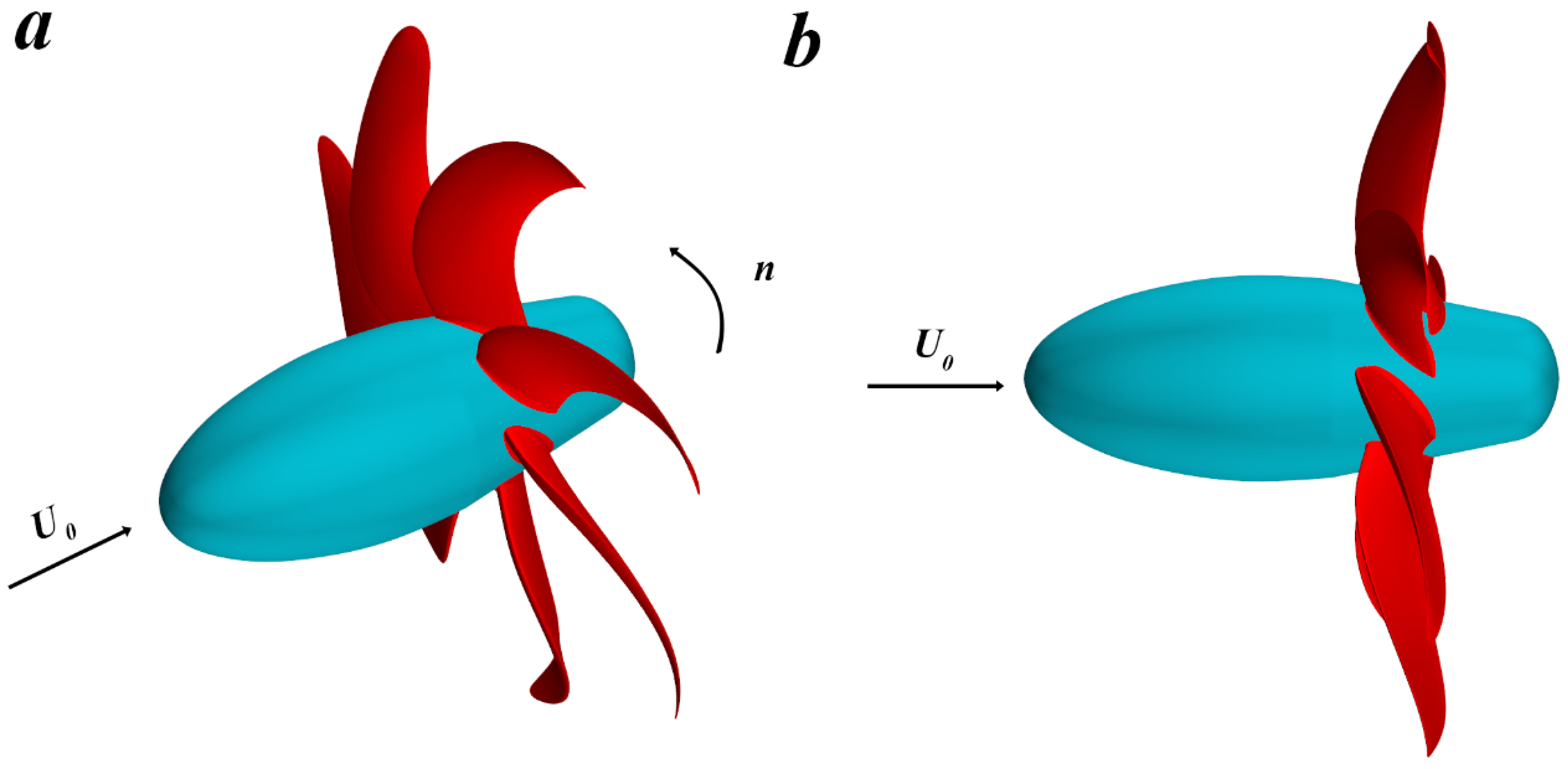
3.1. Geometric Model

The E1619 propeller is a 7-blade large skew propeller proposed and designed by CNR-INSEAN (Institute of Marine Engineering-National Research Council, Rome, Italy). Detailed information can be found in the literature. The three-dimensional representation of the E1619 propeller is shown in Figure 1. In 2009, Di Felice et al. [46] completed open-water hydrodynamic model tests of E1619 propeller in the INSEAN towing tank. However, the specific test conditions, scale ratio, and rotational speed are not available. In this study, the diameter and rotational speed of the model propeller used are the same as those in the work by Chase and Carrica [47] on the hydrodynamic performance of E1619 propeller behind the ship.

The key parameters of the propeller are listed in

Table 1. E1619 propeller’s main parameters.

Quantity	Symbol	Unit	Value
Number of blades	B	-	7
Propeller diameter	D	mm	485
Propeller radius	R	mm	242.5
Propeller/Hub diameter ratio	Dhub/D	-	0.226
Pitch at r = 0.7R	P0.7R	-	1.15
Chord at r = 0.75R	c0.75R	mm	6.8

, where B represents the number of propeller blades, D is the propeller diameter, R is the propeller radius, D_hub is the hub diameter, P_0.7R is the pitch ratio at 0.7 times the propeller radius, and c_0.75R is the chord length of the blade section at 0.75 times the propeller radius.

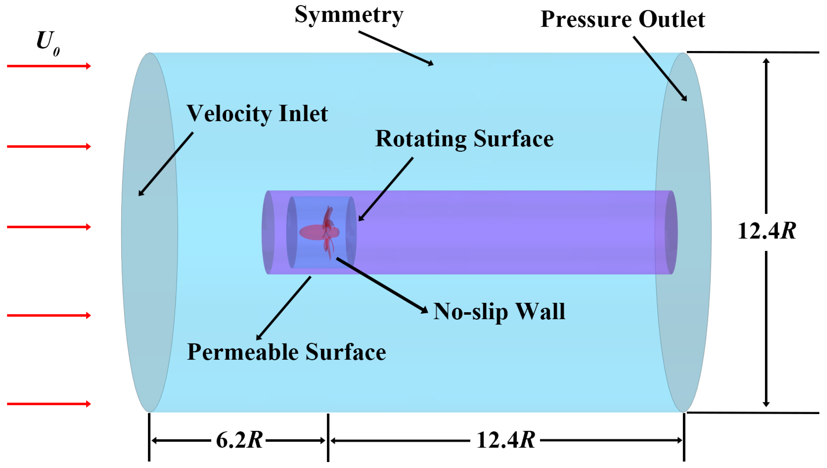
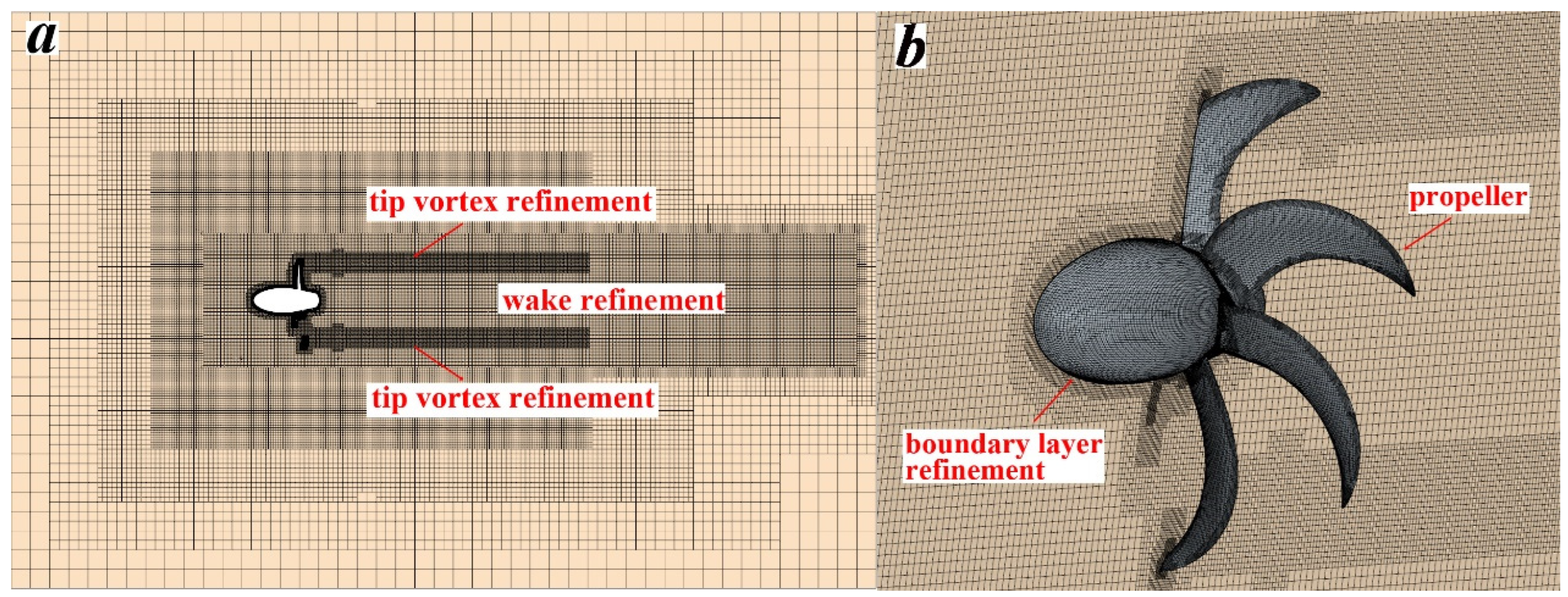
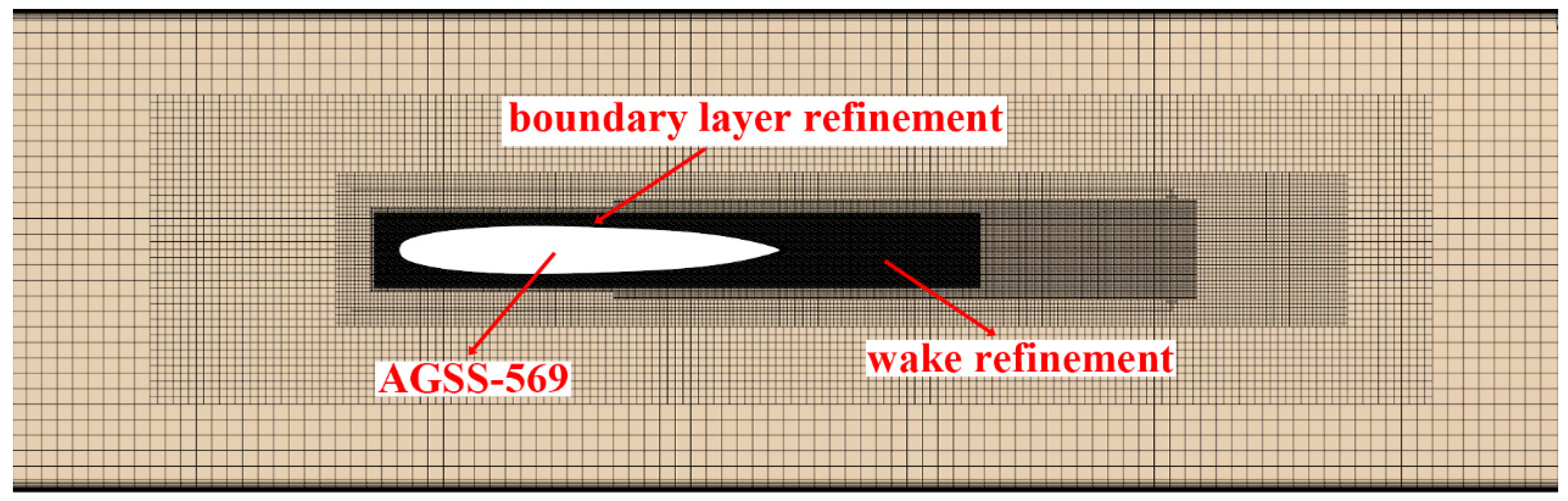
3.2. Boundary Conditions and Mesh Details

This study defines two types of computational domains: infinite depth and finite depth. The dimensions and boundary conditions for the infinite depth domain are depicted in Figure 2, with the coordinate system’s origin located at the propeller’s center. For the finite depth domain, wave damping was applied to all boundaries, with a damping wavelength of 6R. The setup and mesh generation for the computational domain were based on the geometric model, aligning the entire propeller within a cylindrical flow field centered on the hub’s axis. The computational domain was divided into three regions: the background domain, the penetration domain, and the rotating domain. In the background domain, the inflow boundary was set with a velocity inlet condition, and the outflow boundary has a pressure outlet condition. Other boundaries were set as symmetry planes. The surfaces of the penetration domain, rotating domain, and propeller were all set as no-slip walls. A sliding mesh method was employed to simulate the propeller’s rotation. The cylindrical fluid computation domain had a diameter of 12.4R, with the distance from the propeller center to the inlet being 6.2R and the distance to the outlet being 12.4R. The penetration domain, a cylinder with a diameter of 1.5R and a length of 14R, was designed to adequately capture fluctuations on the propeller surface and the radiated noise from wake vortex structures. The rotating domain, centered on the propeller, had a diameter and length of 2.5R. Boundary interfaces between the background and penetration domains, as well as between the penetration and rotating domains, facilitated information exchange and iteration between subdomains.

The computational domain was discretized using an unstructured trimmed mesher, with grid refinement applied to the propeller wake and vortex structure regions to capture the complex spatial flow. The grids were also refined on the propeller blade surfaces, feature lines, and rotating domain surface. The boundary layer on the propeller surface was discretized using prism layer mesher, with 25 boundary layers and a growth rate of 1.2. The thickness of the first boundary layer was determined based on y⁺ < 1 and the formula provided by Rodriguez [48]. Multiple cylindrical grid refinement regions were set around the propeller to adequately capture the tip vortices produced by the propeller blades and the hub vortices generated by the propeller hub. The grid distribution is depicted in Figure 3, with a total of 7.50 million cells. The time step was determined based on the time required for the propeller to complete 1° of rotation, which was 1.2 × 10⁻⁴ s. This study used the penetration surface method for integration. Ideally, the entire computational region should be considered as a penetrable integration surface, but this would result in a large computational load. Instead, the penetration domain was used for the integration. Based on the hydrodynamic results, the time step was set to the time required for the propeller to complete 0.5° of rotation, which was 6 × 10⁻⁵ s, with the acoustic model added for the calculation of radiated noise.

3.3. Numerical Validation

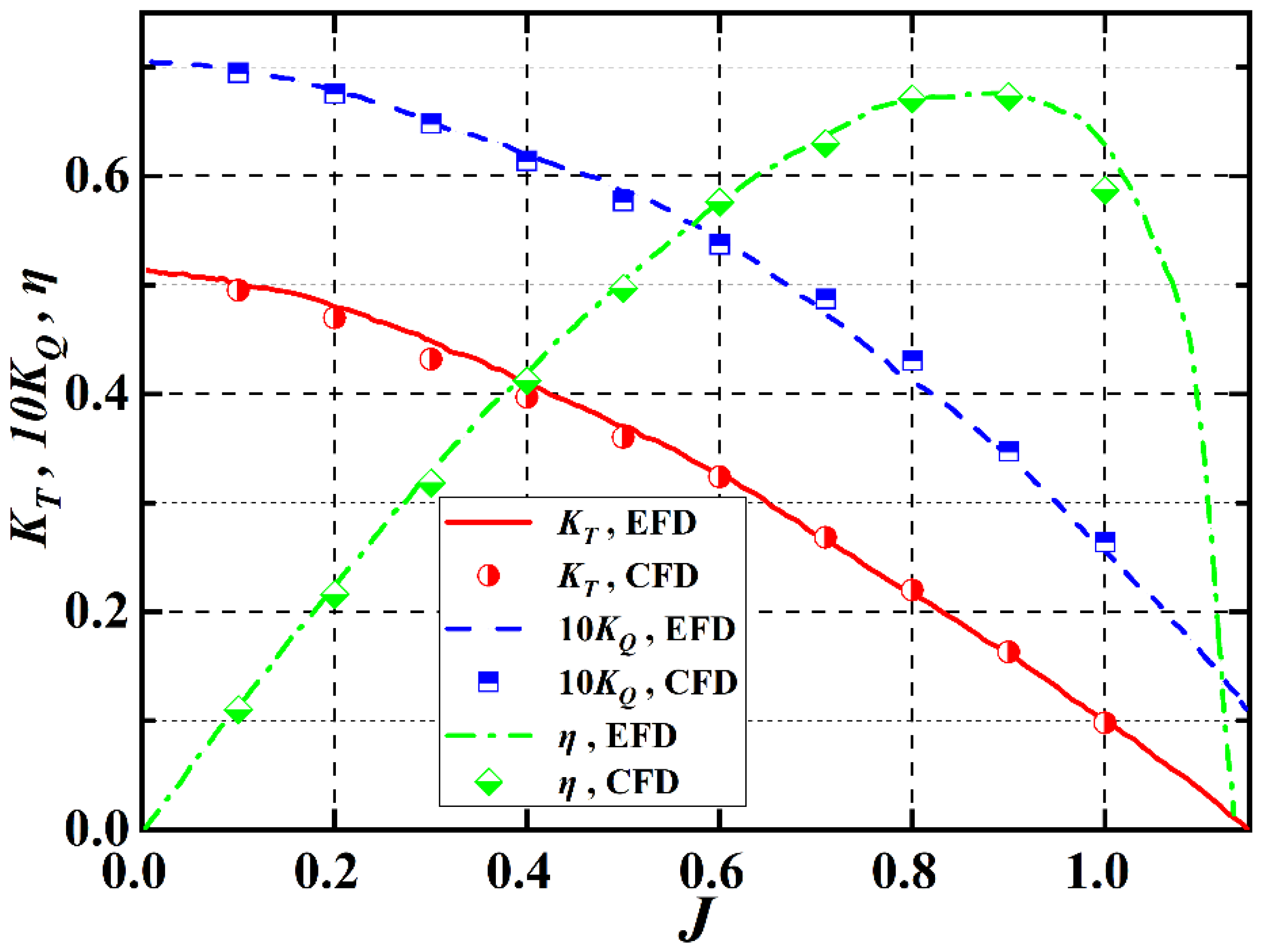
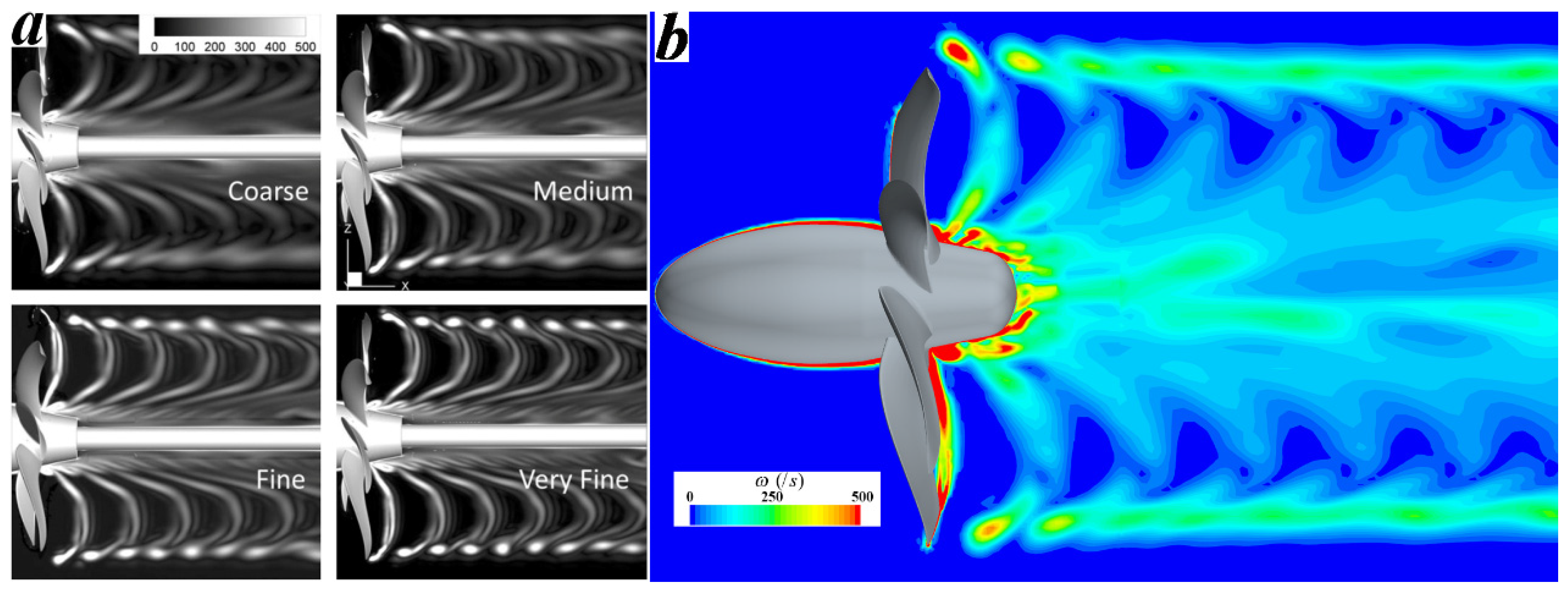
3.3.1. Hydrodynamic Performance Validation

The accuracy of the numerical method used was assessed through a grid convergence analysis involving three distinct grid sizes. To ensure correctness, numerical results were compared with experimental data. For grid convergence verification, the base grid size in the computational domain was refined while keeping the same mesh topology and keeping y⁺ between the initial mesh points and boundary layer surfaces consistent. This refinement process resulted in three grid configurations: a coarse grid with 4.34 million cells, a medium grid with 7.5 million cells, and a fine grid with 12.96 million cells. In line with the methodology suggested by Baek et al. [14] for unstructured grids, the refinement ratio $r_G$ was initially established before confirming grid independence, as this ratio is a critical parameter. The refinement ratio is defined as follows:

$$r_G={\left({\displaystyle \frac{N_{fine}}{N_{coarse}}}\right)}^{1/d},$$

(6)

In the formula, N represents the total number of grids, and d is the dimension of the computational problem.

In this study, which involves three-dimensional problems, d is set to 3. The refinement ratios for the three sets of grids are approximately 1.2, and the time step is chosen as 1.2 × 10⁻⁴ s. The simulation results for the E1619 propeller are compared with open-water experimental data, as detailed in

Table 2. The simulation results of the propeller hydrodynamic performance compared with the experimental data at J = 0.71.

J = 0.71		KT	10KQ	η
Experiment [46]		0.2657	0.4719	0.6389
Simulation	coarse grid	0.2703	0.4947	0.6175
	medium grid	0.2682	0.4873	0.6219
	fine grid	0.2676	0.4856	0.6227
Error (%)	coarse grid	1.74	4.82	3.35
	medium grid	0.95	3.27	2.66
	fine grid	0.72	2.90	2.53

. K_T, K_Q, and η are the thrust coefficient, torque coefficient, and efficiency of the propeller, respectively, defined as follows:

$$K_T={\displaystyle \frac{T}{\rho n^2{D}^4}},$$

(7)

$$K_Q={\displaystyle \frac{Q}{\rho n^2{D}^5}},$$

(8)

$$\eta ={\displaystyle \frac{K_T}{K_Q}}{\displaystyle \frac{J}{2\pi }},$$

(9)

In the formula, T represents the thrust, Q represents the torque, and J is the advance coefficient.

In this section, the advance coefficient was set to J = 0.71, the propeller rotational speed n = 23.148 rps, and the inflow velocity U₀ = 7.971 m/s. The numerical simulation results for the three different grid sizes were compared with the model test data [46]. The propeller model and size used in the experiment were consistent with the simulations in this study, as shown in Table 1. The experiment was conducted in the INSEAN towing tank using the propeller specific test bench Cussons R46, with a maximum thrust of 700 N, maximum torque of 40 N·m, and maximum speed of 2500 rpm. The flow velocity was measured using a two-component backscattering Laser Doppler Velocimetry system, with a volumetric displacement accuracy of approximately 0.01 mm, and 10 μm titanium dioxide particles were dispersed in the tunnel water. The numerical errors of K_T, K_Q, and η are relatively large for the coarse grid as shown in Table 2. The thrust coefficient error is approximately 1.74%, and the torque coefficient error is approximately 4.82%. In contrast, the numerical results of K_T, K_Q, and η for medium and fine grids have errors less than 3.30% compared to the experimental values. This indicates that the computational results for these two grid sizes are not sensitive to spatial resolution. Therefore, the medium grid approach was chosen for subsequent calculations to ensure both computational efficiency and result accuracy.

The grid convergence study validates that the medium grid is appropriate for calculating the open-water performance of the propeller at various inflow velocities and comparing them with experimental values [46]. As depicted in Figure 4, an increase in the advance coefficient results in a decrease in both thrust and torque, while the efficiency initially increases with J before declining after reaching a peak. When comparing the numerical results with the experimental data for the propeller’s hydrodynamic performance in Figure 4, discrepancies are observed in K_T, K_Q, and η. These discrepancies are attributed to the boundary layer’s impact on viscous fluid flow, which relies significantly on the grid resolution within the boundary layer. Certain technical limitations in the simulation software lead to differences between the simulated and actual flows, preventing completely accurate simulations. Nonetheless, the overall numerical results are satisfactory, with a total error of less than 5%, which is within an acceptable range. Therefore, this method meets the requirements for the subsequent numerical simulations in this study.

Figure 5 compares the vorticity magnitude at plane y = 0 with simulation results from Chase and Carrica [47]. While all grids show similar overall vorticity patterns, the coarse grid experiences significant vorticity diffusion and loss. In contrast, the fine and very-fine grids reveal vortex pairing, where the co-rotating tip vortices merge downstream of the propeller. This phenomenon, which was first observed by Felli et al. [49], is more pronounced when tip vortices are close together, which occurs under higher load conditions (low advance coefficient) and with propellers that have more blades. The medium grid used in this study produces a vorticity structure contour that closely matches Chase’s numerical results. The wake region is further refined, minimizing numerical diffusion effects, thus confirming the effectiveness and accuracy of the selected grid and simulation method.

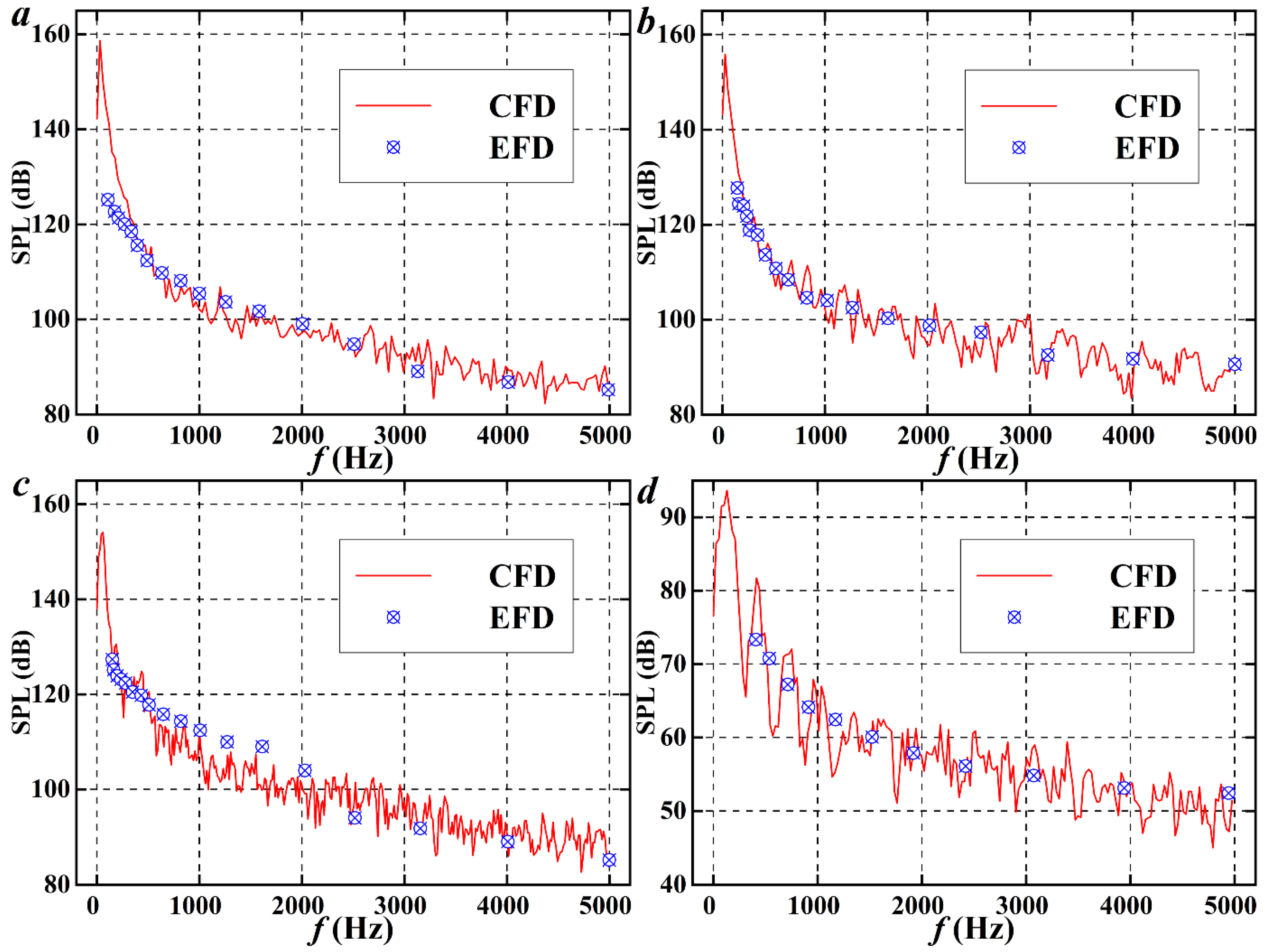
3.3.2. Noise Validation

Due to the difficulty in obtaining experimental noise data for the E1619 propeller, this paper verifies the accuracy of the acoustic calculation method using the noise experiments conducted by Lu et al. [50] and Jiang et al. [51] on the waterdrop-shaped AGSS-569 submarine in a large water channel. The submarine model, as shown in Figure 6a, adopts a water-droplet-type submarine model with a scale ratio of 1:25. The model length is L = 3.2 m, width is 0.4 m, and draft is 0.4 m. In the experiment, two swords were used to fix the model in the water tank test section, simulate the actual sailing speed of the model, and measure the noise sound pressure or fluctuating pressure at each point in the time domain. The water flow velocity was 5 m/s, and a single hydrophone was installed at 1.339 m directly below the submarine to measure the radiated noise at that point in this experiment. The computational domain is a cuboid with the flow direction set to 4L. The inflow length before the submarine is L, and the flow development length behind the submarine is 2L to ensure full wake development. Within the computational domain, a cylindrical permeable surface with a diameter of 1 m and a length of 6.8 m are set up to effectively capture the wake vortex structures of the submarine, thereby calculating the permeable surface integral information and ultimately obtaining the radiated noise characteristics. To accurately capture the near-wall flow information, the y⁺ is set to 1 when the flow velocity is 5 m/s, with a Reynolds number Re = 1.6 × 10⁷. The numerical simulation adopts unstructured trimmed grids to achieve good computational accuracy with a total of 4.86 million cells. The top and bottom boundaries are set as symmetry plane conditions, and the submarine surface is set as a no-slip wall condition. The computational domain and grid distribution for the submarine model are shown in Figure 6b and Figure 7, respectively.

Using the same numerical method as in Section 3.3.1, the hydrodynamic performance of the submarine is first simulated. Once the flow field stabilized, the FW-H acoustic model is added to further simulate the radiated noise from the submarine. Four hydrophones are placed around the submarine, numbered H1 to H4, with H1 to H3 installed on the submarine’s surface and H4 installed directly below the submarine. The specific parameters of each hydrophone position are provided in

Table 3. The position of experimental hydrophones.

Hydrophone	H1	H2	H3	H4
Coordinate	(0.4L, 180°)	(0.5L, 180°)	(0.65L, 180°)	(1.6 m, 0, −1.339 m)

. The experimental and simulation results of the surface and far-field hydrophones are compared in Figure 8. The sound pressure results are converted into the corresponding sound pressure level (SPL) using Equation (10), and the signals are transformed from the time domain into frequency domain for analysis.

$$SPL=10{\log }_{10}{\left(P_{rms}/P_{ref}\right)}^2,$$

(10)

where P_rms is the root mean square of sound pressure, and P_ref is the reference sound pressure in water, taken as 1 × 10⁻⁶ Pa. The noise spectrum characteristics on the submarine surface match well with the experimental data in low and medium frequency, and the broadband characteristics in high frequency also reflect the surface fluctuations of the submarine. The overall amplitude of the far-field noise aligns well with the experimental values. The validations using flow field and acoustic noise data confirm that the grid discretization strategy and numerical methods proposed in this paper are reliable, making them suitable for calculating the flow field and acoustic characteristics of the propeller.

4. Results and Analysis

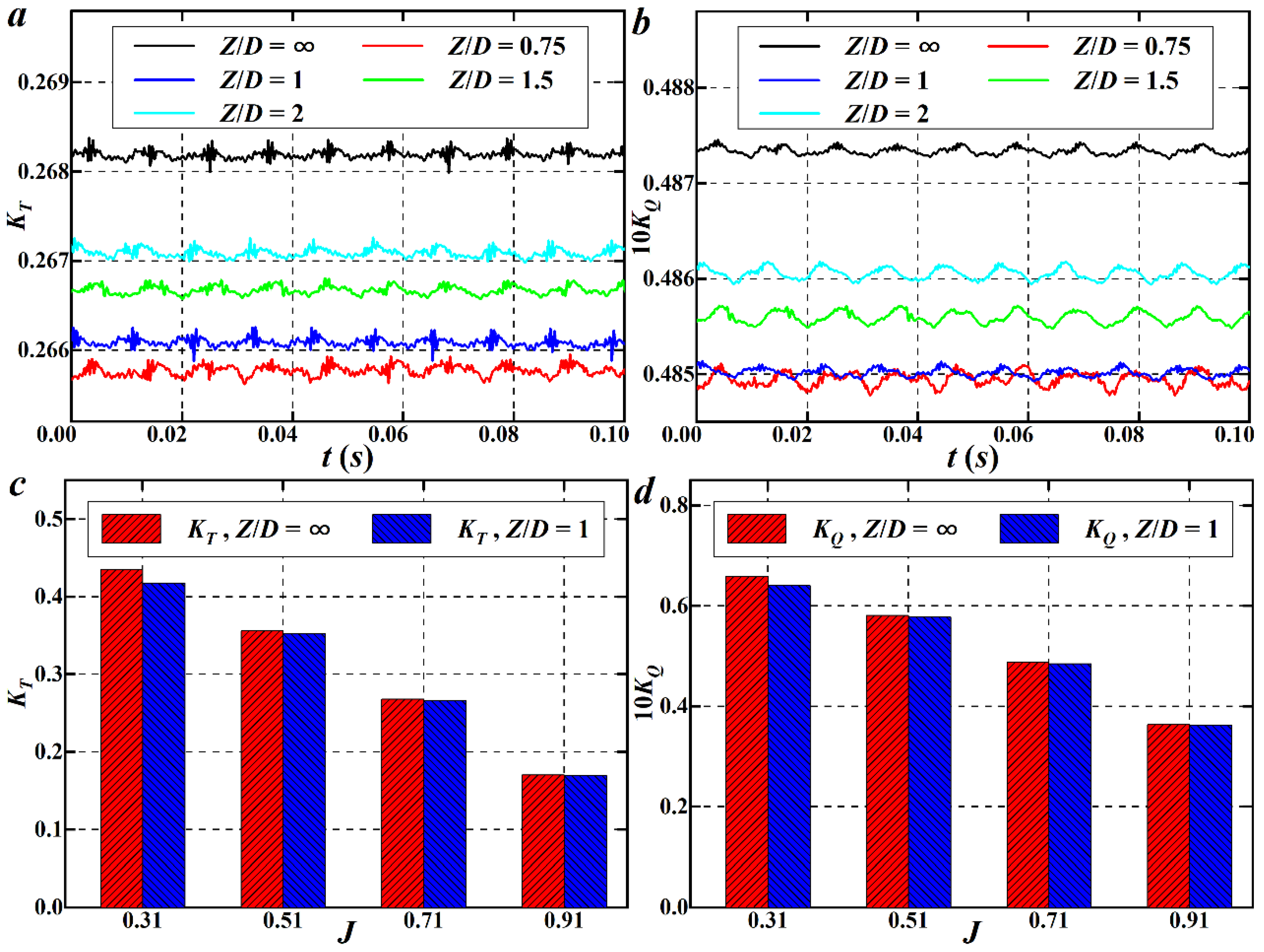
4.1. Global Parameters of Performance

In contrast to the infinite immerse depth condition, the free surface impacts the propeller’s inflow by increasing turbulence and causing a more uneven flow field. This results in fluctuations in thrust, torque, and efficiency. This study assesses the hydrodynamic and noise performance at an advance coefficient of J = 0.71 for four different immersion depths (Z/D = 0.75, 1, 1.5, and 2) and four advance coefficients (J = 0.31, 0.51, 0.71, and 0.91) at Z/D = 1. Figure 9a,b illustrate the time variations in K_T and K_Q for the propeller at J = 0.71 under varying immersion depths. In the absence of the free surface, K_T and K_Q display periodic fluctuations. However, with the free surface, K_T and K_Q are notably reduced. As Z increases, both K_T and K_Q progressively rise. The free surface also causes significant fluctuations in thrust and torque. To explore the changes in the wave pattern of free surface, flow field, and hydrodynamic characteristics of the propeller at different advance coefficients, numerical simulations are conducted for J = 0.31, 0.51, 0.71, and 0.91 at Z/D = 1. The advance coefficient changes with inflow speed, while the propeller’s rotational speed remains constant. Figure 9c,d present the average values of K_T and K_Q at the same immersion depth across different advance coefficients. At J = 0.31 and 0.51, the thrust and torque are considerably lower compared to those without the free surface. As J increases, the impact of the free surface on K_T and K_Q lessens, and at higher advance coefficients, the hydrodynamic performance approaches that without the free surface.

Table 4. The mean hydrodynamic performance of the propeller with different immersion depths at J = 0.71.

J = 0.71	KT	10KQ	η
Z/D = ∞	0.2682	0.4873	0.6219
Z/D = 0.75	0.2658	0.4849	0.6194
Z/D = 1	0.2661	0.4850	0.6200
Z/D = 1.5	0.2667	0.4856	0.6206
Z/D = 2	0.2671	0.4861	0.6209

compares the mean hydrodynamic performance of the propeller at various immersion depths. The results indicate that at the shallowest depth, Z/D = 0.75, K_T, K_Q, and η are lower than those observed without the free surface. As the depth increases, the free surface’s influence on thrust and torque fluctuations decreases rapidly. The reduction in torque is more significant than that in thrust, leading to increased open-water efficiency with depth. When Z/D = 2, the fluctuations due to free surface instability are much smaller, and the efficiency is closer to that without the free surface. Additionally, Figure 9a,b show that the amplitude of the time variations in thrust and torque decreases with increasing depth. This suggests that while strong fluctuations occur near the free surface, the overall periodic variation remains relatively stable.

Table 5. The reduction rates of K_T, K_Q, and η for the propeller with different advance coefficients at Z/D = 1.

Z/D = 1	KT/KT0	KQ/KQ0	η/η0
J = 0.31	0.9607	0.9727	0.9876
J = 0.51	0.9895	0.9940	0.9955
J = 0.71	0.9922	0.9953	0.9969
J = 0.91	0.9940	0.9964	0.9976

lists the reduction rates of K_T, K_Q, and η for the propeller at different advance coefficients with Z/D = 1. Here, K_T/K_T0, K_Q/K_Q0, and η/η₀ represent the ratios of thrust, torque, and efficiency for the propeller operating with free surface to those without it. The results show that as J increases, the reduction rates of thrust and torque decrease, while the reduction in blade surface load gradually increases. Since the reduction rate of thrust is smaller than that of torque, the open-water efficiency of the propeller increases with J. This indicates that the free surface’s impact on the propeller’s hydrodynamic performance diminishes at higher advance coefficients.

The power spectral density (PSD) of K_T for the propeller at different immersion depths and advance coefficients is shown in Figure 10. Across all conditions, a notable primary harmonic peak is observed at around 92 Hz. This peak results from changes in the blade’s angle of attack as it interacts with the incoming flow, as well as the momentum deficit caused by the interaction between the free surface and blades. Significant peaks are also present at blade harmonics, extending to a broadband peak around 1000 Hz. The dashed lines in the figure represent the isotropic homogeneous turbulence predicted by Kolmogorov theory, with a slope of −5/3. The current numerical simulations successfully capture the inertial frequency range under both conditions, demonstrating that the numerical model and mesh distribution are precise enough to accurately represent wake behavior throughout downstream evolution. The interaction between the free surface and propeller predominantly drives this effect, which decreases rapidly with increasing immersion depth, as shown in Figure 10a. The peak values in the low frequency gradually diminish. Due to the strong turbulence caused by the interaction between the blades and incoming flow, fluctuations decay significantly at high frequencies, although the overall peaks remain within the same order of magnitude. The low-frequency response of K_T varies significantly with different advance coefficients at a constant depth, as shown in Figure 10b. As expected, the spectral characteristics observed at J = 0.31 are significantly higher than those at other advance coefficients, with a more broadband characteristic observed at low frequency. This indicates that at low advance coefficients, the free surface substantially impacts the development of turbulent wakes, leading to more intense turbulent fluctuations. As J increases, this turbulent effect gradually weakens, and significant peak characteristics reappear around 92 Hz. However, the attenuation of high-frequency characteristics is more pronounced, with smaller amplitudes, indicating that free surface primarily affects broadband components near the peak blade frequency.

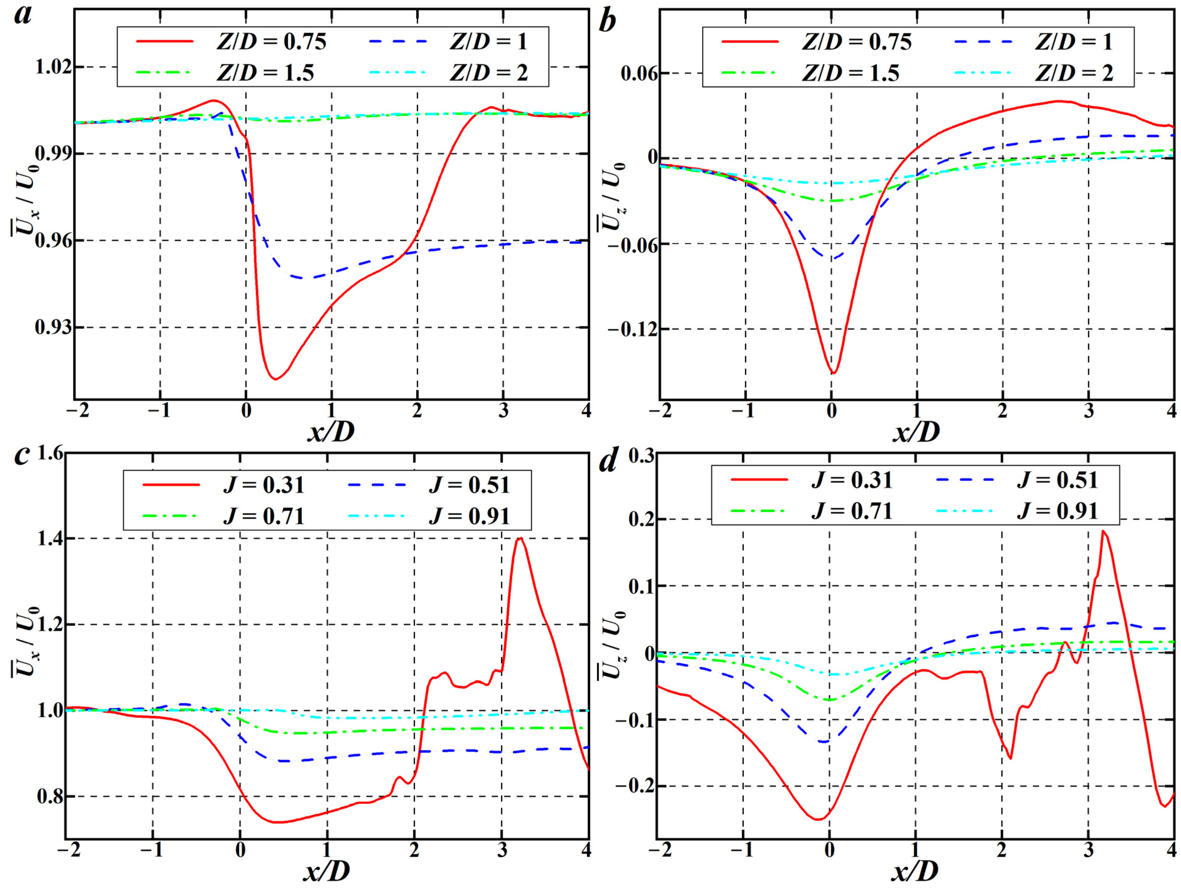
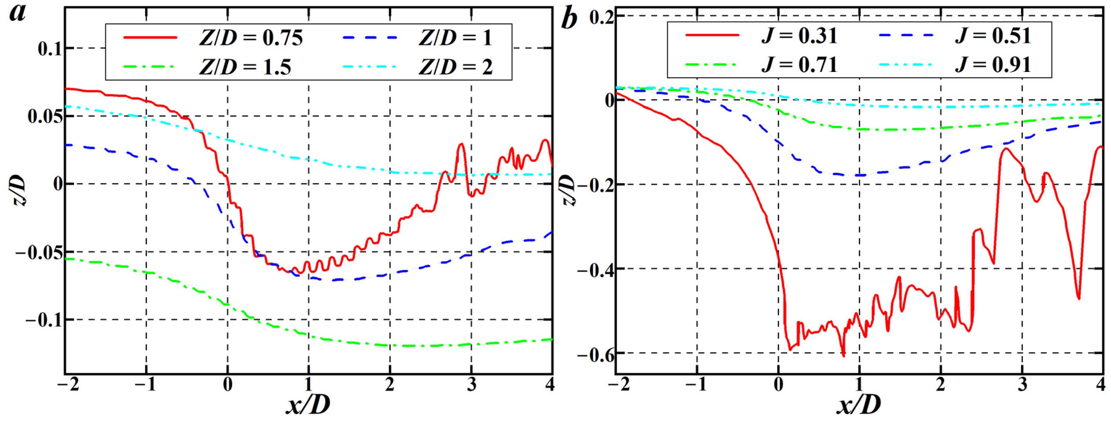
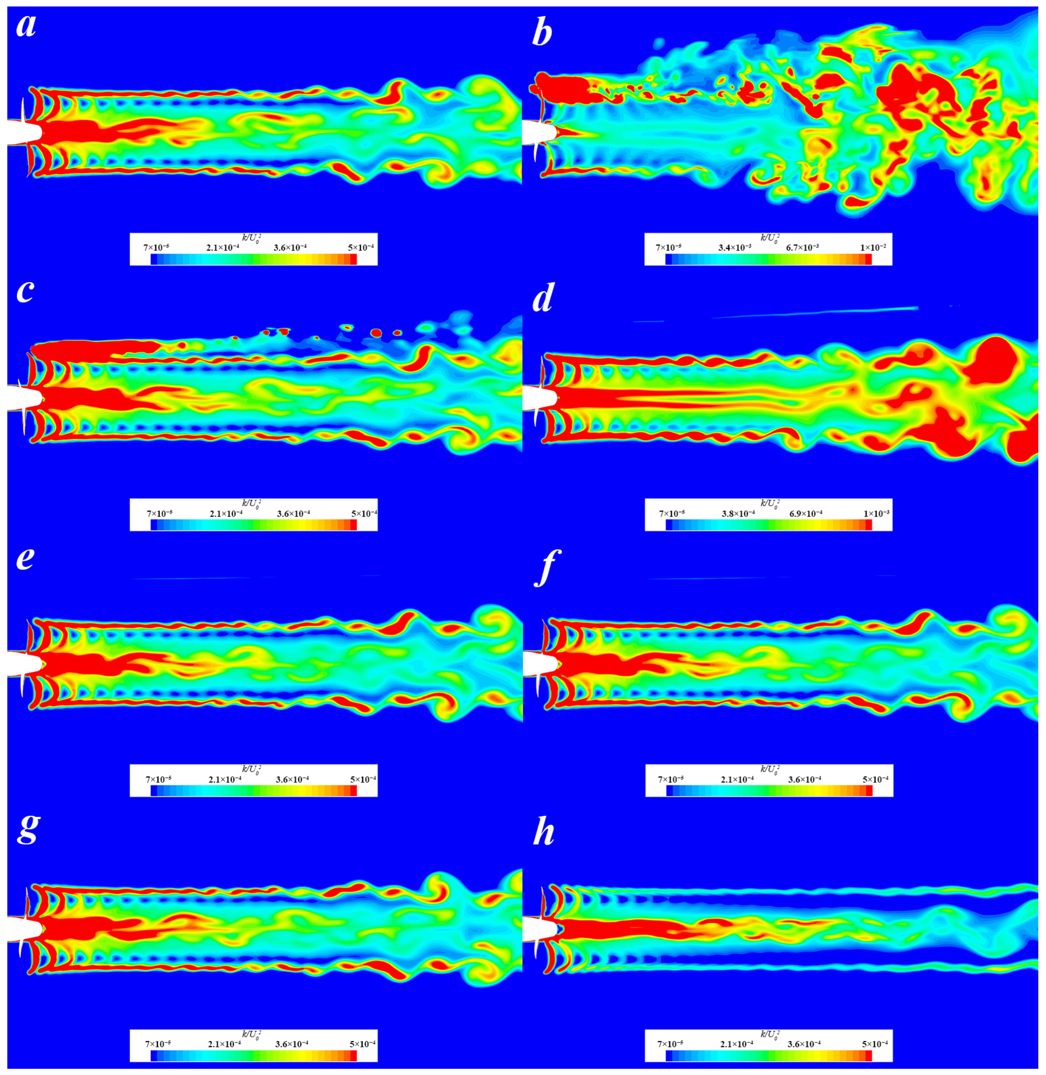
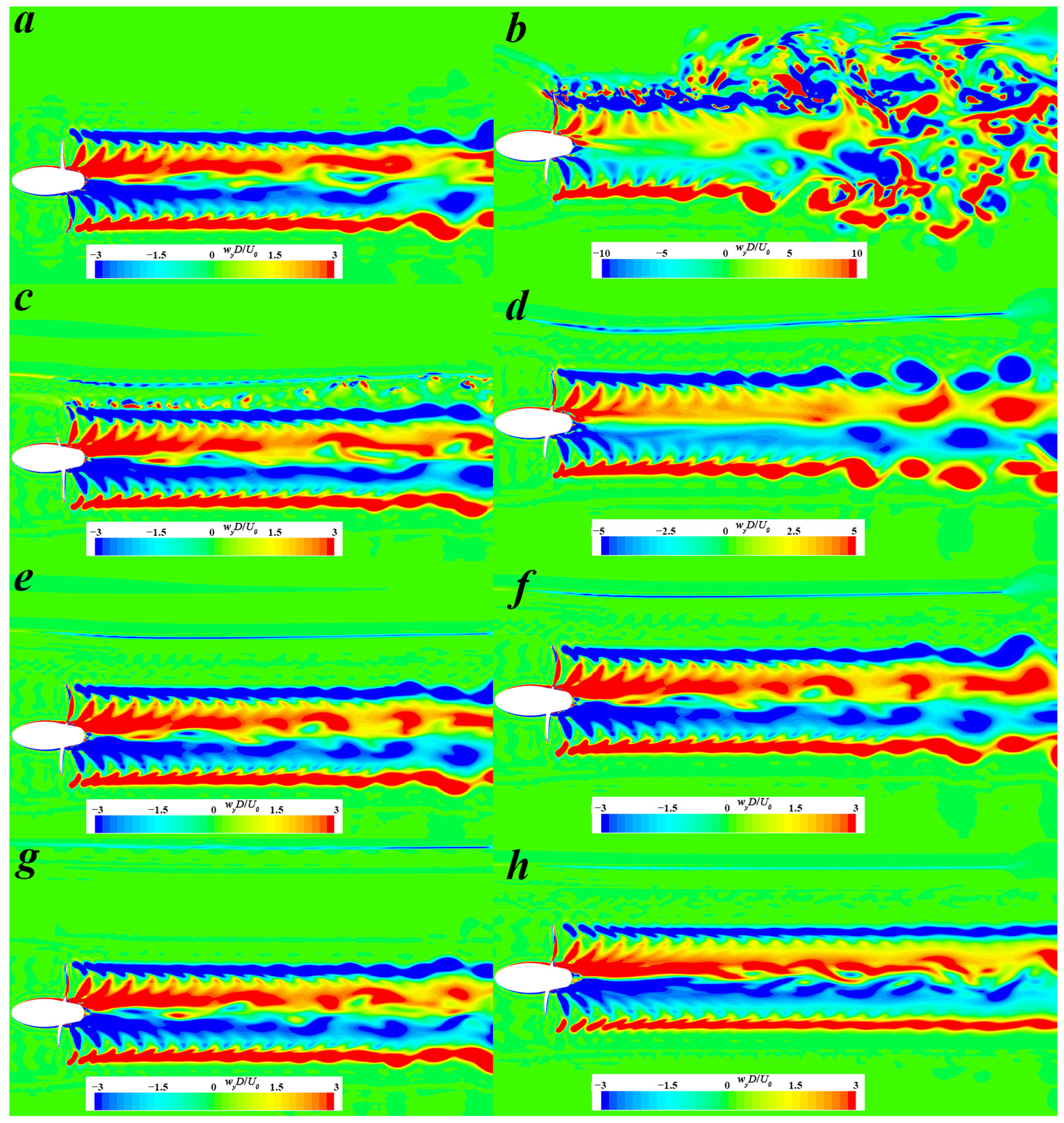
4.2. Flow Field Details

To better understand the effects of immersion depth and advance coefficient on flow kinematics, it is necessary to assess the variations in dimensionless mean axial and vertical velocity distributions in the wake relative to the dimensionless axial distance from the propeller. The velocity distributions at four immersion depths at y = 0 plane of free surface are illustrated in Figure 11a,b. At Z/D = 0.75 and 1, there is a significant velocity deficit in the downstream region within x/D = 0–1. As the depth increases, the velocity recovery is further delayed. At Z/D = 1.5 and 2, the peak velocity deficit quickly diminishes and recovers to the free-stream velocity. The vertical velocity shows a similar distribution pattern; at low immersion depths, the velocity deficit even becomes negative. As the depth increases, the velocity deficit gradually decreases, with the velocity gain in the downstream far wake also gradually reducing to zero due to free surface fluctuations. At the same immersion depth Z/D = 1, the axial velocity fluctuations at J = 0.31 are quite significant. The flow acceleration region is defined by the axial velocity, which corresponds to the velocity peaks illustrated in Figure 11c,d. The central wake causes extreme minimum and maximum values in the velocity profiles. As J increases, vortex strength decreases, and as the vortex system progresses downstream, its strength weakens. The sharp profiles of the axial velocity gradient become less pronounced, showing better propulsive performance at higher advance coefficients. Similarly, the fluctuations in vertical velocity exhibit a similar phenomenon, with the sharpness of the profile decreasing at higher advance coefficients due to the viscous attenuation of the tip and root vortices. Heydari and Sadat-Hosseini [52] reached similar conclusions in their analysis of propeller wakes.

The distributions of instantaneous dimensionless pressure coefficient $C_P={\displaystyle \frac{\overline{p}-p_{\infty }}{\frac{1}{2}\rho U_{\infty }^2}}$ (where $\overline{p}$ is the local pressure, and $p_{\infty }$ is the reference pressure at the same depth) on the propeller blade surfaces as a function of J are depicted in Figure 12, with the left side showing the suction sides and the right side showing the pressure sides. As illustrated in the axial and vertical velocity distributions in Figure 11, the significant pressure difference between the suction side and the pressure side at low advance coefficients results in strong tip vortices. This indicates that the axial thrust experienced by the propeller under heavy load conditions is greater, and the pressure difference decreases as the advance coefficient increases. At J = 0.31, due to the interaction with the free surface, C_P on the top blade is smaller than that on the bottom blade on the pressure side, while there is little difference on the suction side. This also leads to intense tip vortex shedding. At J = 0.51, this pressure non-uniformity has disappeared, but the pressure magnitude has significantly decreased, indicating the formation of a weaker vortex system. As J increases further, C_P on both sides of the blade become weak, and the overall pressure difference reduces, implying a diminished effect of the free surface on the propeller load and vortex structure.

Figure 13 compares the wave profiles at different immersion depths and advance coefficients at the y = 0 plane. At Z/D = 0.75, strong nonlinearity is observed at the wave peaks and troughs, due to significant fluctuations in the axial and vertical velocities within x/D = 0–3 in Figure 13a. The dimensionless wave profiles indicate that the free surface exhibits a transition from positive to negative wave height in front of and behind the propeller. At Z/D = 1, the wave pattern is similar to Z/D = 0.75, but with smaller wave heights, reflecting the weaker interaction between the propeller and the free surface. As Z increases, the overall wave height becomes negative, and at Z/D = 2, it turns positive, showing an asymmetric wave distribution. However, the further reduced fluctuation indicates a diminished effect of free surface and wake interference. The wave profiles along the centerline of the propeller at different advance coefficients are compared in Figure 13b. Strong nonlinear effects are observed at J = 0.31, with wave heights all below the initial free surface, corresponding to the large negative vertical velocities shown in Figure 11d. As J increases, the negative peak values of the wave height gradually decrease and get more subdued, eventually approaching the height of the initial free surface at high advance coefficients. This suggests that the influence of the free surface on the propeller becomes negligible at higher advance coefficients.

The contours of the free surface at various immersion depths and advance coefficients are compared in Figure 14, with all parameters being dimensionless. On the left side of the figure, the free surface exhibits typical Kelvin wave patterns. At smaller immersion depths, the wave height fluctuations are larger, especially downstream of the propeller wake. This shows a markedly different pattern compared to larger immersion depths, characterized by intense nonlinear wave phenomena. As the depth increases, this nonlinearity quickly disappears. The wave height reduction in the near-wake region becomes less significant, essentially recovering to the initial wave height at Z/D = 2. On the right side of Figure 14, the comparison of free surface wave patterns with varying advance coefficients shows that at J = 0.31, typical Kelvin waves and strong vortex structures in the entire flow field are observed. As J increases, the wave height decreases, and wave troughs appear behind the propeller. This can be attributed to the vertical velocity distributions in Figure 11. At lower advance coefficients, the suction surface at the top blade experiences strong negative vertical velocities, while the suction surface at the bottom blade exhibits strong positive vertical velocities, indicating the formation of tip vortices from the pressure surface to the suction surface. These tip vortices create alternating positive and negative vertical velocities downstream of the propeller, leading to alternating peaks and troughs in the wake, as explained by Paik [17] in his paper.

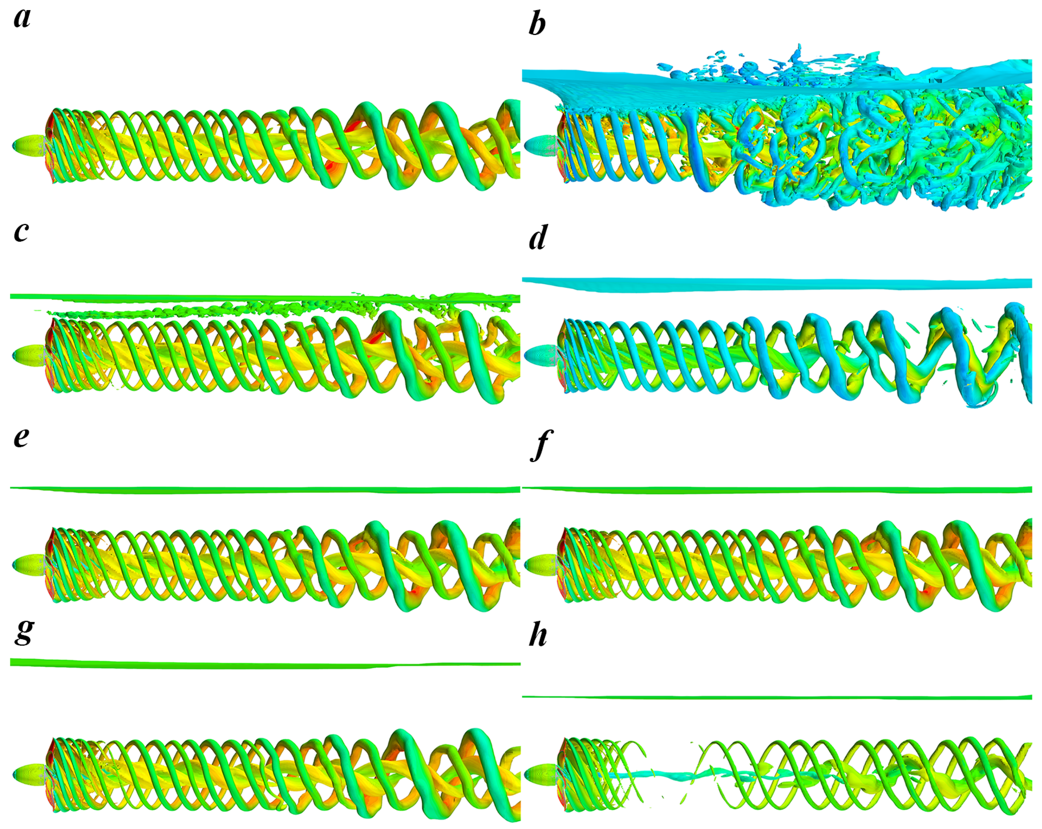
4.3. Vortex Structures

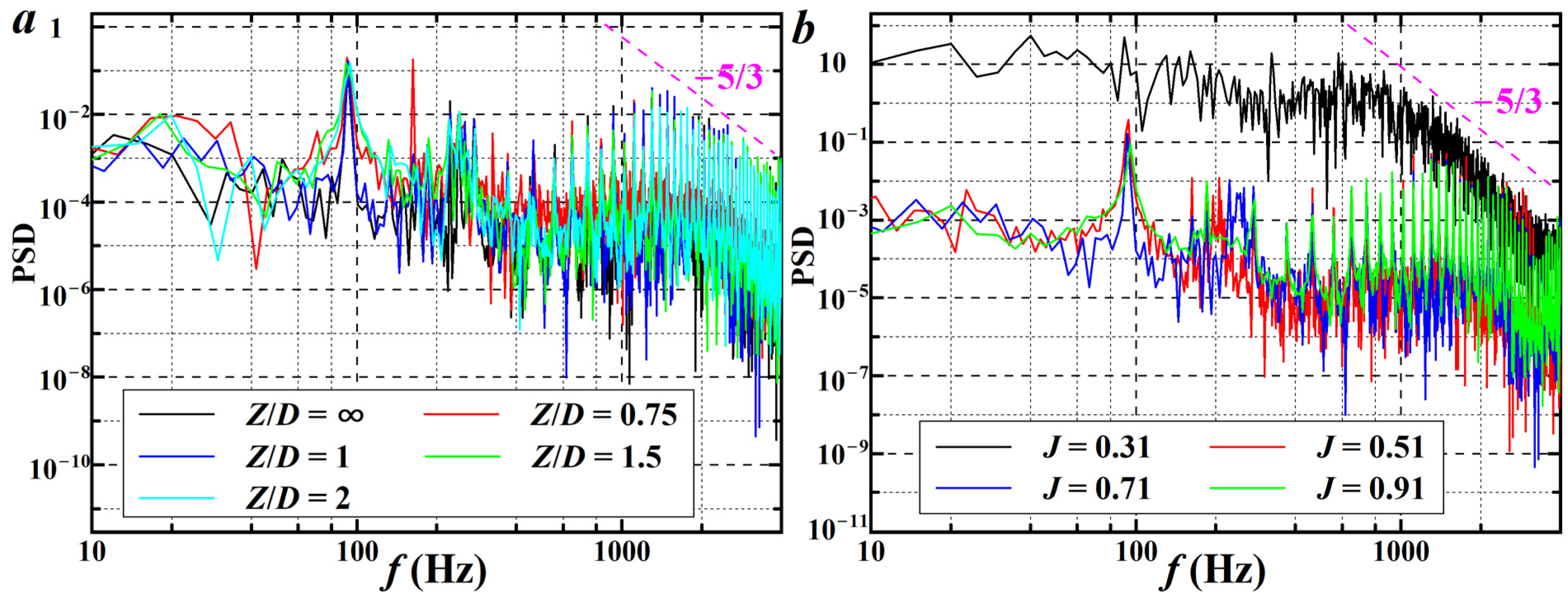
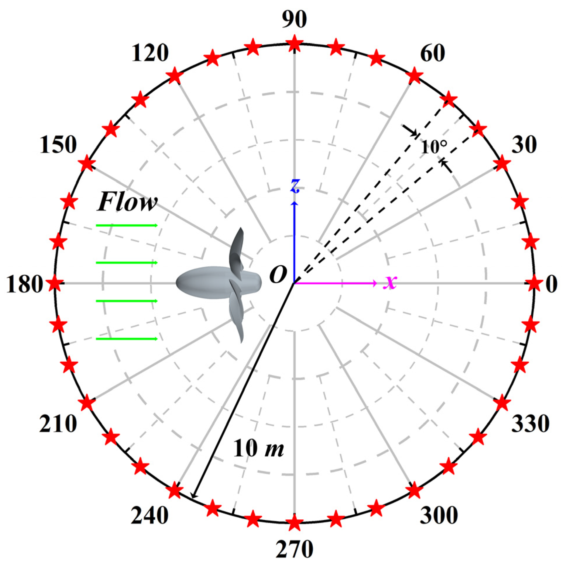
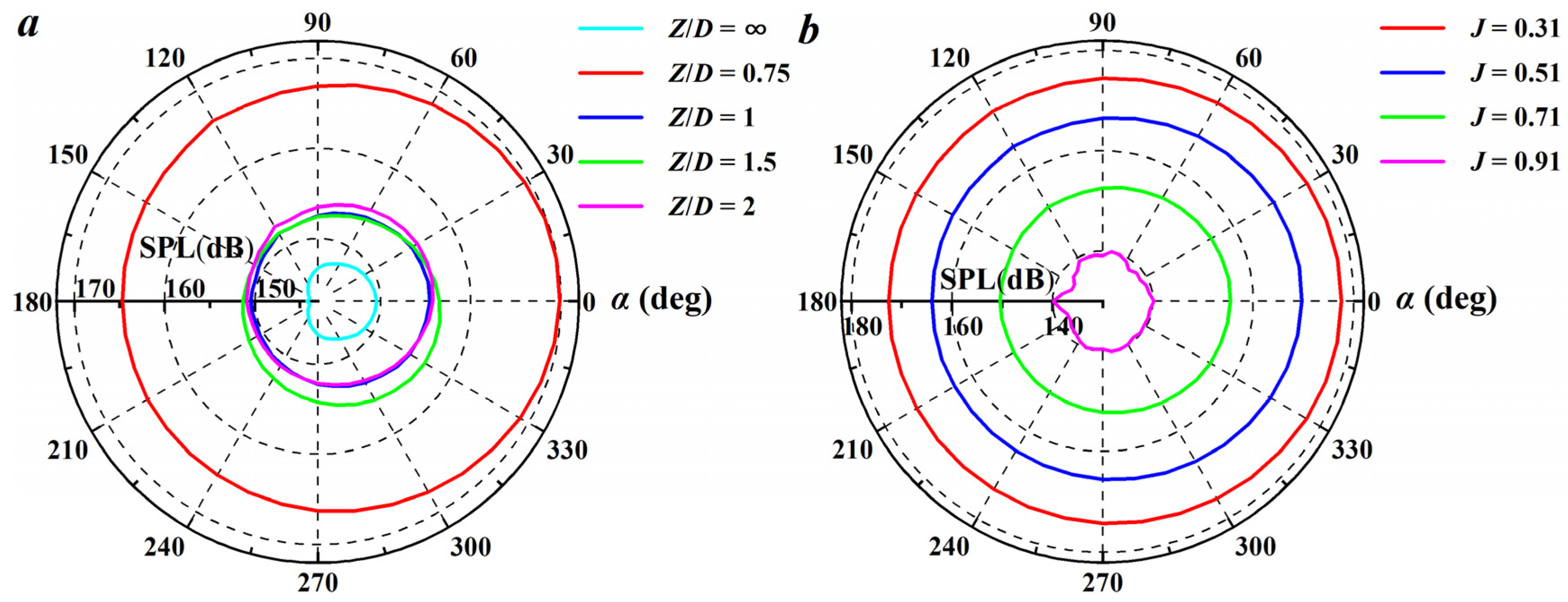
To gain a deeper understanding of the dynamics in the instantaneous propeller wake, the effects of immersion depth and advance coefficient on turbulence kinetic energy k are illustrated in Figure 15, rendered dimensionless using $U_0^2$. The gradient of k can infer the intensity of tip vortex cores and reveal the evolution of tip vortices under the influence of free surface. Compared to k without a free surface illustrated in the left side of Figure 15, k of the tip vortices at Z/D = 0.75 significantly increases at the blade tip and extends to the far-wake region, with no observable contraction of the tip vortices in the near field. This indicates that the proximity of the free surface to the propeller causes turbulence disruption in vortex structures, intensifying the tip vortex strength and fluctuation amplitude. As Z increases, paired vortex behavior due to mutual induction of vortex structures becomes observable in the middle region of the wake. The strength of the tip and hub vortices slightly decreases, indicating a reduction in blade load. The influence of the advance coefficient on turbulence kinetic energy is even more pronounced, as shown on the right side of Figure 15. At J = 0.31, the magnitude of k significantly increases and exhibits a more chaotic distribution, with instability appearing in the far field. This suggests that vortex structures under low-load conditions are strongly influenced by the free surface, severely altering the overall distribution of the flow field. As J increases, the overall distribution of the vortex structure gets closer to that without the free surface, and the energy in the wake decreases as the wake progresses. At high advance coefficients, compared to high-load conditions, the vortices near x/D = 1 exhibit paired behavior characterized by a weak and a strong vortex, followed by a diffusion process.

The impacts of immersion depth and advance coefficient on the instantaneous transverse vorticity field are demonstrated in Figure 16, illustrating the evolution trajectories of tip and hub vortices, dimensionless by D and U₀. On the left side of the figure, the vorticity distribution at different immersion depths is depicted. Without the free surface, the tip vortices in the near field are evenly distributed and exhibit a regular shape. As these vortices progress downstream, they become unstable, and the topology distorts and loses stability in the far field. At Z/D = 0.75, a series of continuous small-scale negative vorticities appear at the free surface, with paired adjacent vortices forming at the blade tip. These vortices become discontinuous with weaker strength as they move downstream, and interact significantly with the free surface, leading to a turbulent wake field. As Z increases, this intense interaction diminishes, and only elongated negative vortex structures are observed at the free surface. On the right side of Figure 16, the vorticity distributions for different advance coefficients are presented. At higher loads, the interaction between the free surface and the propeller wake vortices is extremely intense. In the near wake, neighboring vortices do not show paired or orderly development but rather transform into chaotic turbulence distribution. Particularly in the far wake, the interaction between the free surface, tip vortices, and hub vortices creates a mixed distribution of large- and small-scale vortex structures. This increases the blade load and affects structural strength. As J increases, the impact of free surface diminishes, and the wave patterns become smoother. The contraction of the tip vortices decreases due to the decrease in load. The pairing of tip vortices in the near wake becomes less distinct. Felli et al. [49] also discussed the vortex instability of propellers. At higher advance coefficients, the tip vortex cores are discrete and equidistant, aligning parallel to the propeller axis after initial contraction. The top region downstream of the tip vortex disappears due to the interaction with the free surface but extends further to the far wake, exhibiting stronger coherence, while the shape of the hub vortex shows a similar trend to the tip vortex.

The instantaneous vortex structures of the propeller wake are illustrated as iso-surfaces of Q = 1000 in Figure 17, with dimensionless axial velocity coloring. Without a free surface, the tip and hub vortices of the propeller alternate and develop in the wake, demonstrating strong coherence. At Z/D = 0.75, the interaction between the propeller and the free surface is most intense. The free surface not only generates significant fluctuations but also causes the tip vortex at the top of the propeller to be transmitted upward. This instability peaks in the far wake, leading to velocity deficits in the propeller wake and severely disrupting the vortex structures. As Z increases, the instability caused by the free surface weakens, with minimal differences between the vortices at the top and bottom of the propeller. The tip vortices remain stable downstream, although fluctuations at the free surface still persist. In the case of a higher propeller load J = 0.31, the interaction between the free surface and the propeller causes significant turbulence and fluctuations in the free surface height. The tip vortex structures are strong but gradually lose coherence, merging and distorting downstream to form large vortex tube structures. In the far wake, the vortex structures become larger and more chaotic, with vortex instability becoming more pronounced closer to the free surface and rapidly intensifying downstream. At J = 0.51, the local load at the top of the propeller decreases. However, compared to higher advance coefficients, the velocity of the tip vortex is relatively slower, and the tip vortices do not extend downstream. Although the interaction with the free surface weakens at high advance coefficients, the tip vortices are still clearly observable. Due to the weak intensity of the tip vortices, they dissipate early at J = 0.91, consistent with the observations of Felli et al. [49].

4.4. Radiated Noise

Building on the simulation method for the submarine model described in Section 3.3.1, noise calculations for the open-water propeller are conducted. The computational domain and grid discretization remain consistent with the hydrodynamic setup, and the results from hydrodynamic simulations are utilized as initial conditions for noise calculations. After the flow field stabilizes, the acoustic model is introduced. To capture fluctuations of the propeller surface and flow field accurately, a permeable surface is adopted as the sound source surface. A series of acoustic monitoring points are uniformly distributed in Figure 18. With the propeller’s center as the origin, 36 virtual hydrophones are evenly arranged on a circle with a 10 m radius at y = 0 plane. Each pair of adjacent hydrophones on the plane is separated by 10°. The calculation is then carried out until convergence. The total sound pressure data (combining loading and thickness sound pressure) at the hydrophones are obtained. The time-domain data of sound pressure are transformed into the corresponding sound pressure level through Fourier transform.

The frequency spectra of sound pressure fluctuations at the 0° hydrophone under various immersion depths and advance coefficients are shown in Figure 19. All conditions exhibit periodic fluctuations in sound pressure of different hydrophones. Since the propeller radiated noise consists of discrete tonal noise at axis and blade frequencies and their harmonics, as well as broadband noise, the spectral characteristics are rich. Several peaks are visible within the 20–1000 Hz range, with a linear decay trend. At shallow immersion depths, the sound pressure amplitude increases significantly and does not show prominent tonal characteristics in Figure 19a. With increasing Z, the low-frequency tonal features gradually recover, and the maximum peak decreases, although it remains higher than that without the free surface. The overall amplitude of the broadband spectrum is less affected, but the fluctuation level remains high due to the interaction between the free surface and the propeller. At J = 0.31 with a high-load condition, the fluctuating pressure is very significant, as shown in Figure 17b. Therefore, the sound pressure levels in the 20–5000 Hz range are high and rapidly decrease after reaching the maximum peak in Figure 19b. As the load decreases, the spectral peaks gradually diminish, with a significant reduction in the maximum peak with increasing J. Further increase in the advance coefficient has less impact on broadband noise characteristics, mainly affecting the reduction in low-frequency tonal noise. This indicates that the free surface significantly affects propeller noise at various advance coefficients.

The directivity patterns of sound pressure for the propeller at the y = 0 plane under different free surface conditions can be observed in Figure 20. In the absence of a free surface, the directivity exhibits an “elliptical” distribution with clear symmetry in the vertical planes, as shown in Figure 20a. The maximum sound pressure is located behind the propeller wake, indicating that turbulent fluctuations caused by the vortex structures are the primary source of noise. At shallow immersion depths, the magnitude of the noise directivity increases significantly, by 20 dB compared to that with no free surface. The strong interaction between the free surface and tip vortices causes the directivity to shift towards the rear. As Z increases, the noise decreases significantly. Due to varying peak-to-trough amplitudes at different immersion depths, some asymmetry in the directivity is observed in the vertical planes. However, the overall SPL is less affected by immersion depth. The influence of advance coefficient on noise is more pronounced. Higher propeller loads result in higher sound pressure levels, and the reduction in noise with increasing J is quite significant. At J = 0.91, the directivity is more prominent both in front of and behind the propeller, demonstrating that the free surface also affects the distribution of directivity at low loads.

5. Conclusions

Numerical simulation methods were adopted to analyze the hydrodynamic and noise characteristics of the open-water propeller E1619 near the free surface in this paper. By comparing with experimental values, the open-water performance of the propeller was validated. The accuracy of the numerical method was confirmed by further validating the noise calculation results with a submarine model. To demonstrate the effects of a free surface on the propeller, numerical simulations were performed for the propeller at four different immersion depths and advance coefficients.

The results indicate that the interaction between the propeller and the free surface significantly affects propeller thrust and torque, especially at shallow immersion depths, where the loads on the upper blades near the free surface are much greater. Strong free surface fluctuations at shallow depths also cause instability and breakdown of tip vortices in the near field, as evidenced by the fluctuations in axial and vertical velocities. As the immersion depth increases, the effects of the free surface on the hydrodynamic performance gradually diminish, and efficiency gradually recovers to that without the free surface. The amplitude of wave height on the free surface decreases, and the instability of the wake vortex structure gradually disappears, indicating a significant reduction in the impact of the free surface.

At lower advance coefficients, there was a notable increase in fluctuations of thrust and torque, accompanied by a decrease in propeller efficiency. The Kelvin wave pattern of the free surface was clearly observed, with wake instability occurring closer to the propeller plane and more pronounced vortex merging in the upper part of the wake. As the advance coefficient increases, the reduction in thrust and torque becomes more significant, and the interaction between free surface waves and tip vortices gradually diminishes. At higher advance coefficients, due to the weak tip vortices, they dissipate early in the near wake.

The spectral characteristics and directivity distribution of the radiated noise also validated the variations in hydrodynamic performance. At shallow immersion depths and low advance coefficients, the overall sound pressure levels in the propeller spectrum were significant. The directivity distribution indicates that turbulence instability leads to a higher noise level throughout the entire flow field. As the immersion depth and advance coefficient increased, the noise level gradually decreased. However, due to the presence of the free surface, the sound pressure level remained higher than that without the free surface. The results indicate that the immersion depth and advance coefficient have a significant impact on the hydrodynamic and noise characteristics of the propeller operating near the free surface.

The current research adopted a propeller model in open water with a uniform inflow, primarily providing theoretical support for specific parameter optimization, but it did not fully transition into actual design. However, this preliminary research lays the foundation for future analysis of more complex wake fields and free surface effects. In future work, the wake and actual operating conditions of ships will be included in the research scope, further refining the propeller design and noise prediction to improve the model’s practical applicability and optimize the ship design to better meet the specific needs of surface vessels and submarines.

References

1. Wang, L.Z.; Guo, C.Y.; Wan, L.; Su, Y.M. Numerical analysis of propeller during heave motion near a free surface. Mar. Technol. Soc. J. 2017, 51, 40–51. [Google Scholar]
2. Mascio, D.A.; Dubbioso, G.; Muscari, R. Vortex structures in the wake of a marine propeller operating close to a free surface. J. Fluid Mech. 2022, 949, A33. [Google Scholar] [CrossRef]
3. Orihara, H.; Miyata, H. Evaluation of added resistance in regular incident waves by computational fluid dynamics motion simulation using an overlapping grid system. J. Mar. Sci. Technol. 2003, 8, 47–60. [Google Scholar] [CrossRef]
4. Arribas, F.P. Some methods to obtain the added resistance of a ship advancing in waves. Ocean Eng. 2007, 34, 946–955. [Google Scholar] [CrossRef]
5. Sadat-Hosseini, H.; Wu, P.C.; Carrica, P.M.; Kim, H.; Toda, Y.; Stern, F. CFD verification and validation of added resistance and motions of KVLCC2 with fixed and free surge in short and long head waves. Ocean Eng. 2013, 59, 240–273. [Google Scholar] [CrossRef]
6. Chuang, Z.; Steen, S. Prediction of speed loss of a ship in waves. In Proceedings of the Second International Symposium on Marine Propulsors smp, Hamburg, Germany, 15–17 June 2011; Volume 11, pp. 24–32. [Google Scholar]
7. Ueno, M.; Tsukada, Y.; Tanizawa, K. Estimation and prediction of effective inflow velocity to propeller in waves. J. Mar. Sci. Technol. 2013, 18, 339–348. [Google Scholar] [CrossRef]
8. Yu, D.; Wang, L.; Liu, H.; Cui, M. Influence of Load Conditions on the Propeller Wake Evolution. J. Mar. Sci. Eng. 2023, 11, 1674. [Google Scholar] [CrossRef]
9. Sun, P.; Pan, L.; Liu, W.; Zhou, J.; Zhao, T. Wake characteristic analysis of a marine propeller under different loading conditions in coastal environments. J. Coast. Res. 2022, 38, 613–623. [Google Scholar] [CrossRef]
10. Zhou, J.; Sun, P.; Pan, L. Modal analysis of the wake instabilities of a propeller operating in coastal environments. J. Coast. Res. 2022, 38, 1163–1171. [Google Scholar] [CrossRef]
11. Gong, J.; Guo, C.Y.; Zhao, D.G.; Wu, T.C.; Song, K.W. A comparative DES study of wake vortex evolution for ducted and non-ducted propellers. Ocean Eng. 2018, 160, 78–93. [Google Scholar] [CrossRef]
12. Chase, N. Simulations of the DARPA Suboff Submarine Including Self-Propulsion with the E1619 Propeller. Master’s Thesis, University of Iowa, Iowa City, IA, USA, 2012. [Google Scholar]
13. Wang, L.; Liu, X.; Guo, J.; Li, M.; Liao, J. The dynamic characteristics in the wake systems of a propeller operating under different loading conditions. Ocean Eng. 2023, 286, 115518. [Google Scholar] [CrossRef]
14. Baek, D.G.; Yoon, H.S.; Jung, J.H.; Kim, K.S.; Paik, B.G. Effects of the advance ratio on the evolution of a propeller wake. Comput. Fluids 2015, 118, 32–43. [Google Scholar] [CrossRef]
15. Kozlowska, A.M.; Steen, S.; Koushan, K. Classification of different type of propeller ventilation and ventilation inception mechanism. In Proceedings of the First International Symposium on Marine Propulsors, Trondheim, Norway, 22–24 June 2009; pp. 22–24. [Google Scholar]
16. Kozlowska, A.M.; Wöckner, K.; Steen, S.; Rung, T.; Koushan, K.; Spence, S. Numerical and experimental study of propeller ventilation. In Proceedings of the Second International Symposium on Marine Propulors, Hamburg, Germany, 15–17 June 2011. [Google Scholar]
17. Paik, K.J. Numerical study on the hydrodynamic characteristics of a propeller operating beneath a free surface. Int. J. Nav. Archit. Ocean Eng. 2017, 9, 655–667. [Google Scholar] [CrossRef]
18. Califano, A.; Steen, S. Numerical simulations of a fully submerged propeller subject to ventilation. Ocean Eng. 2011, 38, 1582–1599. [Google Scholar] [CrossRef]
19. Paik, B.G.; Lee, J.Y.; Lee, S.J. Effect of propeller immersion depth on the flow around a marine propeller. J. Ship Res. 2008, 52, 102–113. [Google Scholar]
20. Wang, L.; Martin, J.E.; Felli, M.; Carrica, P.M. Experiments and CFD for the propeller wake of a generic submarine operating near the surface. Ocean Eng. 2020, 206, 107304. [Google Scholar] [CrossRef]
21. Lungu, A. A DES-based study of the flow around the self-propelled DARPA Suboff working in deep immersion and beneath the free-surface. Ocean Eng. 2022, 244, 110358. [Google Scholar] [CrossRef]
22. Yu, M.S.; Wu, Y.S.; Pang, Y.Z. A review of progress for hydrodynamic noise of ships. J. Ship Mech. 2007, 11, 152–158. [Google Scholar]
23. Leaper, R.; Renilson, M.; Ryan, C. Reducing underwater noise from large commercial ships: Current status and future directions. J. Ocean Technol. 2014, 9, 51. [Google Scholar]
24. Carlton, J. Marine Propellers and Propulsion; Butterworth-Heinemann: Oxford, UK, 2018. [Google Scholar]
25. Sezen, S.; Atlar, M. Marine propeller underwater radiated noise prediction with the FWH acoustic analogy part 3: Assessment of full-scale propeller hydroacoustic performance versus sea trial data. Ocean Eng. 2022, 266, 112712. [Google Scholar] [CrossRef]
26. Özden, M.C.; Gürkan, A.Y.; Özden, Y.A.; Canyurt, T.G.; Korkut, E. Underwater radiated noise prediction for a submarine propeller in different flow conditions. Ocean Eng. 2016, 126, 488–500. [Google Scholar] [CrossRef]
27. Chen, Y.W.; Pan, C.C.; Lin, Y.H.; Shih, C.F.; Shen, J.H.; Chang, C.M. Acoustic Field Radiation Prediction and Verification of Underwater Vehicles under a Free Surface. J. Mar. Sci. Eng. 2023, 11, 1940. [Google Scholar] [CrossRef]
28. Ross, D.; Kuperman, W. Mechanics of Underwater Noise; Acoustical Society of America: Melville, NY, USA, 1989. [Google Scholar]
29. Burella, G.; Moro, L.; Colbourne, B. Noise sources and hazardous noise levels on fishing vessels: The case of newfoundland and Labrador’s fleet. Ocean Eng. 2019, 173, 116–130. [Google Scholar] [CrossRef]
30. Farkas, A.; Degiuli, N.; Martić, I.; Dejhalla, R. Numerical and experimental assessment of nominal wake for a bulk carrier. J. Mar. Sci. Technol. 2019, 24, 1092–1104. [Google Scholar] [CrossRef]
31. Wilcox, D.C. Turbulence Modeling for CFD; DCW Industries, Incorporated: La Canada, CA, USA, 1994; Volume 2, pp. 103–217. [Google Scholar]
32. Spalart, P.R. Comments on the Feasibility of LES for Wings and on the Hybrid RANS/LES Approach. In Proceedings of the First AFOSR International Conference on DNS/LES Ruston, LA, USA, 4–8 August 1997; pp. 137–147. [Google Scholar]
33. Menter, F.R. Two-equation eddy-viscosity turbulence models for engineering applications. AIAA J. 1994, 32, 1598–1605. [Google Scholar] [CrossRef]
34. Guo, H.; Guo, C.; Hu, J.; Zhang, W. Wake-structure interaction of flow over a freely rotating hydrofoil in the wake of a cylinder. J. Fluids Struct. 2023, 119, 103891. [Google Scholar] [CrossRef]
35. Zhang, J.; Gidado, F.; Adamu, A.; He, K.; Krajnović, S.; Gao, G. Assessment of URANS, SAS, and IDDES on the bi-stable wake flow of a generic ship. Ocean Eng. 2023, 286, 115625. [Google Scholar] [CrossRef]
36. Guo, H.; Li, G.; Zou, Z. Numerical simulation of the flow around NACA0018 airfoil at high incidences by using RANS and DES methods. J. Mar. Sci. Eng. 2022, 10, 847. [Google Scholar] [CrossRef]
37. Posa, A.; Broglia, R.; Shi, W.; Mario, F. Large eddy simulation of a marine propeller with leading edge tubercles. Phys. Fluids 2024, 36, 115148. [Google Scholar] [CrossRef]
38. He, K.; Su, X.; Gao, G.; Krajnović, S. Evaluation of LES, IDDES and URANS for prediction of flow around a streamlined high-speed train. J. Wind Eng. Ind. Aerodyn. 2022, 223, 104952. [Google Scholar] [CrossRef]
39. Lighthill, M.J. On sound generated aerodynamically I. General theory. Proc. R. Soc. Lond. A 1952, 211, 564–587. [Google Scholar]
40. Zhou, B.Y.; Albring, T.A.; Gauger, N.R.; Economon, T.D.; Palacios, F.; Alonso, J.J. A discrete adjoint framework for unsteady aerodynamic and aeroacoustic optimization. In Proceedings of the 16th AIAA/ISSMO Multidisciplinary Analysis and Optimization Conference, Dallas, TX, USA, 22–26 June 2015; p. 3355. [Google Scholar]
41. Zhou, B.Y.; Albring, T.; Gauger, N.R.; Ilario da Silva, C.R.; Economon, T.D.; Alonso, J.J. A discrete adjoint approach for jet-flap interaction noise reduction. In Proceedings of the 58th AIAA/ASCE/AHS/ASC Structures, Structural Dynamics, and Materials Conference, Grapevine, TX, USA, 9–13 January 2017; p. 0130. [Google Scholar]
42. Choi, W.S.; Choi, Y.; Hong, S.Y.; Song, J.H.; Kwon, H.W.; Jung, C.M. Turbulence-induced noise of a submerged cylinder using a permeable FW–H method. Int. J. Nav. Archit. Ocean Eng. 2016, 8, 235–242. [Google Scholar] [CrossRef]
43. Farassat, F.; Brentner, K.S. Supersonic quadrupole noise theory for high-speed helicopter rotors. J. Sound Vib. 1998, 218, 481–500. [Google Scholar] [CrossRef]
44. Wang, L.; Wu, T.; Gong, J.; Yang, Y. Numerical analysis of the wake dynamics of a propeller. Phys. Fluids 2021, 33, 095120. [Google Scholar] [CrossRef]
45. Guo, H.; Guo, C.; Hu, J.; Lin, J.; Zhong, X. Influence of jet flow on the hydrodynamic and noise performance of propeller. Phys. Fluids 2021, 33, 065123. [Google Scholar] [CrossRef]
46. Felice, D.F.; Felli, M.; Liefvendahl, M.; Svennberg, U. Numerical and experimental analysis of the wake behavior of a generic submarine propeller. Prism 2009, 1, 158. [Google Scholar]
47. Chase, N.; Carrica, P.M. Submarine propeller computations and application to self-propulsion of DARPA Suboff. Ocean Eng. 2013, 60, 68–80. [Google Scholar] [CrossRef]
48. Rodriguez, S. Applied Computational Fluid Dynamics and Turbulence Modeling. In Practical Tools, Tips and Techniques; Springer Nature: Berlin, Germany, 2019. [Google Scholar]
49. Felli, M.; Camussi, R.; Felice, D.F. Mechanisms of evolution of the propeller wake in the transition and far fields. J. Fluid Mech. 2011, 682, 5–53. [Google Scholar] [CrossRef]
50. Lu, Y.; Zhang, H.; Pan, X. Comparison between the simulations of flow-noise of a submarine-like body with four different turbulent models. Chin. J. Hydrodyn. 2008, 23, 348–355. [Google Scholar]
51. Jiang, W.C.; Zhang, H.X.; Meng, K.Y. Research on the flow noise of underwater submarine based on boundary element method. Chin. J. Hydrodyn. 2013, 28, 453–459. [Google Scholar]
52. Heydari, M.; Sadat-Hosseini, H. Analysis of propeller wake field and vortical structures using k − ω SST Method. Ocean Eng. 2020, 204, 107247. [Google Scholar] [CrossRef]
Figure 1. E1619 propeller and its associated reference framework are shown in two views: (a) oblique view and (b) side view.
Jmse 12 02208 g001
Figure 2. The setup and boundary conditions of the infinite depth computational domain.
Jmse 12 02208 g002
Figure 3. Grid discretization of the computational domain: (a) tip vortex and wake refinements in the wake, (b) grid distribution near the propeller boundary layer.
Jmse 12 02208 g003
Figure 4. The simulation results of the open-water performance of the propeller at different inflow velocities compared with the experimental values.
Jmse 12 02208 g004
Figure 5. The vorticity magnitude at plane y = 0 of the simulation results (a) reproduced from Chase and Carrica [47], with permission from Ocean Engineering, 2013, compared with those (b) in this study.
Jmse 12 02208 g005
Figure 6. (a) The geometric model of the AGSS-569 submarine, and (b) the computational domain and boundary conditions for the submarine model.
Jmse 12 02208 g006
Figure 7. The grid refinements of the boundary layer and wake for the submarine model.
Jmse 12 02208 g007
Figure 8. Comparison of sound pressure level of hydrophones by experiment and numerical simulation. (a) H1, (b) H2, (c) H3, and (d) H4.
Jmse 12 02208 g008
Figure 9. The time variations in (a) KT and (b) KQ for the propeller at J = 0.71 under different immersion depths, and the average values of (c) KT and (d) KQ at Z/D = 1 against different advance coefficients.
Jmse 12 02208 g009
Figure 10. The power spectral density of KT for the propeller at different (a) immersion depths and (b) advance coefficients.
Jmse 12 02208 g010
Figure 11. The dimensionless mean (a,c) axial and (b,d) vertical velocity distributions at y = 0 plane of free surface with (a,b) different immersion depths and (c,d) advance coefficients.
Jmse 12 02208 g011
Figure 12. Contours of instantaneous dimensionless pressure on (a,c,e,g) suction sides and (b,d,f,h) pressure sides for (a,b) J = 0.31, (c,d) J = 0.51, (e,f) J = 0.71, and (g,h) J = 0.91.
Jmse 12 02208 g012
Figure 13. The wave profiles at different (a) immersion depths and (b) advance coefficients at y = 0 plane.
Jmse 12 02208 g013
Figure 14. Contours of free surface at different immersion depths: (a) Z/D = 0.75, (c) Z/D = 1, (e) Z/D = 1.5, (g) Z/D = 2; and advance coefficients: (b) J = 0.31, (d) J = 0.51, (f) J = 0.71, and (h) J = 0.91.
Jmse 12 02208 g014
Figure 15. Contours of dimensionless turbulence kinetic energy at different immersion depths: (a) Z/D = ∞, (c) Z/D = 0.75, (e) Z/D = 1, (g) Z/D = 1.5; and advance coefficients: (b) J = 0.31, (d) J = 0.51, (f) J = 0.71, and (h) J = 0.91.
Jmse 12 02208 g015
Figure 16. Contours of instantaneous transverse vorticity at different immersion depths: (a) Z/D = ∞, (c) Z/D = 0.75, (e) Z/D = 1, (g) Z/D = 1.5, and advance coefficients: (b) J = 0.31, (d) J = 0.51, (f) J = 0.71, and (h) J = 0.91.
Jmse 12 02208 g016
Figure 17. The propeller wake vortex system presented by Q-criterion (Q = 1000) at different immersion depths: (a) Z/D = ∞, (c) Z/D = 0.75, (e) Z/D = 1, (g) Z/D = 1.5, and advance coefficients: (b) J = 0.31, (d) J = 0.51, (f) J = 0.71, and (h) J = 0.91.
Jmse 12 02208 g017
Figure 18. Location of directivity hydrophones uniformly distributed on a circle with a 10 m radius at y = 0 plane.
Jmse 12 02208 g018
Figure 19. The frequency spectra of sound pressure fluctuations at the 0° hydrophone under different (a) immersion depths and (b) advance coefficients.
Jmse 12 02208 g019
Figure 20. The directivity patterns of sound pressure for the propeller at y = 0 plane under different (a) immersion depths and (b) advance coefficients.
Jmse 12 02208 g020