Three-Dimensional Numerical Modeling of Local Scour Around Bridge Foundations Based on an Improved Wall Shear Stress Model

Abstract

Currently, there are two primary issues with CFD simulations of local scour around bridge foundations using the RANS method. Firstly, the self-sustaining characteristics of turbulent boundary conditions at the inlet require special attention. Secondly, the simulated location of the maximum scour depth does not align with experimental observations. This paper employs the RANS method to model the hydrodynamic characteristics surrounding bridge piers. The sediment transport model and sediment-sliding model, considering any slope of the riverbed, were adopted to simulate the spatiotemporal evolution of local scour around the bridge foundation. Building on traditional methods and assuming local turbulence equilibrium, a self-sustaining model is theoretically derived. This model swiftly develops a balanced turbulent boundary layer, achieving a horizontally uniform flow field and effectively maintaining consistency between the inlet-given turbulent profile and physical reality. Additionally, by incorporating the velocity component of the downward-flow in front of the pier and the average shear stress around the pier into the excess shear stress model, the refined wall shear stress model accurately estimates the scouring contributions of the downward-flow and the horseshoe vortex system in this region. The numerical results including the maximum scour depth, location, and scour pit shape are consistent with experimental findings. The findings demonstrate that the numerical approach proposed in this study effectively addresses the issue of inadequate estimation of turbulent characteristics in scour pit at the leading edge of bridge piers using the RANS method. This method offers novel insights and approaches for addressing local scour issues in bridges and offshore wind turbines, as well as vortex-induced vibration issues in submarine pipelines.

1. Introduction

Bridges, as vital components of lifeline engineering, must endure various loads and natural disasters. The foundation of a bridge over water is submerged and constantly eroded by the approaching current. The sediment around the bridge foundation is entrained by the vortex created by the obstruction of the bridge structure and swept away by the approaching current, reducing the burial depth of the bridge foundation and weakening its bearing capacity. Additionally, potential safety hazards or damage to bridge foundations are easily overlooked due to water shielding. If the structure is damaged or defective, coupled with the scouring or impact of extreme disasters such as floods, it can easily lead to bridge water damage accidents.

Currently, research on bridge foundation scour primarily concentrates on scour mechanisms, prediction of scour depth, and scour protection measures [1]. Methods employed encompass on-site observation [2], flume experiments [3,4,5,6,7,8,9,10,11], and numerical simulations [11,12,13,14,15]. On-site observation accurately depicts the real-time local scour of bridge prototypes, while long-term monitoring keeps track of the bridge’s health, offering early warnings for potential hazards. Nevertheless, the high cost of equipment and numerous on-site interference factors hinder the study of bridge foundation scour mechanisms. Physical flume experiments aid in exploring the impacts of various factors, predicting maximum scour depth, and refining scour calculation and protection methods, thereby providing a scientific foundation and reference for addressing practical engineering issues. However, these experiments face limitations, including difficulties in achieving similarity relationships, introducing scale effects through scaling models, causing local disturbances in the flow field due to detection instruments, and challenges in gathering flow field data near walls. Numerical simulations of local scour based on computational fluid dynamics (CFD) can precisely capture the full spatiotemporal characteristics of the flow field, visualize various complex flow phenomena, and facilitate a deeper understanding of the micro-mechanics of complex turbulence and the spatiotemporal evolution of local scour. This, in turn, visualizes the dynamic evolution of scour. Additionally, numerical flumes enable rapid changes in model parameters, facilitating systematic studies on the impact of various key influencing factors on the local scour of complex pile groups. They offer advantages in terms of cost-effectiveness and efficiency. They can serve as a valuable complement to physical flume experiments, with both approaches mutually validating each other.

For decades, extensive studies have been conducted on Computational Fluid Dynamic (CFD) cases of local scour in bridge foundations [14,16,17,18,19,20]. In previous CFD simulations of local scour, the numerical methods employed can be broadly categorized into three types. The first type of method utilizes the Euler method for local scour CFD simulations [12,14,15,16,17,21]. In this approach, the bottom of the computational domain primarily serves as the riverbed interface. Turbulence models are used to simulate flow field characteristics, while sediment models calculate the scour and deposition deformation of the riverbed elevation. This is achieved by altering the shape of the bottom boundary to mimic the dynamic evolution of local scour. This method discretizes space using a grid, where the riverbed terrain undergoes substantial deformation over time, posing challenges to grid quality. The second method combines the Euler and Lagrange methods for CFD simulations of local scour. The most representative method is the CFD-DEM approach [19,20,22]. The water flow region is spatially discretized through a grid to calculate flow field characteristics, while particle simulation is employed to analyze the forces on sediment particles in the sediment layer, thereby simulating their movement. The third type of method relies entirely on the Lagrange method. The most prominent example is the meshless smooth particle hydrodynamics (SPH) method [23,24,25]. Both the water flow and sediment regions are simulated using particle size analysis. The particle method offers greater flexibility in simulating large deformations of riverbed terrain.

When conducting local scour CFD simulations based on the Euler method, most studies utilize the k − ε turbulence model to solve the Navier–Stokes equations, characterizing the complex flow around bridge piers. Additionally, sediment transport and the sediment-sliding model are employed to simulate the scouring and deposition deformation of riverbed sediment. The RANS model uses empirical wall functions to handle the flow in the viscous sublayer near the riverbed, which can reduce the number of grids, save computational time, and mainly adapt to the deformation of dynamic grids, avoiding grid distortion during large deformation of the riverbed during local scouring. However, compared to methods like direct numerical simulation (DNS) and large eddy simulation (LES), the RANS method introduces certain distortions when simulating strong eddies, buoyancy effects, and streamlined bending [26]. So far, the LES and DNS models have only been used to simulate the flow field around piers with prefabricated scour holes [27]. Therefore, until LES, DES, and DNS models can effectively simulate sediment transport and local scour processes over time, the RANS model is still useful for studying local scour around bridge piers [28].

Currently, there are two notable issues in CFD simulations of local scour on bridge foundations: firstly, the self-sustaining characteristics of the prescribed inlet turbulent boundary conditions along the flow direction. Due to energy dissipation, the imposed velocity and turbulent kinetic energy (TKE) at the inlet gradually decay. Notably, the wall shear stress is estimated based on the velocity and turbulence energy near the wall. The attenuation of velocity and TKE near the riverbed wall directly impacts the calculation of shear stress on the wall, resulting in deviations in the simulation outcomes of local scour. To address this issue, the author theoretically derived a self-sustaining model (SSM) based on the assumption of local turbulence equilibrium. This model, along with the corresponding novel self-sustaining inlet turbulent boundary conditions (SSITBC), can swiftly develop a balanced turbulent boundary layer, which ensures that the turbulent characteristics of the approaching water flow accurately reflect the impact on local scour around the bridge pier, aligning with actual physical conditions. Secondly, the position of the maximum scour depth around the pier, as simulated, does not align with experimental results [26,29]. Research indicates that this discrepancy may stem from incomplete capture of the unsteady characteristics of downward-flow and horseshoe vortices by RANS methods and turbulent eddy viscosity models. The traditional wall shear stress model fails to accurately depict the sediment transport process caused by the horseshoe vortex and downward flow in front of the bridge pier in the simulation outcomes.

Therefore, to ensure consistency between the numerical and physical flow fields in the model area, the SSM proposed by the author was utilized to impose inlet boundary conditions on the CFD simulation of local scour. To reasonable reflect the contributions of downward flow and horseshoe vortex to local scour, this paper considers incorporating the velocity of the downward flow in front of the pier and the average wall shear stress around the pier into the excess shear stress formula, thereby calibrating the wall shear stress calculation model. Finally, the applicability of the proposed method is verified based on Melville flume experiments, revealing the water flow characteristics and scour mechanisms during the evolution of local scour. This provides a reference and basis for CFD simulations of local scour in water-related structures such as bridges and offshore wind turbines in the future.

2. Numerical Model

2.1. Governing Equation

The current can typically be assumed to be a continuous, incompressible fluid based on the three-dimensional, incompressible Reynolds-Averaged Navier–Stokes (RANS) equation. The continuity equation and momentum equation are expressed as follows [30]:

$${\displaystyle \frac{\partial u_i}{\partial x_i}}=0$$

(1)

$$\rho {\displaystyle \frac{\partial u_i}{\partial t}}+\rho {\displaystyle \frac{\partial u_i{u}_j}{\partial x_j}}=-{\displaystyle \frac{\partial p}{\partial x_j}}+\mu {\displaystyle \frac{\partial }{\partial x_j}}{\displaystyle \frac{\partial u_i}{\partial x_j}}+{\displaystyle \frac{\partial }{\partial x_j}}\left(-\rho \overline{u_i^{\prime }{u}_j^{\prime }}\right)+F_i$$

(2)

where $t$ is the time. $\rho$ is the density of fluid. $x_i, x_j$ are the coordinate components x, y, z, in the Cartesian coordinate system. $u_i, u_j$are the average velocity in x, y, z direction component. $u_i^{\prime }, { u}_j^{\prime }$are the fluctuation velocity in x, y, z direction component. $\mu$ is the dynamic viscosity. $p$ is the pressure. F_i is the volumetric force acting on the fluid. $-\rho \overline{u_i^{\prime }{u}_j^{\prime }}$ is Reynolds stress.

2.2. Turbulence Model

In the aforementioned RANS equation, the introduction of Reynolds stress renders it non-closed. To solve the RANS equation, a vortex viscosity model, grounded in the Boussinesq hypothesis, is employed to translate the Reynolds-stress solution into the determination of the vortex viscosity coefficient.

$$-\overline{u_i^{\prime }{u}_j^{\prime }}={\mu }_t\left({\displaystyle \frac{\partial u_i}{\partial x_j}}+{\displaystyle \frac{\partial u_j}{\partial x_i}}\right)-{\displaystyle \frac{2}{3}}{\delta }_{ij}\cdot k$$

(3)

Here, ${\mu }_t=\rho C_{\mu }{k}^2/\epsilon$ is turbulent viscosity. $k$ is turbulent kinetic energy (TKE). $\epsilon$ is the dissipation rate of turbulent energy consumption. $C_{\mu }$ is the empirical coefficient. ${\delta }_{ij}$ is Kroneck. The determination of turbulent viscosity requires a solution to the dual equation $k-\epsilon$ turbulence model, whose governing equation is as follows:

$${\displaystyle \frac{\partial }{\partial t}}(\rho k)+{\displaystyle \frac{\partial }{\partial x_i}}(\rho k{u}_i)={\displaystyle \frac{\partial }{\partial x_j}}\left[(\mu +{\displaystyle \frac{{\mu }_t}{{\sigma }_k}}){\displaystyle \frac{\partial k}{\partial x_j}}\right]+G_k-\rho \epsilon +S_k$$

(4)

$${\displaystyle \frac{\partial }{\partial t}}(\rho \epsilon )+{\displaystyle \frac{\partial }{\partial x_i}}(\rho \epsilon u_i)={\displaystyle \frac{\partial }{\partial x_j}}\left[(\mu +{\displaystyle \frac{{\mu }_t}{{\sigma }_{\epsilon }}}){\displaystyle \frac{\partial \epsilon }{\partial x_j}}\right]+C_{1\epsilon }{\displaystyle \frac{\epsilon }{k}}{G}_k-C_{2\epsilon }\rho {\displaystyle \frac{{\epsilon }^2}{k}}+S_{\epsilon }$$

(5)

where $G_k$ is the TKE generation term, which is caused by the average velocity gradient. Based on the eddy viscosity assumption of Boussinesq, $G_k={\mu }_t{\left(\partial u/\partial z\right)}^2$. $S_k$ and $S_{\epsilon }$ are user-defined source items. $C_{1\epsilon },C_{2\epsilon }$ is an empirical constant. The default values of the standard turbulence model are given in

Table 1. Default values of the standard k − ε turbulence model.

${\mathit{C}}_{\mathit{\mu }}$	${\mathit{\sigma }}_{\mathit{k}}$	${\mathit{\sigma }}_{\mathit{\epsilon }}$	${\mathit{C}}_{1\mathit{\epsilon }}$	${\mathit{C}}_{2\mathit{\epsilon }}$
0.09	1.0	1.3	1.44	1.92

[26].

2.3. Self-Sustaining Model (SSM)

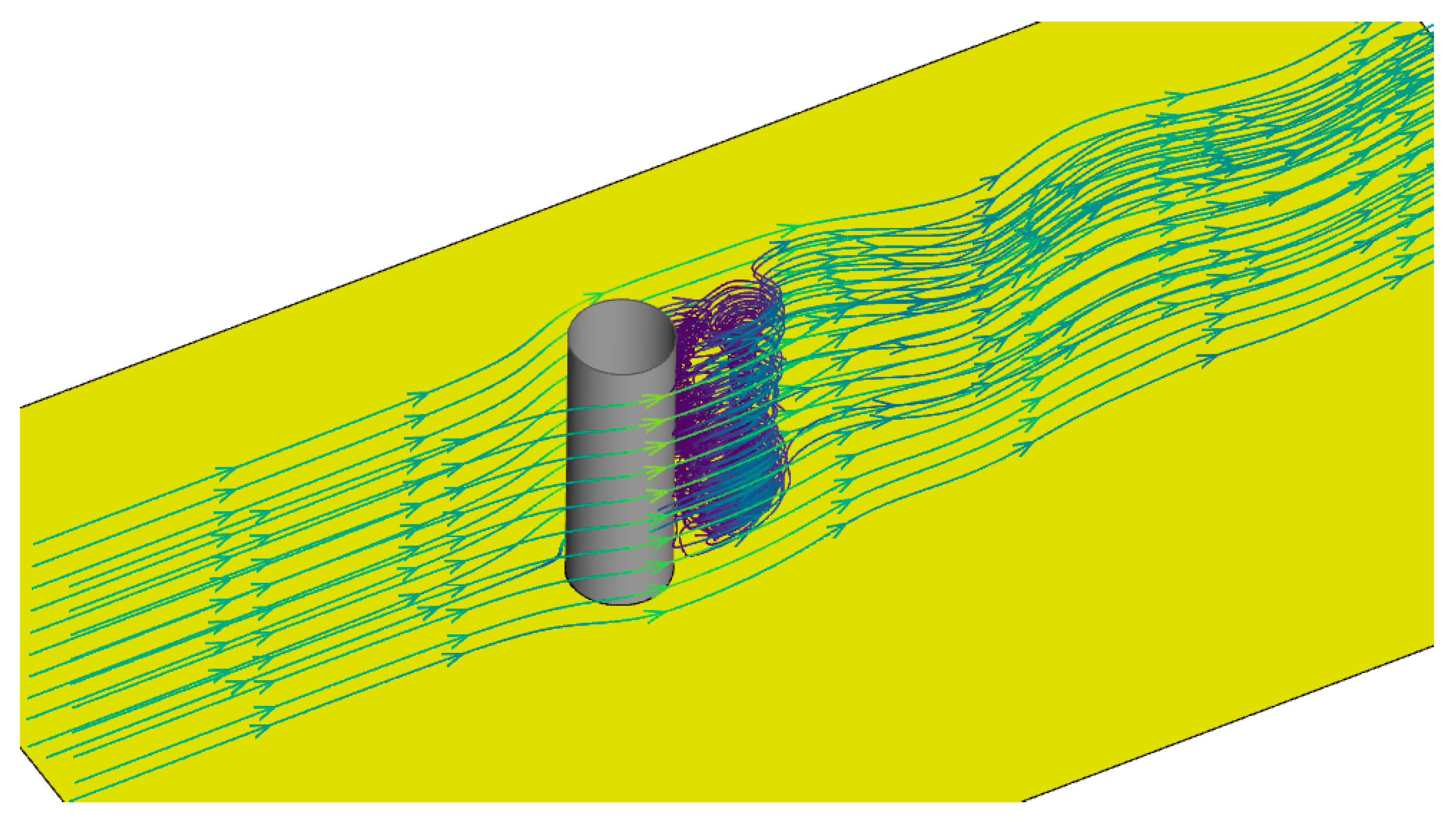
From the experimental results [17], it can be observed that although the water flow velocity on both sides of a single cylindrical bridge pier increases after water blocking, the maximum scouring depth of the single cylindrical bridge pier mainly occurs at the leading edge of the pier. This is mainly because the undercurrent and horseshoe vortex system at the front edge of the bridge pier have an impact, suction, and entrainment effect on the sediment at the front edge of the bridge pier, accelerating the development of the scour depth at the front edge of the bridge pier. This indicates that the turbulent characteristics of water flow contribute significantly to the local scour of bridge piers. In CFD simulations of local scour, the strength of vortices can be characterized by turbulent energy. Therefore, in addition to focusing on the development of the inlet velocity profile along the flow direction, the development of turbulence characteristics such as TKE along the flow direction also needs to be taken into account. The self-sustaining characteristics of turbulent boundary conditions given at the inlet play an important role in the refinement simulation of local scour CFD.

Turbulence inherently possesses a dissipative nature. Turbulent motion is accompanied by a loss of mechanical energy. If no other forms of energy are available for replenishment during turbulent motion, the energy of the turbulent motion will gradually decay. Therefore, in CFD simulations of local scour, it is necessary to find a method that can simulate the equilibrium turbulent boundary layer, providing a new approach for studying local scour problems under specified turbulent boundary conditions.

Based on the assumption of local turbulence equilibrium, the generation term of TKE is equal to the dissipation term. We derived a self-sustaining model (SSM), adopting the solution of its partial differential equation as the boundary condition for turbulence. The specific derivation process is as follows:

$$\epsilon ={C_{\mu }}^{1/2}k(z)\cdot {\displaystyle \frac{\partial u}{\partial z}}$$

(6)

$${\displaystyle \frac{\partial \epsilon }{\partial z}}={C_{\mu }}^{1/2}{\displaystyle \frac{\partial k}{\partial z}}{\displaystyle \frac{\partial u}{\partial z}}+{C_{\mu }}^{1/2}k{\displaystyle \frac{{\partial }^{2}u}{\partial z^2}}={\displaystyle \frac{\epsilon }{k}}{\displaystyle \frac{\partial k}{\partial z}}+{\displaystyle \frac{\epsilon }{\partial u/\partial z}}{\displaystyle \frac{{\partial }^{2}u}{\partial z^2}}$$

(7)

The expression of the velocity profile is assumed as the logarithmic distribution:

$$u={\displaystyle \frac{u_{*}}{K}}\ln ({\displaystyle \frac{z+z_0}{z_0}})$$

(8)

where $z_0$ is the roughness length. $K$ is the constant of Von Karman, usually taken as 0.41. $u_{*}$ is friction velocity. Substituting Equations (6)–(8) into Equations (3) and (4) yields the following:

$${\displaystyle \frac{C_{\mu }}{{\sigma }_k}}{\displaystyle \frac{\partial }{\partial z}}\left({\displaystyle \frac{k^2}{\epsilon }}{\displaystyle \frac{\partial k}{\partial z}}\right)=0$$

(9)

$${\left({\displaystyle \frac{\partial k}{\partial z}}\right)}^2+k{\displaystyle \frac{{\partial }^{2}k}{\partial z^2}}-{\displaystyle \frac{2k}{z}}{\displaystyle \frac{\partial k}{\partial z}}+{\displaystyle \frac{\left(C_{1\epsilon }-C_{2\epsilon }\right){\sigma }_{\epsilon }}{K^2}}{u_{\ast }}^2{\displaystyle \frac{k}{z^2}}+{\displaystyle \frac{k^2}{z^2}}=0$$

(10)

The solution expressions of the combining Equations (8)–(10) are given in Figure 1. Here, the determination of parameters B₁ and B₂ is based on the least squares nonlinear fitting method and flume test data. The detailed process can be found in Yu et al. [31].

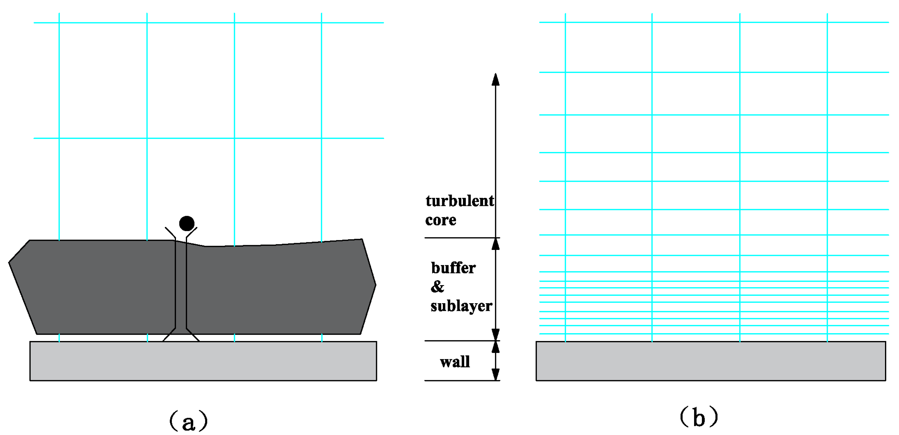
2.4. Near-Wall Treatment Methods

The treatment of near-wall regions typically involves two methods. The wall function method (refer to Figure 2a) employs a semi-empirical formula to address the viscosity-affected zone between the wall surface and the fully turbulent region. However, the internal area influenced by viscosity, encompassing the viscous sublayer and buffer layer, remains unresolved. In another near-wall model approach (see Figure 2b), the viscosity-affected region is solved using a fine mesh [17].

The semi-empirical wall function is utilized to address the incompletely developed turbulence in the viscous sublayer. Typically, the semi-empirical formula for the wall function follows the logarithmic law, as depicted in Equation (11) below:

$$u^{+}={\displaystyle \frac{u}{u_{*}}}={\displaystyle \frac{1}{K}}\ln E{y}^{+}$$

(11)

where $u^{+}$ is the non-dimensional velocity. $u_{*}=\sqrt{{\tau }_{\omega }/\rho }$ is the friction velocity. ${\tau }_w$ is the wall shear stress. $y^{+}={\displaystyle \frac{u_{*}\cdot y_b}{\nu }}$ is the dimensionless length, 30 < $y^{+}$ < 60 [31]. $y_b$ is the distance to the wall. $v$ is the kinematic viscosity. $E$ is the roughness parameter, usually taken as 9.0. The wall shear stress yields the following:

$${\tau }_{\omega }=\left\{\begin{array}{c}k\rho C_{\mu }^{1/4}{K}^{1/2}u/\ln \left(E{y}^{+}\right)\\ \rho \nu \end{array}\right. \begin{array}{c}{y}^{+}>11.225\\ y^{+}<11.225\end{array}$$

(12)

2.5. Sediment Transport Model

The formula for calculating the critical shear stress (${\tau }_{b,cr}$) on a flat riverbed is as follows [32]:

$${\tau }_{b,cr}=\rho g\left(s-1\right)d_{50}{\theta }_{cr}$$

(13)

where $d_{50}$ is the median particle size of sediment. $\mathrm{s}={\rho }_s/\rho$ is the relative density.$g$ is gravitational acceleration. ${\rho }_s$ is sediment density. ${\theta }_{cr}$ is the critical Shields number. The value of ${\theta }_{cr}$ depends on the value of $D_{*}$, and the specific calculation formula refers to Equation (14), in which $D_{*}=d_{50}{[(s-1)g/v^2]}^{1/3}$ [13].

$${\theta }_{cr}=\left\{\begin{array}{c}0.24D_{*}^{-1},D_{*}\le 4\\ 0.14D_{*}^{-0.64},4<D_{*}\le 10\\ 0.04D_{*}^{-0.1},10<D_{*}\le 20\\ 0.13D_{*}^{0.29},20<D_{*}\le 150\\ 0.055,D_{*}>150\end{array}\right.$$

(14)

The terrain of natural riverbeds is not flat. Gravity exerts an influence on both the transport process of sediment and the state of the sediment itself. As shown in Figure 3, the shear stress of a flat riverbed is substituted by equivalent shear stress [33], which is obtained by analyzing the combined force of water resistance and gravity [13].

$${\tau }_{sce}={\tau }_{b,cr}\cos \gamma$$

(15)

$${\tau }_{be}={\tau }_b\sqrt{{\displaystyle \frac{{\left({\tau }_{b,cr}/{\tau }_b\right)}^2{\sin }^2\gamma /{\tan }^2\phi +1-2\left({\tau }_{b,cr}/{\tau }_b\right)\cos {\omega }_z}{\tan \phi }}}$$

(16)

Here, ${\tau }_{sce}$ is the equivalent critical shear stress. ${\tau }_{be}$ is the equivalent shear stress. $\phi$ is the angle of sediment repose. γ is the angle between the $z$ directions and the normal direction on riverbed. ${\tau }_b$ is the shear stress of the riverbed. ${\omega }_z$ is the direction cosine in the $z$ direction.

The excess shear stress T is given as shown in Equation (17).

$$T=\left({\tau }_{be}-{\tau }_{sce}\right)/{\tau }_{sce}$$

(17)

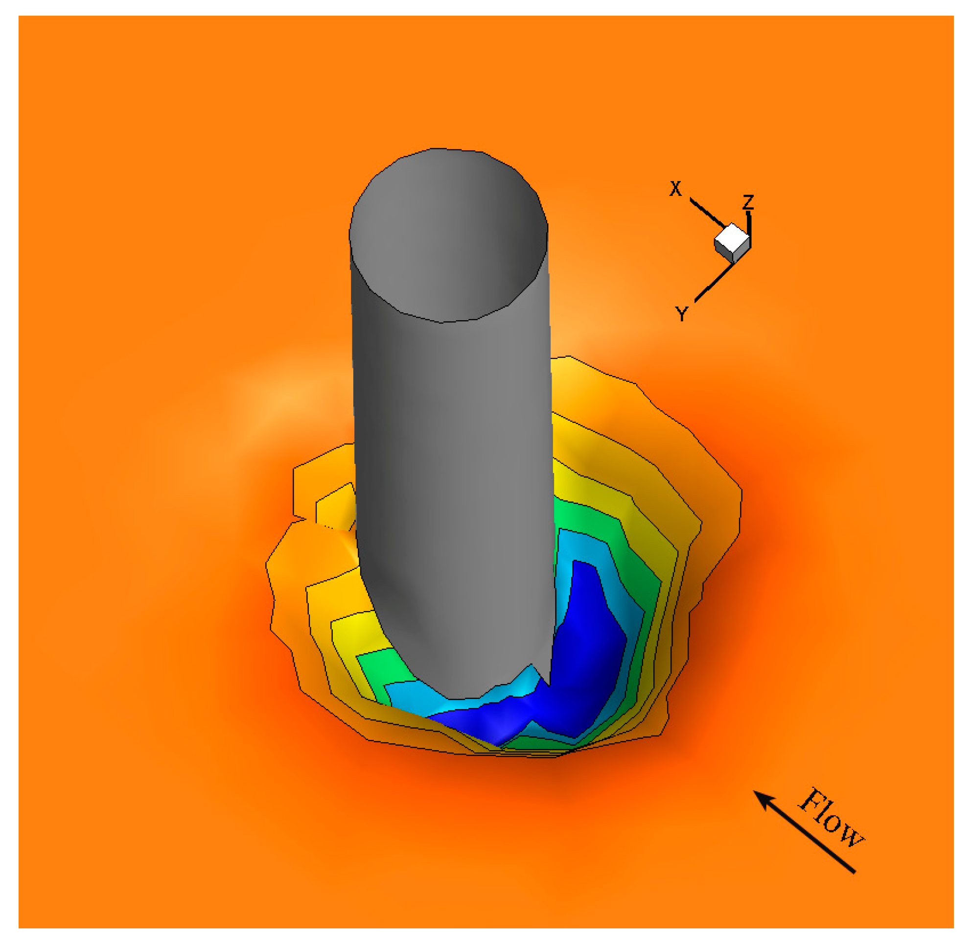
The observation results from numerous local scour flume tests on single cylindrical piers reveal that the maximum scour depth occurs at the leading edge of the pier [9,11]. In this area, the scour depth is significantly influenced not only by the sediment-carrying effect of the approaching water flow but also by the subsurface flow and horseshoe vortex system. To accurately reflect the contribution of turbulent flow characteristics in this region to scouring and to simulate the true shape of the scour pit, we intend to extract the vertical component of water depth in front of the bridge pier and the average shear stress surrounding the pier to adjust the excess shear stress value.

$$T={\displaystyle \frac{\left({\tau }_{be}-{\tau }_{sce}\right)}{{\tau }_{sce}}}+{\displaystyle \frac{C_s\stackrel{\wedge }{{\tau }_{*}}\frac{w}{w_{\max }}}{{{\tau }_{*}}_{cr}}}$$

(18)

Here, $C_s=3.0$ is the empirical constant. $\stackrel{\wedge }{{\tau }_{*}}$ is the average riverbed shear stress around the bridge foundation. $w$ is the average vertical velocity component near the riverbed area at the front edge of the bridge foundation. $w_{\max }$ is the infinite norm of the vertical velocity component at the leading edge of the bridge foundation.

The formula for sediment transport rate is as follows:

$$q_b=0.053\sqrt{\left(s-1\right)g}{d}_{50}^{1.5}{T}^{2.1}{D}_{*}^{-0.3}$$

(19)

The sediment transport rate $q_b$ is decomposed into the streamwise sediment transport rate $q_{bx}$ and cross-flow sediment transport rate $q_{by}$, respectively.

$$q_{bx}={\displaystyle \frac{q_b\left({\tau }_b\cos {\omega }_x+{\tau }_{b,cr}\cos \xi \cos \gamma /\tan \phi \right)}{{\tau }_{be}\cos \alpha }}$$

(20)

$$q_{by}={\displaystyle \frac{q_b\left({\tau }_b\cos {\omega }_y+{\tau }_{b,cr}\cos \delta \cos \gamma /\tan \phi \right)}{{\tau }_{be}\cos \beta }}$$

(21)

Here, $\xi$, $\delta$ are the angles between the $x, y$ directions and the normal direction of riverbed, respectively. $\alpha$, $\beta$ are the stream-wise and cross-flow riverbed slope. ${\omega }_x$, ${\omega }_y$ are the direction cosine in the $x$ and $y$ directions.

The expression for the change in riverbed topography over time is shown in Equation (22).

$${\displaystyle \frac{\partial z}{\partial t}}=-{\displaystyle \frac{1}{1-n}}\left({\displaystyle \frac{\partial q_{bx}}{\partial x}}+{\displaystyle \frac{\partial q_{by}}{\partial y}}\right)$$

(22)

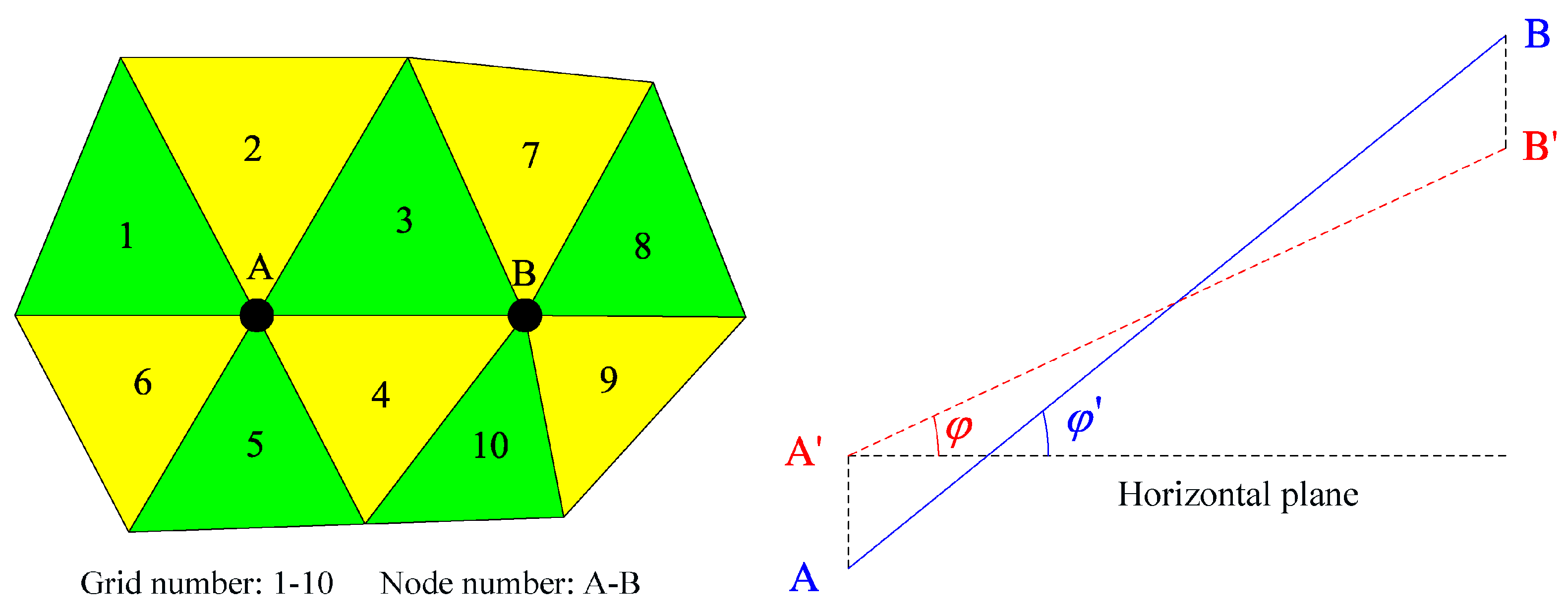
2.6. Sediment-Sliding Model

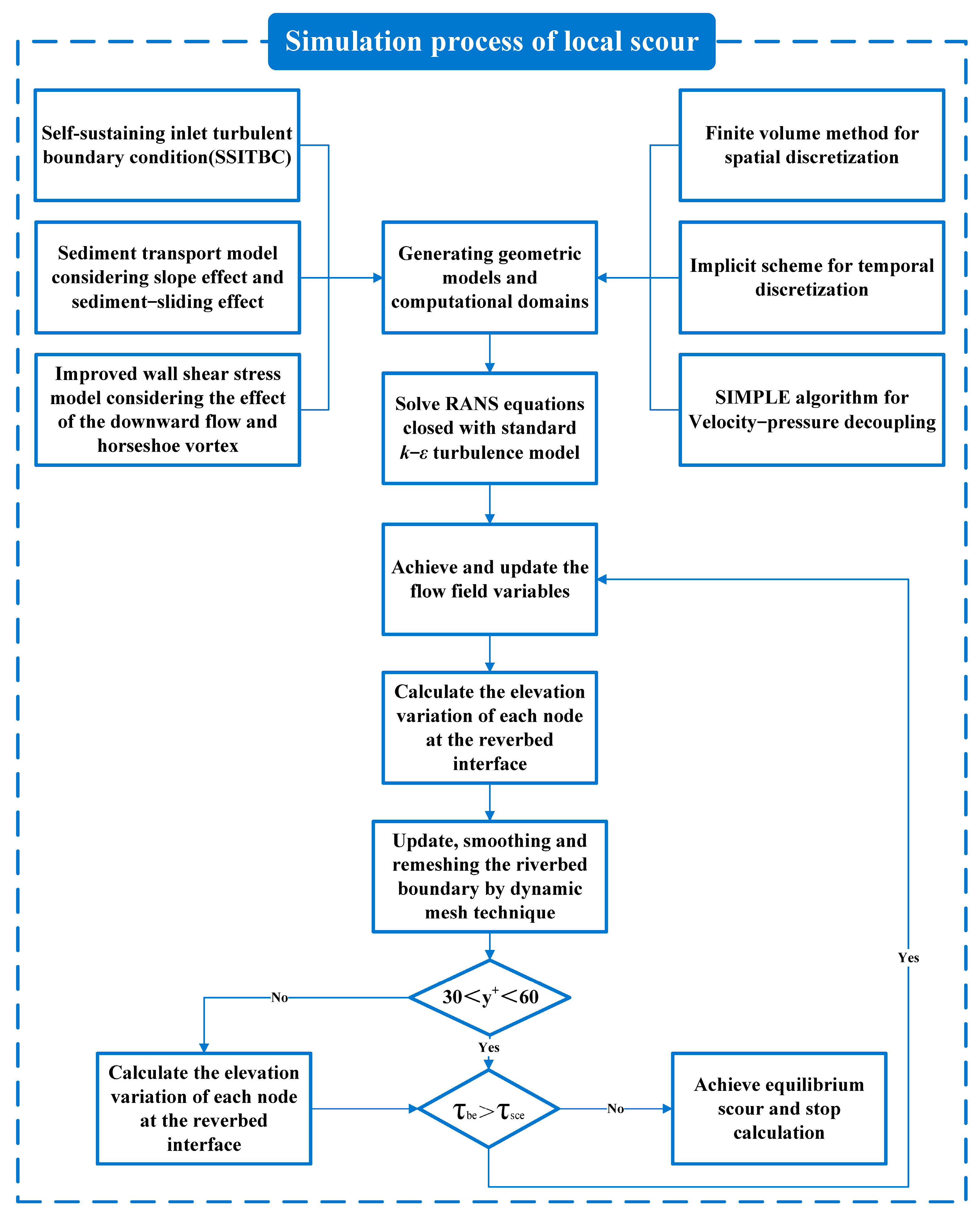
During the process of scouring, the approaching flow is carrying and entraining the sediment particles onto the slopes of scour pit. When the angle between the sand grains is slightly higher than the angle of repose of the sediment, the sediment particles will slide down to reach a new equilibrium and finally stop at an angle slightly lower than the angle of repose of the sediment. To accurately represent this process and reasonably simulate the actual sediment scour and deposition process as well as the shape of the scour pit, a sediment-sliding model is considered for characterization. In the numerical implementation process, the sediment transport rate is calculated by scanning all grid nodes along the riverbed boundary, extracting the shear stress on the riverbed wall, and further calculating the elevation changes of the riverbed nodes. The specific calculation process is shown in Figure 4, while Figure 5 illustrates a working mechanism of the sediment-sliding model. When the inclination angle of the connection between adjacent grid nodes scanning the global grid is greater than the angle of repose of the sediment, the positions of the nodes at both ends of the connection will be dynamically adjusted to be equal to the angle of repose of the sediment to maintain a balanced state at the angle of repose of the sediment.

$$\left(z_B-\Delta z_B\right)-\left(z_A+\Delta z_A\right)=\tan \phi \sqrt{{\left(x_A-x_B\right)}^2+{\left(y_A-y_B\right)}^2}$$

(23)

$$\left({\mathrm{A}}_1+{\mathrm{A}}_2+{\mathrm{A}}_3+{\mathrm{A}}_4+{\mathrm{A}}_5+{\mathrm{A}}_6\right)\mathsf{\Delta }{z}_A=\left({\mathrm{A}}_3+{\mathrm{A}}_4+{\mathrm{A}}_7+{\mathrm{A}}_8+{\mathrm{A}}_9+{\mathrm{A}}_{10}\right)\mathsf{\Delta }{z}_B$$

(24)

Here, $x_A,y_A,z_A$ and $x_B,y_B,z_B$ are the coordinates of Points A and B, respectively. $\Delta z_A$, $\Delta z_B$ are the variations in Points A and B, respectively. A₁ … A₁₀ is the area of the adjacent surface between A and B.

3. Numerical Implementations

3.1. Physical Flume Experiment

The validation of the numerical model adopts the classic Melville flume experiment [9]. The flume in the model has a length of 19 m and a width of 45.6 cm, while the water depth is 15 cm. The longitudinal slope of the riverbed is 1/10,000. The pier has a diameter D of 5.08 cm. Figure 6 provides the layout diagram of the flume experiment. The sediment in the model has a median diameter (d₅₀) of 0.385 mm, with a repose angle of 32°. The mean velocity is 0.25 m/s. The Reynolds number for selecting the pier diameter as the characteristic length is $R{e}_D=12677$. The Froude number F_r = 0.13. Figure 7 presents the undisturbed velocity and TKE profile before the pier. The fitting parameters of the self-sustaining inlet turbulent boundary conditions are given in

Table 2. Fitting parameters of the SSITBC.

$\mathit{u}*$	${\mathit{z}}_0$	${\mathit{B}}_1$	${\mathit{B}}_2$	${\mathit{C}}_{\mathit{\mu }}$
0.0118	0.000013	−0.14	1.69	0.015

.

3.2. Numerical Flume Experiment

The calculation domain size and boundary conditions for local scour CFD simulation in this article are set as shown in Figure 8. The total length of the computational domain is 18D; the length from the entrance to the model position is 6D; and the length from the model position to the exit is 12D [32]. The width of the calculation domain is consistent with the width of the physical water flume, which is 45.6cm. The height of the computational domain is consistent with the water depth of the physical water flume experiment, which is 15cm. We calculate the turbulent boundary conditions at the entrance of the computational domain, including the velocity and TKE profiles. The given profile shape is shown in Figure 7. It should be pointed out that before conducting CFD simulations of local scour spatiotemporal evolution, it is necessary to perform self-sustaining characteristic tests on the turbulent boundary conditions given at the inlet in the empty computational domain flow field. The exit of the domain is set as the outflow. Both sides of the computational domain, the bottom riverbed boundary, and the pier wall boundary are set as rough wall boundaries. For the top boundary of the calculation domain, according to the literature [26], When H/D > 2.5, the impact of free liquid surface scouring on the riverbed bottom can be ignored. Based on the rigid-cover hypothesis, the top boundary is set as a symmetrical boundary, which will help reduce the number of grids used to capture free liquid surface fluctuations.

Figure 9 shows the spatial discretization of the computational domain using an unstructured tetrahedral mesh. Unstructured grids have strong advantages over structured grids in fitting irregular terrain and improving the problem of large deformation and grid distortion of riverbed surfaces during local scour evolution. At the same time, density box tools are used to locally densify the mesh in areas with significant changes in flow gradients such as bridge piers and riverbed boundaries in order to better capture flow characteristics.

The quality of the grid directly determines the accuracy of the calculation results. The discrimination of grid quality in local scour CFD calculation mainly includes two aspects. One is to choose different turbulence models to meet their different requirements for y⁺ values, and the determination of the height of the first layer grid has a significant impact on the estimation of y⁺ values. Before conducting local scour CFD simulations, it is necessary to conduct grid independence tests to minimize the impact of the grid on the numerical results. The detailed parameters of the grid in different cases are given in

Table 3. Grid independence examination.

Case Number	$\mathbf{Minimum} \mathbf{Grid} \mathbf{Size}$(lmin/D)	$\mathbf{Maximum} \mathbf{Grid} \mathbf{Size}$(lmax/D)	Grid Growth Factor	Grid Quantity	Wall Shear Stress
1	0.04	0.31	1.13	≈1.2 × 105	0.58
2	0.04	0.31	1.10	≈2.4 × 105	0.67
3	0.04	0.31	1.07	≈4.9 × 105	0.68
4	0.04	0.31	1.03	≈1.5 × 106	0.67

. l_max represents the maximum grid size. l_min represents the minimum grid size. The wall shear stress around the pier serves as a criterion parameter for a grid independence check. The final chosen mesh parameters are given in

Table 4. Chosen mesh parameters.

$\mathbf{Minimum} \mathbf{Mesh} \mathbf{Size}$(lmin/D)	$\mathbf{Maximum} \mathbf{Mesh} \mathbf{Size}$(lmax/D)	Mesh Growth Factor	Mesh Quantity
0.04	0.31	1.10	243,369

. According to the approaches described by Yu et al. [31], the optimized parameters of the standard $k-\epsilon$ turbulence model are given in

Table 5. Optimized standard k − ε turbulence model parameters.

${\mathit{C}}_{\mathsf{\mu }}$	${\mathit{\sigma }}_{\mathit{k}}$	${\mathit{\sigma }}_{\mathit{z}}$	${\mathit{C}}_{1\mathit{\epsilon }}$	${\mathit{C}}_{2\mathit{\epsilon }}$
0.015	2.04	2.86	1.44	1.92

, which is used for subsequent CFD simulation. The main process of CFD simulation for local scour of bridge foundation in this article is shown in Figure 10. The numerical strategies in the CFD simulation of local scour are given in Figure 11.

4. Results and Discussion

4.1. Self-Sustaining Characteristic Examination

Figure 12 shows a comparison of the results of the velocity and TKE profiles at different positions within the computational domain when using the averaged velocity method, the traditional method, and the self-sustaining method. It can be seen that for the average velocity method, the average velocity and TKE profiles obtained at L/3 significantly deviate from the target profiles. The velocity profile obtained using the traditional method exhibits a decaying state in the area where z > 0.05 m, while it shows a slight increase in the area where z < 0.5 m. There is an obvious attenuation in the TKE profile. However, at L/3, the TKE shows an increase in the part where z > 0.04. These changes in the target flow conditions may lead to significant alterations in the local scour patterns. By adopting the self-sustaining method proposed by the author, an equilibrium turbulent boundary layer can be simulated, and the velocity and TKE profiles specified at the inlet display good self-sustaining characteristics along the flow direction.

4.2. Initial Scouring

The instantaneous bed wall shear stress in the initial scouring is shown in Figure 13. At the initial stage, the maximum shear stress occurs in the area between both sides of the bridge pier, with a value of 0.67 Pa. This area is also the area around the bridge pier where local scour first occurs. These observed phenomena are consistent with that described during the flume experiment [9].

Figure 14 shows the streamwise velocity components. Upstream of the bridge pier, the velocity profile within the boundary layer exhibits a distinct exponential or logarithmic profile. When approaching the area affected by the bridge pier, the water flow velocity gradually decreases due to the obstruction of the bridge pier. Downstream of the bridge pier, the velocity after the flow has not yet developed into a new exponential or logarithmic velocity profile due to the disturbance of the bridge pier. A vacuum zone was created near the wake region of the bridge pier because of the presence of a reverse pressure gradient.

Figure 15 shows the velocity components along the direction of the water depth. Affected by the obstruction of the bridge pier, the separation flow occurs simultaneously upwards and downwards along the bridge pier. The upward flow generates backwater. The downward flow may interweave with the approaching water flow to form a horseshoe vortex. Due to the assumption of rigid cover in the simulation of this paper, the free surface was not simulated, and the phenomenon of backwater was not observed in the figure. The area where the downward flow occurs is obvious in the figure. The vertical velocity component in this area is also the data that need to be monitored for correcting the excess shear stress in the riverbed mentioned above.

Figure 16 shows the streamwise velocity vector. The red box at the leading edge of the bridge pier indicates the downward flow caused by the blocking of the bridge pier. The red circle in the wake area of the bridge pier indicates the reverse flow region formed by the backflow at the rear edge of the bridge pier, where wake vortices of varying sizes may form. The vortex formed near the riverbed wall may have a relatively small scale due to its constraints on the riverbed wall.

Figure 17 shows the three-dimensional streamline around the pier. The rotating flow of streamlines can be clearly seen in the wake area of the bridge pier, indicating the presence of wake vortex flow characteristics in this area. Figure 18 shows the vorticity contour calculated using the Q criterion. There are obvious vertical vortices and alternating shedding of vorticity in the wake area of the bridge pier. There is a weak horseshoe vortex system in front of the pier. Compared to the case of using LES calculation [34], the vorticity of the horseshoe vortex system in front of the pier is smaller. This further illustrates the limitations of using the k − ε turbulence model to estimate the horseshoe vortex system in front of the pier.

4.3. Medium Scouring Phase

Figure 19 shows a comparison between the simulation results and experimental results of the morphology of the scour pit during the intermediate scouring phase. As can be seen, the maximum scouring depth at this time is about 4 cm, and the shape of the scouring pit is consistent. The simulated maximum scouring depth position is consistent with the experimental results, all located at the front edge of the bridge pier. This indicates that the method proposed in this article can reasonably reflect the contribution of the downward flow and horseshoe vortex in front of the pier to the scouring depth of the bridge pier’s leading edge, and we obtain a maximum scouring depth and scouring pit shape that are consistent with the experimental results. We improved and optimized the situation where the maximum scour pit occurs on both sides of the bridge pier when using traditional methods for numerical simulation of local scour.

Figure 20 and Figure 21 show the riverbed elevations in both the streamwise and transverse directions during scouring, respectively. As can be seen, the maximum local scouring depth of the bridge pier at this time is 4 cm. The development range of the scouring pit at the front edge of the bridge pier is approximately 1.2D, and the development range of the scouring pit on both sides of the bridge pier is about 1.1D. The scope and shape of the scouring pit on both sides of the bridge pier is based on the symmetry of the axial plane in the clockwise direction. The slope angle of the scouring pit wall is approximately 31°, which is close to the sediment rest angle of 32° in the experimental results, indicating that the sediment-sliding model introduced in this article can reasonably reflect the sediment-sliding process in local scour. In the wake area of the rear edge of the bridge pier, influenced by the wake vortex, the development range of the scour pit is approximately 0.8D. There is a small area near the rear edge of the bridge pier where there is no significant scouring, and the scour depth is significantly smaller than that in front of the pier and on both sides.

4.4. Equilibrium Scour Phase

Figure 22 shows a comparison of the scour pit after achieving equilibrium scour. The maximum scouring depth simulated using traditional methods occurs on both sides of the bridge pier, while the maximum scouring depth simulated using the numerical method considering the influence of turbulence characteristics in this paper is consistent with the experimental results and occurs at the front edge of the bridge pier. This indicates that the SSM and the improved wall shear stress model considering the effects of undercurrent and horseshoe vortices proposed in this article can reasonably reflect the contribution of turbulent characteristics to the scour in front of bridge piers. In addition, when achieving equilibrium scour, the maximum scouring depth of the riverbed is about 6 cm, and the location where the maximum scouring depth occurs is still at the front edge of the bridge pier. The simulation results are consistent with the experimental results. Compared with the contour map of the scour pit in Figure 19, in addition to the further development of the maximum scour depth of the scour pit, the development range of the scour pit has increased, and the scope of the scour pit on both sides of the bridge pier has extended from 1.1D to 1.3D. The scouring pit in front of the bridge pier extends from 1.2D to 1.6D, and the trailing edge of the bridge pier extends from 0.8D to 1D. In addition, the area where there is no significant scour at the rear edge of the bridge pier has also developed compared to before. Figure 23 shows the three-dimensional scour pit morphology after achieving equilibrium scour. The shape of the scouring pit around the bridge pier can be observed in the figure, with the maximum scouring depth occurring at the leading edge of the bridge pier.

4.5. Variations in Scour Depth over Time

Figure 24 and Figure 25 show the development process of scour hole morphology over time in the streamwise and transverse directions, respectively. In the first 30 min of scour development, the rate of scour depth development is relatively fast, and the depth of the scour pit develops significantly, especially at the front edge and sides of the bridge piers. In the last 30 min of scour development, the scour rate gradually slows down until equilibrium scour is reached. In fact, the time in numerical simulations cannot be completely matched with that in real physical flume experiments. This may be due to the fact that both the turbulence model and the sediment model used in the numerical simulation of local scour are semi-empirical and semi-theoretical models. Consequently, further optimization is required in predicting the time development process of the scour depth. However, the variation law of the scour development rate demonstrated in the numerical simulation is similar to that presented in the physical flume experiment. Moreover, on the spatial scale after the equilibrium scour, the maximum scour depth and the morphology of the scour pit can be compared. This is because the change in the riverbed elevation depends on the sediment transport rate in the sediment model. The sediment transport rate is determined by the excess shear stress of the riverbed, and the excess shear stress is mainly affected by the riverbed topography, roughness height, flow velocity, and turbulent conditions.

In the upstream direction, the scour development speed at the leading edge of the bridge pier is much greater than that at the trailing edge. The maximum scour depth and slope shape of the scour pit after balancing the scouring at the leading edge are consistent with the experimental results. However, the development depth of the scour hole at the rear edge of the bridge pier is far less than the experiment results, only reaching 50% of the test results. In the transverse flow direction, the development of the scour pit on both sides of the bridge pier is synchronous and symmetrical with time, which is consistent with the experimental observation results. After reaching equilibrium scour, the shape of the scour pit on both sides of the bridge pier is consistent with the experimental results, with a maximum scour depth of about 0.7D, which is 10% smaller than the experimental results. This indicates that the method proposed in this article can effectively solve the problem of insufficient estimation of local scour depth in the area by the downward-flow and horseshoe vortex system in front of the pier.

5. Conclusions

This article conducts a numerical study on the local scour of a three-dimensional single-cylinder pier based on a self-sustaining model and an improved wall shear stress model. The main conclusions are as follows:

The self-sustaining model (SSM) proposed can quickly simulate the equilibrium turbulent boundary layer at the riverbed wall, optimize and enhance the self-sustaining characteristics of the specified velocity and TKE profile at the inlet, and ensure the consistency of the turbulence characteristics in the model area with the target value. In addition, when studying structures such as underwater oil pipelines, turbulent pulsation characteristics are particularly important, especially when it comes to vortex-induced vibration problems in flexible pipelines and vortex sand-carrying problems caused by local scour around pipelines. Therefore, self-sustaining models can provide new ideas and methods for the fine simulation of specified flow conditions in the CFD simulation of these issues.

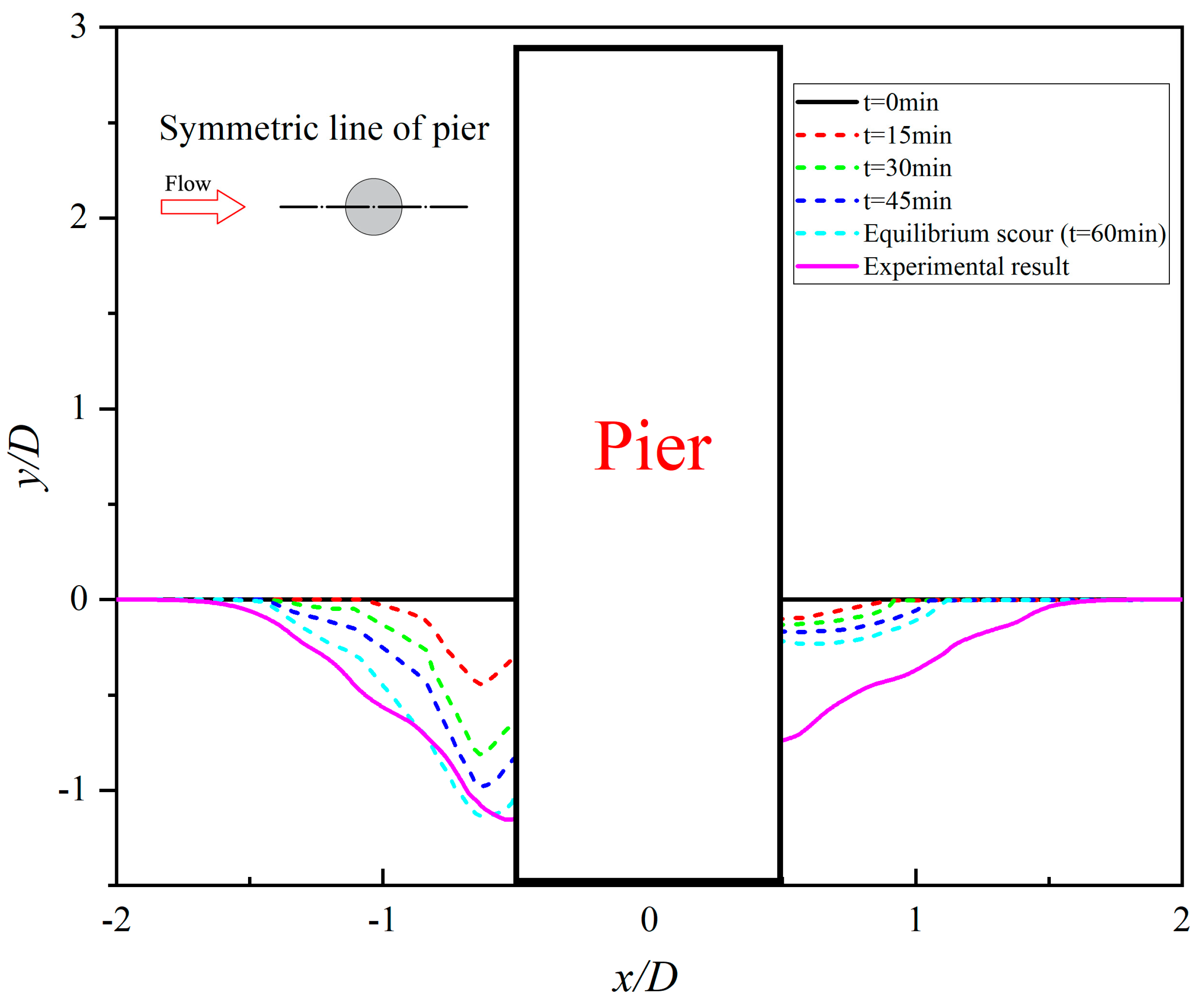
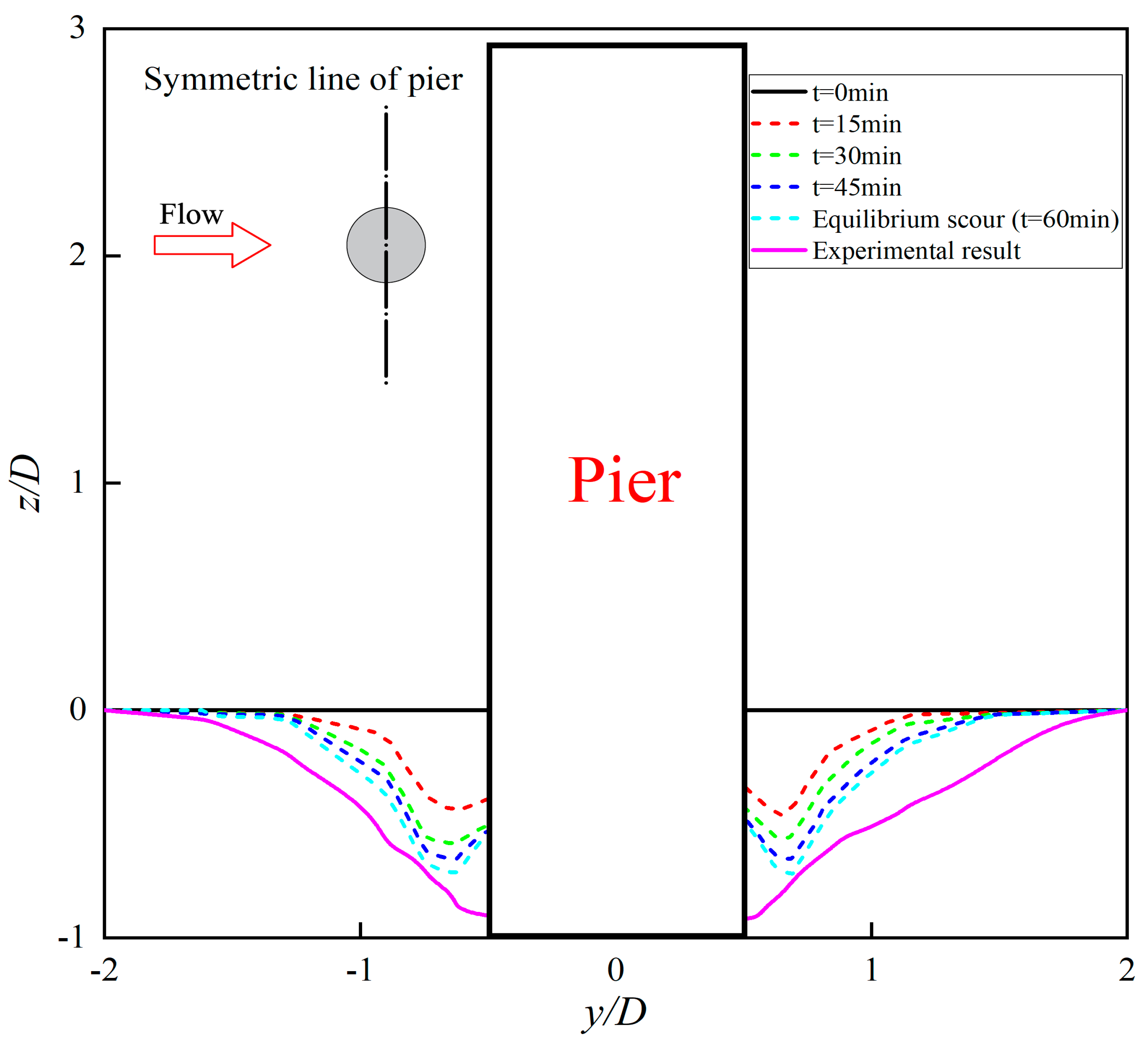
The proposed improved wall shear stress model can effectively solve the problem of insufficient estimation of local scour depth in the area by the downward flow and horseshoe vortex system in front of the pier. The maximum scour depth obtained from the simulation is consistent with the experiment in terms of both size and location. However, there are still some shortcomings in the estimation of scour and sedimentation in the wake area of bridge piers. In the future, the accuracy of the model’s scour and deposition estimation in the wake region will be further optimized and improved. Furthermore, this provides a reference and basis for the detailed simulation of scour on structures such as bridge foundations, offshore wind turbines, and submarine pipelines in the future.

References

1. Bharadwaj, M.R.; Gupta, L.K.; Pandey, M.; Valyrakis, M. Countermeasures for local scour around the bridge pier: A review. Acta Geophys. 2024. [Google Scholar] [CrossRef]
2. Yu, P.; Chen, J.C.; Zhou, J.L.; Li, J.; Yu, L. Experimental investigation of local scour around complex bridge pier of sea-crossing bridge under tidal currents. Ocean Eng. 2023, 290, 116374. [Google Scholar] [CrossRef]
3. Tafarojnoruz, A.; Gaudio, R.; Calomino, F. Bridge pier scour mitigation under steady and unsteady flow conditions. Acta Geophys. 2012, 60, 1076–1097. [Google Scholar] [CrossRef]
4. Gaudio, R.; Tafarojnoruz, A.; Calomino, F. Combined flow-altering countermeasures against bridge pier scour. J. Hydraul. 2012, 50, 35–43. [Google Scholar] [CrossRef]
5. Ferraro, D.; Tafarojnoruz, A.; Gaudio, R.; Cardoso, A.H. Effects of Pile Cap Thickness on the Maximum Scour Depth at a Complex Pier. J. Hydraul. 2013, 139, 482–491. [Google Scholar] [CrossRef]
6. Pandey, M.; Valyrakis, M.; Qi, M.L.; Sharma, A.; Lodhi, A.S. Experimental assessment and prediction of temporal scour depth around a spur dike. Int. J. Sediment. Res. 2021, 36, 17–28. [Google Scholar] [CrossRef]
7. Liu, D.; Alobaidi, K.; Valyrakis, M. The assessment of an acoustic Doppler velocimetry profiler from a user’s perspective. Acta Geophys. 2022, 70, 2297–2310. [Google Scholar] [CrossRef]
8. Wu, P.; Ram, B.; Sui, J. Local scour around bridge piers under ice-covered conditions. J. Hydraul. Eng. 2016, 142, 04015038. [Google Scholar] [CrossRef]
9. Melville, B. Local Scour at Bridge Sites; The University of Auckland: Auckland, New Zealand, 1975. [Google Scholar]
10. Liang, F.; Wang, C.; Huang, M.; Wang, Y. Experimental observations and evaluations of formulae for local scour at pile groups in steady currents. Mar. Georesour. Geotechnol. 2016, 35, 245–255. [Google Scholar] [CrossRef]
11. Nielsen, A.; Liu, X.; Sumer, B.; Fredsøe, J. Flow and bed shear stresses in scour protections around a pile in a current. Coast. Eng. 2013, 72, 20–38. [Google Scholar] [CrossRef]
12. Otoo, E.; Asumadu, R.; Boadi, G.K.; Zhang, J.S.; Boadu, S.; Mattah, P. Numerical investigation of scour around monopile foundation of offshore wind farm. Discov. Appl. Sci. 2024, 6, 11. [Google Scholar] [CrossRef]
13. Chen, X.; Ma, J.; Dey, S. Sediment transport on arbitrary slopes: Simplified model. J. Hydraul. Eng. 2010, 136, 311–317. [Google Scholar] [CrossRef]
14. Salaheldin, T.; Imran, J.; Chaudhry, H. Numerical modeling of three-dimensional flow field around circular piers. J. Hydraul. Eng. 2004, 130, 91–100. [Google Scholar] [CrossRef]
15. Ahmad, N.; Kamath, A.; Bihs, H. 3D numerical modelling of scour around a jacket structure with dynamic free surface capturing. Ocean Eng. 2020, 200, 107104. [Google Scholar] [CrossRef]
16. Olsen, N.; Melaaen, M. Three-dimensional calculation of scour around cylinders. J. Hydraul. Eng. 1993, 119, 1048–1054. [Google Scholar] [CrossRef]
17. Roulund, A.; Sumer, B.; Fredsøe, J.; Michelsen, J. Numerical and experimental investigation of flow and scour around a circular pile. J. Fluid. Mech. 2005, 534, 351–401. [Google Scholar] [CrossRef]
18. Wei, K.; Jiang, M.; Hong, J. Numerical simulation of mechanical characteristics of round ended pier impacted by breaking wave. Ocean Eng. 2021, 39, 111–118. [Google Scholar] [CrossRef]
19. Liu, Q.; Wang, Z.; Zhang, N.; Zhao, H.; Liu, L.; Huang, K.; Chen, X. Local Scour Mechanism of Offshore Wind Power Pile Foundation Based on CFD-DEM. J. Mar. Sci. Eng. 2022, 10, 1724. [Google Scholar] [CrossRef]
20. Zheng, Z.Y.; Hu, Z.; Xie, X.G.; Huang, W. Local scour around the monopile: A microscopic perspective using CFD-DEM. Ocean Eng. 2024, 299, 117318. [Google Scholar] [CrossRef]
21. Kirkil, G.; Constantinescu, G.; Ettema, R. Detached eddy simulation investigation of turbulence at a circular pier with scour hole. J. Hydraul. Eng. 2009, 135, 888–901. [Google Scholar] [CrossRef]
22. Zhang, S.Y.; Li, B.E.; Ma, H.H. Numerical investigation of scour around the monopile using CFD-DEM coupling method. Coast. Eng. 2023, 183, 104334. [Google Scholar] [CrossRef]
23. Nikeghbali, P.; Benjankar, R.; Kheirkhahan, M. Erosion under drawdown flushing with the SPH method. Ocean Eng. 2024, 310, 118743. [Google Scholar] [CrossRef]
24. Khanpour, M.; Zarrati, A.R.; Kolahdoozan, M.; Shakibaeinia, A.; Amirshahi, S.M. Mesh-free SPH modeling of sediment scouring and flushing. Comput. Fluids. 2016, 129, 67–78. [Google Scholar] [CrossRef]
25. Zhang, R.Z.; Xiong, X.; Gao, Y.F. A meshless model for three-dimensional direct numerical simulation of local scour around cylinder bridge foundation. Ocean Eng. 2024, 312, 119220. [Google Scholar] [CrossRef]
26. Yu, P.; Zhu, L. Numerical simulation of local scour around bridge piers using novel inlet turbulent boundary conditions. Ocean Eng. 2020, 218, 108166. [Google Scholar] [CrossRef]
27. Alemi, M.; Pêgo, J.; Maia, R. Numerical investigation of the flow behavior around a single cylinder using large eddy simulation model. Ocean Eng. 2017, 145, 464–478. [Google Scholar] [CrossRef]
28. Jia, Y.F.; Altinakar, M.; Guney, M.S.; Guney, M.S. Three-dimensional numerical simulations of local scouring around bridge piers. J. Hydraul. Res. 2017, 56, 351–366. [Google Scholar] [CrossRef]
29. Xiong, W.; Cai, C.S.; Kong, B.; Kong, X. CFD simulations and analyses for bridge-scour development using a dynamic-mesh updating technique. J. Comput. Civ. Eng. 2014, 30, 04014121. [Google Scholar] [CrossRef]
30. Yu, P.; Liu, J.F.; Yu, L.; Zhu, L.K. Numerical investigation of local scour around tandem piers using proposed self-sustaining inlet turbulent boundary conditions. Ocean Eng. 2023, 274, 113987. [Google Scholar] [CrossRef]
31. Yu, P.; Liu, J.F.; Sun, Z.W. Study on the self-sustaining inlet boundary conditions for numerical simulation on local scour. J. Waterw. Port Coast. Ocean Eng. 2020, 146, 04020027. [Google Scholar] [CrossRef]
32. Sarker, M. Flow measurement around scoured bridge piers using acoustic-doppler velocimeter (ADV). Flow Meas. Instrum. 1998, 9, 217–227. [Google Scholar] [CrossRef]
33. Rijn, L. Sediment transport, Part I: Bed load transport. J. Hydraul. Eng. 1984, 110, 1431–1457. [Google Scholar] [CrossRef]
34. Zhang, H.; Yang, J.M.; Xiao, L.F.; Lu, H.N. Large-eddy simulation of the flow past both finite and infinite circular cylinders at Re = 3900. J. Hydrodyn. B 2015, 27, 195–203. [Google Scholar] [CrossRef]
Figure 1. Novel self-sustaining inlet turbulent boundary conditions (SSITBC).
Jmse 12 02187 g001
Figure 2. Solution method for near-wall region. (a) Wall function approach; (b) near-wall model approach.
Jmse 12 02187 g002
Figure 3. Sketch of the equivalent shear stress.
Jmse 12 02187 g003
Figure 4. Process of the sediment-sliding model.
Jmse 12 02187 g004
Figure 5. Sketch of adjusting the tilt angle of two nodes.
Jmse 12 02187 g005
Figure 6. Layout of flume experiment.
Jmse 12 02187 g006
Figure 7. Fitting results of inlet turbulence conditions: (a) velocity profile; (b) TKE profile.
Jmse 12 02187 g007
Figure 8. Boundary condition setting for numerical flume.
Jmse 12 02187 g008
Figure 9. Unstructured tetrahedral mesh.
Jmse 12 02187 g009
Figure 10. Detailed process of the CFD simulation for local scour.
Jmse 12 02187 g010
Figure 11. Detailed numerical strategies.
Jmse 12 02187 g011
Figure 12. Comparison of calculation results among the averaged velocity method, the traditional method, and the self-sustaining method: (a) the velocity profile using the averaged velocity method; (b) the TKE profile using the averaged velocity method; (c) the velocity profile using the traditional method; (d) the TKE profile using the traditional method; (e) the velocity profile using the self-sustaining method; (f) the TKE profile using the self-sustaining method.
Jmse 12 02187 g012
Figure 13. Instantaneous wall shear stress in the initial scouring (unit: Pa).
Jmse 12 02187 g013
Figure 14. Streamwise velocity component.
Jmse 12 02187 g014
Figure 15. Velocity component based on water depth.
Jmse 12 02187 g015
Figure 16. Streamwise velocity vector.
Jmse 12 02187 g016
Figure 17. Streamline around the pier before scouring.
Jmse 12 02187 g017
Figure 18. Vortical structures revealed by iso-surface of the Q criterion (Q = 0.2).
Jmse 12 02187 g018
Figure 19. Contour of scour pit in medium scouring phase.
Jmse 12 02187 g019
Figure 20. Longitudinal-sectional view of the scour pit.
Jmse 12 02187 g020
Figure 21. Cross-sectional view of the scour pit.
Jmse 12 02187 g021
Figure 22. Comparing the equilibrium scour pit: (a) experimental results by Melville 1975 [9]; (b) simulated results using the proposed approach; (c) simulated results by Yu et al., 2020 [31]; (d) simulated results by Xiong et al., 2014 [29].
Jmse 12 02187 g022
Figure 23. Equilibrium scour pit morphology.
Jmse 12 02187 g023
Figure 24. Evolution of scour pit over time in the streamwise direction.
Jmse 12 02187 g024
Figure 25. Evolution of scour pit over time in the transverse direction.
Jmse 12 02187 g025