
The Path Tracking Control of Unmanned Surface Vehicles Based on an Improved Non-Dominated Sorting Genetic Algorithm II-Based Multi-Objective Nonlinear Model Predictive Control Method


Abstract
1. Introduction
- To enhance the trajectory tracking performance of unmanned surface vessels (USVs), this paper employs a time-varying look-ahead distance, treating it alongside the desired velocity and acceleration as parameters to be calculated within the MPC algorithm;
- Given that the cost function of the MPC algorithm comprises multiple objective terms that may conflict with one another, a single-objective optimization approach could lead to a decline in the performance of other metrics. Therefore, this paper utilizes a multi-objective MPC algorithm, enabling comprehensive consideration of multiple performance indicators through multi-objective optimization, thereby identifying the optimal balance among the various objectives;
- This paper adopts an improved NSGAII algorithm within the multi-objective MPC framework, incorporating an adaptive rotation-based simulated binary crossover operation to enhance diversity and convergence. Additionally, the method of non-dominated sorting has been refined. These improvements help to prevent premature convergence while also reducing computational time.
2. Mathematical Modeling
2.1. Models Used to Simulate the Vessel
2.2. Models Used for Predictions
3. Path Tracking
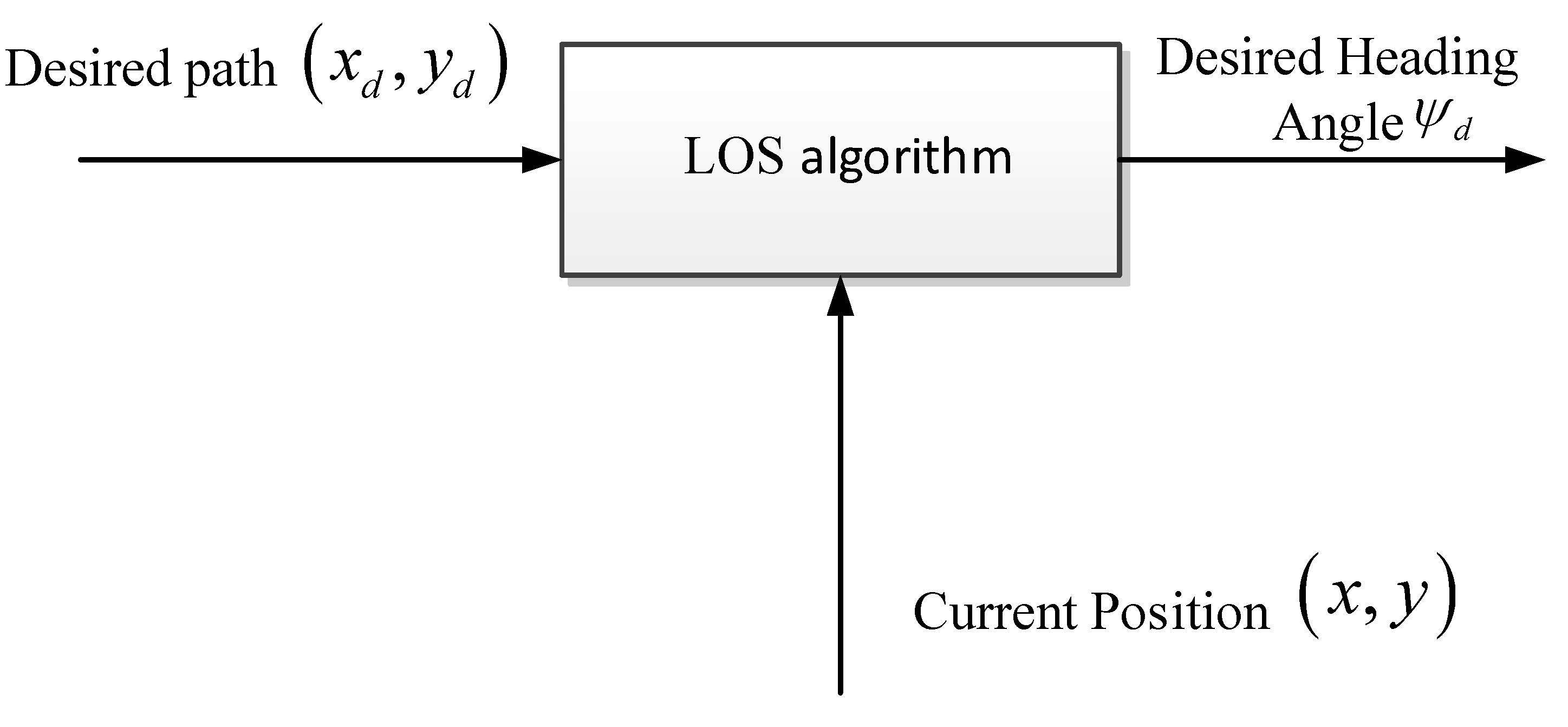
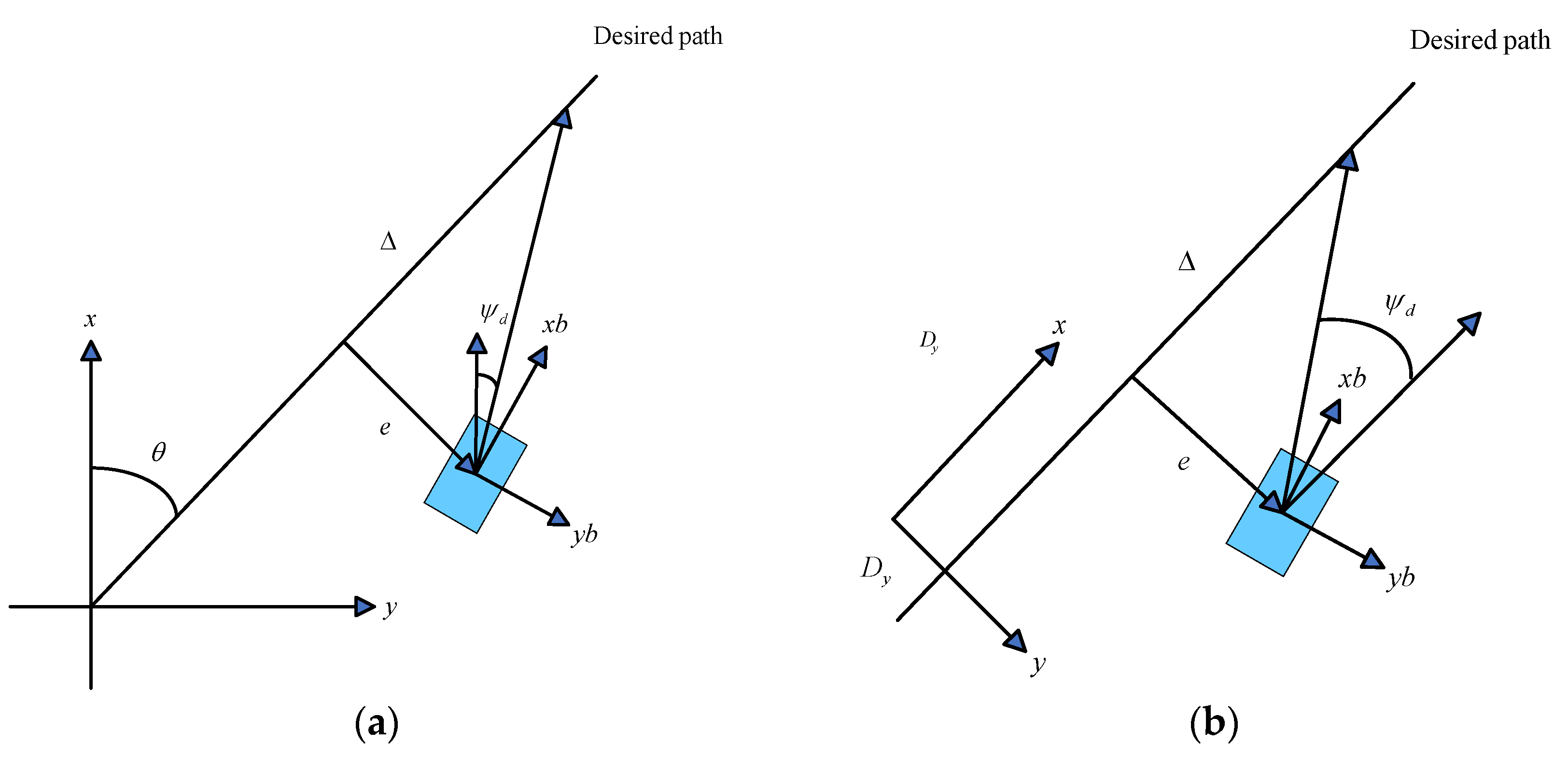
3.1. LOS
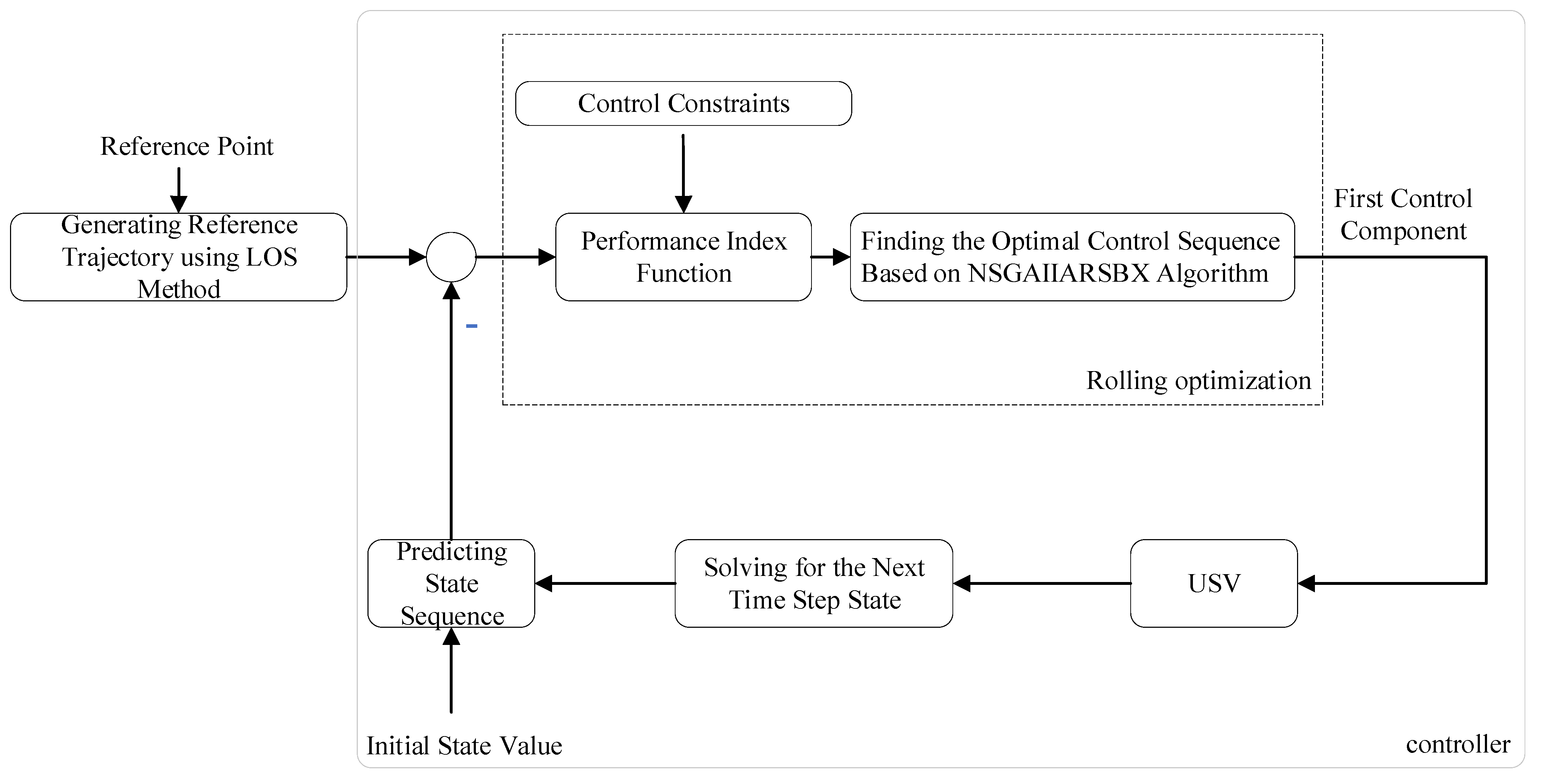
3.2. Controller
3.2.1. MPC
3.2.2. Constraints
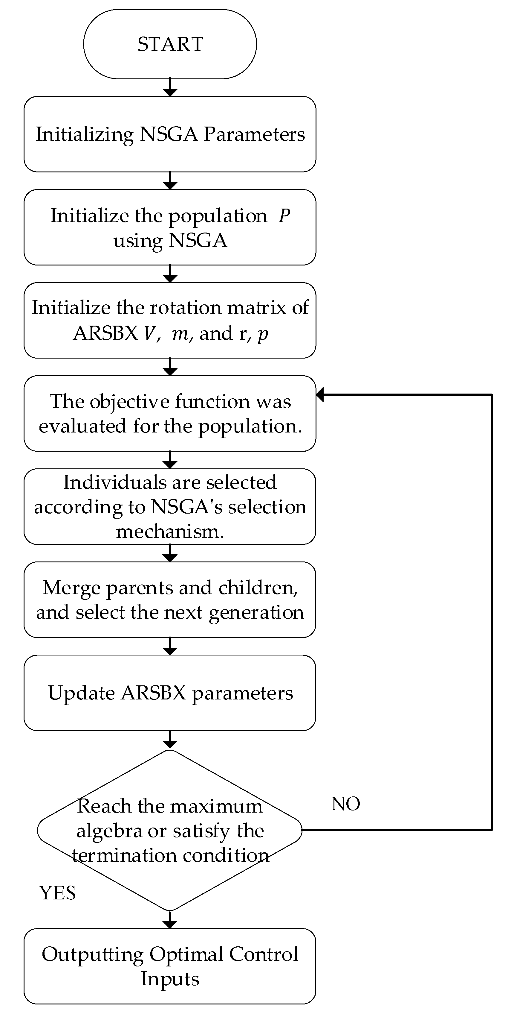
3.2.3. NSGAII
- Initialize population , mean vector , and rotation matrix . Generate an initial population with population size . For each individual in the population, calculate the objective function values . For multi-objective optimization, there will be multiple objectives.
- Non-dominated sorting and parent selection. Perform non-dominated sorting to divide the population into fronts and compute crowding distance for each individual to ensure diversity in the population. Select individuals from the current population to serve as parents for crossover.
- Integrating ARSBX crossover and mutation. Select pairs of parents for crossover and use ARSBX to generate offspring. Decide whether to use the rotation matrix based on probability ; if , use the identity matrix and zero mean vector:
- NSGA selection and sorting remain unchanged. Merge the parent population and offspring population:
- Repeat the above steps until the maximum generation is reached or another stopping criterion is satisfied.
3.2.4. Stability
4. Results
4.1. Scenario 1
4.2. Scenario 2
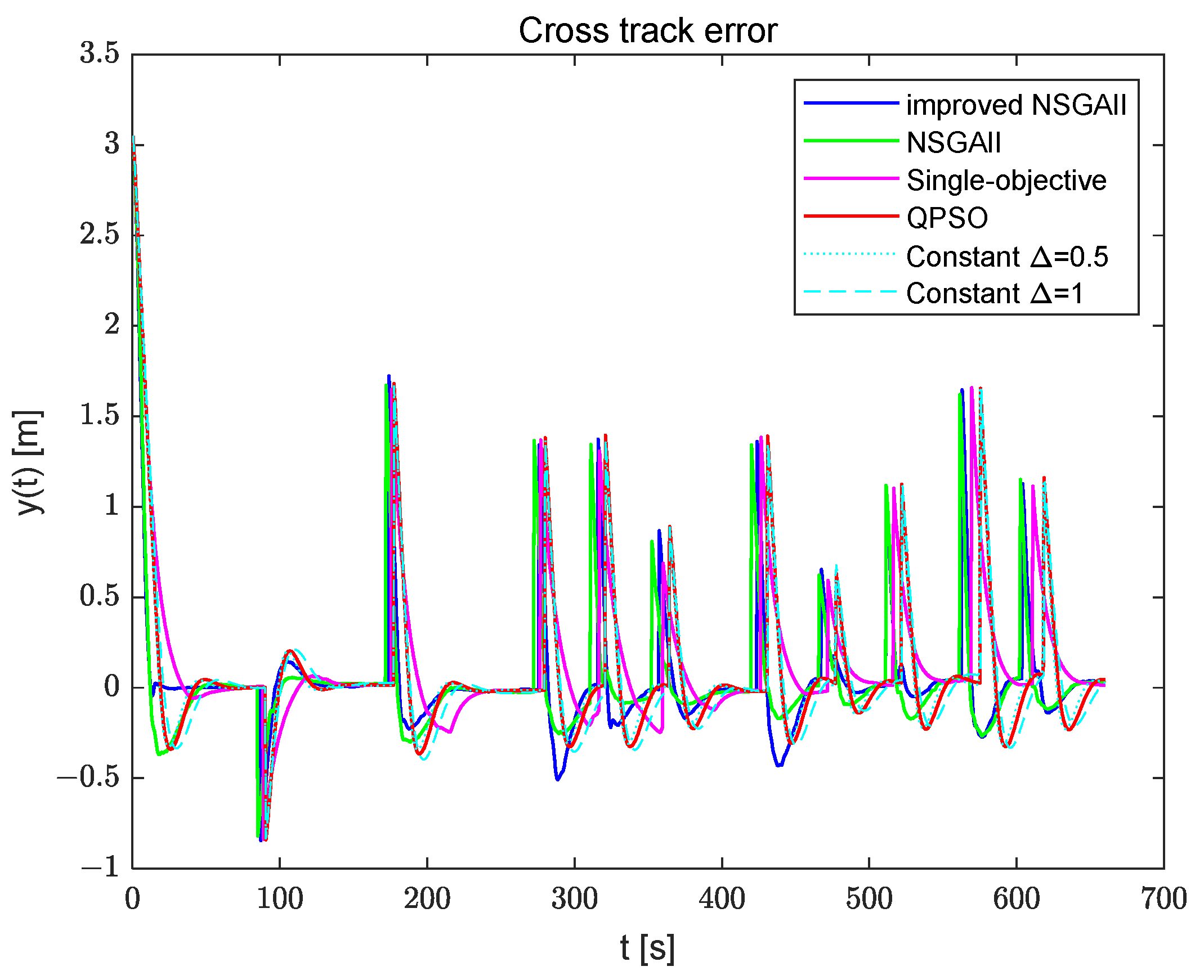
- The MPC algorithm with variable look-ahead distance demonstrates superior cross-track error performance compared to the fixed look-ahead distance algorithm, validating the effectiveness of this approach.
- A comparison between multi-objective and single-objective algorithms in terms of trajectory tracking performance shows that the multi-objective approach based on the improved NSGAII algorithm achieves a balanced consideration of both cross-track error and USV tracking speed, resulting in reduced cross-track error.
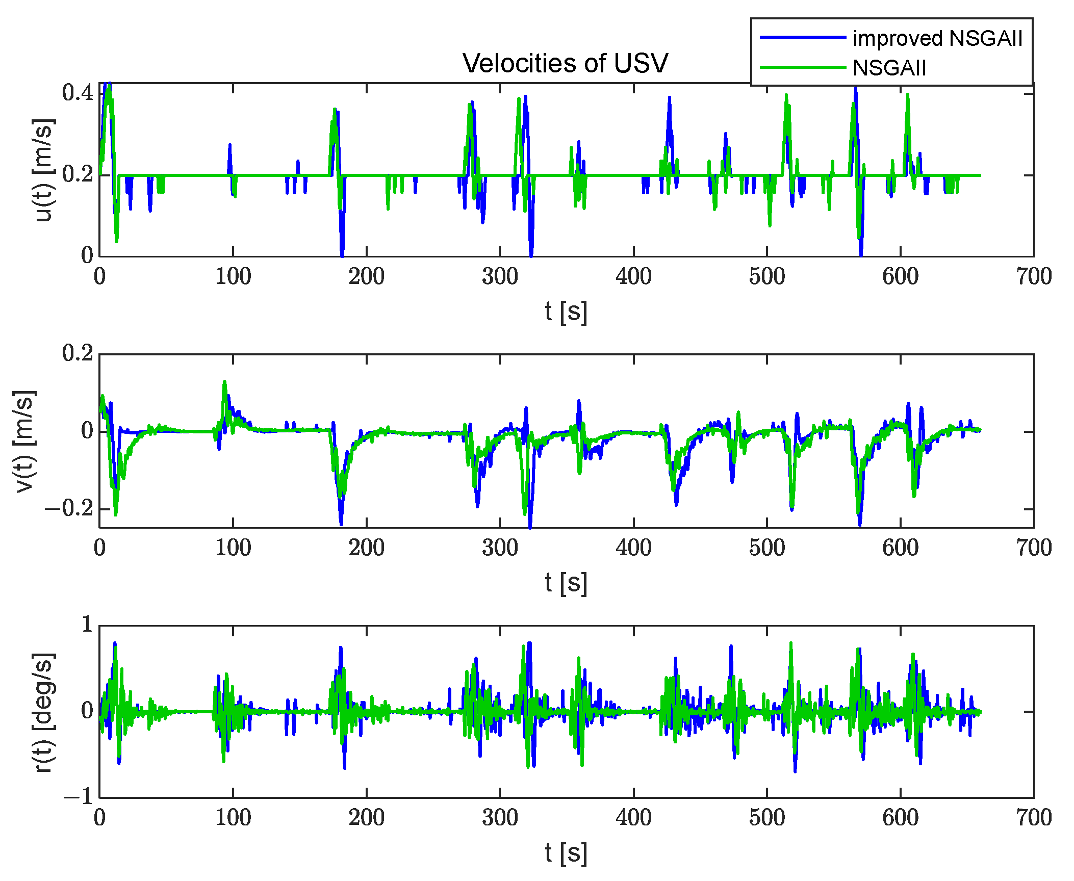
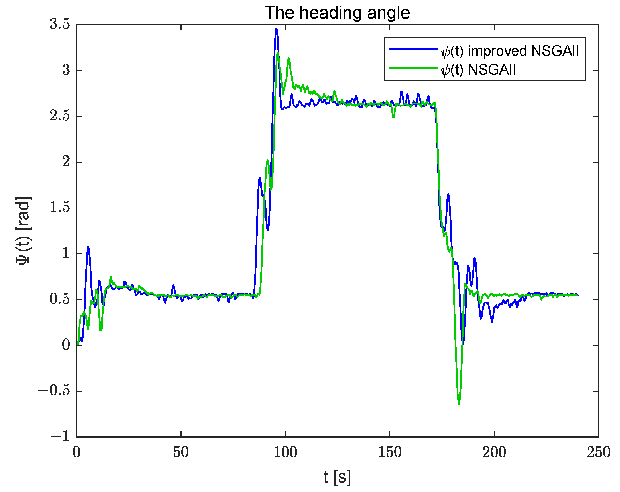
- By integrating an adaptive rotation-based simulated binary crossover and enhancing the non-dominated sorting method in the NSGAII algorithm, the improved NSGAII demonstrates superior tracking performance with reduced computation time, as observed from the trajectory tracking results.
5. Conclusions
Author Contributions
Funding
Institutional Review Board Statement
Informed Consent Statement
Data Availability Statement
Conflicts of Interest
References
- Yu, K.; Liang, X.-F.; Li, M.-Z.; Chen, Z.; Yao, Y.-L.; Li, X.; Zhao, Z.-X.; Teng, Y. USV path planning method with velocity variation and global optimisation based on AIS service platform. Ocean Eng. 2021, 236, 109560. [Google Scholar] [CrossRef]
- Barrera, C.; Padron, I.; Luis, F.S.; Llinas, O. Trends and challenges in unmanned surface vehicles (Usv): From survey to shipping. TransNav Int. J. Mar. Navig. Saf. Sea Transp. 2021, 15, 135–142. [Google Scholar] [CrossRef]
- Ashrafiuon, H.; Muske, K.R.; McNinch, L.C. Review of nonlinear tracking and setpoint control approaches for autonomous underactuated marine vehicles. In Proceedings of the 2010 American control Conference, Baltimore, MD, USA, 30 June–2 July 2010; pp. 5203–5211. [Google Scholar]
- Huixi, X.; Jiang, C. Heterogeneous oceanographic exploration system based on USV and AUV: A survey of developments and challenges. J. Univ. Chin. Acad. Sci. 2021, 38, 145–159. [Google Scholar]
- Lin, M.; Zhang, Z.; Pang, Y.; Lin, H.; Ji, Q. Underactuated USV path following mechanism based on the cascade method. Sci. Rep. 2022, 12, 1461. [Google Scholar] [CrossRef] [PubMed]
- Mou, J.; He, Y.; Zhang, B.; Li, S.; Xiong, Y. Path following of a water-jetted USV based on maneuverability tests. J. Mar. Sci. Eng. 2020, 8, 354. [Google Scholar] [CrossRef]
- Svec, P.; Thakur, A.; Shah, B.C.; Gupta, S.K. USV trajectory planning for time varying motion goals in an environment with obstacles. In Proceedings of the International design Engineering Technical Conferences and Computers and Information in engineering Conference, Chicago, IL, USA, 12–15 August 2012; Volume 45035, pp. 1297–1306. [Google Scholar]
- Do, K. Global robust adaptive path-tracking control of underactuated ships under stochastic disturbances. Ocean Eng. 2016, 111, 267–278. [Google Scholar] [CrossRef]
- Xiao, C.; Zhong, L.; Jianqiang, Z.; Dechao, Z.; Jiao, D. Adaptive sliding-mode path following control system of the underactuated USV under the influence of ocean currents. J. Syst. Eng. Electron. 2018, 29, 1271–1283. [Google Scholar]
- Johnson, M.A.; Moradi, M.H. PID Control; Springer: London, UK, 2005; pp. 47–107. [Google Scholar]
- Liu, Y.; Bu, R.; Gao, X. Ship trajectory tracking control system design based on sliding mode control algorithm. Pol. Marit. Res. 2018, 25, 26–34. [Google Scholar] [CrossRef]
- Yang, Z.K.; Zhong, W.B.; Feng, Y.B.; Sun, B. Unmanned surface vehicle track control based on improved LOS and ADRC. Chin. J. Ship Res. 2021, 16, 121–127. [Google Scholar]
- Bassam, A.M.; Phillips, A.B.; Turnock, S.R.; Wilson, P.A. Artificial neural network based prediction of ship speed under operating conditions for operational optimization. Ocean Eng. 2023, 278, 114613. [Google Scholar] [CrossRef]
- Beşikçi, E.B.; Arslan, O.; Turan, O.; Ölçer, A. An artificial neural network based decision support system for energy efficient ship operations. Comput. Oper. Res. 2016, 66, 393–401. [Google Scholar] [CrossRef]
- Sun, W.; Gao, X.; Yu, Y. Dual Deep Neural Networks for Improving Trajectory Tracking Control of Unmanned Surface Vehicle. In Proceedings of the 2020 Chinese Automation Congress (CAC), Shanghai, China, 6–8 November 2020; pp. 3441–3446. [Google Scholar]
- Sun, W.; Gao, X. Deep Learning-Based Trajectory Tracking Control for Unmanned Surface Vehicle. Math. Probl. Eng. 2021, 2021, 8926738. [Google Scholar]
- Zhang, G.; Zhang, X.; Zheng, Y. Adaptive neural path-following control for underactuated ships in fields of marine practice. Ocean Eng. 2015, 104, 558–567. [Google Scholar] [CrossRef]
- Tran, H.A.; Johansen, T.A.; Negenborn, R.R. Distributed MPC for autonomous ships on inland waterways with collaborative collision avoidance. arXiv 2024, arXiv:2403.00554. [Google Scholar]
- Qiang, H.; Jin, S.; Feng, X.; Xue, D.; Zhang, L. Model predictive control of a shipborne hydraulic parallel stabilized platform based on ship motion prediction. IEEE Access 2020, 8, 181880–181892. [Google Scholar] [CrossRef]
- Han, X.; Zhang, X. Tracking control of ship at sea based on MPC with virtual ship bunch under Frenet frame. Ocean Eng. 2022, 247, 110737. [Google Scholar] [CrossRef]
- Zhang, M.; Hao, S.; Wu, D.; Chen, M.-L.; Yuan, Z.-M. Time-optimal obstacle avoidance of autonomous ship based on nonlinear model predictive control. Ocean Eng. 2022, 266, 112591. [Google Scholar] [CrossRef]
- Dong, Z.; Chen, L.; Chen, P.; Mou, J. Model Predictive Control for Ship Path Tracking with Disturbances. In Proceedings of the 2023 IEEE International Conference on Unmanned Systems (ICUS), Hefei, China, 13–15 October 2023; pp. 1487–1492. [Google Scholar]
- Zhou, X.; Wu, Y.; Huang, J. MPC-based path tracking control method for USV. In Proceedings of the 2020 Chinese Automation Congress (CAC), Shanghai, China, 6–8 November 2020; pp. 1669–1673. [Google Scholar]
- Fossen, T.I. Marine Control Systems–Guidance, Navigation, and Control of Ships, Rigs and underwater Vehicles; Marine Cybernetics: Trondheim, Norway, 2002; ISBN 82-92356-00-2. [Google Scholar]
- Guan, G.; Wang, L.; Geng, J.; Zhuang, Z.; Yang, Q. Parametric automatic optimal design of USV hull form with respect to wave resistance and seakeeping. Ocean Eng. 2021, 235, 109462. [Google Scholar] [CrossRef]
- Fredriksen, E.; Pettersen, K.Y. Global κ-exponential way-point maneuvering of ships: Theory and experiments. Automatica 2006, 42, 677–687. [Google Scholar] [CrossRef]
- Gu, N.; Wang, D.; Peng, Z.; Wang, J.; Han, Q.-L. Advances in line-of-sight guidance for path following of autonomous marine vehicles: An overview. IEEE Trans. Syst. Man Cybern. Syst. 2022, 53, 12–28. [Google Scholar] [CrossRef]
- Dong, Z.; Zhang, Z.; Qi, S.; Zhang, H.; Li, J.; Liu, Y. Autonomous cooperative formation control of underactuated USVs based on improved MPC in complex ocean environment. Ocean Eng. 2023, 270, 113633. [Google Scholar] [CrossRef]
- Hu, L.; Zhang, M.; Li, G.; Yuan, Z.; Bi, J.; Guo, Y. Multi-objective model predictive control for ship roll motion with gyrostabilizers. Ocean Eng. 2024, 313, 119412. [Google Scholar] [CrossRef]
- Liu, S.; Yu, Z.; Wang, T.; Chen, Y.; Zhang, Y.; Cai, Y. MPC-Based Collaborative Control of Sail and Rudder for Unmanned Sailboat. J. Mar. Sci. Eng. 2023, 11, 460. [Google Scholar] [CrossRef]
- Fossen, T.I.; Breivik, M.; Skjetne, R. Line-of-sight path following of underactuated marine craft. IFAC Proc. Vol. 2003, 36, 211–216. [Google Scholar] [CrossRef]
- Ma, H.; Zhang, Y.; Sun, S.; Liu, T.; Shan, Y. A comprehensive survey on NSGA-II for multi-objective optimization and applications. Artif. Intell. Rev. 2023, 56, 15217–15270. [Google Scholar] [CrossRef]
- Verma, S.; Pant, M.; Snasel, V. A comprehensive review on NSGA-II for multi-objective combinatorial optimization problems. IEEE Access 2021, 9, 57757–57791. [Google Scholar] [CrossRef]
- Deb, K.; Pratap, A.; Agarwal, S.; Meyarivan, T. A fast and elitist multiobjective genetic algorithm: NSGA-II. IEEE Trans. Evol. Comput. 2002, 6, 182–197. [Google Scholar] [CrossRef]
- Pan, L.; Xu, W.; Li, L.; He, C.; Cheng, R. Adaptive simulated binary crossover for rotated multi-objective optimization. Swarm Evol. Comput. 2021, 60, 100759. [Google Scholar] [CrossRef]
- Lee, J.W. Exponential stability of constrained receding horizon control with terminal ellipsoid constraints. IEEE Trans. Autom. Control 2000, 45, 83–88. [Google Scholar]


| Parameters | Value | Unit | Parameters | Value | Unit |
|---|---|---|---|---|---|
| 23.8 | kg | 0.1079 | N · s/m | ||
| 0.046 | m | −0 | kg | ||
| 1.76 | kg · m | 0.1052 | N · s/m | ||
| −0.7225 | N · s/m | −0 | kg | ||
| −2.0 | kg | −0.5 | N · s/m | ||
| −0.8612 | N · s/m | −1.0 | kg | ||
| −10 | kg |
| Approach | Average Single Run Time (s) |
|---|---|
| NSGAII | 2.557 |
| Improved NSGAII | 0.89 |
| QPSO | 2.210 |
| Controller Parameter | Value | Unit |
|---|---|---|
| 45 | ||
| 15 | ||
| [2, 1.5] | [N, N · m] | |
| [−2, −1.5] | [N, N · m] | |
| [1, −0.2] | ||
| 4 | ||
| 40 | ||
| 5 | ||
| ] | [10, 6.32,5] | |
| The range of surge velocity of USV u | [0, 0.5] | m/s |
| Method | Sum of the Absolute Values of the Cross-Track Errors (m) |
|---|---|
| NSGAII | 220.52 |
| Improved NSGAII | 204.31 |
| Improved NSGAII and look-ahead distance = 1 | 298.57 |
| Improved NSGAII and constant look-ahead distance = 0.5 | 246.81 |
| Single-objective | 294.70 |
| QPSO | 225.26 |
| Method | Sum of the Absolute Values of the Cross-Track Errors (m) |
|---|---|
| NSGAII | 78.67 |
| Improved NSGAII | 72.17 |
| Improved NSGAII and look-ahead distance = 1 | 104.68 |
| Improved NSGAII and constant look-ahead distance = 0.5 | 79.54 |
| Single-objective | 112.29 |
| QPSO | 79.61 |
Disclaimer/Publisher’s Note: The statements, opinions and data contained in all publications are solely those of the individual author(s) and contributor(s) and not of MDPI and/or the editor(s). MDPI and/or the editor(s) disclaim responsibility for any injury to people or property resulting from any ideas, methods, instructions or products referred to in the content. |
© 2024 by the authors. Licensee MDPI, Basel, Switzerland. This article is an open access article distributed under the terms and conditions of the Creative Commons Attribution (CC BY) license (https://creativecommons.org/licenses/by/4.0/).
Share and Cite
Guo, Y.; Zhu, Q.; Mou, J. The Path Tracking Control of Unmanned Surface Vehicles Based on an Improved Non-Dominated Sorting Genetic Algorithm II-Based Multi-Objective Nonlinear Model Predictive Control Method. J. Mar. Sci. Eng. 2024, 12, 2188. https://doi.org/10.3390/jmse12122188
Guo Y, Zhu Q, Mou J. The Path Tracking Control of Unmanned Surface Vehicles Based on an Improved Non-Dominated Sorting Genetic Algorithm II-Based Multi-Objective Nonlinear Model Predictive Control Method. Journal of Marine Science and Engineering. 2024; 12(12):2188. https://doi.org/10.3390/jmse12122188
Chicago/Turabian StyleGuo, Yunzhe, Qidan Zhu, and Jinyou Mou. 2024. "The Path Tracking Control of Unmanned Surface Vehicles Based on an Improved Non-Dominated Sorting Genetic Algorithm II-Based Multi-Objective Nonlinear Model Predictive Control Method" Journal of Marine Science and Engineering 12, no. 12: 2188. https://doi.org/10.3390/jmse12122188
APA StyleGuo, Y., Zhu, Q., & Mou, J. (2024). The Path Tracking Control of Unmanned Surface Vehicles Based on an Improved Non-Dominated Sorting Genetic Algorithm II-Based Multi-Objective Nonlinear Model Predictive Control Method. Journal of Marine Science and Engineering, 12(12), 2188. https://doi.org/10.3390/jmse12122188