Numerical Simulation of Wave-Induced Scour in Front of Vertical and Inclined Breakwaters

Abstract

The erosion of the seabed in front of shoreline structures due to wave action is a critical concern. While previous models accurately depict fluid and sediment interactions, they each have limitations and require significant computational resources, especially when simulating complex processes. This study proposed and validated a numerical model for simulating wave-induced sediment transport by integrating three key components: (1) a main solver based on large eddy simulation that includes the porosity of permeable materials, (2) a volume of fluid module to track the air–water surface, and (3) a sediment transport module that includes both bedload and suspended load to compute sediment concentrations and seabed changes. The model was validated against previously published experimental data, demonstrating its accuracy in capturing both wave motion and seabed profile changes induced by sediment transport. Furthermore, the numerical model was applied to study the effects of varying breakwater slopes on sediment seabed profile changes. The results show that steeper breaker slopes led to more concentrated wave energy near the structure, resulting in deeper scouring and higher sediment displacement. These results indicate that the proposed model is a valuable tool for coastal engineering applications, particularly for designing breakwaters, to mitigate sediment erosion and improve sediment stability.

1. Introduction

The scouring of the seabed in front of or around coastal structures owing to the action of ocean water waves is crucial in the coastal engineering field [1]. Japan has a total coastline length of more than 800 km. Therefore, predicting scouring patterns and depths is paramount to coastal scientists and engineers in Japan [2].

Scour processes occur (1) in front of the structure along the length of the trunk section and (2) around the breakwater head. When waves attack the breakwater at right angles, scouring in front of the breakwater is a two-dimensional process. Head scouring is always a three-dimensional process [3]. Scholars have developed solvers using different methods to conduct numerical simulations in response to the problem of sediment erosion in breakwaters caused by waves. The most typically used methods are two-phase flow and empirical formulas.

In two-phase flow methods, fluid and sediment are treated as two separate phases and are modeled as either continuous or discrete systems. Hajivalie et al. [4] used a two-dimensional Euler–Lagrange model to simulate scour in front of breakwaters with fluid dynamics governed by Reynolds-averaged Navier–Stokes (RANS) equations and sediment transport described as discrete particles moving in various modes. Yeganeh-Bakhtiary et al. [5] used particle-based coupling weakly compressible smoothed particle hydrodynamics for fluid flow and the discrete element method for sediment transport to identify new recirculation mechanisms shaping the scour profiles. Chauchat et al. [6] extended the two-phase EulerFoam solver of OpenFOAM’s to model sediment as a continuum with granular flow rheology. Li and Chen [7] proposed a two-phase mixture model to handle bedload and suspended load, improving computational efficiency while maintaining accuracy in predicting complex scour patterns. These models offer accurate simulations of fluid–sediment interactions; however, they are computationally expensive and time-consuming, particularly when capturing complex processes such as bedload transport, suspended sediment transport, and topographic changes.

Empirical formula methods estimate sediment transport using various adaptable formulas to predict the bedload and suspended load. A well-known example is the Meyer-Peter and Müller equation [8], which is used for bedload transport in gravel beds under steady flow. For a suspended load, the Rouse [9] equation predicts the vertical distribution of sediment concentration based on the particle settling and flow shear velocities. Additionally, the Engelund and Hansen [10] formula estimates the total sediment transport by combining the bedload and suspended load. However, these formulas are limited by their applicability to specific flow conditions, and often struggle with turbulent or unsteady flows [8]. Moreover, appropriate calibration and experimental validation are essential to ensure accuracy.

Recently, Hou et al. [11] used FS3M, a three-dimensional coupled fluid–structure–sediment–seabed interaction model (FS3M), developed by Nakamura and Yim [12]. This numerical code simulates the dynamic interaction between the fluid flow, object motion, seabed profile evolution, and seabed response under ocean waves. This model uses the grid method, a finite-difference method, for solving and calculation. In this model, the wave-field component was extended to incorporate the infiltration flow within the seabed. The pressure and velocity generated at the seabed surface are subsequently fed into the seabed model. The wave-field and seabed interactions were coupled using a one-way coupling approach.

This study aims to validate a numerical model [11,12] for simulating wave-induced sediment transport by integrating three main components: wave dynamics, sediment transport processes, and bed morphology changes. The model was validated against the experimental data reported in [1], thereby demonstrating its accuracy in capturing wave dynamics and sediment-induced seabed changes. Furthermore, the model was applied to investigate the influence of breakwater slope on sediment scour and deposition.

The manuscript is structured as follows: Section 1 introduces the study, including the background and motivation, emphasizing the challenges of simulating wave–sediment interactions. Moreover, a literature review on two-phase flow and empirical formula methods is provided. Section 2 describes the numerical model, including governing equations, porosity handling, volume of fluid (VOF) methods, and sediment transport processes. Section 3 presents the results of the validation of the model using experimental data and discusses the model’s performance in simulating wave motion and seabed profile changes. Section 4 presents the model’s application to study the impact of varying breakwater slopes on sediment transport, and analyzes how slope variations affect scour and deposition patterns. Finally, Section 5 summarizes key findings and future research

2. Materials and Methods

The FS3M integrates two core components essential for this study. The wave field model (detailed in Section 2.1) focuses on simulating fluid dynamics using the VOF method to track the air–water interface, ensuring accurate wave behavior representation. The sediment transport model (detailed in Section 2.2) handles both bedload and suspended load transport and computes sediment concentrations and seabed profile changes driven by wave action. Combined, these components allow the model to capture the complex interactions between wave motion, sediment transport, and seabed evolution. Therefore, FS3M is an effective tool for coastal engineering research.

2.1. Wave Field Model

In the wave field model, the continuity and Navier–Stokes (N–S) equations for incompressible viscous fluids are generally used as governing equations. When the VOF method is used to track the gas–liquid interface, the advection equation of the VOF function is included in the governing equations. The main solver is based on a large-eddy simulation (LES), which directly calculates large-scale vortices called the grid scale (GS) while modeling smaller-scale vortices known as the sub-grid scale, which is expected to be universal. Consequently, the continuity and N-S equations in LES are spatially filtered versions known as grid-filtered equations. In this solver, the governing equations are described by Equations (1)–(3).

More specifically, Equation (1) ensures mass conservation within the porous medium by accounting for porosity $m$ and external source terms $q^{\ast }$. Equation (2) governs momentum conservation, incorporating external forces, viscous stresses, and interactions within the porous medium. Equation (3) tracks the evolution of the volume fraction F, essential for capturing the dynamics of the air–water interface. Together, these equations provide a comprehensive framework for modeling fluid dynamics and wave interactions in permeable materials.

$${\displaystyle \frac{\mathsf{\partial }m}{\mathsf{\partial }t}}+{\displaystyle \frac{\mathsf{\partial }\left(m\overline{v_j}\right)}{\mathsf{\partial }{x}_j}}=q^{\ast }$$

(1)

$${\displaystyle \frac{\mathsf{\partial }\left[\{m+C_A(1-m)\}\overline{v_i}\right]}{\mathsf{\partial }t}}+{\displaystyle \frac{\mathsf{\partial }\left(m\overline{v_i}\overline{v_j}\right)}{\mathsf{\partial }{x}_j}}=-{\displaystyle \frac{m}{\widehat{\rho }}}{\displaystyle \frac{\mathsf{\partial }\overline{p}}{\mathsf{\partial }{x}_i}}+m{g}_i+{\displaystyle \frac{m}{\widehat{\rho }}}\left(f_i^s+R_i+f_i^{ab}\right)+{\displaystyle \frac{1}{\widehat{\rho }}}{\displaystyle \frac{\mathsf{\partial }}{\mathsf{\partial }{x}_j}}\left(2m\widehat{\mu }\overline{D_{ij}}\right)+{\displaystyle \frac{\mathsf{\partial }}{\mathsf{\partial }{x}_j}}\left(-m{\tau }_{ij}^a\right)+Q_i-m\beta \overline{v_i}$$

(2)

$${\displaystyle \frac{\mathsf{\partial }\left(mF\right)}{\mathsf{\partial }t}}+{\displaystyle \frac{\mathsf{\partial }\left(m\overline{v_j}F\right)}{\mathsf{\partial }{x}_j}}=F{q}^{\ast }$$

(3)

In the equations, x and y represent the horizontal coordinates (m), z is the upward coordinate (m), t represents time (s), $\overline{v_j}$ is the GS component of velocity (m/s), and $\overline{p}$ is the GS component of pressure (Pa). Regarding the fluid properties, F is the VOF function representing the fluid fraction in each computational grid cell, and 0 < F < 1 indicates the gas–liquid interface. $g_i$ is the gravitational acceleration vector (m/s²); $\widehat{\rho }$ is the fluid density (kg/m³), calculated as $\widehat{\rho }=F{\rho }_w+\left(1-F\right){\rho }_a$, and ${\rho }_w$ and ${\rho }_a$ are the densities of water and air, respectively. Moreover, $\widehat{\mu }$ is the fluid viscosity (Pa.s), given by $\widehat{\mu }=F{\mu }_w+(1-F){\mu }_a$, where ${\mu }_w$ and ${\mu }_a$ are the viscosities of water and air, respectively. Furthermore, m represents the porosity of permeable materials, $C_A$ denotes the added mass coefficient for permeable materials [13], $f_i^s$ (N/m³) refers to the continuum surface model related to surface tension at the gas–liquid interface [14], $R_i$ (N/m³) denotes the linear/non-linear drag vector owing to permeable materials, and $f_i^{ab}$ (N/m³) is the fluid–structure interaction force vector. $\overline{D_{ij}}$ (1/s) is the deformation tensor for the GS turbulence model, calculated as $\overline{D_{ij}}=\left(\mathsf{\partial }\overline{v_j}/\mathsf{\partial }{x}_i+\mathsf{\partial }\overline{v_i}/\mathsf{\partial }{x}_j\right)/2$, where ${\tau }_{ij}^a$ (Pa) represents a coherent structure model [15]. In the wave-generating properties, $Q_i$ (m³/s³) is the source vector of the wave, and $q^{\ast }$ (kg/m³/s) is the time-averaged source strength per unit volume of the wave source [16]. $\beta$ is the reduction coefficient of the reduction domain.

2.2. Sediment Transport Model

Note that sediment transport provides the potential for a change in the surface morphology of the seabed. Our solver describes the sediment transport model as a sediment transport (ST) module. The ST module includes the following: (1) a sediment continuity equation for calculating morphological changes due to bedload and suspended sediment transport; (2) a bedload transport model that calculates the amount of bedload, constructed based on Roulund et al. [17]; (3) a suspended load transport model that calculates the distribution of suspended load concentration considering the lifting of bottom sediment, advection diffusion, and settling; and (4) a slope collapse model that calculates the slope collapse of the moving bed, constructed based on Roulund et al. [17].

2.2.1. Continuity Equation for Bedload and Suspended Sediment Transport

The continuity equation for sediment transport is expressed as follows:

$${\displaystyle \frac{\mathsf{\partial }{z}_s}{\mathsf{\partial }t}}+{\displaystyle \frac{1}{1-m}}\left({\displaystyle \frac{\mathsf{\partial }{q}_x}{\mathsf{\partial }x}}+{\displaystyle \frac{\mathsf{\partial }{q}_y}{\mathsf{\partial }y}}+P_N+q_{zb}^s\right)=0$$

(4)

where $z_s$ (m) is the height of the moving bed surface from the reference surface; $m$ is the porosity; $q_x$ and $q_y$ (m²/s) are the bedload transport rate per unit width and unit time in the x and y direction, respectively; $P_N$ (kg/m²/s) is the sediment pick-up function; and $q_{zb}^s$ (kg/m²/s) is the suspended sediment transport flux due to settling in the z-direction on the moving bed surface. Therefore, if $q_x$, $q_y$, $P_N$, and $q_{zb}^s$ can be determined, the time change in $z_s$ can be calculated using Equation (4).

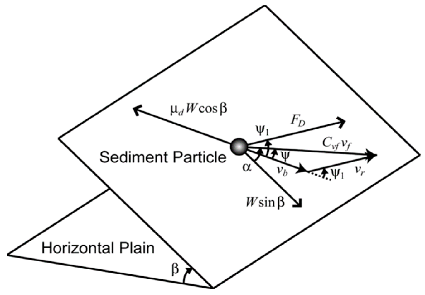
2.2.2. Bedload Sediment Transport Model

The bedload transport rate $q_i$ in the i-direction per unit width and unit time can be obtained using Equation (5) [18] as follows:

$$q_i={\displaystyle \frac{1}{6}}\pi d_{50}{P}_{EF}{v}_{bi}$$

(5)

here, $P_{EF}$ represents the proportion of bed particles in motion owing to bedload transport, $v_b$ (m/s) is the transportation velocity of sediment particles, $v_{bi}$ is the i-direction component of $v_b$, and $d_{50}$ (m) is the median diameter of sediment particles. Therefore, if $P_{EF}$ and $v_{bi}$ can be determined, $q_x$ and $q_y$ in Equation (4) can also be determined. First, $P_{EF}$ is given as follows:

$$P_{EF}=\left\{\begin{array}{ll}0& if{\tau }_{\ast }\le {\tau }_{\ast c}\\ {\displaystyle \frac{6}{\pi {\mu }_d}}\left({\tau }_{\ast }-{\tau }_{\ast c}\right)& if{\tau }_{\ast }>{\tau }_{\ast c}\end{array}\right.$$

(6)

$${\tau }_{\ast }={\displaystyle \frac{v_f^2}{\left({\rho }_s/{\rho }_w-1\right)g{d}_{50}}}$$

(7)

here, ${\mu }_d$ is the dynamic friction coefficient of the bed particles (where ${\mu }_d$ = tan${\theta }_d$, and ${\theta }_d$ is the dynamic friction angle), ${\tau }_{\ast }$ is the shields parameter, and ${\tau }_{\ast c}$ is critical shields number, which is discussed later in the manuscript. Additionally, the friction velocity $v_f$ (m/s) can be calculated as follows:

$${\displaystyle \frac{v_{surf}}{v_f}}=2{\displaystyle {\int }_0^{z_{zel}^{+}}1/\left[1+\sqrt{1+4{\kappa }^2{\left(z^{\prime }+△z^{+}\right)}^2{\left[1-\exp \left\{-\left(z^{\prime }+△z^{+}\right)/A\right\}\right]}^2}\right]}d{z}^{\prime }$$

(8)

where $v_{surf}$ (m/s) is the tangential flow velocity at a height $z_{vel}$ from the bed surface, $\kappa$ is the von Kármán constant, and $A$ is the van Driest damping function coefficient. $k_s^{+}$ is the roughness Reynolds number and $△z^{+}$ is given by $△z^{+}=0.9\left\{\sqrt{k_s^{+}}-k_s^{+}\exp \left(-k_s^{+}/6\right)\right\}$.

To calculate the i-direction component of the particle velocity $v_{bi}$ (m/s) in Equation (5), it is necessary to analyze the forces acting on a non-cohesive, uniformly sized, spherical sediment particle resting on a sloping bed. As illustrated in Figure 1, the gravitational force W (N) is decomposed into two components—$W\sin \beta$ (N), which acts parallel to the slope and drives downslope motion, and $W\cos \beta$ (N), which acts perpendicular to the slope and contributes to frictional resistance. The frictional resistance is represented by ${\mu }_{d}W\cos \beta$ (N), where ${\mu }_d$ is the dynamic friction coefficient. Additionally, the drag force $F_D$ (N) from the flow further influences the particle’s movement. The particle motion also depends on its velocity relative to the surrounding fluid; the relative velocity between the particle and the fluid $v_r$ (m/s), the fluid velocity component along the slope $v_f$ (m/s), and the velocity component $v_b$ (m/s) that contributes to the bedload transport. Moreover, the centrifugal force $C_{vf}{v}_f$ (N) accounts for the rotational effects of the interaction between the particle and the fluid. Combined, these forces interact dynamically to determine whether the particle remains stationary or moves across the sloping bed.

The set of equations describing the motion of sediment particles, Equations (9)–(12), can be obtained based on the geometric relationships and Newton’s second law. These equations describe the necessary conditions for a sediment particle to overcome resistance and begin moving along the slope, where $\Psi$ (degree) reflects the alignment between the particle and fluid velocities, impacting the extent to which the fluid can effectively apply force to the particle; ${\Psi }_1$ (degree) shows the influence of the slope on the relative movement, which helps determine whether the particle overcomes the resistance to initiate motion. Equations (13) and (14) define the gravitational and drag forces, respectively. In these equations, the unknowns are $v_b$, $v_r$, $\Psi$, and ${\Psi }_1$. These variables can be determined iteratively using the Newton–Raphson method. After calculating $v_b$ and its direction, $\Psi$, that is, the value of $v_{bi}$, can be obtained.

$$F_D\cos {\Psi }_1+W\sin \beta \cos \left(\alpha -\Psi \right)={\mu }_{d}W\cos \beta$$

(9)

$$F_D\sin {\Psi }_1=W\sin \beta \sin \left(\alpha -\Psi \right)$$

(10)

$$v_r\sin {\Psi }_1=C_{vf}{v}_f\sin \Psi$$

(11)

$$v_r\cos {\Psi }_1+v_b=C_{vf}{v}_f\cos \Psi$$

(12)

$$W={\displaystyle \frac{1}{6}}\pi ({\rho }_s-{\rho }_w)g{d}_{50}^3$$

(13)

$$F_D={\displaystyle \frac{1}{8}}\pi \epsilon C_{D1}{\rho }_w{d}_{50}^2{v}_r^2=C_{FD}{v}_r^2$$

(14)

In addition, by analyzing the above forces, we can obtain the calculation formula for the critical Shields number ${\tau }_{\ast c}$, required in Equation (6). The critical Shields number for a sloping bed is expressed as in Equation (15).

$${\tau }_{\ast c}={\tau }_{\ast c0}\left(\cos \beta \sqrt{1-{\displaystyle \frac{{\sin }^2\alpha {\tan }^2\beta }{{\mu }_s^2}}}-{\displaystyle \frac{\cos \alpha \sin \beta }{{\mu }_s}}\right)$$

(15)

where $\beta$ (degree) is the bed slope angle, $\alpha$ (degree) is the angle of the force applied to the particle (relative to the bed), ${\mu }_s$ is the coefficient of static friction accounting for the particle’s resistance to sliding, ${\tau }_{\ast c0}$ is the critical Shields number for a horizontal bed, which can be determined using Iwagaki’s formula [19] or directly specified through numerical input. The second method was used in this study.

2.2.3. Suspended Sediment Transport Model

The concentration of suspended sediment $C$ (kg/m³) is determined using generalized advection–diffusion, which can also be applied to pores inside permeable materials.

$$m{\displaystyle \frac{\mathsf{\partial }C}{\mathsf{\partial }t}}+{\displaystyle \frac{\mathsf{\partial }}{\mathsf{\partial }{x}_j}}\left(q_j^C+q_j^D+q_j^S\right)=0$$

(16)

In this context, permeable materials are assumed to be riprap or wave-blocking blocks that allow suspended sediment infiltration. The terms $q_j^C$ (kg/m²/s), $q_j^D$ (kg/m²/s), and $q_j^S$ (kg/m²/s) represent the suspended sediment transport fluxes due to advection, diffusion, and settling, respectively, and are expressed in Equations (17)–(19).

$$q_j^C=m{v}_{j}C$$

(17)

$$q_j^D=-m{\epsilon }_s{\displaystyle \frac{\mathsf{\partial }C}{\mathsf{\partial }{x}_j}}$$

(18)

$$q_j^S=m{w}_{si}C$$

(19)

where ${\epsilon }_s$ (m²/s) is the turbulent diffusion coefficient for the suspended sediment, $w_{si}$ (m/s) is the settling velocity vector of the bed particles (=${\left[0 0 - w_s\right]}^T$), and $w_s$ (m/s) is the settling velocity of the bed particles, obtained using empirical formulas, such as Rubey’s equation. To solve Equation (16), Nielsen et al. [20] provided the boundary conditions at the mobile bed surface. Specifically, the suspended sediment transport flux by diffusion $q_j^D$ (kg/m²/s) is equal to the sediment pickup function $p^N$ (kg/m²/s), which is given as follows:

$$p^N=\left\{\begin{array}{ll}0\hfill & \mathrm{if} {\tau }_{\ast }<{\tau }_{\ast c}\hfill \\ C_p{\left({\displaystyle \frac{{\tau }_{\ast }-{\tau }_{\ast c}}{{\tau }_{\ast }}}\right)}^{1.5}{\displaystyle \frac{{\left(s-1\right)}^{0.6}{g}^{0.6}{d}^{0.8}}{{\nu }_w^{0.2}}}\hfill & \mathrm{if} {\tau }_{\ast }\ge {\tau }_{\ast c}\hfill \end{array}\right.$$

(20)

$C_p$ is a dimensionless parameter related to the bed particle pickup rate with a value of $C_p=0.00033$ for a steady flow [21]. Consequently, the value of $p^N$ in Equation (4) is determined using Equation (20), and the suspended sediment transport flux due to settling in the z-direction on the moving bed surface $q_{zb}^s$ (kg/m²/s) is determined using Equation (19). In addition, ${\tau }_{\ast c}$ considers the effects of the infiltration and exfiltration flows, pore water pressure, and cohesive forces.

2.2.4. Slope Failure Model

When the slope angle $\beta$ (degree) of the mobile bed exceeds the underwater angle of repose ${\theta }_r$ (degree) by a small angle ${\theta }_r^{+}$ (degree), slope collapse begins. The collapse continues even when the slope angle decreases below ${\theta }_r^{-}$ (degree) [22]. Based on this, Roulund et al. [17] established that in the previously mentioned sediment transport model, when the slope angle $\beta$ exceeds ${\theta }_r+{\theta }_r^{+}$, all bed particles collapse ($P_{EF}=1$). It is further assumed that under still water conditions ($v_f=0,\Psi ={\Psi }_1=180$°), the slope continues to collapse at a constant velocity in the downslope direction ($\alpha =180$°). Additionally, the effects of forces $F_L$ (N) and $F_w$ (N) during slope collapse are assumed to be negligible. Under these assumptions, and after substituting and $\alpha =\Psi ={\Psi }_1=180$° into Equations (9)–(12), and combining them with $W$ (N) and $F_D$ (N) in Equations (13) and (14), the average transport velocity of bed particles due to the slope collapse $v_b^{slide}$ (m/s) can be expressed as follows:

$$v_b^{slide}=\sqrt{{\displaystyle \frac{4}{3}}{\displaystyle \frac{d}{\epsilon C_{D1}}}\left({\rho }_s/{\rho }_w-1\right)g\left(\sin \beta -{\mu }_d\cos \beta \right)}$$

(21)

substituting Equations (21) and $P_{EF}=1$ into Equation (5), the slope collapse bedload transport rate $q_i^{slide}$ (m²/s) can be determined as follows:

$$q_i^{slide}={\displaystyle \frac{\pi }{3}}{C}_{slide}{d}_{50}\sqrt{{\displaystyle \frac{1}{3}}{\displaystyle \frac{d_{50}}{\epsilon C_{D1}}}\left({\rho }_s/{\rho }_w-1\right)g\left(\sin \beta -{\mu }_d\cos \beta \right)}$$

(22)

here, $C_{slide}$ (m/s) is a parameter introduced to control the velocity of slope failure. Based on the experimental results reported in [23], the value of $C_{slide}=290$ provides the best fit [24]. Additionally, $P_N=0$ and $q_{zb}^s=0$, when assuming that no sediment lifting or settling occurs during slope collapse. Then, the sediment continuity, Equation (4), can be applied using Equation (23).

$${\displaystyle \frac{\mathsf{\partial }{z}_s}{\mathsf{\partial }t}}+{\displaystyle \frac{1}{1-m}}\left({\displaystyle \frac{\mathsf{\partial }{q}_x^{slide}}{\mathsf{\partial }x}}+{\displaystyle \frac{\mathsf{\partial }{q}_y^{slide}}{\mathsf{\partial }y}}\right)=0$$

(23)

Therefore, the time variation owing to slope collapse in the z-axis direction can be calculated using Equations (22) and (23).

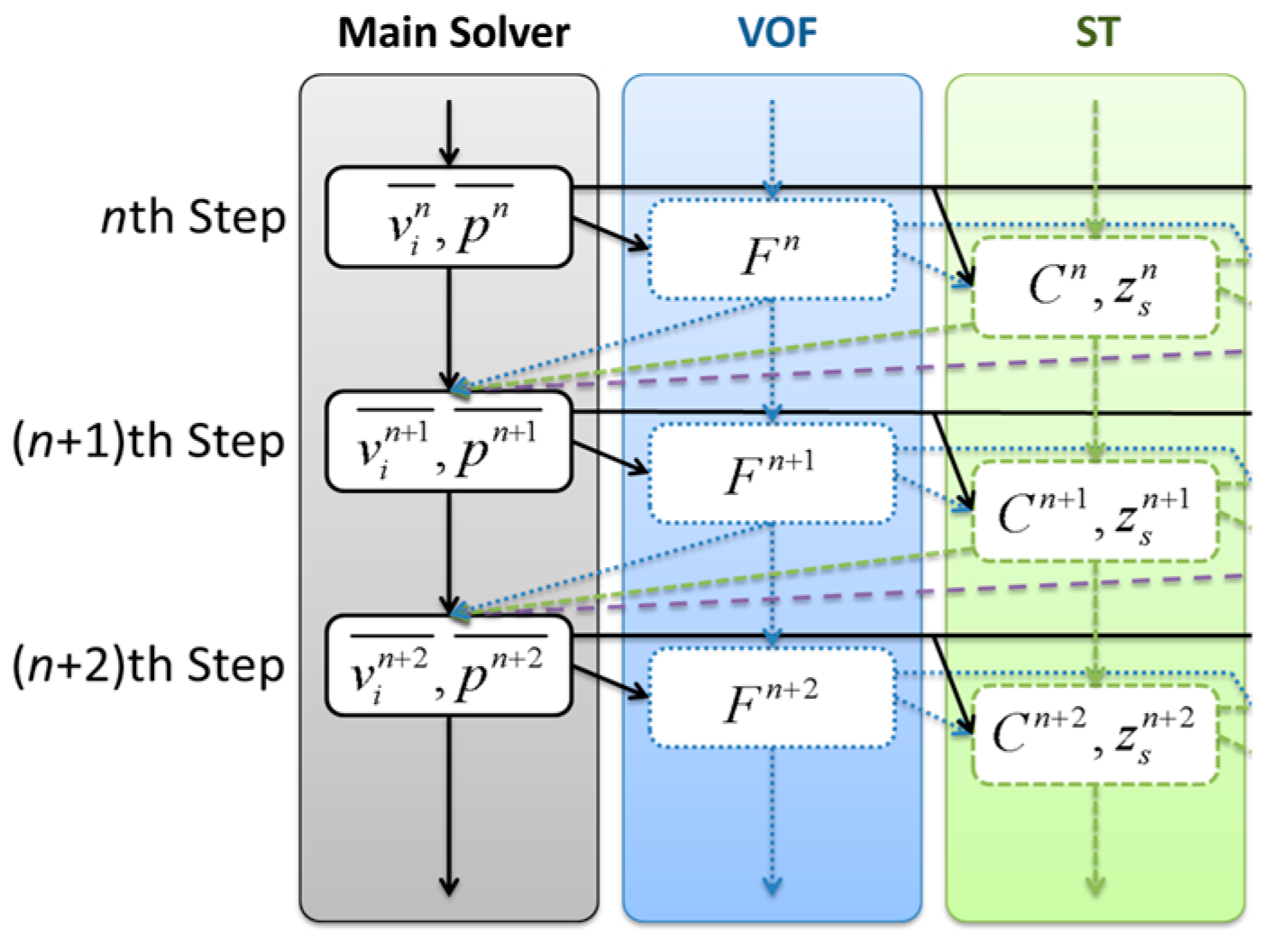
2.3. Coupling of Wave Field and Sediment Transport

The coupling in this study focused on integrating the wave field model with the sediment transport model. The procedure is as follows: (1) The main solver computes the velocity $\overline{v_i}$ (m/s) and pressure field $\overline{p}$ (Pa) within the seabed. (2) The VOF module is run using the data from the main solver to calculate the VOF. (3) The sediment transport module is executed using the values obtained from the VOF module to calculate the suspended sediment concentration C and the height of the moving bed surface $z_s$ (m). The calculation flowchart is shown in Figure 2.

To ensure computational efficiency, the sediment transport module, including the settling flux $q_j^S$, interacts dynamically with the hydrodynamic and morpho-dynamic processes within each computational time step. The settling velocity $w_{si}$ is calculated based on empirical formulations (e.g., Rubey’s equation) and integrated into the coupled framework. This integrated approach optimizes the interaction between modules, reducing the need for iterative recalculations and ensuring that sediment settling and transport processes are resolved concurrently within the coupled framework.

3. Model Validation

3.1. Experimental Case Set-Up

The geometry of the model was based on a wave flume. The experimental values were obtained from [1]. This experiment is a classic benchmark. For example, Yeganeh-Bakhtiary et al. [5] and Karagiannis et al. [25] used these experimental results to verify their work. Both studies demonstrate the utility of Xie’s dataset in benchmarking numerical models. However, the present model differs significantly from these approaches in its computational framework, sediment transport modeling, and model coupling methods. To support the numerical simulations conducted in this study, the wave flume used in the experiment is described as follows. The wave flume shown in Figure 3 is 38.0 m long, 0.80 m wide, and 0.6 m deep. A paddle-type wave generator is present at one end with a concrete vertical wall at the other end of the flume. The distance between the wave paddle and the wall is 32.9 m. A 6 m-long horizontal sand bed is formed in front of the wall, with a thickness of 0.15 m. A 1:30 slope is used to link the sand bed to the bottom of the flume. The water depths in the flume and above the flat sand bed are 0.45 m and 0.30 m, respectively.

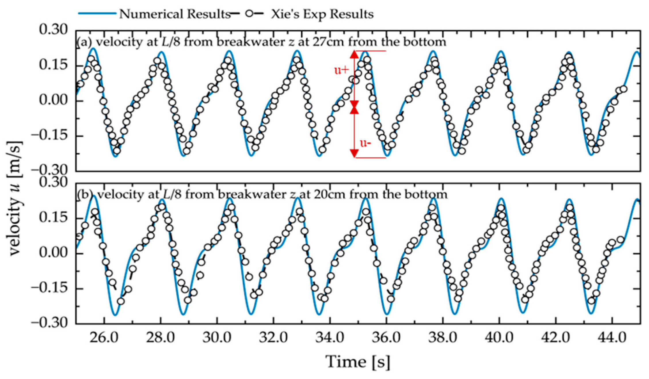
3.2. Wave Field Validation

In the experiment reported in [1], 26 tests were conducted with sand diameters exceeding 50% in size by weight, incident wave heights, and periods. The validation cases in this study focus on regular wave conditions, consistent with the experimental data reported by Xie [1]. The selected cases, No. 2a, No. 6a, and No. 25a, represent varying wave steepness, moderate (No. 2a), high (No. 6a), and low, with longer wave periods (No. 25a). These cases ensure robust validation of the model across diverse wave-induced sediment transport scenarios. While Xie’s dataset includes irregular wave tests, these were excluded due to their stochastic nature, requiring separate treatment. The chosen cases allow for precise validation under controlled conditions, providing a reliable basis for analyzing wave dynamics and sediment transport. The wave field validation section in this study considered the three cases summarized in

Table 1. Wave verification cases characteristics.

Case	H (cm)	T (s)	L (m)	H/L	$\mathit{H}/\mathit{g}{\mathit{T}}^2$
No. 2a	7.5	1.32	2.0	0.0375	0.0044
No. 6a	9.0	1.86	3.0	0.0300	0.0052
No. 25a	9.0	2.41	4.0	0.0125	0.0008

, where H is the wave height, T is the wave period, and L is the wavelength; $H/g{T}^2$ is defined as a dimensionless ratio in wave dynamics. These parameters provide a comprehensive baseline for understanding wave–seabed interactions and evaluating the model’s performance.

Numerical simulations were conducted using different configurations to assess the effects of the mesh resolution and damping zones on the wave behavior near the breakwater. The mesh resolutions, dx = 0.01 m and dx = 0.02 m, were not predetermined to be optimal; instead, they were selected based on prior studies, such as the work by Hou et al. [11]. These values provided an appropriate starting point for sensitivity analysis in this study. Moreover, two damping zone configurations were employed, damping_4L and damping_2L (L is the wavelength), which helped reduce wave reflection by dissipating excess energy near the boundaries. The number (4L or 2L) indicates the length of the damping zone, with 4L theoretically providing a more gradual dissipation than 2L.

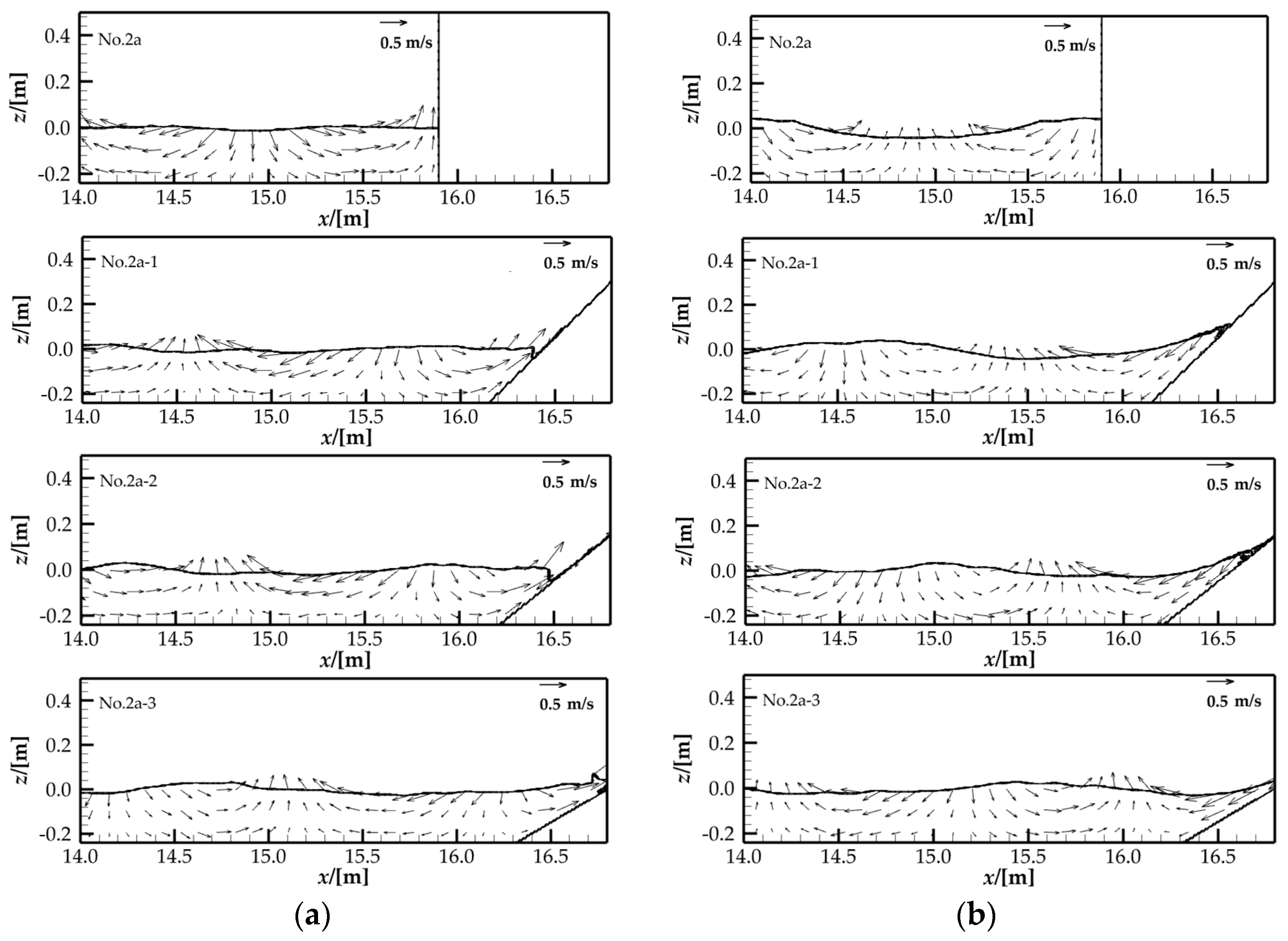
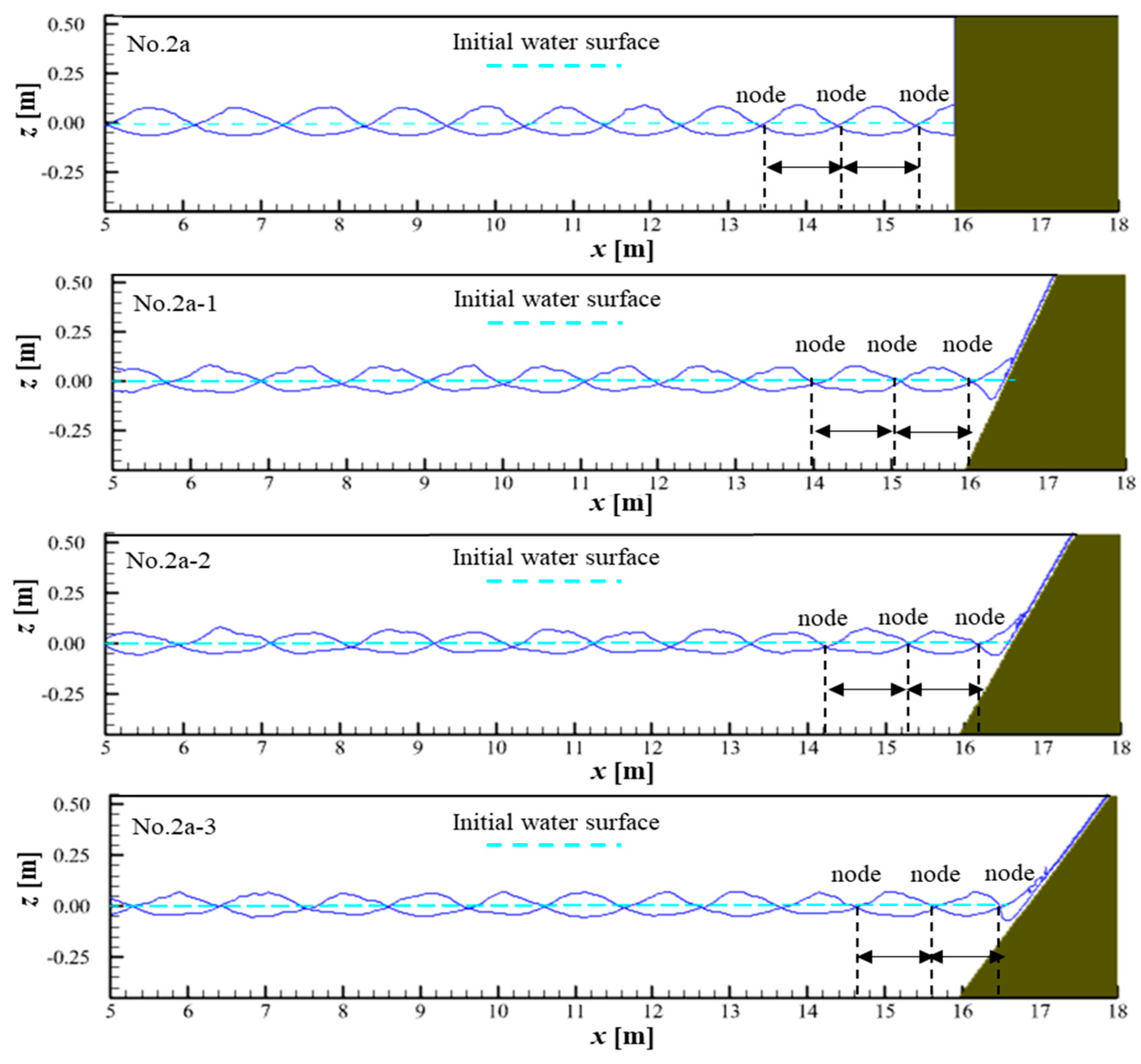
Hydrodynamic Results

Figure 4 shows a temporal change in water surface fluctuation 13.8 m and 1.0 m offshore of the breakwater for Case No. 2a. In particular, Figure 4a shows the wave profile at 13.8 m from the breakwater. During the first 10 s, the water surface remained stable, indicating that the incident wave did not reach this location. Over time, the incident wave approached, and the wave height gradually increased between 10 and 35 s. At approximately 35 s, the standing wave began to form and continued to develop, reaching its maximum height. The formation process required approximately 45 s, after which the wave height stabilized, and the standing wave maintained a steady amplitude. Figure 4b shows the wave profile at a location 1 m from the breakwater. At this position, owing to its proximity to the breakwater, wave reflection occurred rapidly, and the standing wave formed more quickly, reaching its peak at 40 s.

Figure 5 shows a comparison of the wave profiles for Case No. 2a for different damping zone configurations and mesh resolutions. In both cases, the numerical simulation results are compared for different damping zone configurations (damping_4L and damping_2L) and mesh resolutions (dx = 0.01 m and dx = 0.02 m), with experimental data from [1]. In Figure 5a, the surface elevation peaks vary slightly depending on the damping zone settings, with smaller mesh resolutions resulting in more pronounced peaks. The results in Figure 5b, obtained 1 m from the breakwater, show a similar trend, even though the waves settled into a more stable oscillation owing to their proximity to the reflective wall. Compared with the results in [1], both figures indicate a close match in the amplitude and frequency of the wave oscillations. The results demonstrate minimal differences between configurations, highlighting the robustness of the numerical model across various settings. Therefore, to save computing resources, we selected the damping zone (damping_2L) and mesh resolution (dx = 0.02 m) for the subsequent studies.

The velocity distribution is shown in Figure 6 at two different time instances and at a distance of one wavelength from the breakwater. Clear differences are observed between the wave crest and trough phases. In Figure 6a, the velocity vectors beneath the wave crest indicate an upward flow at the center and an outward horizontal flow on either side, reflecting the upward movement of water. In Figure 6b, at the wave trough, the flow reverses, with a downward motion at the center and inward flow from the sides, pulling water into the trough. These alternating flow patterns demonstrate the cyclical motion of water as the wave propagates. Upward and outward flows occurred during the crest, whereas downward and inward flows dominated during the trough, illustrating the complex fluid dynamics driving the wave energy transfer as it approached the breakwater.

Figure 7 shows a comparison between the numerical and the experimental wave profiles for Case No. 6a at two locations—(a) 12.9 m and (b) 1.5 m from the breakwater. From the results, at both 12.9 m and 1.5 m from the breakwater, a strong agreement between the numerical simulation (represented by the blue line) and the experimental data from [1] (represented by the dashed line) is observed. The wave profiles show a clear periodic pattern, and the numerical and experimental results demonstrate similar peak values and wave phases, even though slight amplitude discrepancies can be observed.

In addition to comparing the wave profile changes across different cases, we evaluated the velocity fields obtained from the experimental measurements and numerical simulations to comprehensively validate the performance of the model. Figure 8 shows the orbital velocity profiles for Case No. 25a at multiple depths. Specifically, Figure 8a shows the profile at x = 8/L from the breakwater, with measurements obtained at a depth of z = 27 cm above the bottom, whereas Figure 8b illustrates the profile at z = 20 cm from the bottom. The red arrows in Figure 8 highlight the positive and negative peak velocities, indicating the maximum number of oscillation points during each wave cycle. This visual representation illustrates the phase difference and the amplitude between the experimental and numerical results. In conclusion, for Case 25a, the comparison between the numerical simulations and the experimental data [1] showed a strong correlation in the velocity fields. The velocity profiles measured at a designated location from the bottom exhibit similar sinusoidal patterns. Although slight deviations were observed in the magnitudes of the positive and negative peak velocities, the general trend and phase were well captured.

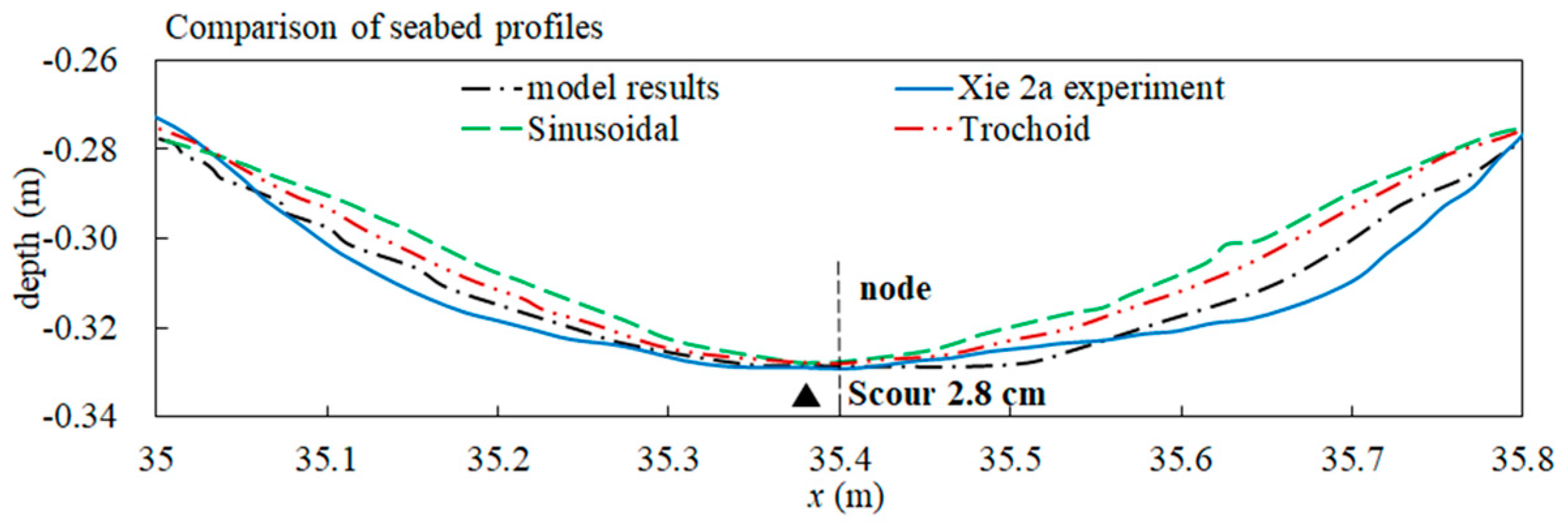
3.3. Seabed Profile Change Verification

In the sediment transport verification section, we focused on Case No. 2a, summarized in

Table 2. Sediment verification cases’ characteristics.

Case	${\mathit{D}}_{50}$	${\mathit{w}}_{\mathit{f}}$	H	d/L	Group
No. 2a	106 μm	0.7 cm/s	7.5 cm	0.15	Fine

, to ensure consistency and computational efficiency. This case was chosen because it represents moderate wave conditions (H = 7.5 cm, d/L = 0.15), which are well-suited for analyzing wave-induced scour and deposition. Additionally, by selecting one representative case, we ensure comparability between vertical and inclined breakwaters, which is a key focus of this study. While sediment transport simulations are computationally intensive due to the detailed seabed profile changes, the numerical methodology is robust and can be extended to other validated wave cases. In this case, $D_{50}$ is the median grain size, and $w_f$ is the sediment fall velocity.

3.3.1. Grid-Independence Analysis

A grid-independence test was conducted to determine the optimal grid resolution for sediment transport simulations. The tested z-direction grid resolutions included 0.0100 m, 0.0050 m, 0.0025 m, and 0.0010 m, while the x-direction resolution was fixed at 0.02 m, as summarized in

Table 3. Grid-independence analysis in z-direction.

Test	Grid Resolution in z-Direction (m)	Grid Resolution in x-Direction (m)
Grid 1	0.0100	0.02
Grid 2	0.0050	0.02
Grid 3	0.0025	0.02
Grid 4	0.0010	0.02

.

Figure 9 shows the seabed profile at various vertical grid resolutions at two time points. Between t = 140 s and t = 200 s, a notable evolution is observed in the seabed profile, with a more pronounced slope developing near the wall over time, especially in the finer grid cases. As the grid resolution is refined, a more detailed representation of the seabed morphology is observed. Finer grids provide smoother transitions and more precise representations of the sediment dynamics, ensuring accurate scouring depths and slope transitions. In contrast, coarser grids such as z = 0.0100 m and z = 0.0050 m introduce distortions, including overly smoothed slopes and under-represented scouring depths, which can affect the accuracy of sediment transport and seabed morphology predictions. Notably, z = 0.0025 m was selected as the optimal resolution because it captures sufficient detail while balancing computational efficiency. Finer grids, like z = 0.0010 m, require significantly higher computational costs due to the increased number of cells and iterations, while providing only marginal improvements in seabed profile accuracy.

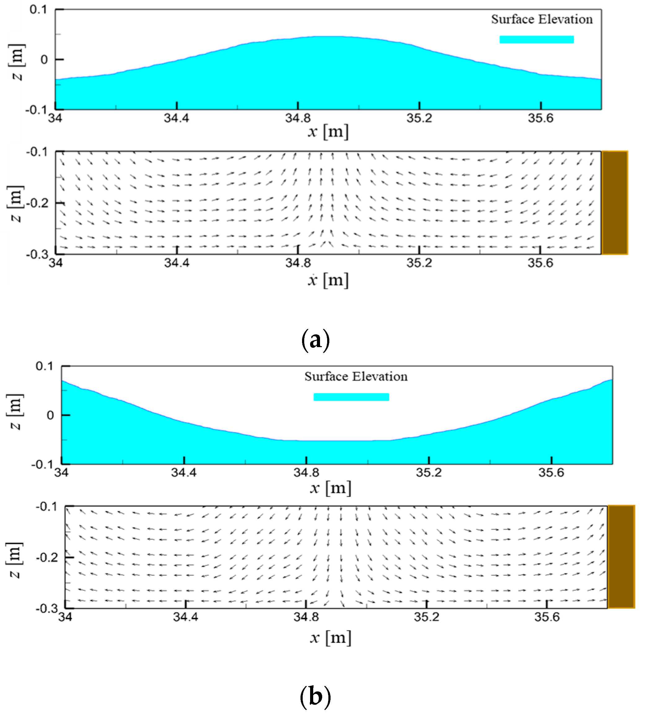
3.3.2. Morpho-Dynamic Results

Figure 10 shows the simulation results for breakwater scour over time. The results indicate that the seabed morphology changed. At t = 200 s, the sediment deposition is initially concentrated near the breakwater, with minimal changes observed offshore. This early stage of sediment accumulation shows a slight increase in the seabed close to the wall. At t = 400 s, distinct peaks and troughs begin to form near the breakwater, indicating that wave action results in sediment deposition in a patterned manner. As time progressed to t = 800 s, the seabed profile became more pronounced, and the height of the peaks and troughs near the breakwater increased. Sediment deposition near the wall reached higher levels, whereas offshore scour deepened further. Finally, at t = 1400 s, the morphological changes stabilized, and the sediment deposition near the breakwater reached a consistent height. The offshore scour remained well-defined and deeper, indicating continuous erosion in this region. These results demonstrate the dynamic interplay between sediment deposition and scouring, driven by wave-induced sediment transport.

Figure 11 shows the final numerical seabed profile, and the standing wave pattern shows a clear correlation between the sediment deposition and the wave dynamics. The antinode at x = 30.9 m aligns with the highest water surface oscillations, resulting in significant sediment deposition and peak formation on the seabed. In contrast, the nodes at x = 34.4 m and x = 35.4 m correspond to areas of minimal wave movement, where the sediment transport is lower, leading to troughs in the seabed. This pattern highlights the influence of the standing waves on the seabed morphology near the breakwater.

The comparison illustrated in Figure 12 highlights the effectiveness of the numerical model in replicating the experimental seabed profiles with remarkable accuracy. Both the numerical model (dashed black line) and the experimental data (solid blue line) show similar trends, capturing the essential node at x = 35.4 m with a scour depth of approximately 2.8 cm. This agreement confirms the reliability of the model, particularly in reproducing localized seabed deformation caused by wave-induced forces. To further validate the model’s performance, statistical parameters were employed. The RMSE (Root Mean Square Error) between the numerical and experimental profiles was computed as 0.00196 m, indicating minimal deviation. Furthermore, the R² (coefficient of determination) value of 0.0478 highlights a strong correlation between the model predictions and the experimental observations. This quantitative assessment reinforces the model’s robustness in accurately capturing wave-seabed interaction processes. However, the theoretical profiles, such as the sinusoidal and trochoidal curves, tend to overestimate the seabed elevation at the outer regions (e.g., x = 35.1 m and x = 35.7 m). These discrepancies arise because theoretical models are limited by their assumptions, neglecting complex wave–seabed interactions and nonlinear sediment transport processes. The close alignment of the numerical model with the experimental data demonstrates its ability to handle such complexities, making it a reliable tool for coastal and sediment engineering applications. Overall, the numerical model proves superior to theoretical approaches in capturing localized seabed deformations and wave-induced interactions.

4. Model Application

In the previous section, we demonstrated that our numerical model closely replicated both wave behavior and sediment dynamics, validating its effectiveness. Consequently, we applied the model to explore the effects of breakwater steepness on the wave and sediment interactions. The setup and configuration of this model are shown in Figure 13 and

Table 4. Numerical study of the breakwater steepness effects cases.

Case	d (m)	H (m)	L (m)	T (s)	${\mathit{D}}_{50}$ (μm)	Slope	Steepness
No. 2a	0.3	0.075	2.0	1.32	106	vertical	-
No. 2a-1	0.3	0.075	2.0	1.32	106	1:1.2	steep
No. 2a-2	0.3	0.075	2.0	1.32	106	1:1.5	steep
No. 2a-3	0.3	0.075	2.0	1.32	106	1:2.0	gentle

, respectively. The breakwater has a height of 1.0 m, with varying slope, as follows: vertical (Case No. 2a), 1:1.2 (Case No. 2a-1), 1:1.5 (Case No. 2a-2), and 1:2 (Case No. 2a-3). The water depth is 0.3 m, wave height is 0.075 m, and wave length is 2.0 m, with a wave period of 1.32 s. The median grain size is 106 μm. The wave characteristics, including a wave height of 0.075 m, wave period of 1.32 s, and wavelength of 2.0 m, were chosen to reflect realistic conditions commonly encountered in small-scale coastal engineering experiments. These parameters align with previous experimental setups, ensuring the comparability and validation of the numerical model. While this study focuses on specific wave conditions, the methodology is adaptable to a range of wave characteristics. Adjusting wave height, period, or slope conditions allows the model to analyze similar wave–sediment interactions, supporting its broader applicability.

4.1. Wave Characteristics in Different Breakwater Steepness

Figure 14 shows the results of free-surface motion and velocity vectors for standing waves across different breakwater steepness cases, including the vertical and sloped cases. In the vertical case (Case No. 2a), the strong wave reflection creates pronounced standing waves with sharp oscillations in the free surface and concentrated velocity vectors near the breakwater. This leads to a distinct wave profile with well-defined nodes and antinodes. As the breakwater slope changes from steep to gentle, the wave reflection is moderated, and the energy dispersion is more effective. In the steep slope case (Case No. 2a-1), while wave reflection is still noticeable, the slope dissipates the energy over a wider area, resulting in a more diffused velocity distribution. For gentler slopes (Case No. 2a-2 and Case No. 2a-3), wave reflections are further reduced, leading to smoother free surface transitions and a less pronounced standing wave effect. The velocity vectors become more evenly distributed, indicating greater energy dissipation along the slope. Overall, decreasing the steepness of the breakwater slope results in reduced wave reflection, improved energy dissipation, and a more uniform velocity distribution. This suggests that gentler slopes are effective in minimizing waves’ impact on coastal structures.

Figure 15 illustrates the free-surface profiles of standing waves across different breakwater steepness cases, demonstrating the intricate interaction between the wave reflection and slope design. In each case, the nodes (points of zero displacement) and antinodes (points of maximum amplitude) are clearly observed along the wave flume. The profiles represent the steady-state conditions achieved after the initial transient wave effects subsided, ensuring the stable periodic behavior of the nodes and antinodes. For a steep vertical breakwater (Case No. 2a), the nodes were positioned farther from the breakwater, with a larger distance between them, reflecting stronger wave reflection dynamics. As the slope became more gradual, the nodes moved closer to the structure, indicating that gentler slopes alter the wave reflection pattern by dispersing energy more evenly along the flume. This shift also affected the antinodes, aligning them closer to the structure as the slope decreased. The changes in the node and antinode positions illustrate the complex influence of the slope on energy dissipation, emphasizing the importance of carefully designing breakwaters to control the wave’s impact and reflection.

Overall, this pattern reveals the effects of slope steepness on energy dissipation and wave reflection, highlighting its importance in the design of effective coastal defense systems. The closer positioning of nodes with gentler slopes implies that these structures may absorb more energy within the flume, thereby influencing the wave behavior. Optimizing the breakwater design by considering slope steepness can improve coastal resilience and ensure a balance between wave reflection and energy dissipation.

4.2. Sediment Movement Characteristics in Different Breakwater Steepness

Figure 16 shows the evolution of the sediment seabed profiles under varying breakwater slopes at two different simulation times. Figure 16a shows the seabed profile at t = 125 s, which captures the early stages of sediment movement and scouring. Figure 16b shows the profile at t = 250 s, highlighting subsequent developments. The figures clearly show that sediment scour varies across different breakwater slopes. The results are observed for both t = 125 s and t = 250 s. The vertical breakwater Case No. 2a shows the most significant sediment displacement near the breakwater, with a pronounced scour depth reaching approximately 0.05 m at x = 15.5 m. As the breakwater slope becomes gentler in Cases No. 2a-1 (slope 1:1.2) and No. 2a-2 (slope 1:1.5), the scour depth slightly decreases, with the depths decreasing to approximately 0.045 m and 0.042 m, respectively. The gentlest slope configuration, Case No. 2a-3 (slope 1:2), exhibits the shallowest scour depth of approximately 0.035 m. In general, the results indicate that as the breakwater slope becomes gentler, the wave reflection and energy concentration near the base decrease, leading to less pronounced scour. Additionally, the wider scour areas observed with the gentler slopes suggest better wave energy dissipation, contributing to improved sediment stability. The reduced reflection of energy helps mitigate sediment displacement, with the deposition zones stabilizing more effectively in gentle slope configurations.

5. Conclusions

A numerical approach was proposed in this study, which included three primary components: the main solver, the VOF solver, and the sediment transport module. The main solver computes the velocity and pressure fields in the seabed region, whereas the VOF module tracks the free surface by using the computed flow fields. The ST module calculates the suspended sediment concentrations and bed morphology changes based on the VOF results.

The model was first validated against experimental results, showing strong agreement in simulating the wave motion and sediment transport capabilities. The model can effectively capture wave patterns, including standing waves and the corresponding sediment erosion and deposition.

After the validation, the model was applied to various breakwater slopes to obtain significant insights. For example, the results showed that steeper breaker slopes led to more concentrated wave energy near the structure, resulting in deeper scouring and higher sediment displacement. In contrast, gentler slopes provided improved energy dissipation, resulting in reduced sediment scour and a wider deposition area, indicating that gentle slopes can help improve sediment stability by reducing wave reflection and enhancing energy absorption.

In conclusion, these results demonstrate the versatility of the model in validating physical experiments and providing insights into sediment transport under different structural configurations, and may offer practical guidance for optimizing breakwater design in the future. However, this study is limited to a two-dimensional simulation, restricting its ability to replicate the effects of complex three-dimensional wave actions on shoreline structures. Additionally, while the numerical model was validated by comparing seabed profile changes, it lacks direct comparisons of sediment transport metrics (e.g., rate, quantity, direction) with experimental data. The quantitative validation of these parameters is essential for enhancing the model’s accuracy, and should be further addressed in future research.

Future work could extend the numerical model to simulate irregular wave conditions, incorporating advanced wave generation techniques and stochastic sediment transport processes. This would enable the model to replicate the transient wave group effects and complex sediment dynamics observed in the experiments by Daloui and Jamali [26], including hysteresis effects and cohesive sediment behavior. Such enhancements would broaden the model’s applicability to real-world coastal environments where irregular wave conditions dominate.

References

1. Xie, S.L. Scouring Patterns in Front of Vertical Breakwaters and Their Influences on the Stability of the Foundations of the Breakwaters; Delft University of Technology: Delft, The Netherlands, 1981. [Google Scholar]
2. Li, Z.; Jeng, D.S. Dynamic soil response around two-layered detached breakwaters: Three-dimensional OpenFOAM model. Ocean Eng. 2023, 268, 113582. [Google Scholar] [CrossRef]
3. Sumer, B.; Fredsoe, J. The Mechanics of Scour in the Marine Environment; World Scientific: River Edge, NJ, USA, 2002. [Google Scholar]
4. Hajivalie, F.; Yeganeh-Bakhtiary, A.; Houshanghi, H.; Gotoh, H. Euler–Lagrange model for scour in front of vertical breakwater. Appl. Ocean Res. 2012, 34, 96–106. [Google Scholar] [CrossRef]
5. Yeganeh-Bakhtiary, A.; Houshangi, H.; Abolfathi, S. Lagrangian two-phase flow modeling of scour in front of vertical breakwater. Coast. Eng. J. 2020, 62, 252–266. [Google Scholar] [CrossRef]
6. Chauchat, J.; Cheng, Z.; Nagel, T.; Bonamy, C.; Hsu, T.J. SedFoam-2.0: A 3-D two-phase flow numerical model for sediment transport. Geosci. Model Dev. 2017, 10, 4367–4392. [Google Scholar] [CrossRef]
7. Li, J.; Chen, X. A multi-dimensional two-phase mixture model for intense sediment transport in sheet flow and around pipeline. Phys. Fluids 2022, 34, 103314. [Google Scholar] [CrossRef]
8. Meyer-Peter, E.; Müller, R. Formulas for Bed-load Transport; IAHR: Madrid, Spain, 1948. [Google Scholar]
9. Rouse, H. Modern conceptions of the mechanics of fluid turbulence. Trans. Am. Soc. Civil Eng. 1937, 102, 463–505. [Google Scholar] [CrossRef]
10. Engelund, F.; Hansen, E. A Monograph on Sediment Transport in Alluvial Streams; Technical University of Denmark Oservoldgade 10: Copenhagen K.; Delft University of Technology: Delft, The Netherlands, 1967; Available online: http://resolver.tudelft.nl/uuid:81101b08-04b5-4082-9121-861949c336c9 (accessed on 18 November 2024).
11. Hou, Y.; Nakamura, T.; Cho, Y.H.; Mizutani, N.; Tomita, T. Influence of tsunami-driven shipping containers’ layout on their motion. J. Mar. Sci. Eng. 2022, 10, 1911. [Google Scholar] [CrossRef]
12. Nakamura, T.; Yim, S.C. Development of a 3D numerical model considering interactions between wave fields and topographical changes and its application to erosion and scouring phenomena. Proc. Civil Eng. Ocean JSCE 2009, 25, 1227–1232. [Google Scholar]
13. Mizutani, N.; Maeda, K.; Ayman, M.; Mostafa, G.; McDougal, W. Evaluation of resistance coefficient of permeable structures and numerical analysis of nonlinear interaction between waves and submersible permeable structures. Proc. Coast. Eng. JSCE 1996, 43, 131–135. [Google Scholar] [CrossRef]
14. Brackbill, J.U.; Kothe, B.D.; Zemach, C. A continuum method for modeling surface tension. J. Comp. Phys. 1992, 100, 335–354. [Google Scholar] [CrossRef]
15. Kobayashi, H. The subgrid-scale models based on coherent structures for rotating homogeneous turbulence and turbulent channel flow. Phys. Fluids. 2005, 17, 045104. [Google Scholar] [CrossRef]
16. Iwata, K.; Kawasaki, H.; Kin, D. Numerical analysis of wave breaking by underwater structures. J. Coast. Eng. 1995, 42, 781–785. [Google Scholar]
17. Roulund, A.; Sumer, B.M.; Fredsøe, J.; Michelsen, J. Numerical and experimental investigation of flow and scour around a circular pile. J. Fluid Mech. 2005, 534, 351–401. [Google Scholar] [CrossRef]
18. Engelund, F.; Fredsøe, J. A sediment transport model for straight alluvial channels. Hydrol. Res. 1976, 7, 293–306. [Google Scholar] [CrossRef]
19. Iwagaki, Y. Hydraulic study of critical tractive force. Proc. Trans. Japan Soc. Civil Eng. 1956, 41, 1–21. [Google Scholar] [CrossRef]
20. Nielsen, P.; Svendsen, I.A.; Staub, C. Onshore-offshore sediment movement on a beach. Proc. Int. Conf. Coast. Eng. ASCE 1978, 16, 1475–1492. [Google Scholar] [CrossRef]
21. Nielsen, P. Coastal Bottom Boundary Layers and Sediment Transport; World Scientific: River Edge, NJ, USA, 1992. [Google Scholar]
22. Allen, J.R.L. Principles of Physical Sedimentology; Allen and Unwin: Crows Nest, Australia, 1985; p. 272. [Google Scholar]
23. Miyamoto, J.; Sasa, M.; Tokuyama, R.; Sekiguchi, H. Observation of gravity flow and solidification/sedimentation processes of underwater sediments. Proc. Coast. Eng. JSCE 2004, 51, 401–405. [Google Scholar] [CrossRef]
24. Nakamura, T.; Cho, Y.; Mizutani, N. A consideration on the treatment of slope failures when calculating topographical changes due to sand drift. In Proceedings of the 71st Annual Conference Japanese Society Civil Engineering, Sendai, Japan, 7–9 September 2016; pp. 437–438. [Google Scholar]
25. Karagiannis, N.; Karambas, T.; Koutitas, C. Numerical simulation of scour depth and scour patterns in front of vertical-wall breakwaters using OpenFOAM. J. Mar. Sci. Eng. 2020, 8, 836. [Google Scholar] [CrossRef]
26. Daloui, A.; Jamali, M. Experimental Study of Scour Due to Breaking Waves in Front of Vertical-Wall Breakwaters. In Proceedings of the ASME 2004 23rd International Conference on Offshore Mechanics and Arctic Engineering, Vancouver, BC, Canada, 20–25 June 2004. [Google Scholar] [CrossRef]
Figure 1. Forces acting on a sediment particle in bedload transport on a sloping bed.
Jmse 12 02261 g001
Figure 2. Calculation flowchart of the developed model.
Jmse 12 02261 g002
Figure 3. Wave flume used for validation.
Jmse 12 02261 g003
Figure 4. Numerical wave profiles of Case No. 2a: (a) 13.8 m from the breakwater just before the slope; (b) 1.0 m from the breakwater.
Jmse 12 02261 g004
Figure 5. Numerical comparison between different damping zones and mesh resolution wave profiles of Case No. 2a: (a) 13.8 m from the breakwater just before the slope; (b) 1.0 m from the breakwater.
Jmse 12 02261 g005
Figure 6. Surface elevation and particle velocity distribution of Case No. 2a at different times: (a) velocity distribution beneath the wave crest; (b) velocity distribution beneath the wave trough.
Jmse 12 02261 g006
Figure 7. Numerical comparison between the experimental and numerical wave profiles of Case No. 6a: (a) 12.9 m from the breakwater just before the slope; (b) 1.5 m from the breakwater.
Jmse 12 02261 g007
Figure 8. Orbital velocity profiles of test Case No. 25a: (a) velocity at x = 8/L from breakwater, z = 27 cm from the bottom; (b) velocity at x = 8/L from breakwater, z = 20 cm from the bottom.
Jmse 12 02261 g008
Figure 9. Seabed profile evolution at various vertical grid resolutions at two time points: (a) t = 140 s; (b) t = 200 s.
Jmse 12 02261 g009
Figure 10. Simulation results for sediment movement near breakwater over time: (a) t = 200 s; (b) t = 400 s; (c) t = 800 s; (d) t = 1400 s.
Jmse 12 02261 g010
Figure 11. Final numerical seabed profile and standing wave pattern.
Jmse 12 02261 g011
Figure 12. Comparison between the model results and experimental and theoretical data of the seabed profiles and scouring depth at the final point (t = 1400 s).
Jmse 12 02261 g012
Figure 13. Numerical study of the breakwater steepness effects cases setup.
Jmse 12 02261 g013
Figure 14. Free surface motion and velocity vectors for standing waves across different breakwater steepness cases: (a) as waves advance towards the breakwater; (b) as waves are reflected from the breakwater.
Jmse 12 02261 g014
Figure 15. Free surface profile of the standing wave in different breakwater steepness cases.
Jmse 12 02261 g015
Figure 16. Evolution of sediment seabed profiles under varying breakwater slopes at two different simulation times: seabed profiles at (a) t = 125 s; (b) t = 250 s.
Jmse 12 02261 g016