Global Mean Sea Level Change Projections up to 2100 Using a Weighted Singular Spectrum Analysis

Abstract

This paper forecasts global mean sea level (GMSL) changes from 2024 to 2100 using weighted singular spectrum analysis (SSA) that considers the formal errors of the previous GMSL time series. The simulation experiments are first carried out to evaluate the performance of the weighted and traditional SSA approaches for GMSL change prediction with two evaluation indices, the root mean square error (RMSE) and mean absolute error (MAE). The results show that all the RMSEs and MAEs of the weighted SSA are smaller than those of the traditional SSA, indicating that the weighed SSA can predict GMSL changes more accurately than the traditional SSA. The real GMSL change rate derived from weighted SSA is approximately 1.70 ± 0.02 mm/year for 1880–2023, and the predicted GMSL changes with the first two reconstructed components reaches 796.75 ± 55.92 mm by 2100, larger than the 705.25 ± 53.73 mm predicted with traditional SSA, with respect to the baseline from 1995 to 2014. According to the sixth Assessment Report of Intergovernmental Panel on Climate Change (IPCC AR6), the GMSL change by 2100 is 830.0 ± 152.42 mm/year with the high-emission scenarios is closer to weighted SSA than traditional SSA, though SSA predictions are within the prediction range of IPCC AR6. Therefore, the weighted SSA can provide an alternative future GMSL rise prediction.

1. Introduction

Sea level rise is considered one of the significant climate change components that may affect storminess, precipitation, temperature and the health of functionally linked neighboring ecosystems [1,2,3,4,5,6]. The mean sea level is predicted to increase by 30–100 cm by 2100, according to the Intergovernmental Panel on Climate Change (IPCC) Special Report on Emissions Scenarios [7,8]. Statistics show that approximately 200 countries and regions around the world lie along coastal areas or in the ocean, including North Europe, Japan, America, China and India. Thus, rising sea levels may result in the submergence of islands and changes in microclimates [9], negatively impacting coastal economies and habitat migration [10].

Sea level rise forecasting is essential for producing future development and planning strategies and mitigating the severe consequences of such a rise. The prediction errors of a global sea level rise by 2100 are large and deserve to be reduced. Typically, quantitative sea level rise prediction is executed with the assumption that one can use past information about the variable being forecast and assume that the pattern of the past data will continue. Several previous studies have explored dynamic models for sea level rise prediction or statistical models based on climate-related predictors [11] for sea level forecasting. The Intergovernmental Panel on Climate Change [12] projected that the sea level would reach 0.18–0.59 m above the present mark by the end of the 21st century. Still, an ice flow dynamics calving estimate was lacking. Calving was added by Pfeffer et al. [13], who reported an SLR of 0.8–2.0 m by 2100. Rahmstorf [14], who used a semi-empirical method that linked temperature changes with observed sea level rise to assess future global mean sea level change, indicated that the SLR will reach 0.5–1.4 m by the end of the 21st century. The IPCC used a climate model to predict that the global average sea level will increase by 0.26–0.82 m [12] by 2081–2100 compared to the level observed from 1986 to 2005.

However, due to the complexity of the driving mechanism of sea level changes and the extreme sensitivity of dynamic models to their key parameters, there is a considerable difference between the results predicted by the existing dynamic models and the measured data. Therefore, some scholars have questioned these prediction results [14,15,16]. Although satellite altimeter data are highly accurate, time series containing altimeter data are relatively short, and sea level data before the 1990s are missing. At present, these time series cannot play a better role in the study and prediction of long-term sea level change trends. Therefore, we use the merged global mean sea level (GMSL) change series from 1880 to 2023 with the GMSL change product from Church and White [17] and the GSFC [18] derived from altimetry datasets.

Adopting suitable time series analysis methods is essential for analyzing previous GMSL time series and forecasting future GMSL changes. A meaningful decomposition of the input GMSL time series into its signal and noise components leads to a better understanding of the sea level change process, especially for the more accurate forecasting of future sea levels. According to the relevant literature, many methods and models, such as singular spectrum analysis (SSA) [19], climate models [7] and semi-empirical models [14,16,20], and autoregressive and prophet models [21], have been used to analyze and forecast sea level rises. Compared to other methods, SSA can extract long-term trends and periodic components and forecast GMSL increases [19,22].

Considering that the accuracies of the GMSL change series are not equal, Wang et al. [23] proposed a new singular spectrum analysis (SSA) approach with stabilizing weights by taking the formal errors into account; the weight of time series data is constructed based on the ratio of the formal error to the signal power spectrum of a time series, whose weighted approach changes the signal structure to some extent. Considering that the formal errors are related to the observation error but not necessarily related to the signal on the basis that signals are independent of noise, Li and Shen [24] developed an improved principal component analysis by just weighting the noise term so as to ensure the signal structure is not destroyed. Shen et al. [25] extended the weighted approach to multichannel SSA (MSSA) to develop a new weighted MSSA and successfully applied it to extract the geophysical signals from noisy Gravity Recovery and Climate Experiment (GRACE) spherical harmonics solutions. In this study, we simplify the weighted MSSA to develop a weighted SSA approach, which keeps the signals fixed when extracting GMSL signals and forecasting future GMSL changes. The remainder of this paper is organized as follows. The weighted SSA approach is introduced after the traditional SSA process and is briefly presented in Section 2. The results and analysis are presented in Section 3, and conclusions are given in Section 4.

2. Methods and Employed Datasets

2.1. Weighted Singular Spectrum Analysis

For a time series $x_i(1\le i\le N)$, we can construct an $L\times K,K=N-L+1$ trajectory matrix $\mathit{X}$ with a window length L [26].

$$\mathit{X}=\left[\begin{array}{cccccc}{x}_1& x_2& \cdots & x_{i+1}& \cdots & x_{N-L+1}\\ x_2& x_3& \cdots & x_{i+2}& \cdots & x_{N-L+2}\\ ⋮& ⋮& ⋮& ⋮& ⋮& ⋮\\ x_L& x_{L+1}& \cdots & x_{i+L}& \cdots & x_N\end{array}\right]$$

(1)

Set the lagged covariance matrix $C=X{X}^{\mathrm{T}}$; then, $C$ is decomposed as $C=V\Lambda V^{\mathrm{T}}$, and $\Lambda$ is a diagonal matrix with eigenvalues (${\lambda }_k$) as its diagonal elements sorted in descending order. The row vectors of the orthogonal matrix $V$ are the eigenvectors $v_k$. The principal component matrix $A$ is given by $A=VX$. And the kth row vector of $A$($a_k$) is called the $k\mathrm{th}$ Principle Components (PCs). Its ith element ($a_{k,i}$) is computed with

$$a_{k,i}={\displaystyle \sum _{j=1}^L{x}_{i+j-1}{v}_{k,j}},1\le i\le N-L+1$$

(2)

where $v_{k,j}$ is the jth element of $v_k$. The kth reconstructed components (RCs) of the time series with the kth PCs as [26]

$$x_i^k=\left\{\begin{array}{ll}{\displaystyle \frac{1}{i}}{\displaystyle \sum _{j=1}^i{a}_{k,i-j+1}{v}_{k,j}}& 1\le i\le L-1\\ {\displaystyle \frac{1}{L}}{\displaystyle \sum _{j=1}^L{a}_{k,i-j+1}{v}_{k,j}}& L\le i\le N-L+1\\ {\displaystyle \frac{1}{N-i+1}}{\displaystyle \sum _{j=i-N+L}^L{a}_{k,i-j+1}{v}_{k,j}}& N-L+2\le i\le N\end{array}\right.$$

(3)

Since the variances of RCs, i.e., eigenvalues of covariance, are sorted in descending order, the first several RCs contain most time series signals. In contrast, the remaining RCs can be treated as noise. Thus, the signal ($s$) is reconstructed with the first n RCs.

$$s_i={\displaystyle \sum _{k=1}^n{x}_i^k},i=1,2,\cdots ,N$$

(4)

where $s_i$ denotes the ith element of reconstructed signals from n-dominant RCs.

The SSA commonly uses Equations (1)–(4) to process a time series without using its covariance information, which implies that the observational noise of the time series is treated as white noise. Therefore, it is not reasonable to deal with the time series with an equal unit weight in formulating the lagged covariance $C=X{X}^{\mathrm{T}}$.

The formal errors are related to the noise term but not correlated with the signal [24,25]. Usually, a time series $x_i(1\le i\le N)$ can be represented with signal $s_i$ and noise $e_i$ as follows:

$$x_i=s_i+e_i$$

(5)

To directly use Equations (2) and (3) to form lagged covariance, the time series is generated as follows:

$$x_i^{\prime }=s_i+{\displaystyle \frac{{\sigma }_0}{{\sigma }_i}}{e}_i$$

(6)

where $s_i$ and $e_i$ have the same meaning as in Equation (5); ${\sigma }_i$ represents the formal error of the ith epoch; and ${\sigma }_0$ is the standard deviation of the unit weight of the time series, which is calculated with the principle of keeping the sum of the weight equal to the length (N) of the time series:

$${\displaystyle \sum P_i}={\displaystyle \sum {\sigma }_0^2/{\sigma }_i^2}=N$$

(7)

where $P_i$ is the weight of the ith epoch. Then, we can derive the standard deviation of the unit weight as follows:

$${\sigma }_0=\sqrt{\mathrm{N}/{\displaystyle \sum 1/{\sigma }_i^2}}$$

(8)

If ${\sigma }_0$ is determined, the weight scale ${\sigma }_0/{\sigma }_i$ in Equation (8) is obtained. The priori values of $s_i$ and $e_i$ in Equation (6) are determined by traditional SSA. Then, we can derive the standard deviation $\sigma$ of Equation (8) and update the newly generated time series based on Equation (6) and iteratively extract the signal until its difference $\Delta {\widehat{s}}_i$ between two adjacent iterations satisfies the threshold

$$\left|\Delta {\widehat{s}}_i\right|<{10}^{-2}\mathrm{mm}$$

(9)

The new proposed sea level rise prediction approach, which takes formal errors into account, is called weighted singular spectrum analysis (SSA). To test the performance of weighted SSA, we make comparisons with traditional SSA in this study. Note that, in fact, the weighted SSA is the simplified version of the weighted multi-channel SSA approach [25], and for homogeneous time series, it has the same formal error for all epochs; thus, the weight factor is equal to 1 and Equation (6) reduces to Equation (5), and the weighted SSA is equivalent to the traditional SSA at this point.

In this study, we use the linear recurrent forecasting method with weighted SSA to predict the GMSL change for the future. The theory is introduced briefly as follows:

Let I be the chosen set of eigentriples, $P_i\in R^L,i\in I$ be the corresponding eigenvectors, $\underset{¯}{P_i}$ be their first L-1 coordinates, ${\pi }_i$ be the last coordinate of $P_i$, and $v^2={\displaystyle {\sum }_{i\in I}{\pi }_i^2}$ be the series reconstructed by I. Define $R={(a_{L-1},\cdots ,a_1)}^{\mathrm{T}}$ as

$$R={\displaystyle \frac{1}{1-v^2}}{\displaystyle \sum _{i\in I}{\pi }_i\underset{¯}{P_i}}$$

(10)

The recurrent forecasting algorithm can be formulated as follows:

(1)

The time series $Y_{N+M}=(y_1,\cdots ,y_{N+M})$ is defined by

$$y_i=\left\{\begin{array}{ll}{\tilde{x}}_i& i=1,\cdots ,N\\ {\displaystyle \sum _{j=1}^{L-1}{a}_j{y}_{i-j}}& i=N+1,\cdots ,N+M\end{array}\right.$$

(11)

(2)

The numbers $y_{N+1},\cdots ,y_{N+M}$ form the M terms of the recurrent forecast. Thus, recurrent forecasting is performed using the linear recurrence relation with coefficients $\{a_j,j=1,\cdots ,L-1\}$.

After forecasting the future GMSL rise, the accuracy of a forecast needs to be estimated. Here, we apply the Monte Carlo algorithm [27] to obtain 95% confidence intervals for traditional and weighted SSA.

2.2. Evaulation Indices

The simulation experiments and real global mean sea level change series are analyzed in this study. For the simulation experiments, to evaluate the prediction accuracy of the weighted SSA approach relative to the weighted SSA method, the indices of root mean square error (RMSE) and mean absolute error (MAE) are used. RMSE is calculated by using the differences between the real and predicted GMSL signals as follows:

$$\mathrm{RMSE}=\sqrt{{\displaystyle \frac{1}{N}}{\displaystyle \sum _{i=1}^N{(s_i-{\widehat{x}}_i)}^2}}$$

(12)

where ${\widehat{x}}_i$ denotes the GMSL signal predicted for the ith epoch via the weighted SSA and traditional SSA and $s_i$ is the real GMSL signal at the ith epoch. The mean absolute error (MAE) is calculated as

$$\mathrm{MAE}={\displaystyle \frac{1}{N}}{\displaystyle \sum _{i=1}^N\left|s_i-{\widehat{s}}_i\right|}$$

(13)

2.3. Employed Datasets

In this study, we use the monthly sea-level reconstruction product from Church and White [17], who also provided an estimate of the formal error induced by global mean sea-level change estimates from January 1880 to December 2013. The GMSL time series was corrected for glacial isostatic adjustment (GIA) [28], but an inverted barometer correction was not applied. In the state-space approach, these formal errors (measured as standard deviations) are directly used to parameterize the time-varying variances of the measurement errors yielded by the sea-level time series. The monthly GMSL time series derived from tide gauge records is downloaded from the website (http://www.cmar.csiro.au/sealevel/sl_data_cmar.html, accessed on 20 May 2024). For the period from 2014 to 2023, the GMSL changes were computed at the NASA Goddard Space Flight Center under the auspices of the NASA Sea Level Change program, and the change data were generated using the Integrated Multi-Mission Ocean Altimeter Datasets (http://podaac.jpl.nasa.gov/dataset/MERGED_TP_J1_OSTM_OST_ALL_V51, accessed on 20 May 2024). Then, the merged GMSL change series from 1880 to 2023 were obtained based on the overlapping period from 1993 to 2013. The IPCC AR6 sea-level rise projections dataset under the high-emission scenarios (SSP5-8.5) with medium confidence was accessed at https://podaac.jpl.nasa.gov/announcements/2021-08-09-Sea-level-projections-from-the-IPCC-6th-Assessment-Report (accessed on 20 May 2024) [29].

3. Results and Analysis

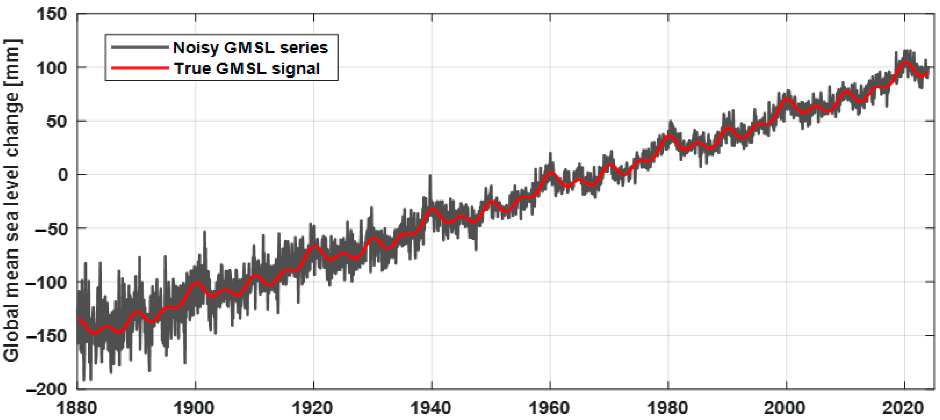
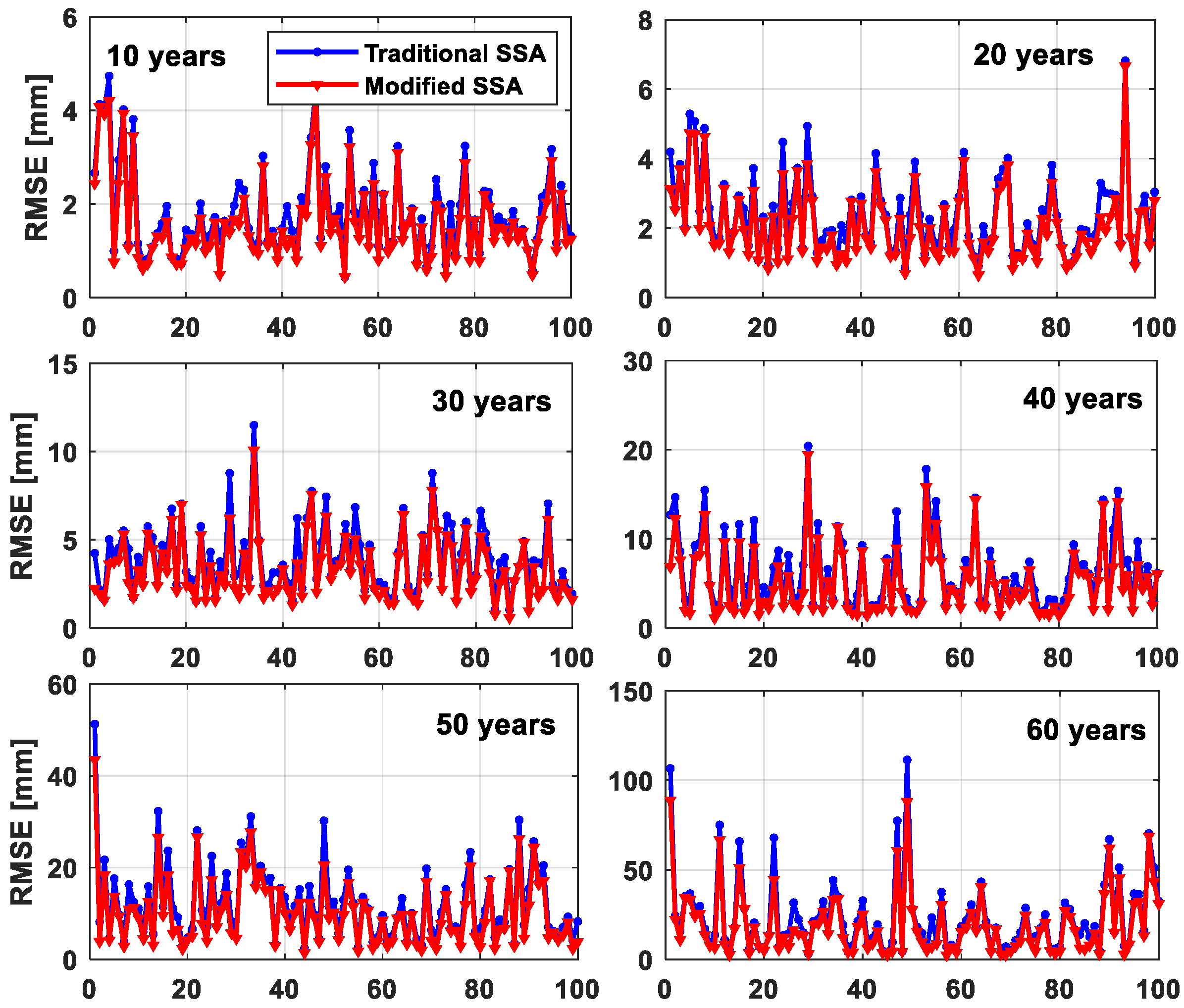
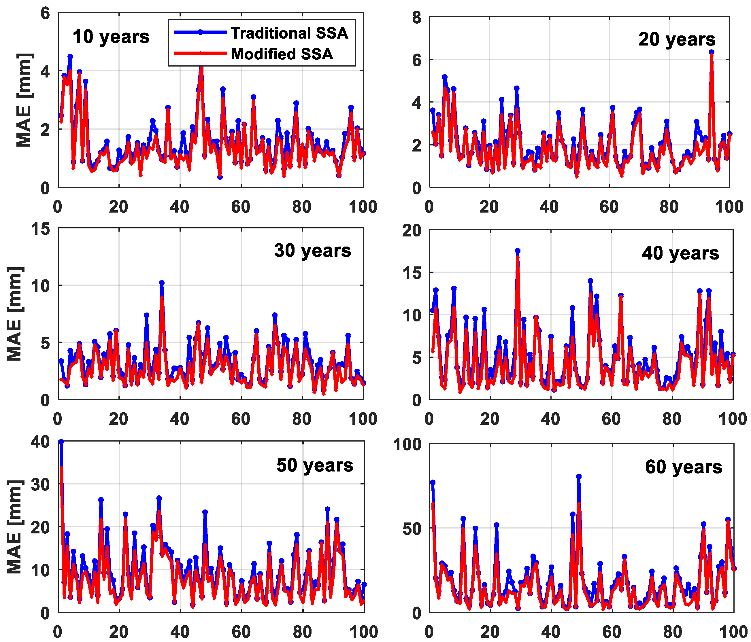
3.1. Prediction of Global Mean Sea Level Changes with Simulation Cases

To demonstrate the performances of the weighted SSA and traditional SSA methods in forecasting GMSL changes, we simulate the monthly GMSL change series with linear trend, periodic, and noise terms. From 1880 to 2023, the simulated global sea level increase rate was 1.70 mm/year. The simulated periodic components ($c(t)$) include five-year, ten-year, and twenty-year signals. The corresponding uncertainty series derived from the real permanent service for mean sea level (PSMSL) (http://www.psmsl.org, accessed on 20 May 2024) is adopted. Then, we simulate noise series $e(t)$ with zero means but different standard deviations according to the uncertainty series obtained in different epochs. Specifically, a synthetic time series is expressed as

$$x(t)=y(t)+c(t)+e(t)$$

(14)

where $y(t)$ is the long-term trend (Equation (15)); $c(t)$ is the periodic signal (see Equation (16)); and the unit of $t$ is months.

$$y(t)=-150+1.7/12\times t,t=1,2,\cdots ,N$$

(15)

$$c(t)=5\cos ({\omega }_{1}t)+5\cos ({\omega }_{2}t)+5\cos ({\omega }_{3}t)$$

(16)

where ${\omega }_1=2\pi /60$, ${\omega }_2=2\pi /120$ and ${\omega }_3=2\pi /240$.

The simulated GMSL change series and the true signals are presented in Figure 1, which includes 1728 monthly averaged data points spanning from 1880 to 2023. For the simulation cases, we select 480 as the window length and 8 as the reconstruction order.

Figure 2 shows the GMSL change series predicted by the weighted and traditional SSA approaches for lengths ranging from 10 years to 60 years with a step size of 10 years. With an increasing prediction length, the prediction error and uncertainty increase.

Table 1. The RMSEs and MAEs of weighted SSA and traditional SSA approaches for different prediction lengths.

Prediction Length [Years]	RMSE/mm		MAE/mm
	Traditional SSA	Weighted SSA	Traditional SSA	Weighted SSA
10	1.96	1.64	1.58	1.37
20	2.58	2.07	2.37	1.90
30	4.48	2.54	3.62	2.00
40	6.80	4.25	5.52	3.38
50	10.72	7.81	8.94	6.42
60	19.13	12.10	14.65	8.83

presents the RMSEs and MAEs computed for the weighted SSA and traditional SSA methods for the six prediction cases. It is obvious that all the RMSEs and MAEs of the weighted SSA are smaller than those of the traditional SSA, indicating that the weighted SSA can better forecast GMSL changes than the traditional SSA due to its consideration of formal errors. In addition, as the prediction length increases, the RMSE and MAE increase.

To demonstrate the reliability and advantages of the weighted SSA relative to the traditional SSA, 100 simulations are carried out with the synthetic time series generated by Equation (1). The RMSEs and MAEs produced over 100 simulations with different prediction lengths, which are shown in Figure 3 and Figure 4. All the RMSEs and MAEs of the weighted SSA are smaller than those of the traditional SSA, similar to the results in Table 1. The mean RMSEs and MAEs produced by the traditional SSA and weighted SSA for 100 simulations are presented in

Table 2. The mean RMSEs and MAEs of 100 simulations by weighted SSA and traditional SSA approaches.

Prediction Length [Years]	RMSE/mm			MAE/mm
	Traditional SSA	Weighted SSA	IMP/%	Traditional SSA	Weighted SSA	IMP/%
10	1.80	1.59	11.67	1.59	1.40	11.95
20	2.36	2.07	12.29	2.02	1.77	12.38
30	3.94	3.30	16.24	3.28	2.74	16.46
40	6.18	5.05	18.28	5.11	4.18	18.20
50	12.20	10.08	17.38	9.82	8.12	17.31
60	23.20	18.98	18.19	18.02	14.76	18.09

. The mean relative RMSE and MAE improvements provided by the weighted SSA over the traditional SSA are 10%, with mean values of 15.68% and 15.73%, respectively.

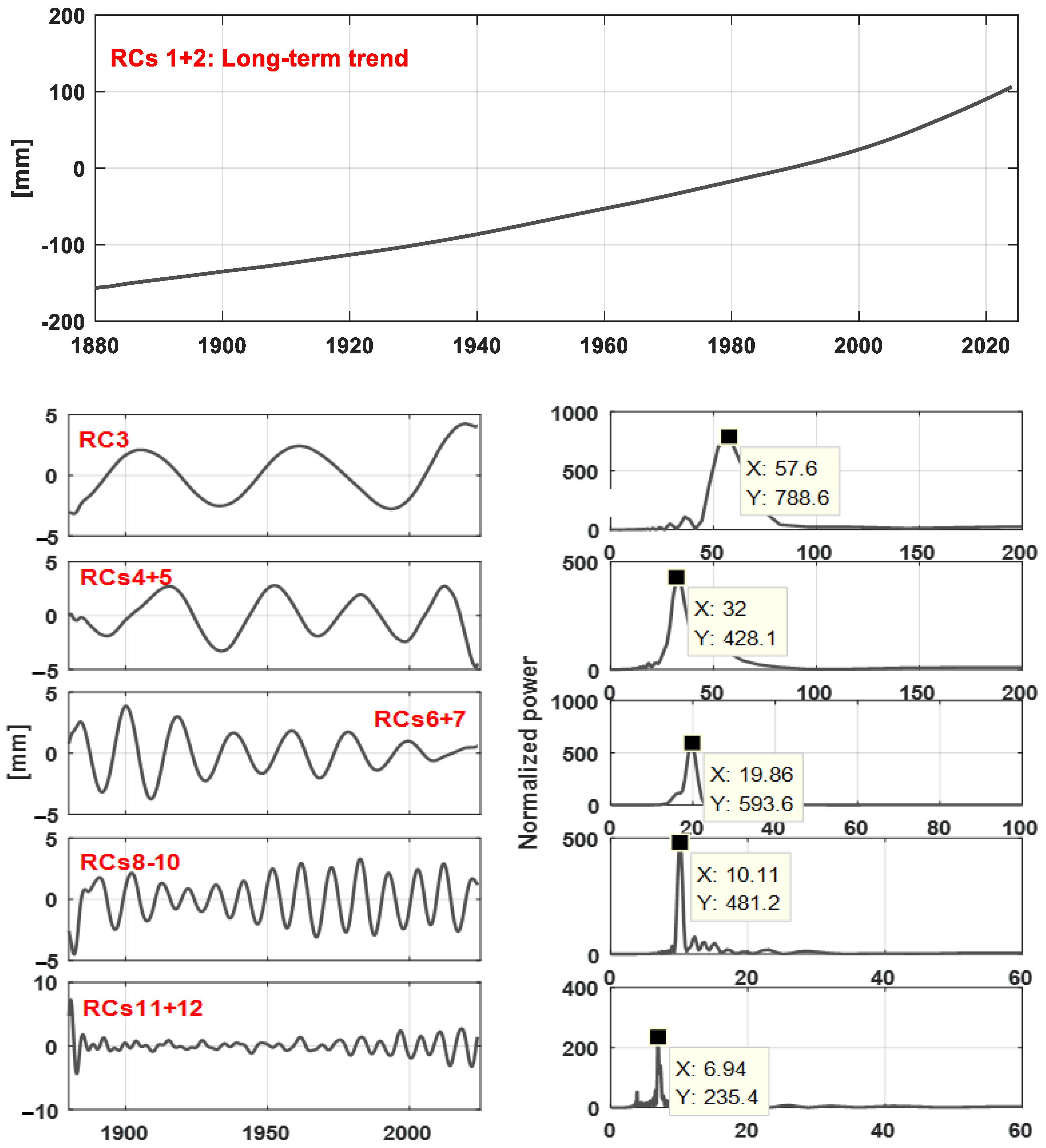
3.2. Analysis of Global Mean Sea Level Changes from 1880 to 2023

The GMSL time series and its uncertainty are presented in Figure 5. For the real GMSL change series, a window size of 720 is selected, and upon analyzing the periodic harmonic components, 12 is determined as the reconstructed order for extracting GMSL change signals. Figure 6 illustrates the six groups of components reconstructed by the traditional SSA and their respective periodograms. It is reasonable to conclude that the first two reconstructed components (RCs 1-2) are primarily associated with the long-term trend. The periodograms of the other five groups—RCs 3, RCs 4-5, RCs 6-7, RCs 8-10 and RCs 11-12—are also shown in Figure 6. These periodograms reveal the influences of the Pacific Decadal Oscillation (PDO), the El Niño-Southern Oscillation (ENSO) and sunspots on the GMSL time series. The periods of the PDO, ENSO and sunspots are approximately 20–30 years (RCs 4-5), 20–25 years (RCs 6-7) and 10–11 years (RCs 8-10), respectively [30,31]. Additionally, a significant 57-year oscillation (RC 3) is observed in the GMSL change series, which aligns well with the findings of Church and White [17] and Chambers et al. [32]. Therefore, RCs 1-12 are identified as GMSL signals, while RCs 11-720 are considered noise.

The fitting error (${\sigma }_{\mathrm{W}}$) of the weighted SSA is estimated by [23]

$${\sigma }_{\mathrm{W}}=\sqrt{{\displaystyle \frac{1}{N}}{\displaystyle \sum _{i=1}^N{p}_i{(x_i-{\widehat{x}}_i^{\mathrm{W}})}^2}}$$

(17)

Similarly, the fitting error (${\sigma }_{\mathrm{T}}$) of the traditional SSA is estimated by

$${\sigma }_{\mathrm{T}}=\sqrt{{\displaystyle \frac{1}{N}}{\displaystyle \sum _{i=1}^N{(x_i-{\widehat{x}}_i^{\mathrm{T}})}^2}}$$

(18)

where, ${\widehat{x}}_i^{\mathrm{T}}$ and ${\widehat{x}}_i^{\mathrm{W}}$ are the signals reconstructed with the traditional SSA and weighted SSA at the ith epoch. The fitting errors induced for the GMSL time series using 12 PCs are 4.99 mm and 5.58 mm for the weighted SSA and traditional SSA, respectively, with a relative improvement of approximately 10.57% achieved by the weighted SSA over the traditional SSA, indicating that the weighted SSA outperforms the traditional SSA in terms of extracting signals.

3.3. Prediction of Global Mean Sea Level Changes from 2024 to 2100

Based on the above analysis results, we forecast future GMSL change series from 2024 to 2100 via the linear recurrent forecasting method using the weighted SSA and traditional SSA. Considering the impact of adopting different RCs on the GMSL change prediction results, we separately use RCs 1-2 (long-term trend) and RCs 1-12 (long-term trend and periodic components) to forecast the future GMSL changes. Note that the corresponding uncertainty is estimated by the Monte Carlo algorithm under 95% confidence intervals. Figure 7 shows the future GMSL changes from 2024 to 2100 predicted by the weighted SSA and traditional SSA with RCs1-2 (long-term trend) and RCs 1-12 (long-term trend and periodic components).

Figure 7 shows that a relatively small sea level rise can be obtained when predicting using only the first two reconstructed components (i.e., the long-term trend) rather than including additional periodic components. The predicted Global Mean Sea Level (GMSL) changes using weighted SSA from 2024 to 2100, based on RCs 1-12, are 215.17 ± 17.38 mm for 2050 and 868.90 ± 147.42 mm for 2100, with respect to the same baseline from 1995 to 2014 as that of the IPCC AR6 report. These values are larger than those produced by the traditional SSA, which are 210.97 ± 13.54 mm for 2050 and 814.62 ± 112.84 mm for 2100. Regarding the first two reconstructed components (RCs 1-2), the future GMSL changes for the year 2050 are 208.50 ± 6.62 mm using the weighted SSA and 197.83 ± 6.74 mm using the traditional SSA. For the year 2100, the changes are 796.75 ± 55.92 mm using the weighted SSA and 705.25 ± 53.73 mm using the traditional SSA. Note that forecasting future GMSL change by considering periodic components introduces relatively larger uncertainty. The corresponding prediction results of GMSL change from 2030 to 2100, with a step size of 10 years, are presented in

Table 3. The prediction of future GMSL change by weighted SSA and traditional SSA (unit: mm).

Index	Year	Traditional SSA		Weighted SSA		IPCC AR6
		RCs1-2	RCs1-12	RCs1-2	RCs1-12	Medium Confidence SSP5-8.5
Validation	2020	54.01 ± 0.81	54.51 ± 1.02	55.13 ± 0.79	54.15 ± 1.32	51.0 ± 6.99
Prediction	2030	91.86 ± 2.01	94.46 ± 3.88	94.60 ± 1.94	95.90 ± 5.50	102.0 ± 14.59
	2040	140.01 ± 3.86	152.30 ± 8.60	145.81 ± 3.76	158.07 ± 12.35	163.0 ± 24.52
	2050	197.83 ± 6.74	210.97 ± 13.54	208.50 ± 6.62	215.17 ± 17.38	243.0 ± 36.96
	2060	266.20 ± 11.01	287.05 ± 21.90	284.03 ± 10.93	298.09 ± 29.64	325.0 ± 52.11
	2070	347.43 ± 17.16	385.11 ± 35.73	375.54 ± 17.22	404.27 ± 47.11	427.0 ± 71.93
	2080	445.53 ± 25.78	495.70 ± 54.72	488.39 ± 26.17	516.21 ± 69.65	541.0 ± 96.02
	2090	563.64 ± 37.62	638.62 ± 79.34	627.02 ± 38.66	677.40 ± 103.49	674.0 ± 122.22
	2100	705.25 ± 53.73	814.62 ± 112.84	796.75 ± 55.92	868.90 ± 147.42	830.0 ± 152.42

. Note that the IPCC AR6 sea-level rise projections are adopted as the comparisons. For the year 2020, the GMSL rise is ~54 mm, close to 51.0 ± 4.11 mm of IPCC AR6 with the medium confidence under the high-emission scenarios (SSP5-8.5). Therefore, we presented the IPCC AR6 Medium confidence SSP5-8.5 datasets in Table 3. It is obvious to find that using the first 12 RCs to forecast future GMSL rise can have closer predicted estimates with respect to those results from the IPCC AR6 report, indicating that considering all related GMSL reconstructed components and formal errors of data series can better forecast the future GMSL rise. One thing that needs to be mentioned is that the uncertainty of IPCC AR6 in Table 3 is estimated using the sea level projections at different quantiles (0.10–0.90) of the probability box of the sea level change variable.

4. Discussion

Considering that the IPCC assessment reports normally mainly forecast the future sea level rise in view of a long-term trend by integrating various lines of evidence from climate models, historical observations and theoretical understandings of physical processes, maybe they can be compared to the predicted GMSL changes by SSA predictions to validate their reliability to some extent. The IPCC AR6 report noted that under high-emission scenarios (SSP5-8.5), the global mean sea level (GMSL) is projected to increase by 243.0 ± 36.96 mm by 2050 and by 830.0 ± 152.42 mm by 2100 [8,33], consistent with 855 mm from the special report on the Ocean and Cryosphere in a Changing Climate [34], which covers the predicted GMSL change. When long-term trend RCs 1-12 are selected for predicting the GMSL change, the predicted GMSL change by the weighted SSA by 2100 is 868.90 ± 147.42 mm, which is closer to the median predicted value of 855 mm from the special report on the Ocean and Cryosphere in a Changing Climate [34] and more consistent with 830.0 ± 152.42 m in the IPCC AR6 report than those yielded by the traditional SSA, indicating that the weighted SSA can forecast future GMSL changes more reliably than the traditional SSA to some extent. However, there still existed some differences between the predicted GMSL changes of some previous publications and those in this study. For example, Elneel et al. [21] developed stochastic auto-regressive ARIMA-type models to forecast sea levels, whose results show an increase up to 350 mm by the year 2100, mainly due to the different methods and datasets adopted.

Based on the predicted GMSL change, we further estimate the GMSL change rates and accelerations of three timespans, namely, 1880–2023 (history data-observed), 2024–2100 (future-forecasted) and 1880–2100 (whole period), which are presented in

Table 4. The GMSL change rates and accelerations of different timespans for the weighted SSA.

Year	Rate [mm/year]		Acceleration [mm/year2]
	RCs1-2	RCs1-12	RCs1-2	RCs1-12
1880–2023	1.70 ± 0.02	1.70 ± 0.02	0.015 ± 0.001	0.016 ± 0.001
2024–2100	9.14 ± 1.28	9.92 ± 1.79	0.180 ± 0.040	0.206 ± 0.120
1880–2100	3.72 ± 0.26	3.54 ± 0.74	0.052 ± 0.008	0.056 ± 0.020

. Here, we use only the GMSL changes predicted by the weighted SSA. For the period from 1880 to 2023, the GMSL change rate is 1.71 ± 0.02 mm/year, which is close to that estimated using the reconstructed GMSL signals from RCs 1-2 and RCs 1-12 via the weighted SSA, with an acceleration of 0.015 ± 0.001 mm/year². However, from 2024 to 2100, the GMSL will increase at a relatively large rate, ranging from 9.14 mm/year to 9.92 mm/year, with a 0.18–0.21 mm/year² increase, which is consistent with the conclusion that the GMSL change rate is expected to accelerate further to rates of 5.2–12.1 mm/year [35,36]. For the whole period from 1880 to 2100, the GMSL change rates and accelerations are 3.72 ± 0.26 mm/year and 3.54 ± 0.74 mm/year and 0.052 ± 0.008 mm/year² and 0.056 ± 0.02 mm/year², respectively, based on RCs1-2 and RCs1-12.

Compared with GMSL rise, regional sea level change has significant differences and impacts on coastal regions—for example, Vecchio et al. [10] forecasted a sea level rise up to 2150 in the northern Mediterranean coasts and found that the effects of tectonics and other local factors should be properly considered, which results in significant differences with respect to the IPCC report. Therefore, more detailed analysis needs be conducted to evaluate the reliability of the sea level projections by the weighted SSA in the future.

5. Conclusions

This paper adopts historical global mean sea level data to predict global mean sea level rises. To more efficiently forecast future sea level changes, a weighted SSA approach is proposed by considering the formal errors induced by the GMSL time series. The statistical results of simulation experiments show that all the RMSEs and MAEs induced by the weighted SSA are smaller than those of the traditional SSA, indicating that the weighted SSA can forecast GMSL sea level changes more accurately than the traditional SSA, regardless of the utilized prediction length. For the real past GMSL change from 1880 to 2023, the rate of change was 1.70 ± 0.02 mm/year, and the acceleration was 0.015 ± 0.001 mm/year². When predicting future GMSL changes based on RCs 1-2 and RCs 1-12, the global mean sea level will increase by 796.75 ± 55.92 mm and 868.90 ± 147.42 mm for weighted SSA and 705.25 ± 53.73 mm and 814.62 ± 112.84 mm for traditional SSA at the year 2100, with respect to the same baseline from 1995 to 2014 as that of the IPCC AR6 report, respectively. The GMSL change predicted by the weighted SSA by 2100 is close to the median predicted value of 855 mm from the special report on the Ocean and Cryosphere in a Changing Climate [34] and more consistent with 830.0 ± 152.42 m in the IPCC AR6 report under high-emission scenarios (SSP5-8.5) than those yielded by the traditional SSA, indicating that the weighted SSA can forecast future GMSL changes more reliably than the traditional SSA to some extent. Overall, it is reasonable to conclude that the weighted SSA can forecast GMSL changes accurately and reliably by considering formal errors, which highlights the necessity of considering formal errors when forecasting future GMSL changes based on past GMSL data.

References

1. Ellison, A.M.; Farnsworth, E.J. Anthropogenic disturbance of Caribbean Mangrove Ecosystems: Past impacts, present trends, and future predictions. Biotropica 1996, 28, 549–565. [Google Scholar] [CrossRef]
2. Cronk, J.K.; Fennessy, M.S. Wetland Plants: Biology and Ecology; CRC Press LLC: Boca Raton, FL, USA, 2001. [Google Scholar]
3. Anthoff, D.; Nicholls, R.J.; Tol, R.S.; Vafeidis, A.T. Global and Regional Exposure to Large Rises in Sea-Level: A Sensitivity Analysis. Tyndall Centre for Climate Change Research-Working Paper 96. 2006. Available online: http://www.tyndall.ac.uk/sites/default/files/wp96_0.pdf (accessed on 20 May 2024).
4. Hoegh-Guldberg, O.; Bruno, J.F. The impact of climate change on the world’s marine ecosystems. Science 2010, 328, 1523–1528. [Google Scholar] [CrossRef]
5. Nicholls, R.J.; Cazenave, A. Sea-level rise and its impact on coastal zones. Science 2010, 328, 1517–1520. [Google Scholar] [CrossRef] [PubMed]
6. Cazenave, A.; Hamlington, B.; Horwath, M.; Barletta, V.R.; Benveniste, J.; Chambers, D.; Döll, P.; Hogg, A.E.; Legeais, J.F.; Merrifield, M.; et al. Observational Requirements for Long-Term Monitoring of the Global Mean Sea Level and Its Components over the Altimetry Era. Front. Mar. Sci. 2019, 6, 582. [Google Scholar] [CrossRef]
7. Meehl, G.A.; Stocker, T.F.; Collins, W.D.; Friedlingstein, P.; Gaye, A.T.; Gregory, J.M.; Kitoh, A.; Knutti, R.; Murphy, J.M.; Noda, A.; et al. Global climate projections. In Climate Change 2007: The Physical Science Basis. Contribution of Working Group I to the Fourth Assessment Report of the Intergovernmental Panel on Climate Change; Solomon, S., Qin, D., Manning, M., Chen, Z., Marquis, M., Averyt, K.B., Tignor, M., Miller, H.L., Eds.; Cambridge University Press: Cambridge, UK, 2007. [Google Scholar]
8. IPCC AR6. Monitoring and Projections of Global and Regional Sea Level Change. 2022. Available online: https://www.ipcc.ch/report/sixth-assessment-report-cycle/ (accessed on 20 May 2024).
9. Moorhead, K.K.; Brinson, M.M. Response of Wetlands to Rising Sea Level in the Lower Coastal Plain of North Carolina. Ecol. Appl. 1995, 5, 261–271. [Google Scholar] [CrossRef]
10. Vecchio, A.; Anzidei, M.; Serpelloni, E. Sea level rise projections up to 2150 in the northern Mediterranean coasts. Environ. Res. Lett. 2023, 19, 014050. [Google Scholar] [CrossRef]
11. Vaziri, M. Predicting Caspian Sea surface water level by ANN and ARIMA models. J. Waterw. Port Coast. Ocean Eng. 1997, 123, 158–162. [Google Scholar] [CrossRef]
12. IPCC AR5. Climate Change 2013, IPCC Fifth Assessment Report. 2013. Available online: http://www.ipcc.ch/report/ar5/ (accessed on 25 March 2024).
13. Pfeffer, W.T.; Harper, J.T.; O’Neel, S. Kinematic constraints on glacier contributions to 21st century sea-level rise. Science 2008, 321, 1340–1343. [Google Scholar] [CrossRef]
14. Rahmstorf, S. A semi-empirical approach to projecting future sea-level rise. Science 2007, 315, 368–370. [Google Scholar] [CrossRef]
15. Domingues, C.M.; Church, J.A.; White, N.J.; Gleckler, P.J.; Wijffels, S.E.; Barker, P.M.; Dunn, J.R. Improved estimates of upper-ocean warming and multi-decadal sea-level rise. Nature 2008, 453, 1090–10931093. [Google Scholar] [CrossRef]
16. Grinsted, A.; Moore, J.C.; Jevrejeva, S. Reconstructing sea level from paleo and projected temperatures 200 to 2100 AD. Clim. Dyn. 2009, 34, 461–472. [Google Scholar] [CrossRef]
17. Church, J.; White, N. Sea-level rise from the late 19th to the early 21st century. Surv. Geophys. 2011, 32, 585–602. [Google Scholar] [CrossRef]
18. GSFC. Global Mean Sea Level Trend from Integrated Multi-Mission Ocean Altimeters TOPEX/Poseidon, Jason-1, OSTM/Jason-2, and Jason-3 Version 5.1. Ver. 5.1 PO.DAAC, CA, USA, 2021. Available online: https://doi.org/10.5067/GMSLM-TJ151 (accessed on 20 May 2024).
19. Golyandina, N.; Zhigljavsky, A. Singular Spectrum Analysis for Time Series; Springer: Berlin/Heidelberg, Germany, 2013; p. 119. [Google Scholar] [CrossRef]
20. Vermeer, M.; Rahmstorf, S. Global sea level linked to global temperature. Proc. Natl. Acad. Sci. USA 2009, 106, 21527–21532. [Google Scholar] [CrossRef]
21. Elneel, L.; Zitouni, M.S.; Mukhtar, H.; Al-Ahmad, H. Examining sea levels forecasting using autoregressive and prophet models. Sci. Rep. 2024, 14, 14337. [Google Scholar] [CrossRef]
22. Vautard, R.; Ghil, M. Singular spectrum analysis in nonlinear dynamics with applications to paleoclimatic time series. Phys. D Nonlinear Phenom. 1989, 35, 395–424. [Google Scholar] [CrossRef]
23. Wang, F.; Shen, Y.; Li, W.; Chen, Q. Singular spectrum analysis for heterogeneous time series by taking its formal errors into account. Acta Geodyn. Geomater. 2018, 15, 395–403. [Google Scholar] [CrossRef]
24. Li, W.; Shen, Y. The Consideration of Formal Errors in Spatiotemporal Filtering Using Principal Component Analysis for Regional GNSS Position Time Series. Remote Sens. 2018, 10, 534. [Google Scholar] [CrossRef]
25. Shen, Y.; Wang, F.; Chen, Q. Weighted multichannel singular spectrum analysis for post-processing GRACE monthly gravity field models by considering the formal errors. Geophys. J. Int. 2021, 226, 1997–2010. [Google Scholar] [CrossRef]
26. Vautard, R.; Yiou, P.; Ghil, M. Singular-spectrum analysis: A toolkit for short, noisy, chaotic signals. Phys. D Nonlinear Phenom. 1992, 58, 95–126. [Google Scholar] [CrossRef]
27. Livezey, R.E.; Chen, W.Y. Statistical Field Significance and its Determination by Monte Carlo Techniques. Mon. Weather. Rev. 1983, 111, 46–59. [Google Scholar] [CrossRef]
28. Davis, J.L.; Mitrovica, J.X. Glacial isostatic adjustment and the anomalous tide gauges record of eastern North America. Nature 1996, 379, 331–332. [Google Scholar] [CrossRef]
29. Garner, G.G.; Hermans, T.; Kopp, R.E.; Slangen, A.B.A.; Edwards, T.L.; Levermann, A.; Nowikci, S.; Palmer, M.D.; Smith, C.; Fox-Kemper, B.; et al. IPCC AR6 Sea-Level Rise Projections. Version 20210809. PO.DAAC, CA, USA, 2021. Available online: https://podaac.jpl.nasa.gov/announcements/2021-08-09-Sea-level-projections-from-the-IPCC-6th-Assessment-Report (accessed on 18 June 2024).
30. Chen, J.; Wilson, C.; Chambers, D.; Nerem, R.; Tapley, B. Seasonal global water mass budget and mean sea level variations. Geophys. Res. Lett. 1998, 25, 3555–3558. [Google Scholar] [CrossRef]
31. Nerem, R. Measuring global mean sea level variations using TOPEX/POSEIDON altimeter data. J. Geophys. Res. Ocean. 1995, 100, 25135–25151. [Google Scholar] [CrossRef]
32. Chambers, D.; Merrifield, M.; Nerem, R. Is there a 60-year oscillation in global mean sea level? Geophys. Res. Lett. 2012, 39, L18607. [Google Scholar] [CrossRef]
33. Zhang, T.; Yu, Y.; Xiao, C.; Hua, L.; Yan, Z. Interpretation of IPCC AR6 report: Monitoring and projections of global and regional sea level change. Adv. Clim. Chang. Res. 2022, 18, 12–18. [Google Scholar] [CrossRef]
34. Oppenheimer, M.; Glavovic, B.; Hinkel, J.; van de Wal, R.; Magnan, A.K.; Abd-Elgawad, A.; Sebesvari, Z. Sea Level Rise and Implications for Low-Lying Islands, Coasts and Communities. In IPCC Special Report on the Ocean and Cryosphere in a Changing Climate; Pörtner, H.-O., Roberts, D.C., Masson-Delmotte, V., Zhai, P., Tignor, M., Poloczanska, E., Mintenbeck, K., Alegría, A., Nicolai, M., Okem, A., et al., Eds.; Cambridge University Press: Cambridge, UK; New York, NY, USA, 2019; pp. 321–445. [Google Scholar] [CrossRef]
35. Oelsmann, J.; Marcos, M.; Passaro, M.; Sanchez, L.; Dettmering, D.; Dangendorf, S.; Seitz, F. Regional variations in relative sea-level changes influenced by nonlinear vertical land motion. Nat. Geosci. 2024, 17, 137–144. [Google Scholar] [CrossRef]
36. Fox-Kemper, B.; Hewitt, H.T.; Xiao, C.; Aðalgeirsdóttir, G.; Drijfhout, S.S.; Edwards, T.L.; Golledge, N.R.; Hemer, M.; Kopp, R.E.; Krinner, G.; et al. Climate Change 2021: The Physical Science Basis; Masson-Delmotte, V., Zhai, P., Pirani, A., Connors, S.L., Péan, C., Berger, S., Caud, N., Chen, Y., Goldfarb, L., Gomis, M.I., et al., Eds.; Cambridge University Press: Cambridge, UK, 2021; Chapter 9. [Google Scholar]
Figure 1. The simulated noisy GMSL change series and true signals.
Jmse 12 02124 g001
Figure 2. The predicted sea level rise for simulation experiments by weighted SSA and traditional SSA with the predicted length from 10 years to 60 years with a step size of 10 years.
Jmse 12 02124 g002
Figure 3. The RMSEs of 100 simulations by weighted SSA and traditional SSA for predicting different lengths from 10 years to 60 years with a step size of 10 years.
Jmse 12 02124 g003
Figure 4. The MAEs of 100 simulations by weighted SSA and traditional SSA for predicting different lengths from 10 years to 60 years with a step size of 10 years.
Jmse 12 02124 g004
Figure 5. The merged global mean sea level change series using tide gauge and altimetry datasets and its uncertainty from January 1880 to December 2023. Note. The merged series are set to have the same baseline over 1995–2014 as that of the IPCC AR6 report.
Jmse 12 02124 g005
Figure 6. The reconstructed GMSL components of six groups by traditional SSA and their periodograms. Note. RCs1-2 are mainly related to the long-term trend; the other five groups are specifically 3, 4-5, 6-7, 8-10 and 11-12.
Jmse 12 02124 g006
Figure 7. The predicted GMSL changes by weighted SSA and traditional SSA using the first two RCs (long-term trend) and twelve RCs (long-term trend and periodic components) for the period from 2024 to 2100. Note. The vertical dashed line at December 2023 to clearly show the boundary between the observation data (1880–2023) and predicted data (2024–2100).
Jmse 12 02124 g007