Numerical Study on the Hydrodynamics of Manta Rays Exiting Water

Abstract

Observation of manta rays exiting water has been rarely reported, as there are various difficulties in observing and obtaining data on their behavior in a marine environment. Therefore, the movement mechanism of manta rays exiting water is still unclear. This paper proposes the idea of using CFD (based on Ansys Fluent, version 2022) to simulate the water-exit process of the manta ray. The study discusses the changes in the mechanical and kinematic parameters of the manta ray over time and obtains the evolution of vortex structures during the underwater movement phase of the manta ray. Time history variations of the mechanical and kinematics parameters in the vertical water-exit motion are discussed. The evolution of vortex structures during the underwater movement of the manta ray is obtained. The direction in which the manta ray approaches the free surface is the X-direction and the direction of its flapping motion is the Z-direction. V_X and V_Z are the velocities of the manta ray in the X- and Z-directions, respectively. F_X and F_Z represent the forces acting on the manta ray in the X- and Z-directions, respectively. The results indicate that the vertical water-exit of the manta ray mainly undergoes three stages: underwater acceleration, crossing the free surface, and aerial movement. During the underwater acceleration phase, the force F_X of the manta ray fluctuates, but its average value is positive within one cycle. V_X also shows a stepwise increase, while F_Z and V_Z exhibit periodic changes. During the stage of crossing the free liquid surface, F_X first increases and then sharply decreases, V_X also shows an increase and then decrease, F_Z fluctuates greatly, producing a peak, and the swimming speed V_Z of the manta ray is negative. During the aerial motion phase, F_X is mainly affected by gravity, V_X decreases linearly, F_Z approaches 0, and V_Z remains constant. During the process of swimming underwater, the tail vortex of the manta ray presents a double row staggered structure to generate thrust. Increasing the flapping frequency and decreasing the wave number can improve the swimming speed of the manta ray, and then increase its water-exit height. The findings may provide an important hydrodynamics basis for biomimetic trans-media vehicle designs.

1. Introduction

There are some special creatures in the ocean which with their unique body structure can leap from water into air, and even glide in the air, among which representatives are flying fish, whales and dolphins. They use their powerful tails to beat the water and lift their bodies into the air. Similarly to whales and dolphins, manta rays also have a habit of coming out of the water, potentially reaching a height of 2 m, so they are also called flying manta rays. The manta ray has a large, flat, diamond-shaped body [1] with a pair of pectoral fins with a high aspect ratio and a wingspan of up to 9 m [2,3]. Manta rays swim underwater and exit water powered mainly by pectoral fin flapping, similar to flying birds. The water-exit process involves an interaction between solid and fluid under the influence of a free surface, which is a classic problem in the field of fluid mechanics and has important engineering application value in the field of ship and ocean engineering and underwater weapons.

In in vivo experiments, the dynamic and kinematic characteristics of fish swimming can be observed, and the flow field information can be measured. The main means are high-speed camera technology and velocity digital imaging technology. Heine [4] recorded the complete kinematic data of the bull-noted ray through experimental observation of its swimming state, obtaining the relationship between swimming speed, pectoral fin flapping amplitude, and frequency and wavelength transmitted by the pectoral fins, and suggested that the bull-noted ray moved in a lift mode. Rosenberger [1] observed the swimming mode, perch position and lifestyle of eight different types of rays and calculated the shape parameters and movement parameters. Among them, the beating frequency of the bull-nosed ray was the lowest and the amplitude was the largest. Blevins et al. [5] recorded the movements of 31 points on the pectoral fins of stingrays during slow and fast swimming by using high-speed camera technology and analyzed the fluctuation parameters on the pectoral fin surface of rays under three-dimensional conditions. They found that the movement frequency and wave speed were the main reasons for the improvement in the swimming speed of stingrays. Russo et al. [6] used computed tomography to compare the effects of bone arrangement, connectional tissue and shape on the pectoral fin movement of Dasyatis sabina and the cownose ray. A biomechanical model was established to predict the three-dimensional deformation of pectoral fins and axial strain between bones. Among them, the cownose ray showed flexible deformation in both the spanwise and chordwise directions of pectoral fins. Fish et al. [7] used high-speed cameras to observe the motion morphology of manta rays and established a kinematic model of the pectoral fin flutter of the bulb-nosing ray, calculated the relationship between swimming speed, frequency and amplitude, and found the wave characteristics of manta rays in the direction of spread and the direction of chord. Subsequently, Fish [8] assessed the free-swimming tail-vortices of the cownose ray measured by DPIV, and found that When the pectoral fins flap upwards or downwards, one vortex falls off each, forming a 2S vortex. Zhang et al. [9] recorded the motion trajectory of the cownose ray during active propulsion, turning and gliding, and established the pectoral fin deformation equation, obtaining a series of statistical parameters, such as the up-and-down amplitude and the ratio of the up-and-down amplitude, glide attitude angle and height of the pectoral fin during gliding using statistical analysis. However, it is very difficult to carry out controlled experiments in live animals to study the various swimming behaviors of manta rays. Benefiting from the development of CFD technology, most of the issues in the biomimetic area that are impossible to solve using traditional methods can now be investigated through numerical simulation. Liu et al. [10] calculated the force and tail vortex structure of manta rays using an immersed boundary solver method, finding that most of the thrust was generated by the distal part of the pectoral fin and that the powerful jet induced by the vortex ring in the wake was the main reason for thrust generation. Thekkethil et al. [11] used an immersion boundary solver method to study the evolution of tail vortex in the motion of the ray and cownose ray, and the study showed that the tail vortex of the ray pattern is a double row vortex composed of vortex rings, while the cownose ray pattern is a horseshoe vortex composed of multiple vortex rings. Zhang et al. [9,12] combined a submerged boundary solver method and a gas kinetics scheme based on spherical function, proposing an improved IB-SGKS method to solve the mesh distortion caused by large deformation, and studied the effects of pectoral fin stringed deformation and amplitude asymmetry on the hydrodynamic performance and eddy dynamics of manta rays. The results showed that appropriate chord deformation can increase thrust and improve efficiency. The tip vortex is the main source of thrust, while the leading-edge vortex and the trailing-edge vortex are not conducive to thrust generation. Menzer et al. [13] studied the hydrodynamic performance of manta rays and the change in the leading-edge vortex and found that the pitch angle of the pectoral fins had a significant impact on thrust and efficiency. When the pitch angle was small, the thrust was large, and there was setting of the pitch angle and bending of the angle of the pectoral fins to maximize the propulsion efficiency. Fish et al. [8] calculated the forward swimming speed and autonomous swimming efficiency of manta rays at different movement frequencies. The experimental results showed that the forward swimming velocity increased with increase in frequency, and that the steady-state velocity was 1.5 times the body length after non-dimensionalization. The maximum efficiency of autonomous swimming could reach 89%. Based on the OpenFoam computing platform, Bianchi et al. [14] established a numerical calculation model of single degree of freedom autonomous swimming of the cownose ray by using overlapping grid technology. The effects of pectoral fin flutter frequency and wavelength on thrust, power and swimming speed were studied, and the tail vortex structure was analyzed. The results showed that the steady-state swimming speed of the bull-nosed ray was proportional to the frequency. In addition, there have been many studies on the hydrodynamic characteristics of rigid bodies coming out of water and these studies have produced many important discoveries on the mechanism of bodies coming out of water. Xing et al. [15] proposed a novel bionic pectoral fin and experimentally studied the effects of the oscillation parameters on the hydrodynamic performance of a bionic experimental prototype. Manduca et al. [16] proposed a novel control strategy for an underactuated robotic fish. The control strategy was inspired by central pattern generators (CPGs) to control the torque exerted on the fishtail. Mo et al. [17] proposed an FTALOS guidance subsystem to achieve a planar path following a bio-inspired robotic fish equipped with a compliant and flexible tail fin driven by a cable mechanism. Miao [18] conducted an experiment to study the problem of the forced uniform exhalation of a two-dimensional cylinder, obtaining the exhalation process of an object using high-speed photography technology, and measured the pressure change on the surface of the object with a pressure sensor. Liju et al. [19] conducted experimental research on the forced water movement of axisymmetric bodies and studied the deformation of a free liquid surface under different scales, Froude number and fluid medium conditions. Moreover, the boundary element method (BEM) based on potential flow theory was used to simulate the deformation of a free liquid surface of the axisymmetric rigid body. Colicchio et al. [20] studied the water discharge of a horizontal cylinder and performed detailed measurements of the velocity field and local load around the cylinder. Based on the finite volume method, Moshari et al. [21] simulated the water discharge of a horizontal cylinder under buoyancy by using the VOF method and dynamic grid technology and studied the influence of the deformation of a free surface and the mass of the cylinder. Ye et al. [22] studied the nonlinear problem of the large angle oblique water discharge of an axisymmetric body using a perturbation method. Zhang et al. [23] used PIV technology to study the transient flow field near the free surface when an object exits water at a constant velocity, and quantitatively obtained the transient history of the near free surface when an object exits water. Xia et al. [24] simulated the hydrodynamic characteristics of dolphin jumping behavior and discussed the changes in the kinematic parameters and capability parameters with time. Hou et al. [25] used dynamic grid technology and a VOF multiphase flow model to numerically simulate the effluent process of squid. It was found that, during the process of pushing from water to air, the cuttlefish chose a propulsive priority strategy rather than a propulsive efficiency priority strategy. The maximum flight speed was negatively correlated with the underwater launch angle. However, no reports have been published on the hydrodynamic characteristics of manta rays exiting water.

Based on the VOF multiphase flow model, a coupled dynamic equation and fluid mechanics equation, a numerical model of the manta ray’s vertical water exit was established by using an overlapping grid technique. The dynamics of manta rays exiting water was studied quantitatively, and the transient evolution of the fluid structure was analyzed. These results can provide an important hydrodynamics basis for the design of bionic trans-media underwater vehicles.

2. Physical Model and Kinematics Model

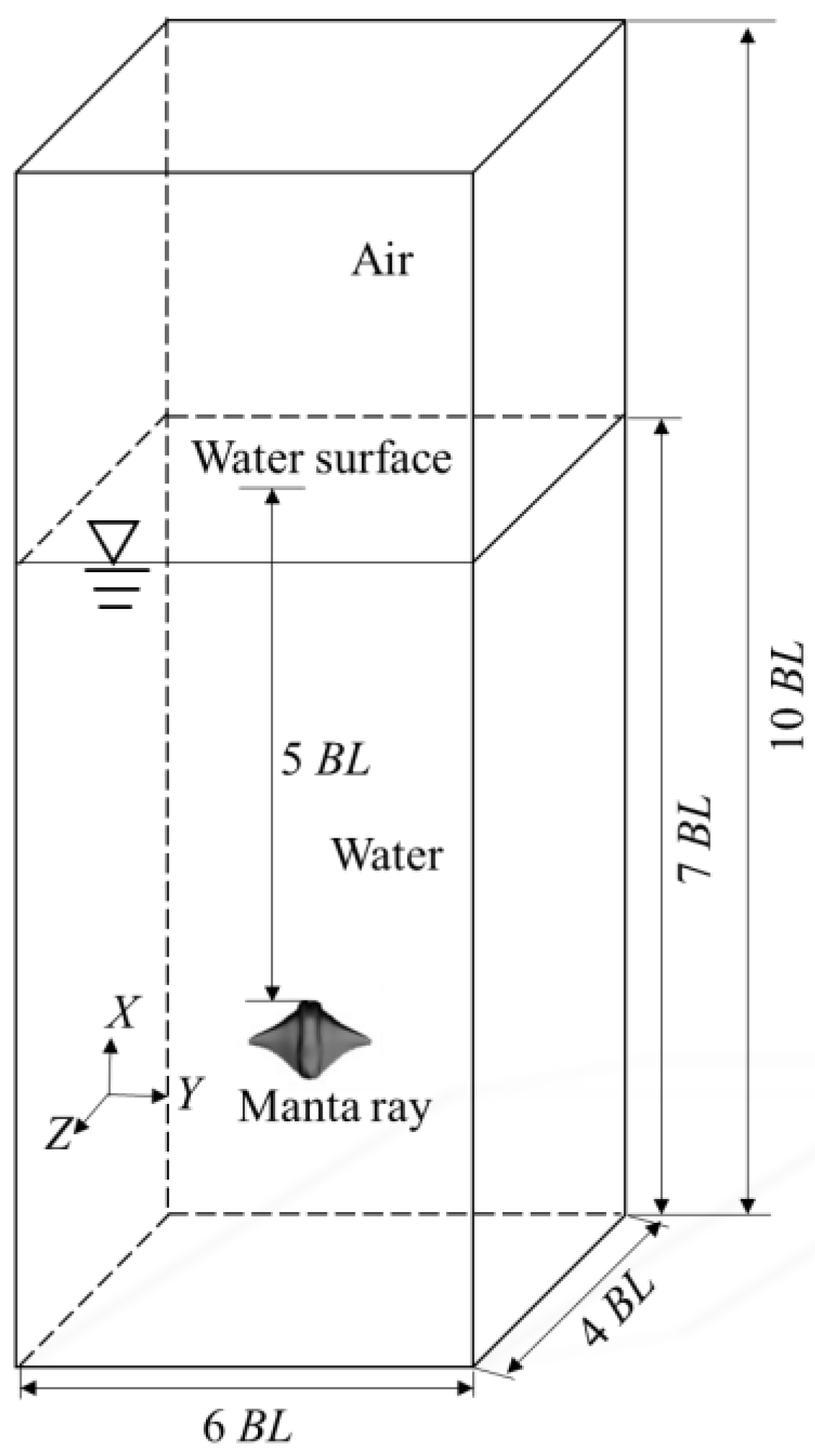
2.1. Physical Model

The shape of the manta ray was built using reverse engineering technology, that is, the coordinate point positions on the surface of the manta ray were obtained through three-dimensional scanning; three-dimensional curves and further three-dimensional surfaces were constructed through the point data, and finally, the three-dimensional model of the physical object was reconstructed. The snout fins, eyes, dorsal fin and tail whip of the manta ray were simplified and were not reflected in the model. The final physical model is shown in Figure 1a. It can be seen that the physical model of the manta ray has a high agreement with the real biological shape. The body layout of the manta ray is wing-body fusion, the body length BL is 1800 mm, the stretch length SL is 1450 mm, the maximum thickness A is 35 mm, the width of the fish body B is 300 mm, and the mass m is 432 kg. In Figure 1, o-xyz is the body-fixed coordinate system of the manta ray. The apex of the manta ray’s head is taken as the origin, the line between the head and tail is the x-axis, the spanwise direction of the right pectoral fin is the y-axis, and the direction of the pectoral fin is the z-axis.

2.2. Kinematics Model

In a body-fixed coordinate system o-xyz, any point on the pectoral fin at the initial time is (x_f, y_f, z_f), and the pectoral fin deformation at any time t is (x(x_f, y_f, t), y(x_f, y_f, t), z(x_f, y_f, t)). Considering the span-chord deformation of the pectoral fin, its equation of motion can be described as follows [9]:

$$\left\{\begin{array}{c}x\left(x_f,y_f,t\right)=x_f\hfill \\ y\left(x_f{y}_f,t\right)=a\left(t\right)y_f\left(1-\left(1-k\right)\left|\theta \left(t,x_f\right)\right|y_f/SL\right)cos\left[{\theta }_{max}{y}_f/SL\cdot \theta \left(t,x_f\right)\right]\hfill \\ z\left(x_f{y}_f,t\right)=z_f+a\left(t\right)y_f\left(1-\left(1-k\right)\left|\theta \left(t,x_f\right)\right|y_f/SL\right)sin\left[{\theta }_{max}{y}_f/SL\cdot \theta \left(t,x_f\right)\right]\hfill \\ \theta \left(x_f,t\right)=sin\left(\omega t-2\mathrm{\pi }W{x}_f/BL\right)\hfill \end{array}\right.$$

(1)

where ω, = 2πf, f is the pectoral fin flapping frequency; $W$ is the wave number, which represents the number of complete traveling waves in the chordal direction of the pectoral fin, $W$ is defined as $W=BL/\lambda$, and $\lambda$ is the wavelength of the chordal traveling wave. As shown in Figure 1b, it is assumed that the spanwise curve can be treated as an arc $\stackrel{⌢}{OT}$ with a radius of $l$. The deviation angle θ is defined by the straight line OT joining the fin root and tip. When the fin tip reaches the highest position, the parameter k represents the ratio of the straight line OT to the arc length $\stackrel{⌢}{OT}$, i.e., $k=2l\sin {\theta }_{\max }/(2{\theta }_{\max }l)$, ${\theta }_{\max }$ represents the maximum rotation angle at the tip of the fin [9]; $a(t)$ for manta rays to swim autonomously is represented as $a(t)=\left\{\begin{array}{l}0.5\left[1-\cos ({\displaystyle \frac{\mathsf{\pi }}{T}}t)\right] 0\le t\le T\\ 1 t>T\end{array}\right.$.

Aa and Ab represent the semi-amplitudes above and below the x-axis, where Aa = Ab = 0.3BL, which can be obtained by inserting $y_f=SL$ into the equation for $z(x_f,y_f,t)$ in Formula (1):

$$SL(1-(1-k)SL/SL)\sin ({\theta }_{\max }SL/SL)=A_a$$

(2)

3. Numerical Method

3.1. Governing Equations of Fluids

The VOF multiphase flow model was used to deal with the coupling of gas and liquid during the manta ray’s water-exit process, and the free surface was constructed and tracked according to the volume fraction of the fluid in the grid unit at each moment. Considering water and air as the mixture of a single medium, the density of the mixture is determined by the density and volume rate of each phase and has the same pressure field and velocity field. The N-S equation and turbulence equation are only solved for the mixture in the flow field calculation.

The continuity equation and momentum equation of the mixture are, respectively:

$${\displaystyle \frac{\partial {\rho }_{\mathrm{m}}}{\partial t}}+{\displaystyle \frac{\partial \left({\rho }_{\mathrm{m}}{u}_i\right)}{\partial x_i}}=0$$

(3)

$$\begin{array}{l}{\displaystyle \frac{\partial \left({\rho }_{\mathrm{m}}{u}_i\right)}{\partial t}}+{\displaystyle \frac{\partial \left({\rho }_{\mathrm{m}}{u}_i{u}_j\right)}{\partial x_i}}=-{\displaystyle \frac{\partial P}{\partial x_i}}+{\displaystyle \frac{\partial }{\partial x_j}}\left[({\mu }_{\mathrm{m}}+{\mu }_t)\left({\displaystyle \frac{\partial u_i}{\partial x_j}}+{\displaystyle \frac{\partial u_j}{\partial x_i}}\right)\right]+{\rho }_{\mathrm{m}}{g}_i\end{array}$$

(4)

where ${\rho }_{\mathrm{m}}$ is the mixture density; $x_i$, $x_j$ is the Cartesian coordinate component; u_i, u_j is the velocity component in the directions i and j, respectively; P is the pressure; ${\mu }_{\mathrm{m}}$ is the dynamic viscosity of the mixture; ${\mu }_t$ is the turbulent eddy viscosity; and g_i is the component of the acceleration of gravity.

The expression for the mixture density is:

$${\rho }_{\mathrm{m}}={\alpha }_{\mathrm{g}}{\rho }_{\mathrm{g}}+(1-{\alpha }_{\mathrm{g}}){\rho }_{\mathrm{l}}$$

(5)

where ${\alpha }_{\mathrm{g}}$ is the volume fraction of air; and ${\rho }_{\mathrm{l}}$, ${\rho }_{\mathrm{g}}$ are the density of water and air, respectively.

The dynamic viscosity of the mixture is expressed as:

$${\mu }_{\mathrm{m}}={\alpha }_{\mathrm{g}}{\mu }_{\mathrm{g}}+(1-{\alpha }_{\mathrm{g}}){\mu }_{\mathrm{l}}$$

(6)

where ${\mu }_{\mathrm{l}}$, ${\mu }_{\mathrm{g}}$ are the dynamic viscosity of water and air, respectively.

The SST $k-\omega$ turbulence model [26] is used to provide turbulent closure to the Reynolds’ mean equation. This model takes into account the turbulent shear stress transmission and combines the advantages of the $k-\epsilon$ model in the external region simulation and the standard $k-\omega$ turbulence model in the near-wall calculation, which can accurately simulate the flow separation phenomenon under an adverse pressure gradient. The expression of the turbulent eddy viscosity coefficient μ_t is as follows:

$${\mu }_t={\rho }_{\mathrm{m}}{\displaystyle \frac{k}{\omega }}\gamma$$

(7)

where k is the turbulent kinetic energy; $\omega$ is the specific dissipation rate; $\gamma =\min [a^{*},{\displaystyle \frac{a_1\omega }{SF}}]$, $a^{*}$ is the low Reynolds number correction coefficient, $a_1$ is the empirical coefficient, and $S$ is the average strain rate tensor.

The transport equations of the turbulent kinetic energy k and the specific dissipation rate $\omega$ are as follows:

$${\displaystyle \frac{\partial \left({\rho }_{\mathrm{m}}k\right)}{\partial t}}+{\displaystyle \frac{\partial \left({\rho }_{\mathrm{m}}k{u}_i\right)}{\partial x_i}}={\displaystyle \frac{\partial }{\partial x_j}}\left(({\mu }_{\mathrm{m}}+{\displaystyle \frac{{\mu }_t}{{\sigma }_k}}){\displaystyle \frac{\partial k}{\partial x_j}}\right)+G_k-Y_k+S_k$$

(8)

$${\displaystyle \frac{\partial \left({\rho }_{\mathrm{m}}\omega \right)}{\partial t}}+{\displaystyle \frac{\partial \left({\rho }_{\mathrm{m}}\omega u_i\right)}{\partial x_i}}={\displaystyle \frac{\partial }{\partial x_j}}\left(({\mu }_{\mathrm{m}}+{\displaystyle \frac{{\mu }_t}{{\sigma }_{\omega }}}){\displaystyle \frac{\partial \omega }{\partial x_j}}\right)+G_{\omega }-Y_{\omega }+S_{\omega }+D_{\omega }$$

(9)

where ${\sigma }_k$ and ${\sigma }_{\omega }$ are the turbulent Prandtl numbers of the turbulent kinetic energy $k$ and the specific dissipation rate $\omega$, respectively; $G_k$ and $G_{\omega }$ are the generation terms of the turbulent kinetic energy and the specific dissipation rate, respectively. $S_k$ and $S_{\omega }$ are custom entries. $Y_k$ and $Y_{\omega }$ are divergent phases of the turbulent kinetic energy and the specific dissipation rate, respectively. $D_{\omega }$ is the orthogonal divergent term.

3.2. Dynamic Equations of the Manta Ray

The kinematic model of the manta ray can determine its own motion pattern, but it cannot obtain the motion generated by its interaction with the fluid. Therefore, it is necessary to build a dynamic model of the manta ray to realize the autonomous swimming of the manta ray in the fluid. The dynamic equation of the manta ray motion is established in an inertial reference coordinate system:

$$m{\displaystyle \frac{d{\mathit{u}}_c}{dt}}=\mathit{F}$$

(10)

$${\displaystyle \frac{d}{dt}}({\mathit{I}}_c·{\mathit{\omega }}_0)=\mathit{M}$$

(11)

where m is the mass of the manta ray; ${\mathit{u}}_c$ is the translational velocity vector of the manta ray in an inertial coordinate system. $\mathit{F}$ is the combined force acting on the manta ray; ${\mathit{I}}_c$ is the instantaneous moment of inertia with respect to the center of mass; and ${\mathit{\omega }}_0$ is the rotation angular velocity of the manta ray in an inertial coordinate system. $\mathit{M}$ is the moment of force acting on the manta ray.

Our research on the water-exit of the manta ray only includes the overall translational motion. Figure 2 shows a flowchart of the coupled calculation between movement and fluid flow. The manta ray undergoes active deformation motion based on the kinematic equation of its pectoral fins, which causes changes in the flow field. By solving the fluid control equation, the force acting on the manta ray is obtained. The acceleration, velocity and displacement of the manta ray are calculated based on its dynamic equation, and its position and grid are updated for the next time step. This process is repeated until the calculation is complete.

3.3. Numerical Method and Computational Grid

As shown in Figure 3, the computational domain is 6BL long, 4BL wide, 10BL high, 3BL high in the air domain, 7BL high in the water area, and the height h of the body-fixed coordinate origin from the free liquid surface is 5BL. The bottom of the computational domain is the pressure inlet, the pressure value is the pressure of the local water depth, the top of the calculation domain is the pressure outlet, the pressure value is the standard atmospheric pressure, and the four sides are the pressure outlet. The pressure value is specified according to the water depth environment, the pressure outlet of the air domain adopts a standard atmospheric pressure, and the pressure outlet of the water domain is the local water depth pressure. The pressure gradient distribution is determined by the user-defined field function, and the surface of the manta ray is set as the condition of no slip wall.

Computational domain meshing was performed using the overlapping grid technique (also known as the overset mesh technique) [27], which was used in a study of fish self-propulsion [28]. The calculation area was divided into a background grid area and a sub-grid area. The whole flow field is the background grid area, and the sub-grid area is the cuboid area wrapped by the manta rays (2.88 m × 3.6 m × 3.6 m). The sub-grid area was divided into tetrahedral unstructured grids, and the surface of the manta ray was encrypted with triangular grids, while the background grid area was divided into hexahedral structured grids, as shown in Figure 4. In the calculation process, the deformation motion of the manta ray itself was realized by the DEFINE_GRID_motion macro in the FLUENT software, and the dynamic mesh deformation in the submesh area was performed using a spring fairing method and local mesh reconstruction method. By embedding a user-defined function (UDF) in FLUENT, the Newton equation controlling manta ray motion was solved, and the process of manta ray autonomous swimming and fluid coupling was realized. A coupled algorithm was used to solve the coupling of pressure and velocity in the calculation model. The pressure field and spatial discretization were adopted using PRESTO!, a Geo-Reconstruct scheme was used for volume rate discretization, a second-order upwind discrete scheme was utilized for density and momentum, and a first-order implicit scheme was used for time discretization.

3.4. Sensitivity Study and Validation Test

Grid independence verification was performed first. Three different numbers of grids were used for numerical simulation of the manta rays with motion parameters f = 1.5 HZ and W = 0.4, and the numbers of grids were 1.43 million (coarse-scale grid), 2.54 million (medium-scale grid) and 3.91 million (fine-scale grid), respectively. The displacement changes of the manta rays in the X-direction under different grid scales are shown in Figure 5. It can be seen that with increase in the mesh density, the results obtained from the calculation of the medium-scale mesh and the fine mesh are basically the same. Considering both the calculation accuracy and the calculation efficiency, the medium-scale mesh was selected to carry out the numerical calculation.

The time steps of T/100, T/700 and T/1200 were selected to verify the time step independence. Figure 6 shows the displacement of the manta ray in the X-direction. It can be seen that the calculation results of T/700 and T/1200 are basically the same, which satisfies the time step independence. Therefore, ∆t = T/700 was chosen as the time step calculated in this paper.

The cylindrical water discharge problem in reference [20] was numerically simulated by using the numerical simulation method above. In this study, the length of the cylinder is 1 m, the diameter is 0.3 m, the distance from the free water is 0.46 m, the mass of the cylinder is 43.75 kg, and the buoyancy force is 70.56 kg. The cylinder emerged from the water surface due to the buoyancy force of the water. Figure 7 shows the time history of the distance between the mass center and the free surface of the cylinder during the process of rising. Comparing the results of both numerical simulation and experiment [20], it is found that they are in good agreement. In this paper, the maximum height of the mass center for the cylinder is 0.137 m, while that in the referred study is 0.125 m, and the error is about 9.6%, which is within the acceptable range. The comparison results above show that the numerical simulation method is effective.

4. Results and Discussion

4.1. Time History of Displacement, Velocity and Force of the Manta Ray

Figure 8a shows the change in the X-displacement of the manta ray with time t. When t < 3.42 s, the manta ray is in an underwater acceleration phase, constantly approaching the free liquid surface. At t = 3.42 s, the X-displacement is 9 m, when the head of the manta ray has just touched the free liquid surface. When 3.42 s < t < 3.85 s, the manta ray is crossing the free liquid surface. At t = 3.85 s, the X-displacement is 10.8 m, and the manta ray has just left the free liquid surface. When t > 3.85 s, the manta ray is in the air movement phase. At t = 4.12 s, the manta ray reaches the highest point of the water and the X-displacement is 11.14 m. Figure 8b shows the change in the Z-displacement of the manta ray with time t. It can be seen from the figure that the Z-displacement of the manta ray in the underwater movement stage always fluctuates up and down in a small amplitude. When the pectoral fin flaps up or down, the body of the manta ray moves slightly in the opposite direction, which is completely consistent with the observed phenomenon. Except for the starting period (0 s < t < 0.67 s), the peak value of the Z-displacement in underwater motion was equal in one movement period, and the change in the Z-displacement in the starting period was asymmetrical, which was caused by the gradual increase in the flutter amplitude of the manta ray. After leaving the free plane, the Z-displacement gradually increased in its negative direction.

Figure 9a and b, respectively, represent the time history of the force and the velocity of the manta ray in the X-direction. By periodically flapping its pectoral fins, the force is constantly changing, and so is its velocity. In the underwater acceleration stage (0 s < t < 3.42 s), the force F_X fluctuates, and the amplitude of the fluctuation gradually decreases with increase in time. However, within one cycle, its average value is positive, as shown in Figure 9a. Therefore, the velocity V_X also increases in a stepped manner, as shown in Figure 9b. During the underwater acceleration phase, the force F_X is the difference between the thrust and drag (gravity and buoyancy are equal in this phase). From the instantaneous point of view, when F_X > 0 N, the thrust is greater than the resistance, and the velocity increases. When F_X < 0 N, the drag is greater than the thrust, and the velocity decreases. The process repeats itself—when the F_X average is positive, the manta ray accelerates forward. As the velocity V_X gradually increases, the resistance of the manta ray increases, and the resultant force F_X gradually decreases. When the manta ray crosses the free liquid surface (3.42 s < t < 3.85 s), F_X increases first and then decreases sharply, and V_X shows the same changing trend. When t = 3.51 s, V_X reaches a maximum at 4.775 m/s. This is because when the pectoral fin of the manta ray is still below the free liquid surface, the head of the manta ray has already entered the air, causing a sharp reduction in the resistance and a peak in the force F_X. As the pectoral fins of the manta ray enter the air, the thrust provided by the pectoral fin flapping and the buoyancy generated by the water decrease, causing the F_X to decrease over time. During the air movement phase (t > 3.85 s), due to the low density of the air, the resistance and buoyancy of the manta ray are low to negligible. The manta ray is primarily affected by gravity, so the force F_X remains constant (its value is gravity). At this stage, V_X decreases linearly, and when t = 4.12 s, the manta ray reaches its highest position in the air. As time t continues to increase, V_X becomes negative.

Figure 10a and b, respectively, represent the time history of the force and the velocity for the manta ray in the Z-direction. In the underwater acceleration stage (0 s < t < 3.42 s), except for the starting period (0 s < t < 0.67 s), the force F_Z on the manta ray fluctuates around 0. Because the amplitudes of up and down beating are the same when the pectoral fins beat symmetrically, the mean value of the resultant force along the Z-direction is always 0 in a period, resulting in the velocity V_Z of the manta ray also fluctuating around 0. When the manta ray crosses the free liquid surface (3.42 s < t < 3.85 s), F_Z produces a large fluctuation and then a peak, in which V_Z is negative. During the aerial movement phase (t > 3.85 s), the velocity V_Z of the manta ray remains unchanged because the force F_Z is very small in air medium.

4.2. Transient Variation in Flow Field

Figure 11 shows the transient variation of the phase diagrams of the manta ray exiting the water (red is the water phase, blue is the air phase). It can be seen that when the manta ray crosses the free surface, the free surface bulges and there is a water mound phenomenon, which is the same as a rigid body coming out of a free surface. After the manta ray is completely out of the free surface, its tail brings out the spray.

Figure 12 shows the vortex structures evolution at typical moments during the process of the manta ray exiting water (the isosurface of Q = 0.002). In this paper, the Q criterion is used to visualize the three-dimensional vortex structure in the flow field. Q equivalence is used to display the three-dimensional vortex structure. Q is the second-order invariant of the velocity gradient tensor, defined as $Q=0.5(\parallel \Omega {\parallel }^2-\parallel S{\parallel }^2)$, where S and $\Omega$ are the counterweights and non-counterweights of the velocity gradient, respectively, and $\parallel \parallel$ is the norm of the Euclidian matrix. In the region where Q is greater than 0, the rotation rate of the vortex dominates. Therefore, the vortex structure display method based on the Q criterion can better display the flow field with a complex vortex structure, such as for aquatic organisms. At t = 0.7 s, the amplitude of the pectoral fin reaches the lowest point, generating the leading-edge vortex (LEV) and tip vortex T1. At the same time, the trailing-edge vortex (TEV) was generated at the posterior edge of the pectoral fins and the posterior end of the body. As the pectoral fin picks up, the tip vortex falls off downward, and the first vortex ring V1 is formed. When the manta ray swims slowly forward, the vortex formed at the back of its body gradually falls off, but does not form a loop or vortex ring, called a C-shaped vortex (Vc). A second tip vortex T2 is generated when the pectoral fin flaps to the highest point, and T2 falls off upward when the pectoral fin flaps downwards. A second vortex ring V2 is formed when the pectoral fin flaps to the lowest point. In the periodic up-and-down movement of the pectoral fins for the manta ray, the trailing vortexes are double-row staggered structures. The evolution of the trailing vortexes is closely related to changes in the hydrodynamic and motion characteristics. Because of the slanting vortex rings created by the pectoral fins flapping up and down, they create powerful jets up and down to the right, as shown by the red arrows, and these jets can produce backward components, so the manta ray is pushed forward as it swims. The upward/downward components of these jets are responsible for generating either positive or negative lift.

4.3. Effect of Kinematic Parameters on Porpoising Performance

In order to analyze the effect of the flapping frequency on the propulsion performance of the manta ray, we kept the wave number W at 0.4 constant. We selected flapping frequencies f of 0.75, 1, 1.25, 1.5, 1.75 and 2 for numerical simulation. Figure 13 shows the variation in the maximum velocity and maximum displacement in the X-direction with flapping frequency during the water-exit process of the manta ray. The maximum speed of the manta ray in the X-direction increases with increase in its flapping frequency, and it basically increases linearly. The maximum displacement in the X-direction during the movement of the manta rays also increases with the flapping frequency. Only when the flapping frequency of the manta ray is not less than 1.5 Hz (the maximum displacement of the manta ray in the X-direction must be greater than 10.8 m for the manta ray to fully enter the air) can the maximum velocity of the manta ray in the X-direction reach the expected value, enabling the manta ray to completely jump out of the water.

When the wave number is small, the wavelength is large, and the degree of deformation of the pectoral fins in the chordal direction is small, resulting in less chordal flexibility. A numerical simulation was conducted using a flapping frequency f of 2, and wave numbers W of 0.1, 0.2, 0.3, 0.4 and 0.5, respectively. Figure 14 shows the variation in the maximum velocity and maximum displacement in the X-direction with wave number during the water-exit process of the manta ray. The maximum velocity in the X-direction during the water-exit process of the manta ray decreases with increase in the wave number, and the maximum displacement in the X-direction of the manta ray’s movement also decreases with increase in the wave number. The reason for this is that as the wave number decreases and the wavelength increases, it means that the wave propagation speed is greater. Therefore, the water is pushed back at a higher speed, giving the manta ray more power.

5. Conclusions

This paper investigated the motion of a manta ray exiting water using an alternative approach, computational fluid dynamics, which is distinguished from conventional approaches, such as biological observation. In our research, we constructed a virtual manta ray and used it to quantitatively study the mechanical and kinematic information of the manta ray exiting water vertically. This paper investigated the effects of the flapping frequency and wave number on the motion of the manta ray exiting water vertically, while keeping other parameters constant. The most important findings are summarized as follows:

The vertical water-exit of a manta ray mainly undergoes three stages: underwater acceleration, crossing the free surface, and aerial movement. During the underwater acceleration phase, the force F_X of the manta ray fluctuates, and the amplitude of the fluctuation gradually decreases with time. However, its average value is positive within one cycle, and V_X also increases step-by-step. F_Z and V_Z show periodic changes. During the stage of crossing the free liquid surface, F_X exhibits a significant fluctuation, initially increasing and then sharply decreasing, V_X also shows an initial increase and then decrease. F_Z fluctuates greatly, producing a peak, and the swimming speed V_Z of the manta ray is negative. During the aerial motion phase, F_X is mainly affected by gravity, V_X decreases linearly, F_Z approaches 0, and V_Z remains constant. When the manta ray approaches the free surface, the free surface bulges, and water mounds appear. After the manta ray completely leaves the free surface, its tail carries splashes of water. The evolution of the wake vortices is closely related to hydrodynamic changes. During the process of the manta ray swimming underwater, the wake vortices are arranged in a double-row staggered structure during the periodic upward and downward movement of its pectoral fins to generate strong thrust.During the vertical water-exit process of the manta ray, the maximum displacement and maximum velocity in the X-direction continuously increase with increase in the flapping frequency. Only when the flapping frequency is not less than 1.5 Hz can the manta ray completely jump out of the water. The maximum displacement and maximum velocity in the X-direction of the manta ray decrease continuously with increase in the wave number.

References

1. Rosenberger, L.J. Pectoral fin locomotion in batoid fishes: Undulation versus oscillation. J. Exp. Biol. 2001, 204, 379–394. [Google Scholar] [CrossRef] [PubMed]
2. Marshall, A.D.; Compagno, L.J.; Bennett, M.B. Redescription of the genus manta with resurrection of manta alfredi (Krefft, 1868) (Chondrichthyes; Myliobatoidei; Mobulidae). Zootaxa 2009, 2301, 1–28. [Google Scholar] [CrossRef]
3. Fontanella, J.E.; Fish, F.E.; Barchi, E.I.; Campbell-Malone, R.; Nichols, R.H.; DiNenno, N.K.; Beneski, J.T. Two-and three-dimensional geometries of batoids in relation to locomotor mode. J. Exp. Mar. Biol. Ecol. 2013, 446, 273–281. [Google Scholar] [CrossRef]
4. Heine, C.E. Mechanics of Flapping Fin Locomotion in the Cownose Ray, Rhinoptera Bonasus (Elasmobranchii: Myliobatidae). Ph.D. Thesis, Duke University, Durham, NC, USA, 1992. [Google Scholar]
5. Blevins, E.L.; Lauder, G.V. Rajiform locomotion: Three-dimensional kinematics of the pectoral fin surface during swimming in the freshwater stingray Potamotrygon orbignyi. J. Exp. Biol. 2012, 215, 3231–3241. [Google Scholar] [CrossRef]
6. Russo, R.S.; Blemker, S.S.; Fish, F.E.; Bart-Smith, H. Biomechanical model of batoid (skates and rays) pectoral fins predicts the influence of skeletal structure on fin kinematics: Implications for bio-inspired design. Bioinspir. Biomim. 2015, 10, 046002. [Google Scholar] [CrossRef]
7. Fish, F.E.; Schreiber, C.M.; Moored, K.W.; Liu, G.; Dong, H.; Bart-Smith, H. Hydrodynamic performance of aquatic flapping: Efficiency of underwater flight in the manta. Aerospace 2016, 3, 20. [Google Scholar] [CrossRef]
8. Fish, F.E.; Dong, H.; Zhu, J.J.; Bart-Smith, H. Kinematics and hydrodynamics of mobuliform swimming: Oscillatory winged propulsion by large pelagic batoids. Mar. Technol. Soc. J. 2017, 51, 35–47. [Google Scholar] [CrossRef]
9. Zhang, D.; Huang, Q.G.; Pan, G.; Yang, L.M.; Huang, W.X. Vortex dynamics and hydrodynamic performance enhancement mechanism in batoid fish oscillatory swimming. J. Fluid Mech. 2021, 930, A28. [Google Scholar] [CrossRef]
10. Liu, G.; Ren, Y.; Zhu, J.; Bart-Smith, H.; Dong, H. Thrust producing mechanisms in ray-inspired underwater vehicle propulsion. Theor. Appl. Mech. Lett. 2015, 5, 54–57. [Google Scholar] [CrossRef]
11. Thekkethil, N.; Sharma, A.; Agrawal, A. Three-dimensional biological hydrodynamics study on various types of batoid fishlike locomotion. Phys. Rev. Fluids 2020, 5, 023101. [Google Scholar] [CrossRef]
12. Huang, Q.G.; Zhang, D.; Pan, G. Computational model construction and analysis of the hydrodynamics of a rhinoptera javanica. IEEE Access 2020, 8, 30410–30420. [Google Scholar] [CrossRef]
13. Menzer; Gong, Y.; Fish, F.E.; Dong, H. Bio-inspired propulsion: Towards understanding the role of pectoral fin kinematics in manta-like swimming. Biomimetics 2022, 7, 45. [Google Scholar] [CrossRef]
14. Bianchi, G.; Cinquemani, S.; Schito, P.; Resta, F. A numerical model for the analysis of the locomotion of a cownose ray. J. Fluids Eng. 2022, 144, 031203. [Google Scholar] [CrossRef]
15. Xing, C.; Cao, Y.H.; Cao, Y.; Pan, G.; Huang, Q.G. Asymmetrical oscillating morphology hydrodynamic performance of a novel bionic pectoral fin. J. Mar. Sci. Eng. 2022, 10, 289. [Google Scholar] [CrossRef]
16. Manduca, G.; Santaera, G.; Miraglia, M.; Van Vuuren, G.J.; Dario, P.; Stefanini, C.; Romano, D. A bioinspired control strategy ensures maneuverability and adaptability for dynamic environments in an underactuated robotic fish. J. Intell. Robot. Syst. 2024, 110, 69. [Google Scholar] [CrossRef]
17. Mo, Y.; Su, W.; Hong, Z.; Li, Y.; Zhong, Y. Finite-time line-of-sight guidance-based path-following control for a wire-driven robot fish. Biomimetics 2024, 9, 556. [Google Scholar] [CrossRef]
18. Miao, G. Hydrodynamic forces and dynamic responses of circular cylinders in wave zones. In Marine Hydrodynamics; NTH: Trondheim, Norway, 1989. [Google Scholar]
19. Liju, P.Y.; Machane, R.; Cartellier, A. Surge effect during the water exit of an axis-symmetric body traveling normal to a plane interface: Experiments and BEM simulation. Exp. Fluids 2001, 31, 241–248. [Google Scholar] [CrossRef]
20. Colicchio, G.; Greco, M.; Miozzi, M.; Lugni, C. Experimental and numerical investigation of the water-entry and water-exit of a circular cylinder. In Proceedings of the 24th International Workshop on Water Waves and Floating Bodies, Zelenogorsk, Russia, 19–22 April 2009. [Google Scholar]
21. Moshari, S.; Nikseresht, A.H. Numerical analysis of two and three dimensional buoyancy driven water-exit of a circular cylinder. Int. J. Nav. Arch. Ocean Eng. 2014, 6, 219–235. [Google Scholar] [CrossRef]
22. Ye, Q.; He, Y. Perturbation solution to the nonlinear problem of oblique water exit of an axisymmetric body with a large exit-angle. Appl. Math. Mech. 1991, 12, 327–338. [Google Scholar] [CrossRef]
23. Zhang, J.; Hong, F.W.; Xu, F.; Wang, L.P.; Zhao, F. Experimental research of transient flow field near free surface due to body exiting from water. J. Ship Mech. 2002, 6, 45–50. [Google Scholar]
24. Xia, D.; Yin, Q.; Li, Z.; Chen, W.; Shi, Y.; Dou, J. Numerical study on the hydrodynamics of porpoising behavior in dolphins. Ocean Eng. 2021, 229, 108985. [Google Scholar] [CrossRef]
25. Hou, T.G.; Yang, X.B.; Wang, T.M.; Liang, J.H.; Li, S.W.; Fan, Y.B. Locomotor transition: How squid jet from water to air. Bioinspir. Biomim. 2020, 15, 036014. [Google Scholar] [CrossRef] [PubMed]
26. Menter, F.R. Two-equation eddy-viscosity transport turbulence model for engineering applications. AIAA J. 1994, 32, 1598–1605. [Google Scholar] [CrossRef]
27. Wang, Z.J. A conservative overlapped (chimera) grid algorithm for multiple moving body flows. In Proceedings of the 34th Aerospace Sciences Meeting and Exhibit, Reno, NV, USA, 15–18 January 1996; p. 823. [Google Scholar]
28. Wei, C.; Hu, Q.; Shi, X.; Zeng, Y. A comparison for hydrodynamic performance of undulating fin propulsion on numerical self-propulsion and tethered models. Ocean Eng. 2022, 265, 112471. [Google Scholar] [CrossRef]
Figure 1. (a) Physical model of a manta ray. (b) The spanwise deformation of the pectoral fin in the front view at different snapshots.
Jmse 12 02125 g001
Figure 2. Flowchart of coupled calculation between movement and fluid flow.
Jmse 12 02125 g002
Figure 3. Computational domain for the manta ray exiting water.
Jmse 12 02125 g003
Figure 4. Grid distribution of the computational domain.
Jmse 12 02125 g004
Figure 5. Displacement changes of the manta ray in the X-direction under different grid scales.
Jmse 12 02125 g005
Figure 6. The displacement of the manta ray in the X-direction under different time steps.
Jmse 12 02125 g006
Figure 7. Time history of the distance between the mass center and the free surface of the cylinder.
Jmse 12 02125 g007
Figure 8. Time history of displacement.
Jmse 12 02125 g008aJmse 12 02125 g008b
Figure 9. Time history of force and velocity in the X-direction.
Jmse 12 02125 g009
Figure 10. Time history of force and velocity in the Z-direction.
Jmse 12 02125 g010aJmse 12 02125 g010b
Figure 11. Transient variation in phase diagrams of the manta ray exiting water.
Jmse 12 02125 g011
Figure 12. Vortex structure evolution at typical moments during the process of the manta ray exiting water (the isosurface of Q = 0.002).
Jmse 12 02125 g012
Figure 13. Variation in the maximum velocity and maximum displacement in the X-direction with flapping frequency.
Jmse 12 02125 g013
Figure 14. Variation in the maximum velocity and maximum displacement in the X-direction with wave number.
Jmse 12 02125 g014
Disclaimer/Publisher’s Note: The statements, opinions and data contained in all publications are solely those of the individual author(s) and contributor(s) and not of MDPI and/or the editor(s). MDPI and/or the editor(s) disclaim responsibility for any injury to people or property resulting from any ideas, methods, instructions or products referred to in the content.