
The Controlling Factors and Prediction of Deep-Water Mass Transport Deposits in the Pliocene Qiongdongnan Basin, South China Sea


Abstract
:1. Introduction
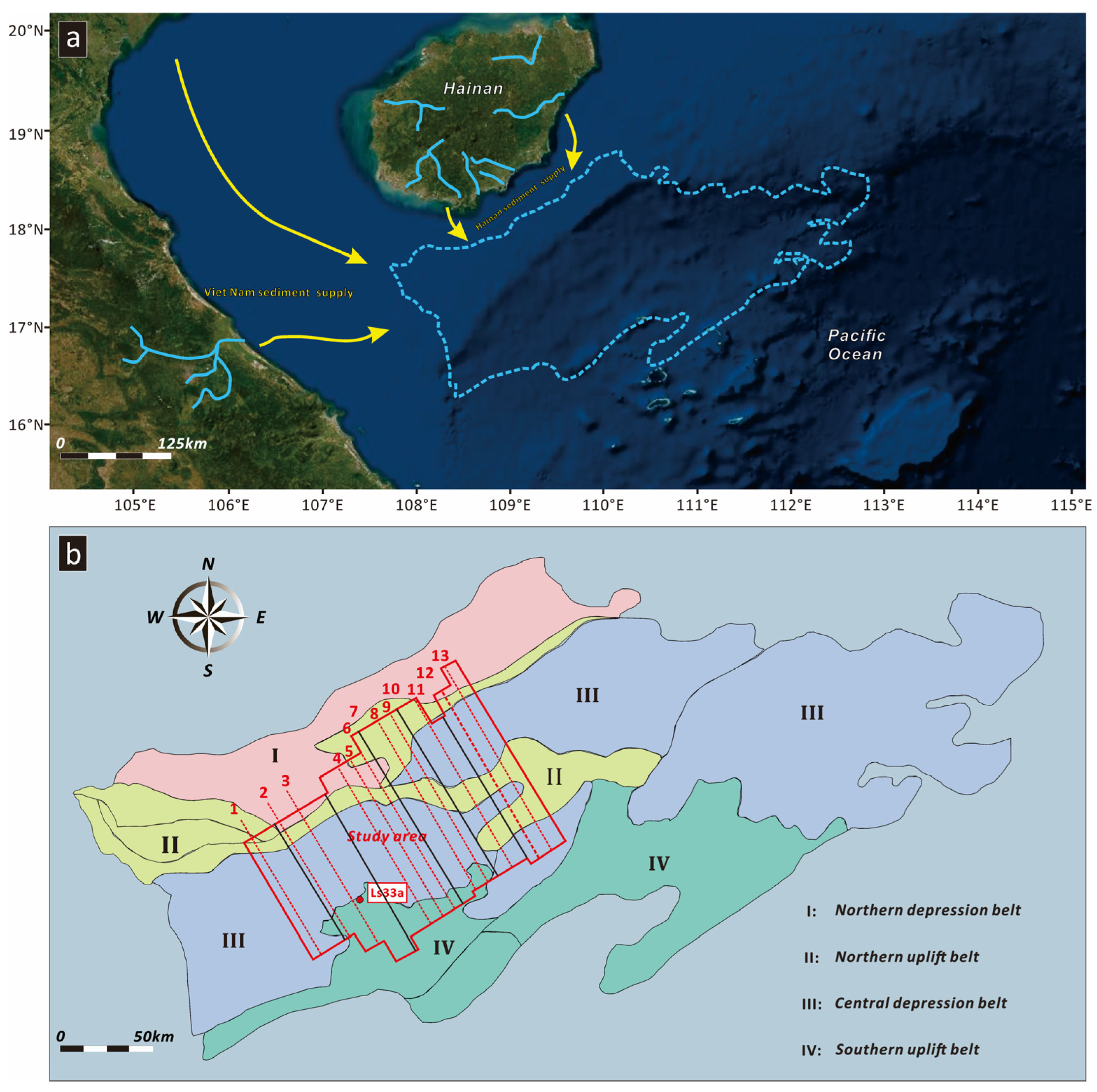
2. Geological Setting
3. Data and Potential Controlling Factors
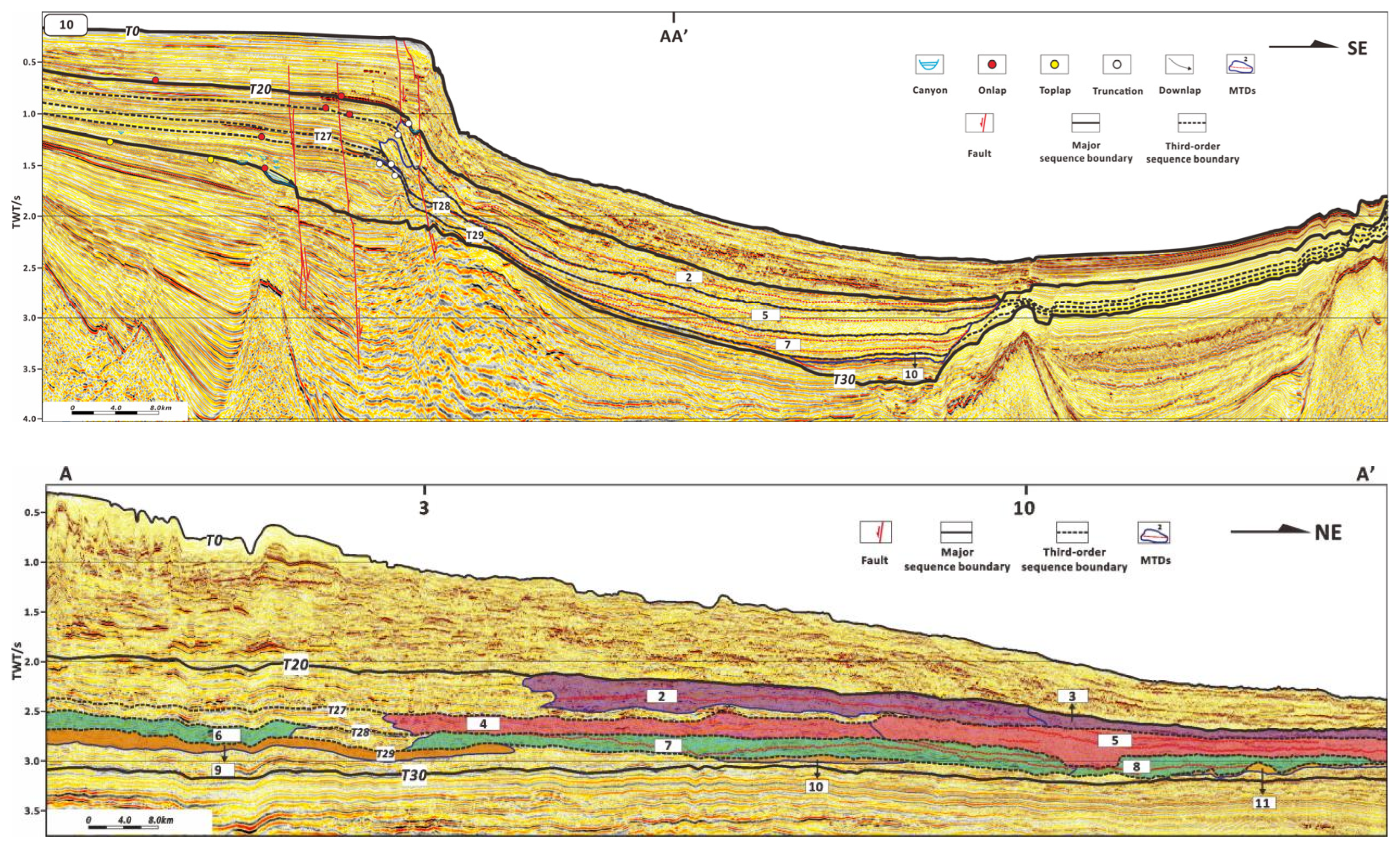
3.1. Data
3.2. Potential Controlling Factors of MTDs
- (1)
- Narrow and Negative Topography
- (2)
- Sedimentary factors
- (3)
- Climate factors
- (4)
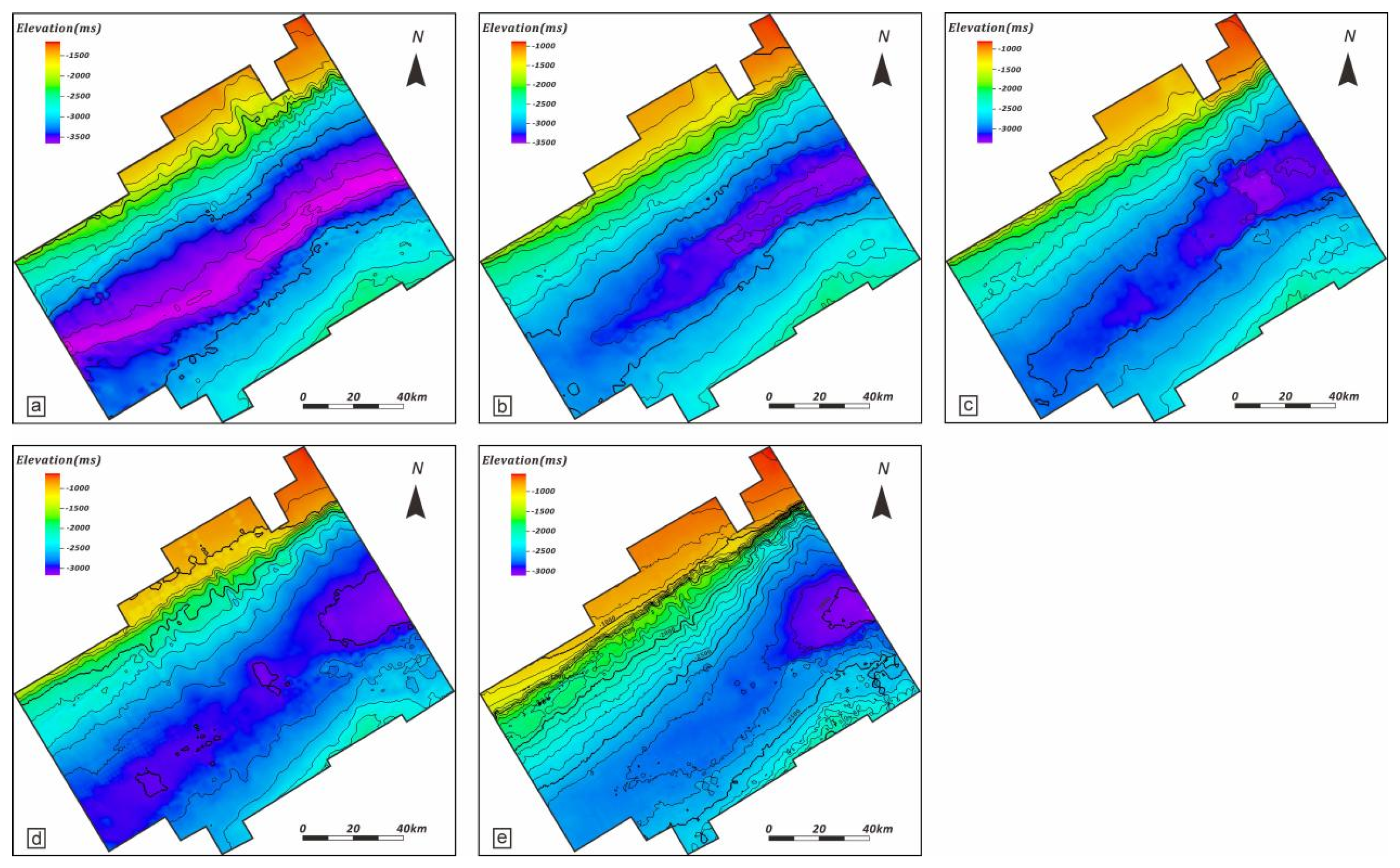
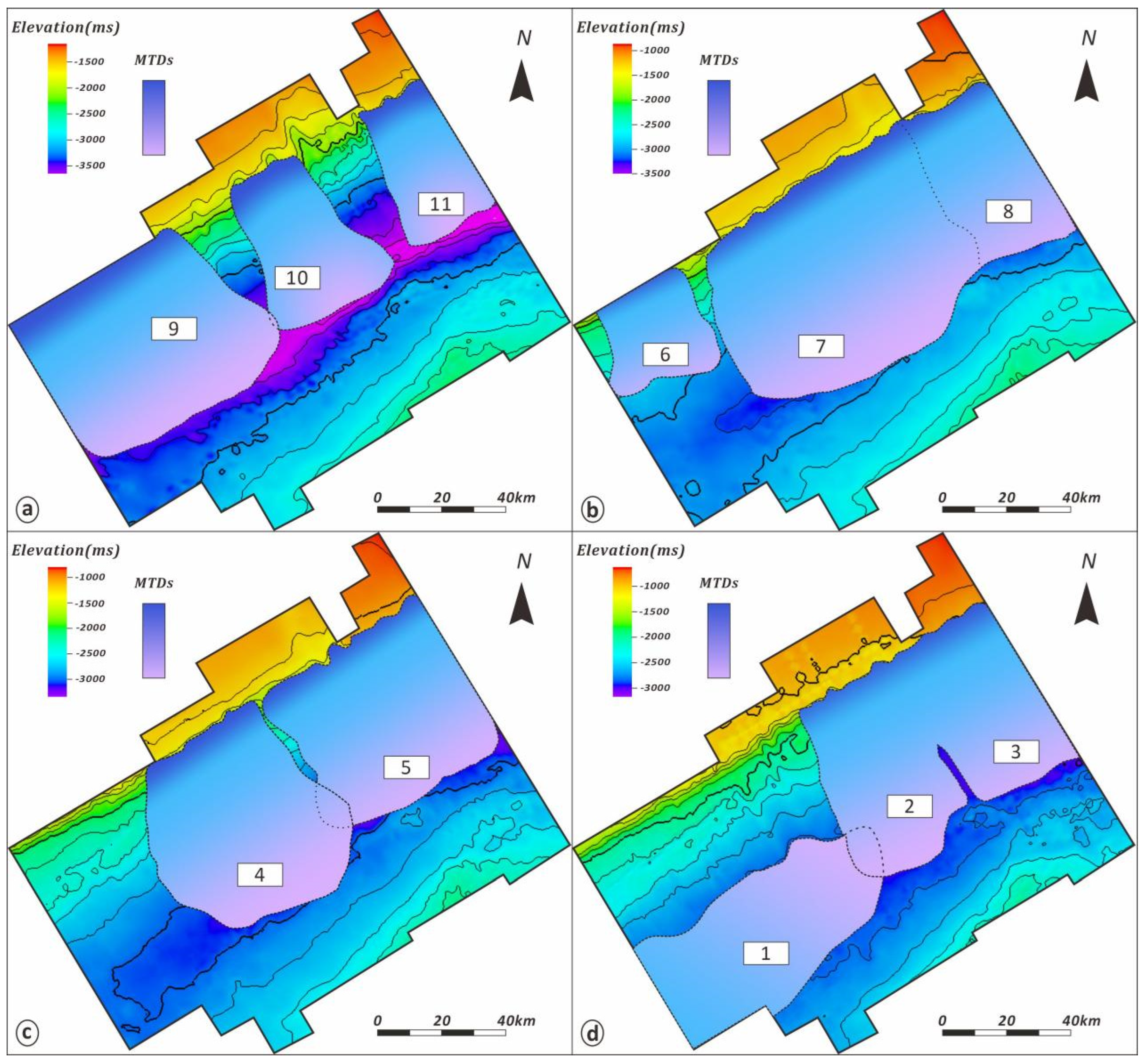
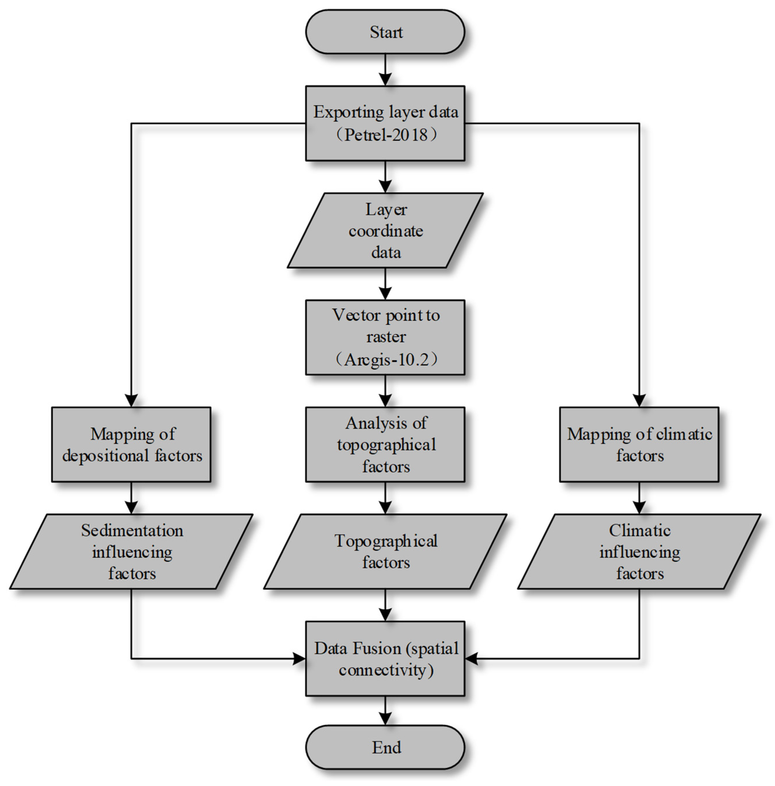
- Data mapping
4. Methodology
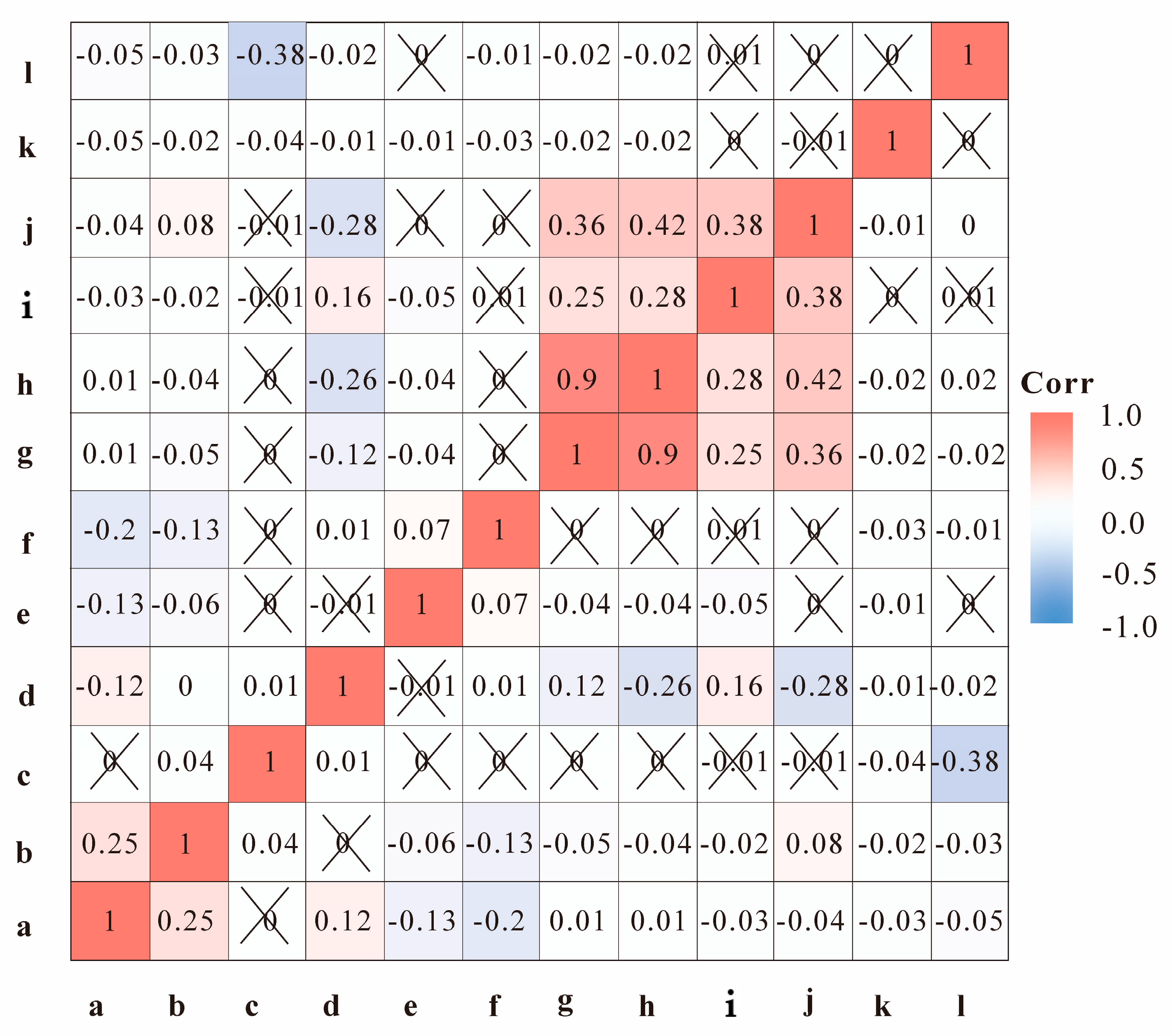
4.1. Correlation and Significance Checks
4.2. Recursive Feature Elimination
4.3. Random Forest Regression Algorithm
- (1)
- The bootstrap sampling technique is used in the random forest, and k new sample sets are randomly selected with put-back to build k decision trees; the samples that are not selected form k out-of-bag data.
- (2)
- A single decision tree is generated for each self-sample set.
- (3)
- Predict the data based on the results of the generated decision tree classifier to derive the category with the highest number of votes for the voting results of the decision tree.
4.4. Model Validation Methods
- (1)
- Cross-validation
- (2)
- Receiver Operating Characteristic (ROC)
5. The Main Controlling Factor for Triggering MTDs
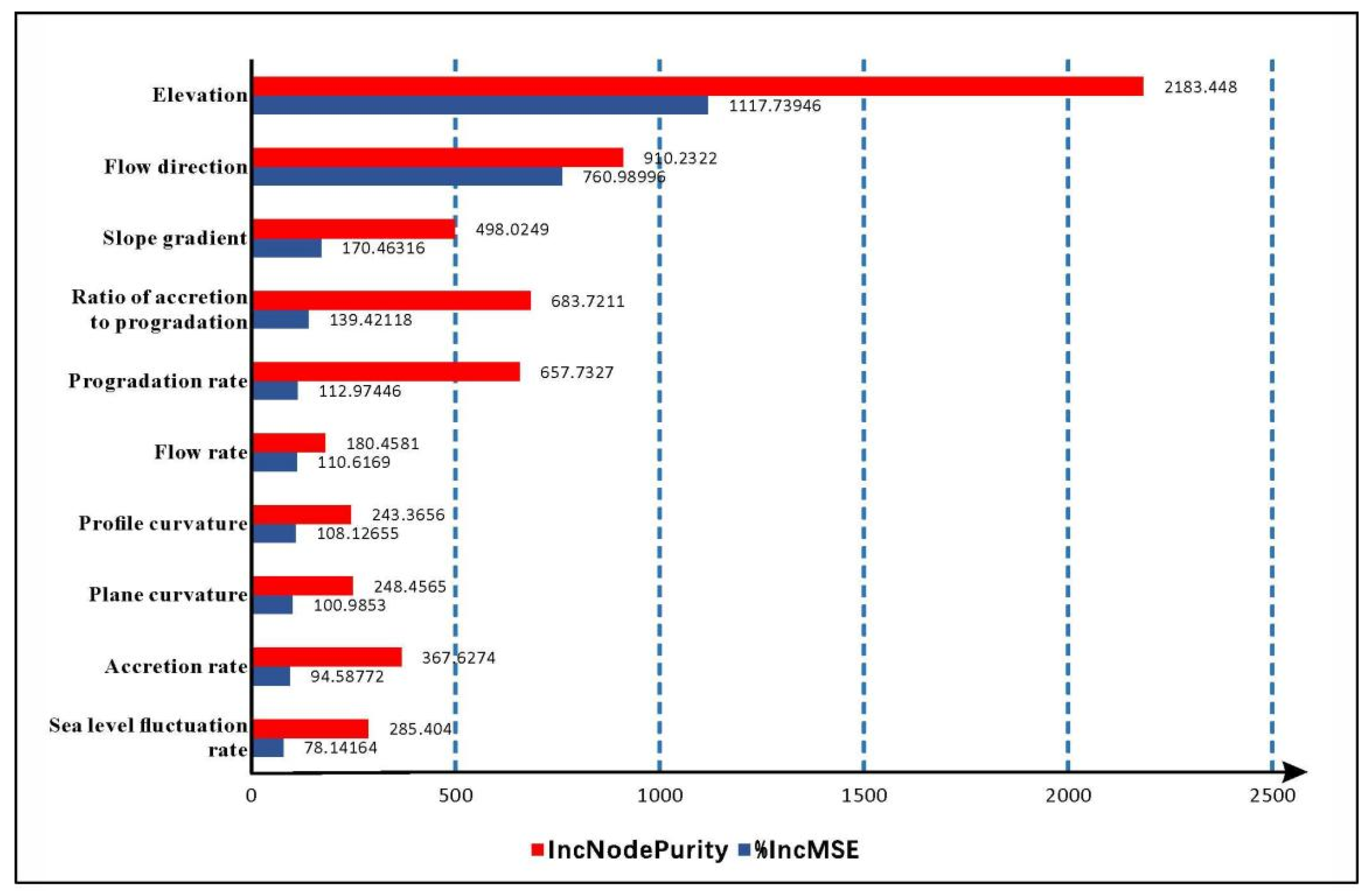
5.1. Screening of the Main Controlling Factors
5.2. MTD Occurrence Analysis
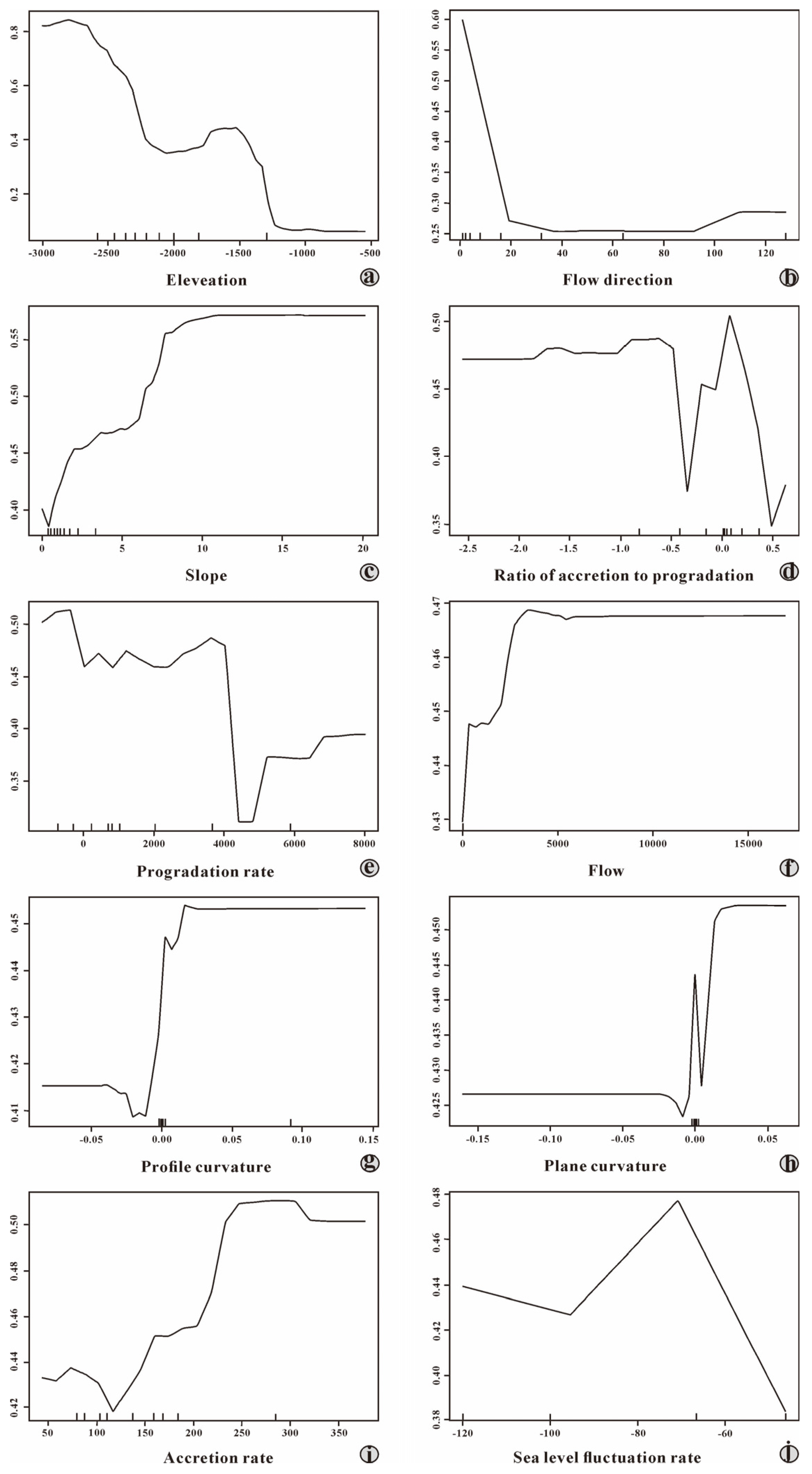
6. Partial Dependency Evaluation of Controlling Factors
7. Conclusions
Author Contributions
Funding
Institutional Review Board Statement
Informed Consent Statement
Data Availability Statement
Acknowledgments
Conflicts of Interest
References
- Tappin, D.R.; Watts, P.; McMurtry, G.M.; Lafoy, Y.; Matsumoto, T. The Sissano, Papua New Guinea tsunami of July 1998—Offshore evidence on the source mechanism. Mar. Geol. 2001, 175, 1–23. [Google Scholar] [CrossRef]
- Gaullier, V.; Loncke, L.; Droz, L.; Basile, C.; Maillard, A.; Patriat, M.; Carol, F. Slope instability on the French Guiana transform margin from swath-bathymetry and 3.5 kHz echograms. In Submarine Mass Movements and Their Consequences; Springer: Berlin/Heidelberg, Germany, 2010; pp. 569–579. [Google Scholar]
- Alves, T.M. Submarine slide blocks and associated soft-sediment deformation in deep-water basins: A review. Mar. Petrol. Geol. 2015, 67, 262–285. [Google Scholar] [CrossRef]
- Krastel, S.; Wynn, R.B.; Georgiopoulou, A.; Geersen, J.; Henrich, R.; Meyer, M.; Schwenk, T. Large-scale mass wasting on the Northwest African continental margin: Some general implications for mass wasting on passive continental margins. In Submarine Mass Movements and Their Consequences; Springer: Berlin/Heidelberg, Germany, 2012; Volume 31, pp. 189–199. [Google Scholar]
- Zhou, Q.; Li, X.; Zhou, H.; Liu, L.; Xu, Y.; Gao, S.; Ma, L. Characteristics and genetic analysis of submarine landslides in the northern slope of the South China Sea. Mar. Geophys. Res. 2019, 40, 303–314. [Google Scholar] [CrossRef]
- Maslin, M.; Owen, M.; Day, S.; Long, D. Linking continental-slope failures and climate change: Testing the clathrate gun hypothesis. Geology 2004, 32, 53–56. [Google Scholar] [CrossRef]
- Canals, M.; Lastras, G.; Urgeles, R.; Casamor, J.L.; Mienert, J.; Cattaneo, A.; De Batist, M.; Haflidason, H.; Imbo, Y.; Laberg, J.S.; et al. Slope failure dynamics and impacts from seafloor and shallow sub-seafloor geophysical data: Case studies from the COSTA project. Mar. Geol. 2004, 213, 9–72. [Google Scholar] [CrossRef]
- Weimer, P.; Slatt, R.; Bouroullec, R.; Fillon, R.; Pettingill, H.; Pranter, M.; Tari, G. Introduction to the petroleum geology of deepwater setting. Geology 2006, 32, 53–56. [Google Scholar]
- Moscardelli, L.; Wood, L. New classification system for mass transport complexes in offshore Trinidad. Basin Res. 2008, 20, 73–98. [Google Scholar] [CrossRef]
- Liapidevskii, V.Y.; Dutykh, D.; Gisclon, M. On the modelling of shallow turbidity flows. Adv. Water Resour. 2018, 113, 310–327. [Google Scholar] [CrossRef]
- Wu, S.G.; Qin, Z.L.; Wang, D.W.; Peng, X.C.; Wang, Z.J. Seismic characteristics and triggering mechanism analysis of mass transport deposits in the northern continental slope of the South China Sea. Chin. J. Geophys. 2011, 54, 3184–3195. [Google Scholar]
- He, Y.L. The Characteristics and Mechanism of Sediment Gravity Flow in Slope Area in Qiongdongnan Basin. Ph.D. Thesis, China University of Geosciences, Wuhan, China, 2012. [Google Scholar]
- Qin, Z.L. Sedimentary Process, Distribution and Mechanism of Mass Transport Deposits, the Slope Area of Northern South China Sea; Institute of Oceanology, Chinese Academy of Sciences: Qingdao, China, 2012. [Google Scholar]
- Moscardelli, L.; Wood, L.; Mann, P. Mass-transport complexes and associated processes in the offshore area of Trinidad and Venezuela. AAPG Bull. 2006, 90, 1059–1088. [Google Scholar] [CrossRef]
- Shanmugam, G. New Perspectives on Deep-Water Sandstones: Origin, Recognition, Initiation, and Reservoir Quality; Elsevier: Amsterdam, The Netherlands, 2012. [Google Scholar]
- Qin, Y.Q.; Wan, L.K.; Ji, Z.F.; Xu, H.L.; Ba, D. Progress of research on deep-water mass-transport deposits. Oil Gas Geol. 2018, 39, 140–152. [Google Scholar]
- Pirmez, C.; Marr, J.; Shipp, C.; Kopp, F. Observations and numerical modeling of debris flows in the Na Kika Basin, GulfofMexico. In Proceedings of the Offshore Technology Conference, Houston, TX, USA, 3–6 May 2004. [Google Scholar]
- Shipp, R.C.; Nott, J.A.; Newlin, J.A. Physical characteristics and impact of mass transport complexes on deepwater jetted conductors and suction anchor piles. In Proceedings of the Offshore Technology Conference, Houston, TX, USA, 3–6 May 2004. [Google Scholar]
- Meckel, L.D.; Angelatos, M.; Bonnie, J.; McGarva, R.; Almond, T.; Marshall, N.; Bourdon, L.; Aurisch, K. Reservoir characterization of sand-prone mass-trans-port deposits within slope canyons. In Mass-Transportdeposits in Deepwater Settings: SEPM Special Publication; Shipp, R.C., Weimer, P., Posamentier, H.W., Eds.; Tulsa: Claremore, OK, USA, 2011; Volume 96, pp. 391–421. [Google Scholar]
- Wang, D.W.; Wu, S.G.; Lu, F.L.; Wang, B.W. Mass transport deposits and its significance for oil & gas exploration in deep-water regions of South China Sea. J. China Univ. Pet. (Ed. Nat. Sci.) 2011, 35, 14–19. [Google Scholar]
- Alves, T.M.; Kurtev, K.; Moore, G.F.; Strasser, M. Assessing the internal character, reservoir potential, and seal competence of mass-transport deposits using seismic texture: A geophysical and petrophysical approach. AAPG Bull. 2014, 98, 793–824. [Google Scholar] [CrossRef]
- Carter, L. Submarine Cables and the Oceans: Connecting the World; UNEP/Earthprint: Nairobi, Kenya, 2010. [Google Scholar]
- Bardet, J.P.; Synolakis, C.E.; Davies, H.L.; Imamura, F.; Okal, E.A. Landslide tsunamis: Recent findings and research directions. Landslide Tsunamis Recent Find. Res. Dir. 2003, 160, 1793–1809. [Google Scholar]
- Ramadan, K.T.; Omar, M.A.; Allam, A.A. Modeling of tsunami generation and propagation under the effect of stochastic submarine landslides and slumps spreading in two orthogonal directions. Ocean Eng. 2014, 75, 90–111. [Google Scholar] [CrossRef]
- Feng, X.; Yin, B.; Gao, S.; Wang, P.; Bai, T.; Yang, D. Assessment of tsunami hazard for coastal areas of Shandong Province, China. Appl. Ocean Res. 2017, 62, 37–48. [Google Scholar] [CrossRef]
- Sassa, S.; Takagawa, T. Liquefied gravity flow-induced tsunami: First evidence and comparison from the 2018 Indonesia Sulawesi earthquake and tsunami disasters. Landslides 2019, 16, 195–200. [Google Scholar] [CrossRef]
- Locat, J.; Ten Brink, U.S.; Chaytor, J.D. The block composite submarine landslide, southern New England slope, USA: A morphological analysis. In Submarine Mass Movements and Their Consequences; Springer: Berlin/Heidelberg, Germany, 2010; Volume 28, pp. 267–277. [Google Scholar]
- Ma, L.W.; Wu, S.G.; Liu, Y.R.; Sun, J.; Min, O.Y.; Li, Q.P.; Qin, Y.P.; Wang, D.W. Slope Instability Analysis of the Qiongdongnan Basin in the Northern Part of the South China Sea: Implications for the Risk Evaluation of Deepwater Drilling. J. Ocean Univ 2023, 22, 393–409. [Google Scholar] [CrossRef]
- Masson, D.G.; Harbitz, C.B.; Wynn, R.B.; Pedersen, G.; Løvholt, F. Submarine landslides: Processes, triggers and hazard prediction. Philos. Trans. R. Soc. A Math. Phys. Eng. Sci. 2006, 364, 2009–2039. [Google Scholar] [CrossRef]
- Talling, P.J.; Clare, M.; Urlaub, M.; Pope, E.; Hunt, J.E.; Watt SF, L. Large submarine landslides on continental slopes: Geohazards, methane release, and climate change. Oceanography 2014, 27, 32–45. [Google Scholar] [CrossRef]
- Kremer, K.; Usman, M.O.; Satoguchi, Y.; Nagahashi, Y.; Vadakkepuliyambatta, S.; Panieri, G.; Strasser, M. Possible climate preconditioning on submarine landslides along a convergent margin, Nankai Trough (NE Pacific). Prog. Earth. Planet. Sci. 2017, 4, 20. [Google Scholar] [CrossRef]
- Rodríguez-Ochoa, R.; Nadim, F.; Hicks, M.A. Influence of weak layers on seismic stability of submarine slopes. Mar. Pet. Geol. 2015, 65, 247–268. [Google Scholar] [CrossRef]
- Nian, T.K.; Guo, X.S.; Zheng, D.F.; Xiu, Z.X.; Jiang, Z.B. Susceptibility assessment of regional submarine landslides triggered by seismic actions. Appl. Ocean Res. 2019, 93, 101964. [Google Scholar] [CrossRef]
- Urlaub, M.; Zervos, A.; Talling, P.J.; Masson, D.G.; Clayton, C.I. How do∼2° slopes fail in areas of slow sedimentation? A sensitivity study on the influence of accumulation rate and permeability on submarine slope stability. In Submarine Mass Movements and Their Consequences; Springer: Berlin/Heidelberg, Germany, 2012; pp. 277–287. [Google Scholar]
- Liu, F.; Tan, L.; Crosta, G.; Huang, Y. Spatiotemporal destabilization modes of upper continental slopes undergoing hydrate dissociation. Eng. Geol. 2020, 264, 105286. [Google Scholar] [CrossRef]
- Yang, S.; Choi, J.C.; Vanneste, M.; Kvalstad, T. Effects of gas hydrates dissociation on clays and submarine slope stability. Bull. Eng. Geol. Environ. 2018, 77, 941–952. [Google Scholar] [CrossRef]
- Llopart, J.; Urgeles, R.; Camerlenghi, A.; Lucchi, R.G.; Mol, B.D.; Rebesco, M.; Pedrosa, M.T. Slope instability of glaciated continental margins: Constraints from permeability-compressibility tests and hydrogeological modeling off Storfjorden, NW Barents Sea. In Submarine Mass Movements and Their Consequences; Springer: Berlin/Heidelberg, Germany, 2014; pp. 95–104. [Google Scholar]
- Gales, J.A.; Mckay, R.M.; De Santis, L.; Rebesco, M.; Laberg, J.S.; Shevenell, A.E.; Harwood, D.; Leckie, R.M.; Kulhanek, D.K.; King, M.; et al. Climate-controlled submarine landslides on the Antarctic continental margin. Nat. Commun. 2023, 14, 2714. [Google Scholar] [CrossRef]
- Bessette-Kirton, E.K.; Coe, J.A.; Schulz, W.H.; Cerovski-Darriau, C.; Einbund, M.M. Mobility characteristics of debris slides and flows triggered by Hurricane Maria in Puerto Rico. Landslides 2020, 17, 2795–2809. [Google Scholar] [CrossRef]
- Zhu, H.; Yang, X.; Liu, K.; Zhou, X. Seismic-based sediment provenance analysis in continental lacustrine rift basins: An example from the Bohai Bay Basin, China. AAPG Bull. 2014, 98, 1995–2018. [Google Scholar] [CrossRef]
- Zhu, W.L. Discrepancy tectonic evolution and petroleum exploration in China offshore Cenozoic Basins. Earth Sci. Front. 2015, 22, 88–101. [Google Scholar]
- Zhu, W.L.; Zhang, G.C.; Gao, L. Geological characteristics and exploration objectives of hydrocarbons in the northern continental margin basin of South China Sea. Acta Pet. Sin. 2008, 29, 1–9. [Google Scholar]
- Clift, P.D.; Sun, Z. The sedimentary and tectonic evolution of the Yinggehai-Song Hong basin and the southern Hainan margin, South China Sea: Implications for Tibetan uplift and monsoon intensification. J. Geophys. Res. Solid Earth 2006, 111, B6. [Google Scholar] [CrossRef]
- Leloup, P.H.; Lacassin, R.; Tapponnier, P.; Schärer, U.; Zhong, D.; Liu, X.; Trinh, P.T. The Ailao Shan-Red river shear zone (Yunnan, China), tertiary transform boundary of Indochina. Tectonophysics 1995, 251, 3–84. [Google Scholar] [CrossRef]
- Du, T.J. Sequence Stratigraphic and Deep Water Sedimentaiy Characteristic in the Qingdongnan Basin. Master’s Thesis, Ocean University of China, Qingdao, China, 2013. [Google Scholar]
- Liu, X.F.; Sun, Z.P.; Liu, X.Y.; Liu, D.S.; Zhai, S.K.; Long, H.Y.; Jiang, L.J.; Bi, D.J. Chronostratigraphic Framework based on Micro-paleontological Data from Drilling LS33a in Deep Water Area of Northern South China Sea. Acta Sedimentol. Sin. 2018, 36, 890–902. [Google Scholar] [CrossRef]
- Li, W.; Alves, T.M.; Rebesco, M.; Sun, J.; Li, J.; Li, S.; Wu, S. The Baiyun Slide Complex, South China Sea: A modern example of slope instability controlling submarine-channel incision on continental slopes. Mar. Pet. Geol. 2020, 114, 104231. [Google Scholar] [CrossRef]
- Zhang, K.; Song, H.; Sun, S.; Gao, J. Distribution and genesis of submarine landslides in the northeastern South China Sea. Geol. J. 2021, 56, 1187–1201. [Google Scholar] [CrossRef]
- Gamboa, D.; Omira, R.; Terrinha, P. Spatial and morphometric relationships of submarine landslides offshore west and southwest Iberia. Landslides 2022, 19, 387–405. [Google Scholar] [CrossRef]
- Yang, S.L.; Solheim, A.; Forsberg, C.F.; Kvalstad, T.; Feng, X.L.; Li, A.L.; Urgeles, R. Geotechnical properties of river-fed sediments compared with glacier-fed sediments. Mar. Georesources Geotechnol. 2009, 27, 281–295. [Google Scholar] [CrossRef]
- Lucchi, R.G.; Pedrosa, M.T.; Camerlenghi, A.; Urgeles, R.; De Mol, B.; Rebesco, M. Recent submarine landslides on the continental slope of Storfjorden and Kveithola Trough-Mouth Fans (north west Barents Sea). In Submarine Mass Movements and Their Consequences; Springer: Berlin/Heidelberg, Germany, 2012; Volume 31, pp. 735–745. [Google Scholar]
- Stoecklin, A.; Friedli, B.; Puzrin, A.M. Sedimentation as a control for large submarine landslides: Mechanical modeling and analysis of the Santa Barbara Basin. J. Geophys. Res. Solid Earth 2017, 122, 8645–8663. [Google Scholar] [CrossRef]
- Helland-Hansen, W.; Hampson, G.J. Trajectory analysis: Concepts and applications. Basin Res. 2009, 21, 454–483. [Google Scholar] [CrossRef]
- Joh, M.H.; Yoo, D.G. Plio-Quaternary seismic stratigraphy and depositional history on the southern Ulleung Basin, East Sea. Sea: J. Korean Soc. Oceanogr. 2009, 14, 90–101. [Google Scholar]
- Yi, Y.M.; Yoo, D.G.; Kang, N.K.; Yi, B.Y. Distribution and origin of quaternary mass transport deposit in the Ulleung Basin, East Sea. Geophys. Geophys. Explor. 2014, 17, 74–87. [Google Scholar] [CrossRef]
- Lisiecki, L.E.; Raymo, M.E. Correction to “A Pliocene-Pleistocene stack of 57 globally distributed benthic δ18O records”. Paleoceanogr. Paleoclimatology 2005, 20, 1–17. [Google Scholar] [CrossRef]
- Revell, L.J.; Harrison, A.S. PCCA: A program for phylogenetic canonical correlation analysis. Bioinformatics 2008, 24, 1018–1020. [Google Scholar] [CrossRef] [PubMed]
- Melnykov, A.V.; Hall, K.B. Revival of high-order fluorescence correlation analysis: Generalized theory and biochemical applications. J. Phys. Chem. B 2009, 113, 15629–15638. [Google Scholar] [CrossRef]
- Witt, A.; Malamud, B.D.; Rossi, M.; Guzzetti, F.; Peruccacci, S. Temporal correlations and clustering of landslides. Earth Surf. Process. Landf. 2010, 35, 1138–1156. [Google Scholar] [CrossRef]
- Strauss, L.G.; Koczan, D.; Seiz, M.; Tuettenberg, J.; Schmieder, K.; Pan, L.; Dimitrakopoulou-Strauss, A. Correlation of the Ga-68-bombesin analog Ga-68-BZH3 with receptors expression in gliomas as measured by quantitative dynamic positron emission tomography (dPET) and gene arrays. Mol. Imaging Biol. 2012, 14, 376–383. [Google Scholar] [CrossRef]
- Geitner, R.; Fritzsch, R.; Popp, J.; Bocklitz, T.W. corr2D-implementation of two-dimensional correlation analysis in R. arXiv 2018, arXiv:1808.00685. [Google Scholar] [CrossRef]
- Guyon, I.; Weston, J.; Barnhill, S.; Vapnik, V. Gene Selection for Cancer Classification using Support Vector Machines. Mach. Learn. 2002, 46, 389–422. [Google Scholar] [CrossRef]
- Naghavi, H.; Fallah, A.; Shataee, S.; Latifi, H.; Soosani, J.; Ramezani, H.; Conrad, C. Canopy cover estimation across semi-Mediterranean woodlands: Application of high-resolution earth observation data. J. Appl. Remote Sens. 2014, 8, 083524. [Google Scholar] [CrossRef]
- Bachofer, F.; Quénéhervé, G.; Hochschild, V.; Maerker, M. Multisensoral topsoil mapping in the semiarid Lake Manyara region, northern Tanzania. Remote Sens. 2015, 7, 9563–9586. [Google Scholar] [CrossRef]
- Sorenson, P.T.; Kiss, J.; Bedard-Haughn, A.K.; Shirtliffe, S. Multi-Horizon Predictive Soil Mapping of Historical Soil Properties Using Remote Sensing Imagery. Remote Sens. 2022, 14, 5803. [Google Scholar] [CrossRef]
- Breiman, L. Bagging predictors. Mach. Learn. 1996, 24, 123–140. [Google Scholar] [CrossRef]
- Cutler, A.; Stevens, J.R. random forests for microarrays. Methods Enzymol. 2006, 411, 422–432. [Google Scholar] [PubMed]
- Gholinejad, S.; Naeini, A.A.; Amiri-Simkooei, A. Robust particle swarm optimization of RFMs for high-resolution satellite images based on k-fold cross-validation. IEEE J. Sel. Top. Appl. Earth Obs. Remote Sens. 2018, 12, 2594–2599. [Google Scholar] [CrossRef]
- Al-Mukhtar:, M. Random forest, support vector machine, and neural networks to modeling suspended sediment in Tigris River-Baghdad. Environ. Monit. Assess. 2019, 191, 673. [Google Scholar] [CrossRef]
- Leshowitz, B. Comparison of ROC Curves from One- and Two-Interval Rating-Scale Procedures. J. Acoust. Soc. Am. 1969, 46, 399–402. [Google Scholar] [CrossRef]
- Cukur, D.; Kim, S.-P.; Kong, G.-S.; Bahk, J.-J.; Horozal, S.; Um, I.-K.; Lee, G.-S.; Chang, T.-S.; Ha, H.-J.; Völker, D.; et al. Geophysical evidence and inferred triggering factors of submarine landslides on the western continental margin of the Ulleung Basin, East Sea. Geo-Mar Lett. 2016, 36, 425–444. [Google Scholar] [CrossRef]
- Gauchery, T.; Rovere, M.; Pellegrini, C.C.; Cattaneo, A.; Campiani, E.; Trincardi, F. Factors controlling margin instability during the Plio-Quaternary in the Gela Basin (Strait of Sicily, Mediterranean Sea). Mar. Pet. Geol. 2021, 123, 104767. [Google Scholar] [CrossRef]
- Wang, W.W.; Wang, D.W.; Wu, S.G.; Völker, D.; Zeng, H.L.; Cai, G.Q.; Li, Q.P. Submarine landslides on the north continental slope of the South China Sea. J. Ocean Univ. China 2018, 17, 83–100. [Google Scholar] [CrossRef]
- Yue, C.; Zhao, X.M.; Ge, J.W.; Ma, C.; Liao, J.; Song, P.; Fang, X.Y.; Fan, T.E. Evolution and Main Controlling Factors of Continental Shelf-edge Trajectory in Yinggehai Formation, Qiongdongnan Basin. Acta Sedimentol. Sin. 2023, 41, 110–125. [Google Scholar] [CrossRef]
- Rothwell, R.G.; Thomson, J.; Kähler, G. Low-sea-level emplacement of a very large late Pleistocene “megaturbidite” in the Western Mediterranean Sea. Nature 1998, 392, 377–380. [Google Scholar] [CrossRef]


| Sequence | Number | Locations in the Study Area | Length (km) | Width (km) |
|---|---|---|---|---|
| SQ4 (T27-T20) | 1 | Southwest | 89.76 | 33.18 |
| 2 | North central | 64.27 | 37.50 | |
| 3 | Northeast | 60.69 | 36.62 | |
| SQ3 (T28-T27) | 4 | North central | 66.09 | 49.34 |
| 5 | Northeast | 56.09 | 63.26 | |
| SQ2 (T29-T28) | 6 | Northwest | 35.72 | 28.51 |
| 7 | Central | 66.72 | 78.12 | |
| 8 | Central–Northeast | 58.48 | 48.06 | |
| SQ1 (T30-T29) | 9 | Northwest | 57.71 | 75.53 |
| 10 | North central | 53.22 | 31.44 | |
| 11 | Northeast | 48.68 | 27.83 |
| Factor Category | Variables | Data Type | Number Range | Unit |
|---|---|---|---|---|
| Topographic factors | Elevation | Continuous | [−2552.011~−54.627] | m |
| Slope | Continuous | [0~17.603] | ° | |
| Slope direction | Continuous | [1, 2, 3, 4, 5, 6, 7, 8] | - | |
| Profile curvature | Continuous | [−0.085~0.141] | - | |
| Plane curvature | Continuous | [−0.161~0.03] | - | |
| Flow direction | Categorical | [1, 2, 4, 8, 16, 32, 64, 128] | - | |
| Flow | Continuous | [0, 1, 2~16,970] | - | |
| Sedimentary factors | Accretion rate | Continuous | [43.801~377.153] | m/Ma |
| Progradation rate | Continuous | [−1175~8.13.889] | m/Ma | |
| Ratio of accretion to progradation | Continuous | [−2.557~0.628] | - | |
| Sediment fluxes | Continuous | [−348.101~1632.94] | m2/Ma | |
| Climatic factors | Sea level fluctuation rate | Continuous | [−120~−46.15] | m/Ma |
| Variables | Serial Number | RMSE | Rsquared | MAE | RMSESD | RsquaredSD | MAESD | Selected |
|---|---|---|---|---|---|---|---|---|
| Elevation | 1 | 0.5129 | 0.0869 | 0.3935 | 0.0045 | 0.0084 | 0.0056 | √ |
| Slope | 2 | 0.4349 | 0.2462 | 0.3451 | 0.0362 | 0.1086 | 0.0374 | √ |
| Progradation rate | 3 | 0.3105 | 0.6152 | 0.2205 | 0.0125 | 0.0312 | 0.0175 | √ |
| Ratio of accretion to progradation | 4 | 0.3094 | 0.6254 | 0.2298 | 0.0046 | 0.0132 | 0.0031 | √ |
| Flow | 5 | 0.3111 | 0.6278 | 0.2393 | 0.0044 | 0.0127 | 0.0034 | √ |
| Profile curvature | 6 | 0.2873 | 0.6695 | 0.1893 | 0.0074 | 0.0173 | 0.0069 | √ |
| Accretion rate | 7 | 0.2881 | 0.6703 | 0.1958 | 0.0054 | 0.0131 | 0.0039 | √ |
| Plane curvature | 8 | 0.2879 | 0.6730 | 0.2001 | 0.0048 | 0.0115 | 0.0040 | √ |
| Sea level fluctuation rate | 9 | 0.2374 | 0.7698 | 0.1357 | 0.0349 | 0.0683 | 0.0374 | √ |
| Flow direction | 10 | 0.2090 | 0.8253 | 0.1082 | 0.0049 | 0.0084 | 0.0025 | √ |
| Slope direction | 11 | 0.2094 | 0.8249 | 0.1098 | 0.0051 | 0.0087 | 0.0030 |
Disclaimer/Publisher’s Note: The statements, opinions and data contained in all publications are solely those of the individual author(s) and contributor(s) and not of MDPI and/or the editor(s). MDPI and/or the editor(s) disclaim responsibility for any injury to people or property resulting from any ideas, methods, instructions or products referred to in the content. |
© 2024 by the authors. Licensee MDPI, Basel, Switzerland. This article is an open access article distributed under the terms and conditions of the Creative Commons Attribution (CC BY) license (https://creativecommons.org/licenses/by/4.0/).
Share and Cite
Ge, J.; Zhao, X.; Fan, Q.; Pang, W.; Yue, C.; Chen, Y. The Controlling Factors and Prediction of Deep-Water Mass Transport Deposits in the Pliocene Qiongdongnan Basin, South China Sea. J. Mar. Sci. Eng. 2024, 12, 2115. https://doi.org/10.3390/jmse12122115
Ge J, Zhao X, Fan Q, Pang W, Yue C, Chen Y. The Controlling Factors and Prediction of Deep-Water Mass Transport Deposits in the Pliocene Qiongdongnan Basin, South China Sea. Journal of Marine Science and Engineering. 2024; 12(12):2115. https://doi.org/10.3390/jmse12122115
Chicago/Turabian StyleGe, Jiawang, Xiaoming Zhao, Qi Fan, Weixin Pang, Chong Yue, and Yueyao Chen. 2024. "The Controlling Factors and Prediction of Deep-Water Mass Transport Deposits in the Pliocene Qiongdongnan Basin, South China Sea" Journal of Marine Science and Engineering 12, no. 12: 2115. https://doi.org/10.3390/jmse12122115
APA StyleGe, J., Zhao, X., Fan, Q., Pang, W., Yue, C., & Chen, Y. (2024). The Controlling Factors and Prediction of Deep-Water Mass Transport Deposits in the Pliocene Qiongdongnan Basin, South China Sea. Journal of Marine Science and Engineering, 12(12), 2115. https://doi.org/10.3390/jmse12122115