
Incorporating Non-Equlibrium Ripple Dynamics into Bed Stress Estimates Under Combined Wave and Current Forcing

 , , and
Abstract
:1. Introduction
2. Model Equations
2.1. Wave–Current Interaction
2.2. Bedform Geometry Predictors
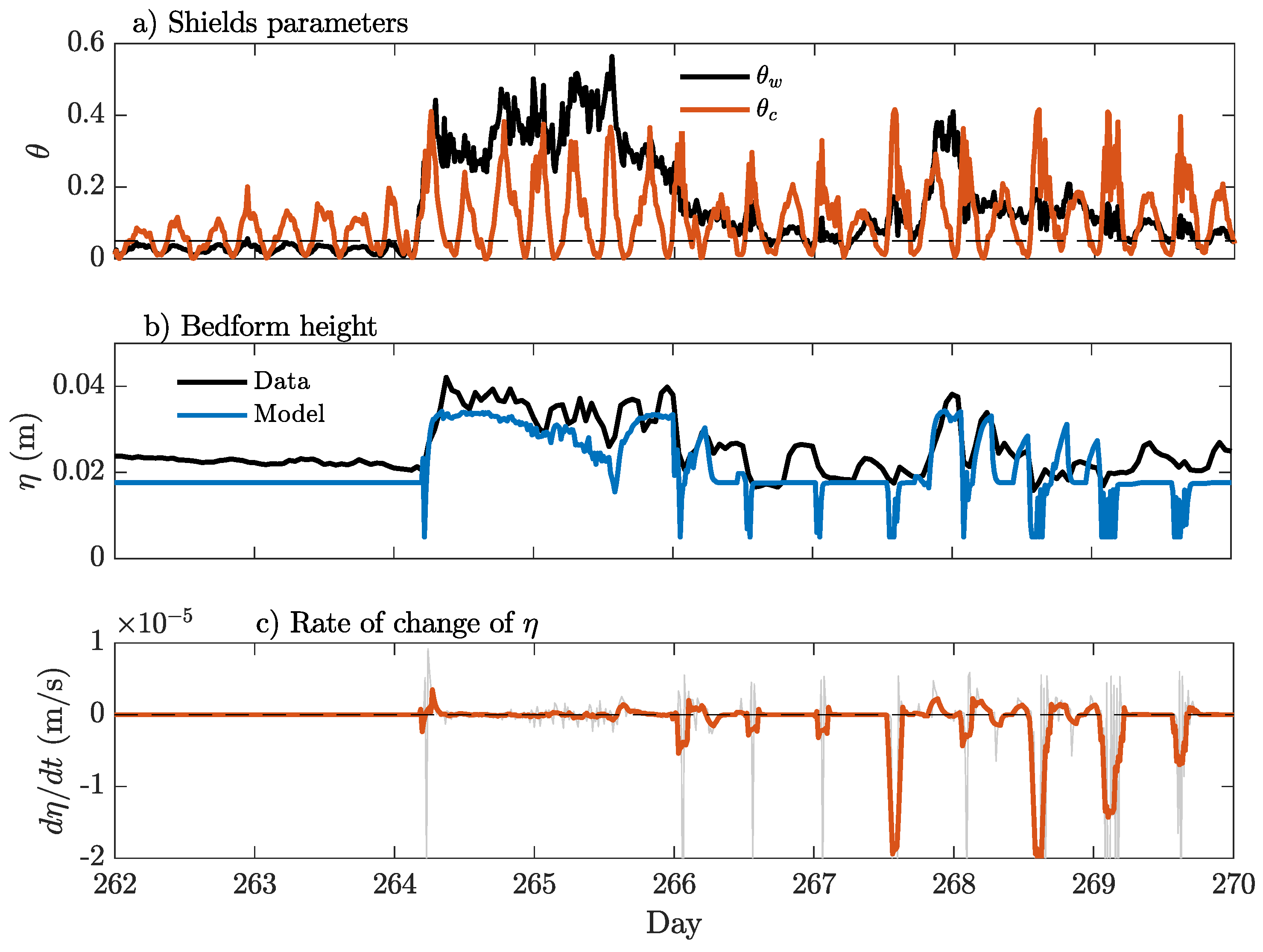
2.3. Prediction of Time-Evolving Ripple Dynamics
3. Methods
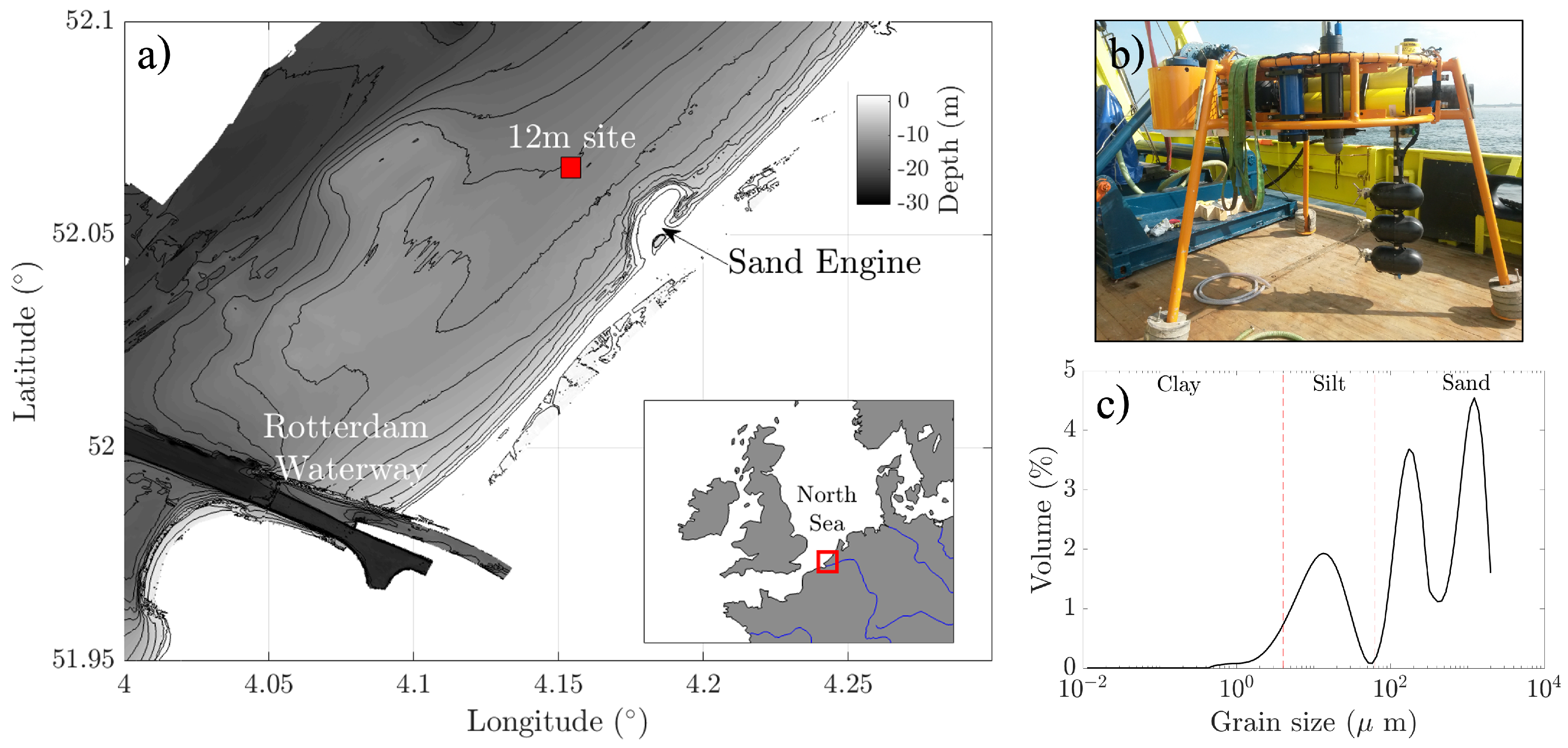
3.1. Data Collection
3.2. Data Processing
3.2.1. Near-Bottom Currents, Reynolds Stresses and Turbulent Fluxes
3.2.2. Wave Parameters
4. Results
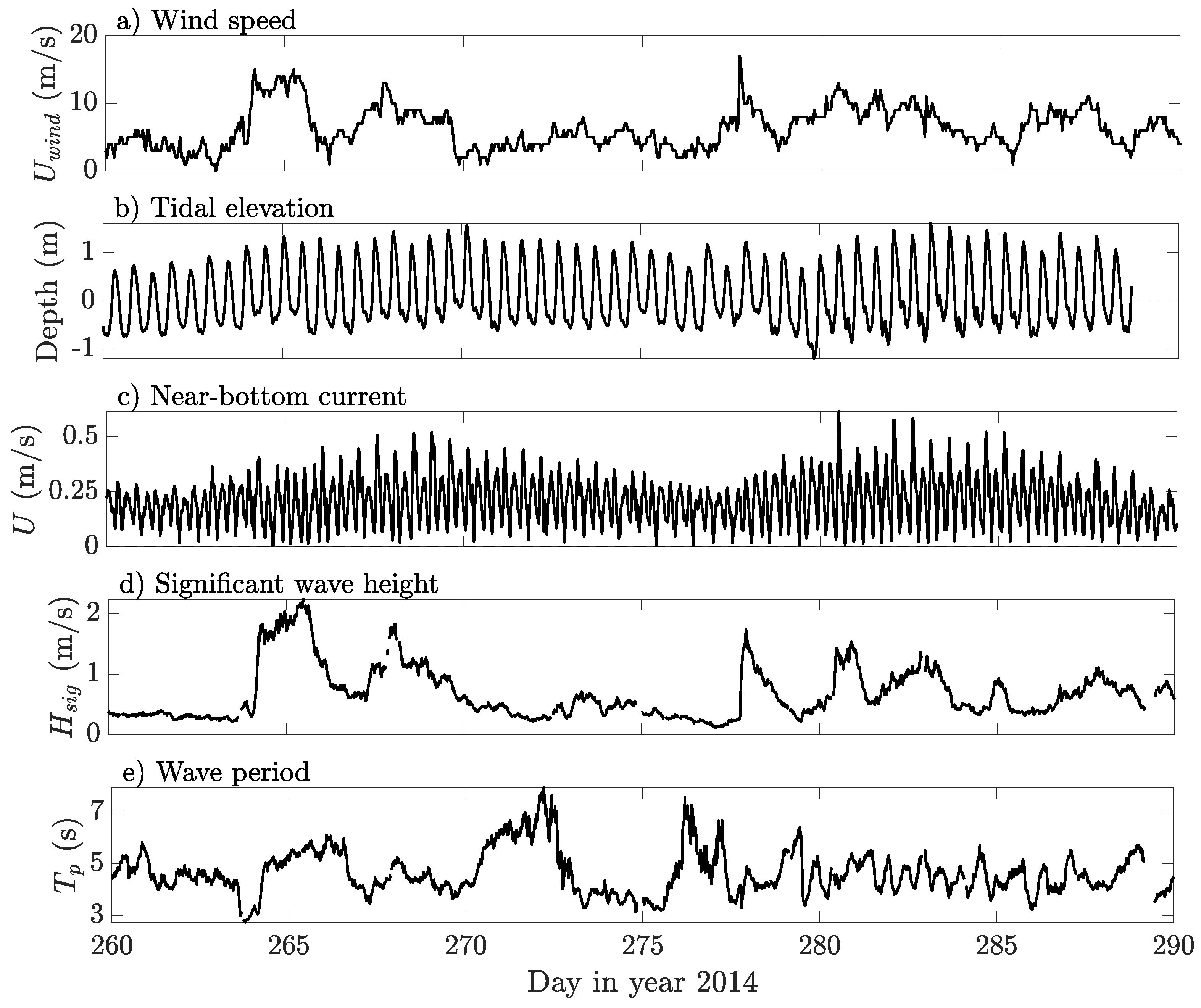
4.1. Experimental Conditions
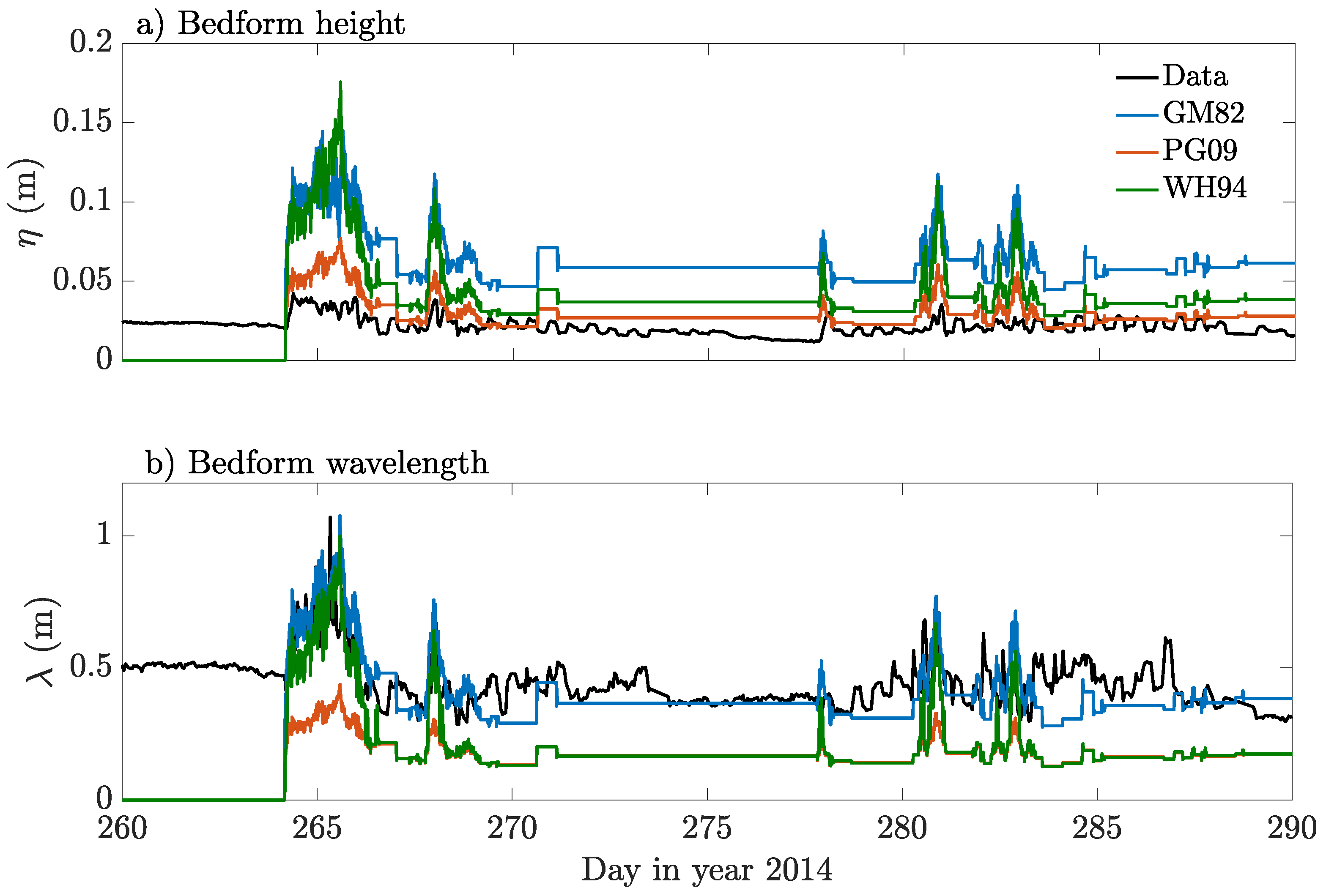
4.2. Bedforms
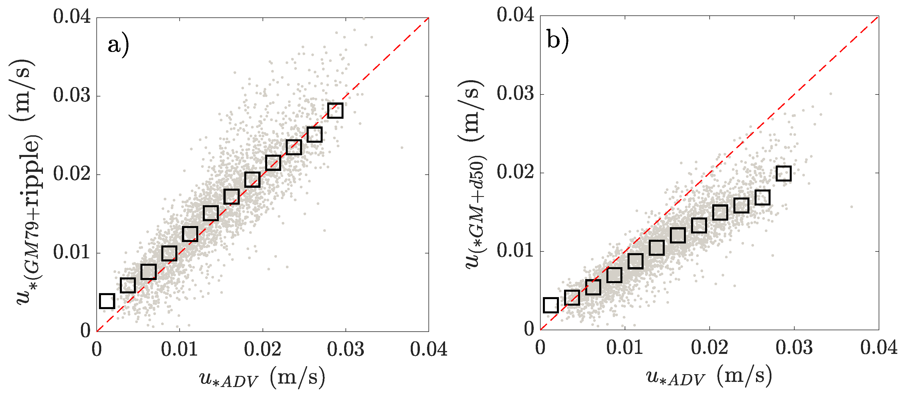
4.3. Bed Stress
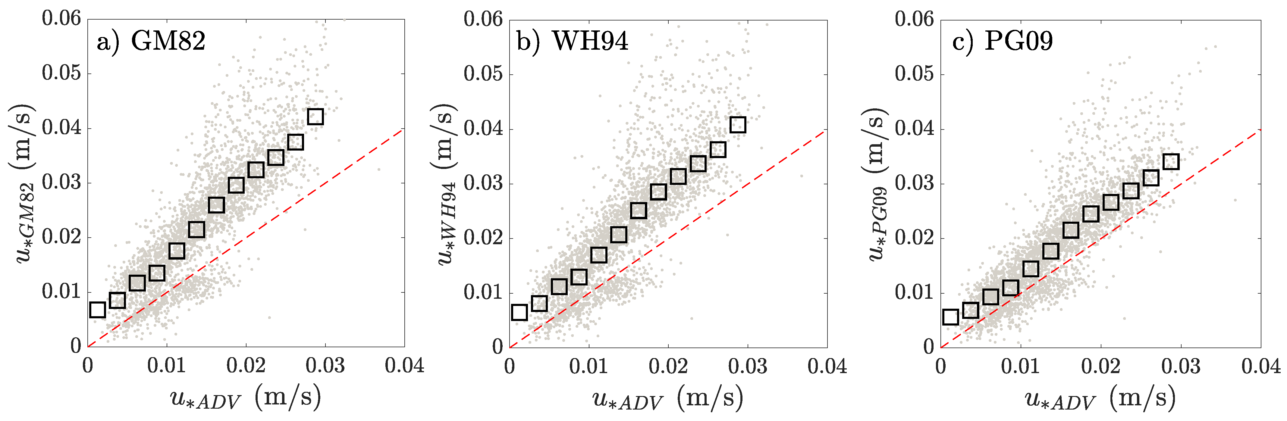
4.3.1. Measured Bedforms Versus Flat Bottom
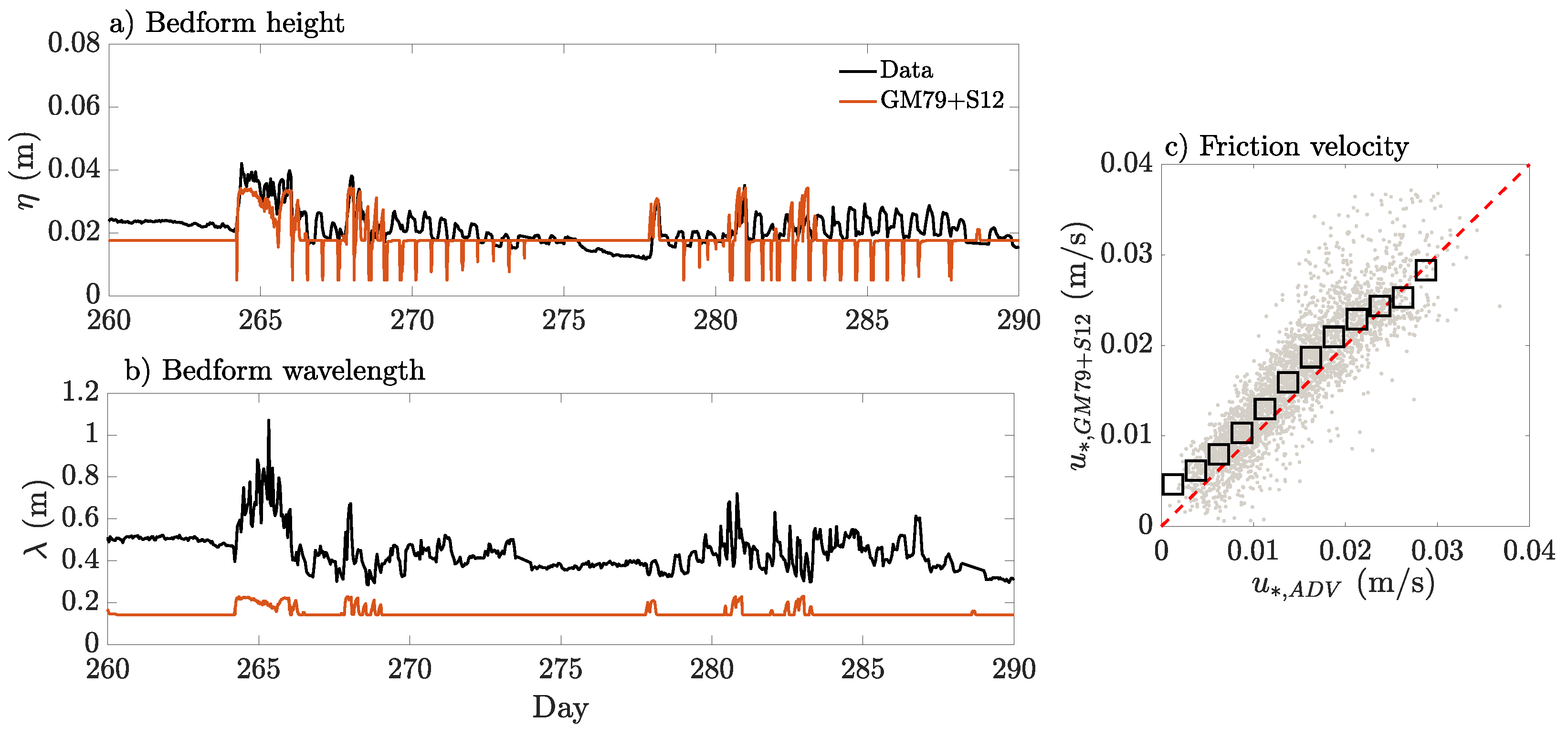
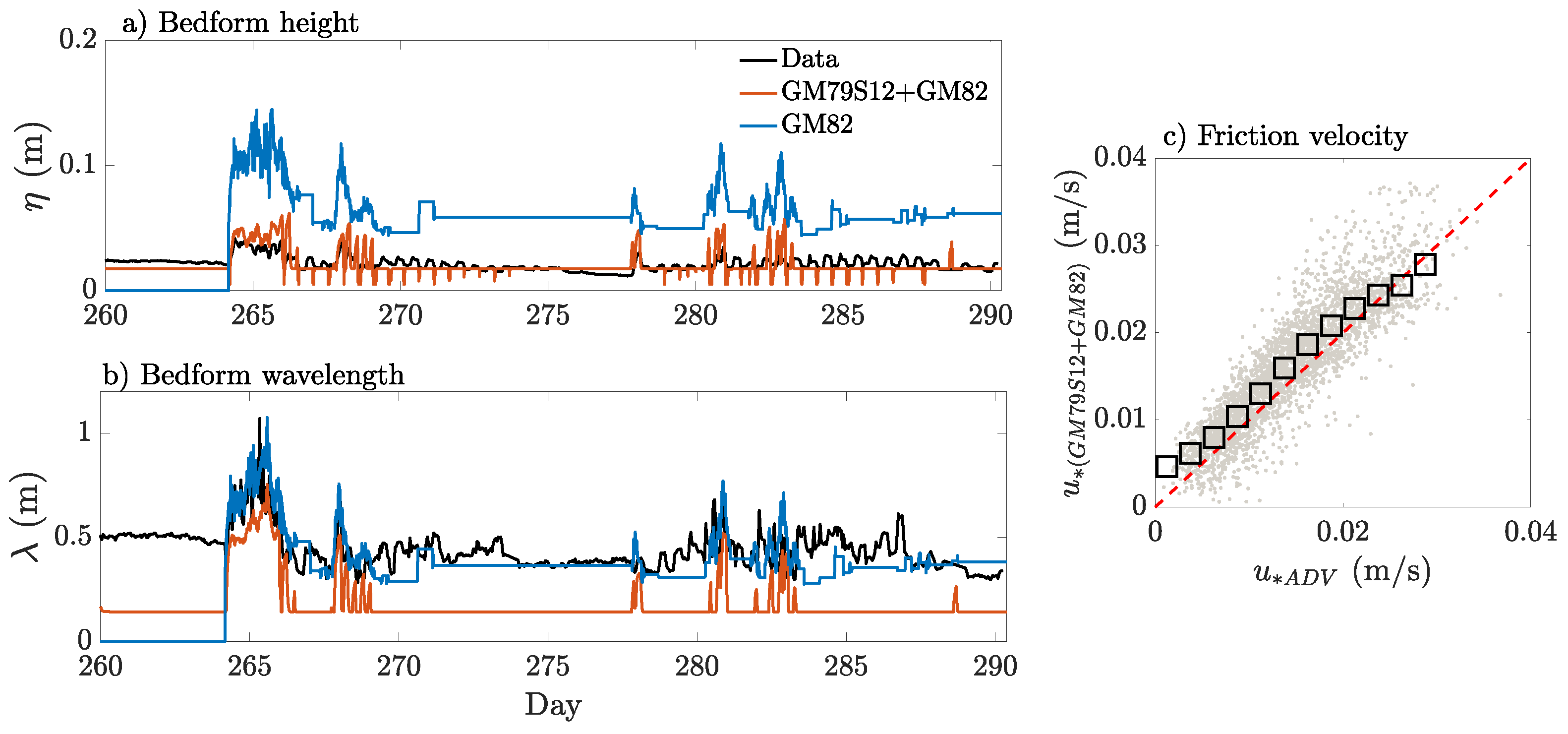
4.3.2. Bedform Predictors and Time-Evolving Ripple Dynamics
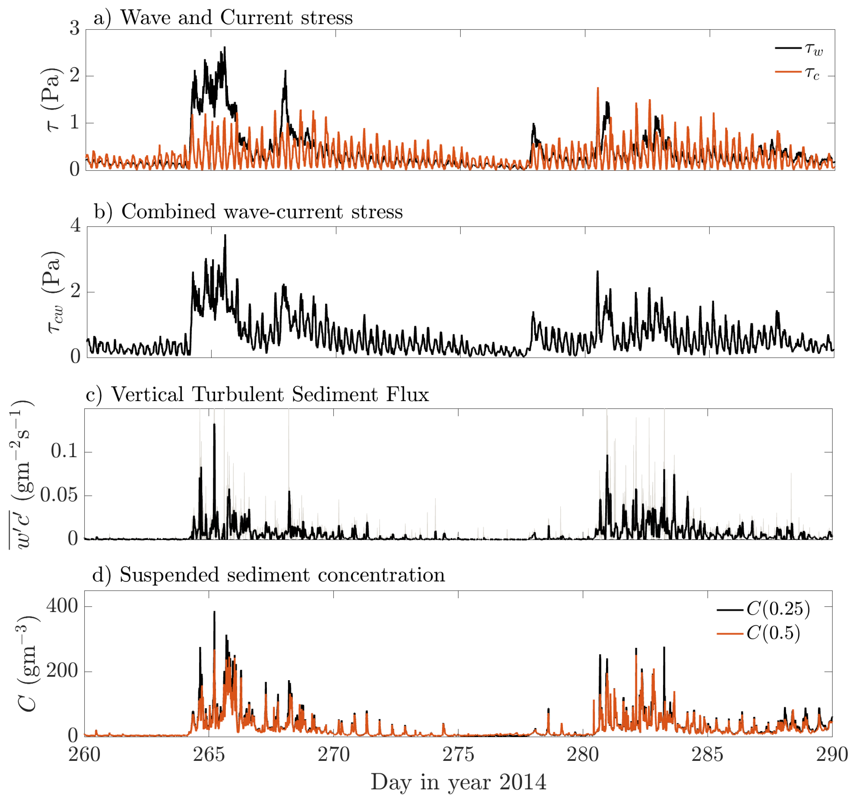
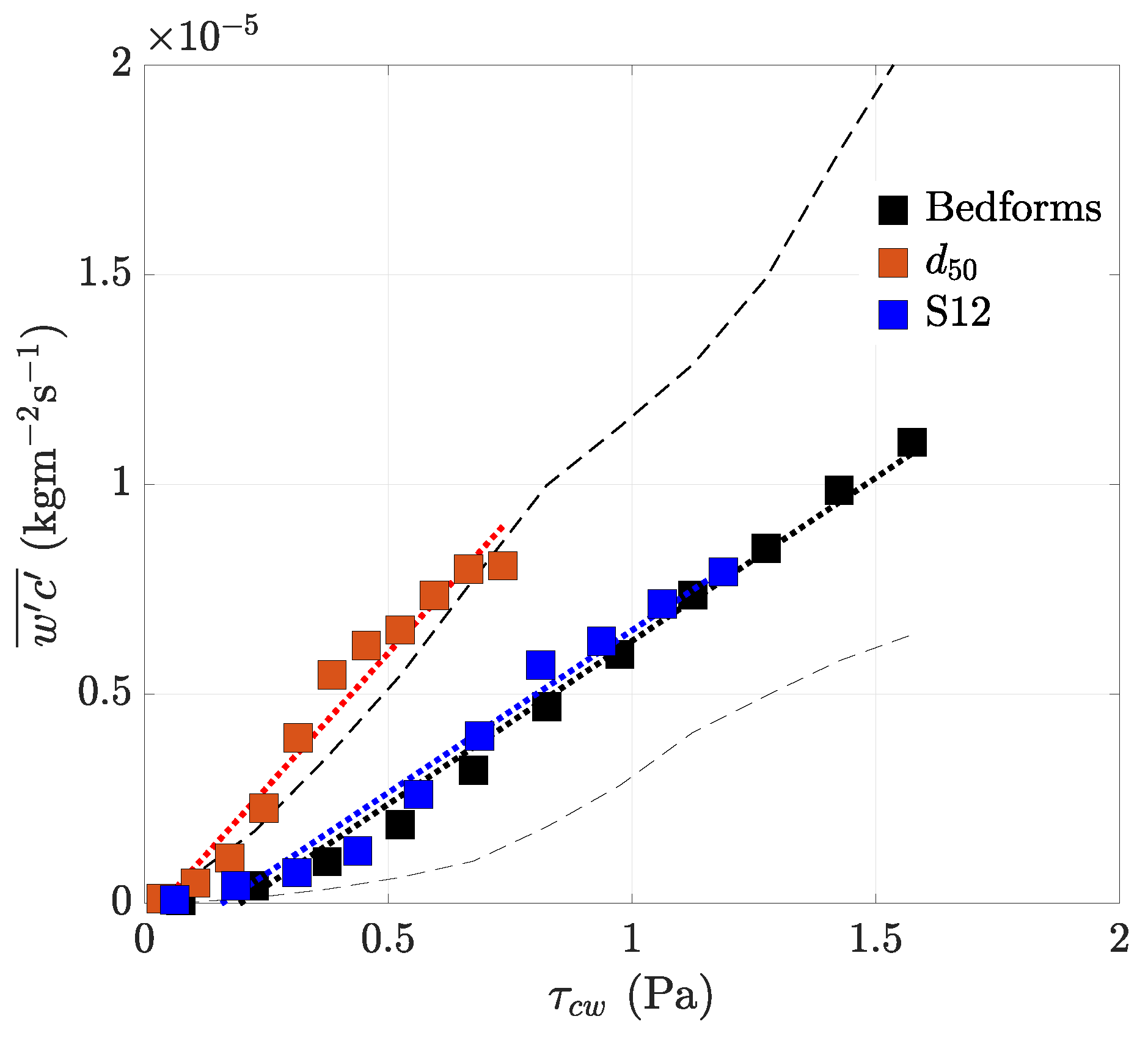
4.4. Turbulent Sediment Fluxes
5. Discussion
5.1. Non-Equilibrium Ripple Dynamics
5.2. Fine Sediment Resuspension
6. Summary and Conclusions
Author Contributions
Funding
Informed Consent Statement
Data Availability Statement
Acknowledgments
Conflicts of Interest
References
- Yoshiyama, K.; Sharp, J.H. Phytoplankton response to nutrient enrichment in an urbanized estuary: Apparent inhibition of primary production by overeutrophication. Limnol. Oceanogr. 2006, 51, 424–434. [Google Scholar] [CrossRef]
- Winterwerp, J.C.; Wang, Z.B.; van Braeckel, A.; van Holland, G.; Kösters, F. Man-induced regime shifts in small estuaries—II: A comparison of Rivers. Ocean. Dyn. 2013, 63, 1293–1306. [Google Scholar] [CrossRef]
- Admiraal, D.M.; García, M.H.; Rodriguez, J.F. Entrainment response of bed sediment to time-varying flows. Water Resour. Res. 2000, 36, 335–348. [Google Scholar] [CrossRef]
- Grant, W.D.; Madsen, O.S. Combined wave and current interaction with a rough bottom. J. Geophys. Res. Ocean. 1979, 84, 1797–1808. [Google Scholar] [CrossRef]
- Bolaños, R.; Thorne, P.D.; Wolf, J. Comparison of measurements and models of bed stress, bedforms and suspended sediments under combined currents and waves. Coast. Eng. 2012, 62, 19–30. [Google Scholar] [CrossRef]
- Scully, M.E.; Trowbridge, J.H.; Sherwood, C.R.; Jones, K.R.; Traykovski, P. Direct measurements of mean reynolds stress and ripple roughness in the presence of energetic forcing by surface waves. J. Geophys. Res. Ocean. 2018, 123, 2494–2512. [Google Scholar] [CrossRef]
- Soulsby, R.; Hamm, L.; Klopman, G.; Myrhaug, D.; Simons, R.; Thomas, G. Wave-current interaction within and outside the bottom boundary layer. Coast. Eng. 1993, 21, 41–69. [Google Scholar] [CrossRef]
- Wiberg, P.L.; Drake, D.E.; Cacchione, D.A. Sediment resuspension and bed armoring during high bottom stress events on the Northern California inner continental shelf: Measurements and predictions. Cont. Shelf Res. 1994, 14, 1191–1219. [Google Scholar] [CrossRef]
- Styles, R.; Glenn, S.M. Modeling stratified wave and current bottom boundary layers on the continental shelf. J. Geophys. Res. Ocean. 2000, 105, 24119–24139. [Google Scholar] [CrossRef]
- Lacy, J.R.; Sherwood, C.R.; Wilson, D.J.; Chisholm, T.A.; Gelfenbaum, G.R. Estimating hydrodynamic roughness in a wave-dominated environment with a high-resolution acoustic Doppler profiler. J. Geophys. Res. Ocean. 2005, 110, C06014. [Google Scholar] [CrossRef]
- Li, M.Z.; Amos, C.L. Predicting ripple geometry and bed roughness under combined waves and currents in a continental shelf environment. Cont. Shelf Res. 1998, 18, 941–970. [Google Scholar] [CrossRef]
- Traykovski, P.; Hay, A.E.; Irish, J.D.; Lynch, J.F. Geometry, migration, and evolution of wave orbital ripples at LEO-15. J. Geophys. Res. Ocean. 1999, 104, 1505–1524. [Google Scholar] [CrossRef]
- Soulsby, R.; Whitehouse, R.; Marten, K. Prediction of time-evolving sand ripples in shelf seas. Cont. Shelf Res. 2012, 38, 47–62. [Google Scholar] [CrossRef]
- Drake, D.E.; Cacchione, D.A. Wave—Current interaction in the bottom boundary layer during storm and non-storm conditions: Observations and model predictions. Cont. Shelf Res. 1992, 12, 1331–1352. [Google Scholar] [CrossRef]
- Drake, D.E.; Cacchione, D.A.; Grant, W.D. Shear stress and bed roughness estimates for combined wave and current flows over a rippled bed. J. Geophys. Res. Ocean. 1992, 97, 2319–2326. [Google Scholar] [CrossRef]
- Chalmoukis, I.A.; Dimas, A.A.; Grigoriadis, D.G. Large-eddy simulation of turbulent oscillatory flow over three-dimensional transient vortex ripple geometries in quasi-equilibrium. J. Geophys. Res. Earth Surf. 2020, 125, e2019JF005451. [Google Scholar] [CrossRef]
- Grant, W.D.; Madsen, O.S. Movable bed roughness in unsteady oscillatory flow. J. Geophys. Res. Ocean. 1982, 87, 469–481. [Google Scholar] [CrossRef]
- Nielsen, P. Dynamics and geometry of wave-generated ripples. J. Geophys. Res. Ocean. 1981, 86, 6467–6472. [Google Scholar] [CrossRef]
- Soulsby, R. Dynamics of Marine Sands: A Manual for Practical Applications; Thomas Telford: London, UK, 1997. [Google Scholar]
- Wiberg, P.L.; Harris, C.K. Ripple geometry in wave-dominated environments. J. Geophys. Res. Ocean. 1994, 99, 775–789. [Google Scholar] [CrossRef]
- Nelson, T.R.; Voulgaris, G.; Traykovski, P. Predicting wave-induced ripple equilibrium geometry. J. Geophys. Res. Ocean. 2013, 118, 3202–3220. [Google Scholar] [CrossRef]
- Faraci, C.; Foti, E.; Musumeci, R. Waves plus currents at a right angle: The rippled bed case. J. Geophys. Res. Ocean. 2008, 113, C07018. [Google Scholar] [CrossRef]
- Traykovski, P.; Wiberg, P.L.; Geyer, W.R. Observations and modeling of wave-supPorted sediment gravity flows on the Po prodelta and comparison to prior observations from the Eel shelf. Cont. Shelf Res. 2007, 27, 375–399. [Google Scholar] [CrossRef]
- Davis, J.P.; Walker, D.J.; Townsend, M.; Young, I.R. Wave-formed sediment ripples: Transient analysis of ripple spectral development. J. Geophys. Res. Ocean. 2004, 109, C07020. [Google Scholar] [CrossRef]
- Nelson, T.R.; Voulgaris, G. TemPoral and spatial evolution of wave-induced ripple geometry: Regular versus irregular ripples. J. Geophys. Res. Ocean. 2014, 119, 664–688. [Google Scholar] [CrossRef]
- O’Donoghue, T.; Clubb, G.S. Sand ripples generated by regular oscillatory flow. Coast. Eng. 2001, 44, 101–115. [Google Scholar] [CrossRef]
- Traykovski, P. Observations of wave orbital scale ripples and a nonequilibrium time-dependent model. J. Geophys. Res. Ocean. 2007, 112, C06026. [Google Scholar] [CrossRef]
- Nelson, T.R.; Voulgaris, G. A spectral model for estimating temPoral and spatial evolution of rippled seabeds. Ocean. Dyn. 2015, 65, 155–171. [Google Scholar] [CrossRef]
- Partheniades, E. Erosion and dePosition of cohesive soils. J. Hydraul. Div. 1965, 91, 105–139. [Google Scholar] [CrossRef]
- Van Prooijen, B.; Winterwerp, J. A stochastic formulation for erosion of cohesive sediments. J. Geophys. Res. Ocean. 2010, 115, C01005. [Google Scholar] [CrossRef]
- Madsen, O.S. Spectral wave-current bottom boundary layer flows. In Coastal Engineering 1994; ASCE: Reston, VA, USA, 1995; pp. 384–398. [Google Scholar]
- Malarkey, J.; Davies, A.G. A non-iterative procedure for the Wiberg and Harris (1994) oscillatory sand ripple predictor. J. Coast. Res. 2003, 19, 738–739. [Google Scholar]
- Pedocchi, F.; Garcia, M. Ripple morphology under oscillatory flow: 1. Prediction. J. Geophys. Res. Ocean. 2009, 114, C12014. [Google Scholar] [CrossRef]
- Baas, J.H. Dimensional Analysis of Current Ripples in Recent and Ancient dePositional Environments; Faculty of Geosciences, Utrecht University: Utrecht, The Netherlands, 1993. [Google Scholar]
- Soulsby, R.; Whitehouse, R. Threshold of sediment motion in coastal environments. In Proceedings of the Pacific Coasts and Ports’ 97: Proceedings of the 13th Australasian Coastal and Ocean Engineering Conference and the 6th Australasian Port and Harbour Conference; Centre for Advanced Engineering, University of Canterbury: Christchurch, New Zealand, 1997; Volume 1, p. 145. [Google Scholar]
- Horner-Devine, A.R.; Pietrzak, J.D.; Souza, A.J.; McKeon, M.A.; Meirelles, S.; Henriquez, M.; Flores, R.P.; Rijnsburger, S. Cross-shore transPort of nearshore sediment by River plume frontal pumping. Geophys. Res. Lett. 2017, 44, 6343–6351. [Google Scholar] [CrossRef]
- Flores, R.P.; Rijnsburger, S.; Horner-Devine, A.R.; Souza, A.J.; Pietrzak, J.D. The impact of storms and stratification on sediment transPort in the Rhine region of freshwater influence. J. Geophys. Res. Ocean. 2017, 122, 4456–4477. [Google Scholar] [CrossRef]
- Rijnsburger, S.; Flores, R.P.; Pietrzak, J.D.; Horner-Devine, A.R.; Souza, A.J. The influence of tide and wind on the propagation of fronts in a shallow River plume. J. Geophys. Res. Ocean. 2018, 123, 5426–5442. [Google Scholar] [CrossRef]
- Stive, M.J.; de Schipper, M.A.; Luijendijk, A.P.; Aarninkhof, S.G.; van Gelder-Maas, C.; van Thiel de Vries, J.S.; de Vries, S.; Henriquez, M.; Marx, S.; Ranasinghe, R. A new alternative to saving our beaches from sea-level rise: The Sand Engine. J. Coast. Res. 2013, 29, 1001–1008. [Google Scholar] [CrossRef]
- Huisman, B.; De Schipper, M.; Ruessink, B. Sediment sorting at the Sand Motor at storm and annual time scales. Mar. Geol. 2016, 381, 209–226. [Google Scholar] [CrossRef]
- Meirelles, S.; Henriquez, M.; Souza, A.J.; Horner-Devine, A.R.; Pietrzak, J.D.; Rijnsburg, S.; Stive, M.J. Small Scale Bedform Types off the South-Holland Coast. J. Coast. Res. 2016, 75, 423–426. [Google Scholar] [CrossRef]
- Perron, J.T.; Kirchner, J.W.; Dietrich, W.E. Spectral signatures of characteristic spatial scales and nonfractal structure in landscapes. J. Geophys. Res. Earth Surf. 2008, 113, F04003. [Google Scholar] [CrossRef]
- Flores, R.P.; Rijnsburger, S.; Meirelles, S.; Horner-Devine, A.R.; Souza, A.J.; Pietrzak, J.D.; Henriquez, M.; Reniers, A. Wave generation of gravity-driven sediment flows on a predominantly sandy seabed. Geophys. Res. Lett. 2018, 45, 7634–7645. [Google Scholar] [CrossRef]
- Goring, D.G.; Nikora, V.I. Despiking acoustic Doppler velocimeter data. J. Hydraul. Eng. 2002, 128, 117–126. [Google Scholar] [CrossRef]
- Shaw, W.J.; Trowbridge, J.H. The direct estimation of near-bottom turbulent fluxes in the presence of energetic wave motions. J. Atmos. Ocean. Technol. 2001, 18, 1540–1557. [Google Scholar] [CrossRef]
- Kim, S.C.; Friedrichs, C.; Maa, J.Y.; Wright, L. Estimating bottom stress in tidal boundary layer from acoustic Doppler velocimeter data. J. Hydraul. Eng. 2000, 126, 399–406. [Google Scholar] [CrossRef]
- Brand, A.; Lacy, J.R.; Hsu, K.; Hoover, D.; Gladding, S.; Stacey, M.T. Wind-enhanced resuspension in the shallow waters of South San Francisco Bay: Mechanisms and Potential implications for cohesive sediment transPort. J. Geophys. Res. Ocean. 2010, 115, C11024. [Google Scholar] [CrossRef]
- Brand, A.; Lacy, J.R.; Gladding, S.; Holleman, R.; Stacey, M. Model-based interpretation of sediment concentration and vertical flux measurements in a shallow estuarine environment. Limnol. Oceanogr. 2015, 60, 463–481. [Google Scholar] [CrossRef]
- Voulgaris, G.; Meyers, S.T. TemPoral variability of hydrodynamics, sediment concentration and sediment settling velocity in a tidal creek. Cont. Shelf Res. 2004, 24, 1659–1683. [Google Scholar] [CrossRef]
- Fugate, D.C.; Friedrichs, C.T. Determining concentration and fall velocity of estuarine particle Populations using ADV, OBS and LISST. Cont. Shelf Res. 2002, 22, 1867–1886. [Google Scholar] [CrossRef]
- Lynch, J.; Gross, T.; Sherwood, C.; Irish, J.; Brumley, B. Acoustical and optical backscatter measurements of sediment transPort in the 1988–1989 STRESS experiment. Cont. Shelf Res. 1997, 17, 337–366. [Google Scholar] [CrossRef]
- Wiberg, P.L.; Sherwood, C.R. Calculating wave-generated bottom orbital velocities from surface-wave parameters. Comput. Geosci. 2008, 34, 1243–1262. [Google Scholar] [CrossRef]
- Simpson, J.; Souza, A. Semidiurnal switching of stratification in the region of freshwater influence of the Rhine. J. Geophys. Res. Ocean. 1995, 100, 7037–7044. [Google Scholar] [CrossRef]
- De Boer, G.J.; Pietrzak, J.D.; Winterwerp, J.C. On the vertical structure of the Rhine region of freshwater influence. Ocean. Dyn. 2006, 56, 198–216. [Google Scholar] [CrossRef]
- Flores, R.P.; Rijnsburger, S.; Horner-Devine, A.R.; Kumar, N.; Souza, A.J.; Pietrzak, J.D. The formation of turbidity maximum zones by minor axis tidal straining in regions of freshwater influence. J. Phys. Oceanogr. 2020, 50, 1265–1287. [Google Scholar] [CrossRef]
- Nielsen, P. Coastal Bottom Boundary Layers and Sediment Transport; World Scientific Publishing Company: Singapore, 1992; Volume 4. [Google Scholar]
- Marsh, S.; Vincent, C.; Osborne, P. Bedforms in a laboratory wave flume: An evaluation of predictive models for bedform wavelengths. J. Coast. Res. 1999, 15, 624–634. [Google Scholar]
- Sanford, L.P.; Maa, J.P.Y. A unified erosion formulation for fine sediments. Mar. Geol. 2001, 179, 9–23. [Google Scholar] [CrossRef]
- Grabowski, R.C.; DropPo, I.G.; Wharton, G. Erodibility of cohesive sediment: The imPortance of sediment properties. Earth-Sci. Rev. 2011, 105, 101–120. [Google Scholar] [CrossRef]
- Sherwood, C.R.; Aretxabaleta, A.L.; Harris, C.K.; Rinehimer, J.P.; Verney, R.; Ferré, B. Cohesive and mixed sediment in the regional ocean modeling system (ROMS v3. 6) implemented in the Coupled Ocean–Atmosphere–Wave–Sediment Transport Modeling System (COAWST r1234). Geosci. Model Dev. 2018, 11, 1849–1871. [Google Scholar] [CrossRef]
- Van Kessel, T.; Winterwerp, H.; Van Prooijen, B.; Van Ledden, M.; Borst, W. Modelling the seasonal dynamics of SPM with a simple algorithm for the buffering of fines in a sandy seabed. Cont. Shelf Res. 2011, 31, S124–S134. [Google Scholar] [CrossRef]
- Dickhudt, P.J.; Friedrichs, C.T.; Sanford, L.P. Mud matrix solids fraction and bed erodibility in the York River estuary, USA, and other muddy environments. Cont. Shelf Res. 2011, 31, S3–S13. [Google Scholar] [CrossRef]


| Case | M (kg/m−2s−1Pa−1) | (Pa) |
|---|---|---|
| Bedforms | 7.78 × | 0.19 |
| d50 | 1.28 × | 0.03 |
| S12 | 7.74 × | 0.15 |
| GM82 | 2.94 × | 0.3 |
| WH94 | 3.27 × | 0.32 |
| PG09 | 4.08 × | 0.13 |
Disclaimer/Publisher’s Note: The statements, opinions and data contained in all publications are solely those of the individual author(s) and contributor(s) and not of MDPI and/or the editor(s). MDPI and/or the editor(s) disclaim responsibility for any injury to people or property resulting from any ideas, methods, instructions or products referred to in the content. |
© 2024 by the authors. Licensee MDPI, Basel, Switzerland. This article is an open access article distributed under the terms and conditions of the Creative Commons Attribution (CC BY) license (https://creativecommons.org/licenses/by/4.0/).
Share and Cite
Flores, R.P.; Rijnsburger, S.; Meirelles, S.; Horner-Devine, A.R.; Souza, A.J.; Pietrzak, J.D. Incorporating Non-Equlibrium Ripple Dynamics into Bed Stress Estimates Under Combined Wave and Current Forcing. J. Mar. Sci. Eng. 2024, 12, 2116. https://doi.org/10.3390/jmse12122116
Flores RP, Rijnsburger S, Meirelles S, Horner-Devine AR, Souza AJ, Pietrzak JD. Incorporating Non-Equlibrium Ripple Dynamics into Bed Stress Estimates Under Combined Wave and Current Forcing. Journal of Marine Science and Engineering. 2024; 12(12):2116. https://doi.org/10.3390/jmse12122116
Chicago/Turabian StyleFlores, Raúl P., Sabine Rijnsburger, Saulo Meirelles, Alexander R. Horner-Devine, Alejandro J. Souza, and Julie D. Pietrzak. 2024. "Incorporating Non-Equlibrium Ripple Dynamics into Bed Stress Estimates Under Combined Wave and Current Forcing" Journal of Marine Science and Engineering 12, no. 12: 2116. https://doi.org/10.3390/jmse12122116
APA StyleFlores, R. P., Rijnsburger, S., Meirelles, S., Horner-Devine, A. R., Souza, A. J., & Pietrzak, J. D. (2024). Incorporating Non-Equlibrium Ripple Dynamics into Bed Stress Estimates Under Combined Wave and Current Forcing. Journal of Marine Science and Engineering, 12(12), 2116. https://doi.org/10.3390/jmse12122116