Sensitivity Analysis of Underwater Structural-Acoustic Problems Based on Coupled Finite Element Method/Fast Multipole Boundary Element Method with Non-Uniform Rational B-Splines

Abstract

For the direct differentiation technique-based modeling of acoustic fluid–structure interaction and structural-acoustic sensitivity analysis, a coupling algorithm based on the finite element method (FEM) and the fast multipole boundary element method (FMBEM) is suggested. By bypassing the challenging volume parameterization process in isogeometric finite element techniques and the laborious meshing process in traditional FEM/BEM, non-uniform rational B-splines (NURBS) isogeometric analysis (IGA) is utilized to immediately perform numerical analysis on CAD models. The matrix-vector products in the boundary element analysis are accelerated using the fast multipole method (FMM). To hasten the solution of the linear system of equations, the iterative solver GMRES is used. The numerical prediction of the effects of arbitrarily shaped vibrating structures on the sound field is made feasible by the FEM/FMBEM technique. A number of numerical examples are provided to show the applicability and effectiveness of the suggested approach.

1. Introduction

Underwater acoustics frequently deal with the analysis of acoustic radiation or scattering from elastic objects in heavy fluid. It is only possible to find analytical solutions for acoustic fluid–structure interaction [1] issues when the structure has simple geometry and simple boundary conditions. More real-world problems with complicated geometries cannot be solved analytically; thus, efficient numerical approaches must be devised.

The dynamic behavior of problems involving fluid–structure interactions, acoustics, fracture mechanics, and electromagnetics has been widely studied using FEM. However, there are a number of problems with the FEM when modeling infinite domains. As is commonly known, the BEM has been effectively used to address acoustic concerns as it offers superior precision and straightforward mesh formation. Particularly for exterior acoustic problems, the Sommerfeld radiation condition at infinity is immediately satisfied [2]. The boundary integral problem has been quantitatively solved using the Galerkin approach for BEM implementation [3,4]. However, the engineering community has always favored the collocation technique. Therefore, the examination of problems with fluid–structure interaction is acceptable for the coupled FEM/BEM approach [5,6]. However, due to the CBEM’s generation of a dense and non-symmetric coefficient matrix that requires O(N${}^3$) arithmetic operations to directly resolve the equation system, for example, when employing the Gauss elimination approach, coupling analysis of underwater structural-acoustic problems continues to be the bottleneck of high computational cost. The fast multipole method (FMM), the fast direct solver, and the adaptive cross approximation approach are just a few of the methods that have been utilized to expedite the resolution of the integral issue. The rapid direct solver was developed by Martinsson and Rokhlin [7,8]. It quickly creates a reduced factorization of the matrix’s inverse and performs well for problems requiring moderately ill-conditioned matrices. For problems needing a lot of iterations, the Bebendorf and Rjasanow-invented adaptive cross approximation approach [9] creates blockwise low-rank approximants from the BEM matrices. The CBEM system of equations may now be solved more quickly thanks to the development of FMM [10,11,12,13,14]. Therefore, utilizing a coupling strategy based on FEM/fast multipole boundary element method (FEM/FMBEM) [15], it may be possible to handle large-scale fluid–structure interaction problems. This study also recommends the coupling method FEM/FMBEM to handle the challenging problems involving fluid–structure interactions.

Design professionals are increasingly taking into account passive noise management by changing the geometry of constructions. This structural-acoustic optimization has great potential for reducing radiated noise [16,17], especially for thin-shell constructions. Because it may demonstrate how a geometry adjustment impacts the structure’s acoustic performance, acoustic design sensitivity analysis is an essential stage in the procedures of acoustic design and optimization. The advancement of passive noise elimination through structural-acoustic optimization is summarized by Marburg [18]. The finite difference method (FDM) has been utilized extensively for structural-acoustic optimization [19,20,21] because of how easy it is to apply. Yet, this approach has poor performance, especially when numerous design factors are given consideration at once. To solve this problem, we use the adjoint variable method (AVM) [22,23] or the direct differentiation method (DDM) [24]. The sensitivity analysis for the fluid–structure interaction problem, as is well known, takes up the greatest time in the gradient-based optimization procedure. In order to speed up the analysis, the coupling method FEM/FMBEM is subjected to the structural-acoustic sensitivity analysis based on DDM in this work.

The FEM and BEM may be applied with the help of suitable software; this technique is called computer-aided engineering (CAE). Modern CAE requires, however, that the models produced by CAD software be converted into simulation-ready models as part of the preprocessing step. Geometric model data transfer in the CAE results in geometry errors. A proposed solution to this problem is the integration of boundary element method (IGABEM) [25,26] with geometric modeling and numerical simulation utilizing isogeometric analysis [27,28,29]. Geometric errors and laborious preprocessing processes may be eliminated, and numerical simulation can be performed directly from the accurate models, all thanks to IGABEM. Elastic mechanics [30], potential difficulties [31,32], wave propagation [33,34], fracture mechanics [35], electromagnetics [36,37,38], and structural optimization [39,40,41,42,43,44] are just a few of the problems that IGABEM has been utilized to solve since its founding. The NURBS IGABEM is used in this investigation.

This work develops the sensitivity formulation for the coupled FEM/BEM analysis and adds FMBEM to the structural-acoustic coupling sensitivity analysis. Coupling FEM/FMBEM is recommended for issues involving fluid–structure interaction and structural acoustic sensitivity assessments. NURBS is applied for the first time to structural-acoustic coupling calculations and acoustic sensitivity analysis, which eliminates geometric errors and improves the calculation accuracy. The precision and effectiveness of this method are demonstrated using numerical examples.

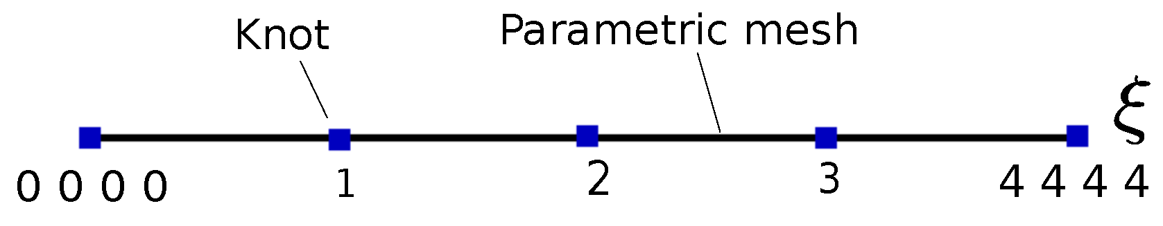
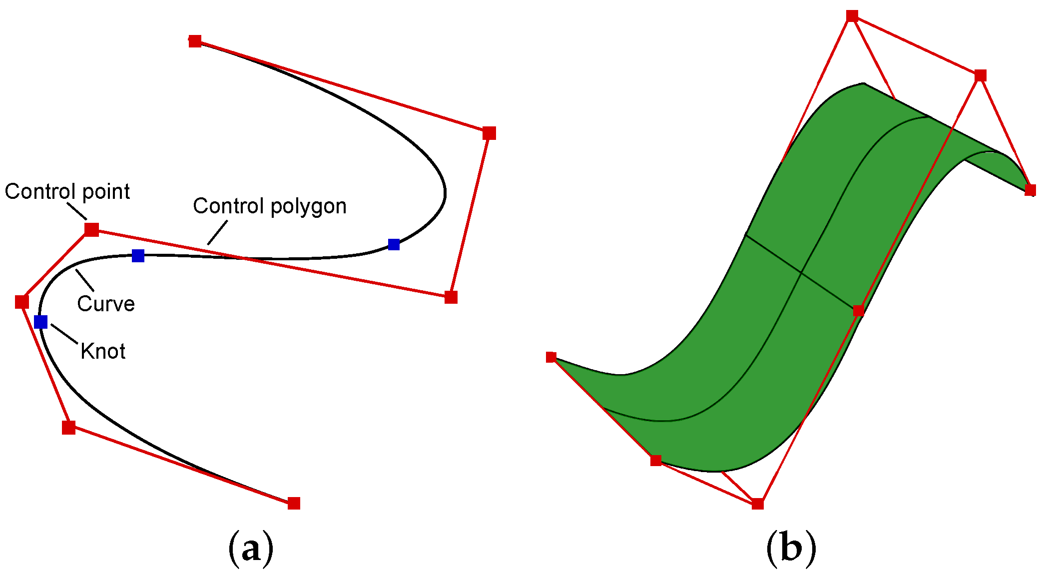
2. Non-Uniform Rational B-Splines (NURBS)

In order to be thorough, this part addresses some of the fundamental NURBS ideas that are the basis of the isogeometric analysis. The readers are directed to [27,45] for further information. The knot vector made up by a collection of non-decreasing real numbers represented as in Equation (1) is a key idea in NURBS.

$$\Xi =\left[{\xi }_1,{\xi }_2,\cdots ,{\xi }_{n+p+1}\right],{\xi }_a\in \mathbb{R},$$

(1)

where n is the overall amount of basis functions, p is the polynomial order, and a is the knot index. One may think of a knot vector as a parametric space in one dimension, as shown in Figure 1.

The Cox-de Boor recursion formula is used to express the B-spline basis functions for a given knot vector, as presented in Equations (2) and (3). When $p=0$, we have

$$N_{a,0}\left(\xi \right)=\left\{\begin{array}{c}1\mathrm{if}{\xi }_a\le \xi <{\xi }_{a+1},\hfill \\ 0\mathrm{otherwise},\hfill \end{array}\right.$$

(2)

and when $p\ge 1$,

$$\begin{array}{c}\hfill N_{a,p}\left(\xi \right)={\displaystyle \frac{\xi -{\xi }_a}{{\xi }_{a+p}-{\xi }_a}}{N}_{a,p-1}\left(\xi \right)+{\displaystyle \frac{{\xi }_{a+p+1}-\xi }{{\xi }_{a+p+1}-{\xi }_{a+1}}}{N}_{a+1,p-1}\left(\xi \right).\end{array}$$

(3)

Numerous advantageous characteristics of B-spline basis functions (as demonstrated in Figure 2, different colors representing different orders of NURBS basis functions), including linear independence and local support, make them suitable for numerical analysis. As demonstrated in Equation (4), the B-spline curve may be created by linearly combining B-spline basis functions and control points.

$${\displaystyle \mathbf{x}\left(\xi \right)=\sum _{i=1}^n{N}_{a,p}\left(\xi \right){\mathbf{P}}_{a,p},}$$

(4)

where the control point coordinates are represented by the coefficients P${}_{a,b}$. Because of this, a B-spline curve is fundamentally a conversion from a parametric one-dimensional space to actual space. There are the following knot vectors in every dimension of the following two-dimensional parametric spaces:

$$\begin{array}{c}\hfill \left[{\xi }_1,{\xi }_2,\cdots ,{\xi }_{n+p+1}\right],{\xi }_a\in \mathbb{R},\end{array}$$

(5)

$$\begin{array}{c}\hfill \left[{\eta }_1,{\eta }_2,\cdots ,{\eta }_{m+l+1}\right],{\xi }_b\in \mathbb{R}.\end{array}$$

(6)

The tensor product property may be used to build the B-spline surface, as illustrated in Equation (7).

$${\displaystyle \mathbf{x}(\xi ,\eta )=\sum _{a=1}^n\sum _{b=1}^m{N}_{a,p}\left(\xi \right)N_{b,l}\left(\eta \right){\mathbf{P}}_{a,b},}$$

(7)

where n and m are the corresponding numbers of basis functions in each dimension. It should be mentioned that B-spline control points are not usually on the surface (as demonstrated in Figure 3) due to the absence of the Kronecker delta property (as demonstrated in Figure 2).

By linking a weight coefficient with every control point, NURBS extend B-splines. Using NURBS, designers may precisely represent various curves having conic segments, like ellipses and circles, and gain more control over the depicted curve without boosting the degree or the quantity of control points. The NURBS basis functions are constructed from the B-spline basis functions, which are represented in two dimensions as Equation (8).

$$\begin{array}{cc}\hfill R_{a,b}(\xi ,\eta )& ={\displaystyle \frac{N_{b,p}\left(\xi \right)N_{b,l}\left(\eta \right)w_{a,b}}{W(\xi ,\eta )}},\hfill \\ \hfill W(\xi ,\eta )& {\displaystyle =\sum _{a=1}^n\sum _{b=1}^m{N}_{a,p}\left(\xi \right)N_{b,l}\left(\eta \right)w_{a,b}.}\hfill \end{array}$$

(8)

where w is the weight coefficient. Similar to how B-spline surfaces are formed, NURBS basis functions and control points are used to define NURBS surfaces, as indicated in Equation (9).

$${\displaystyle \mathbf{x}(\xi ,\eta )=\sum _{a=1}^n\sum _{b=1}^m{R}_{a,p}\left(\xi \right)R_{b,l}\left(\eta \right){\mathbf{P}}_{a,b}.}$$

(9)

Equation (9) may be recast as Equation (10) by dropping the notation p in the following and iterating between basis functions or control points using the global index A.

$$\begin{array}{c}\hfill {\displaystyle \mathbf{x}(\xi ,\eta )=\sum _{A=1}^{N_A}{R}_A(\xi ,\eta ){\mathbf{P}}_A.}\end{array}$$

(10)

More control points can be added using the knot insertion operator without altering the structural form. By adopting the h-refinement method, this characteristic helps to increase the precision of estimating physical fields while maintaining geometric correctness.

3. Structural-Acoustic Coupling

3.1. FEM Analysis

Fritze et al. [6,46] detailed the whole structural-acoustic analysis technique, and associated expressions are provided in this section. If a harmonic load is given to the structure, it is possible to infer from the frequency response analysis what the structure’s steady-state reaction will be. The structural-acoustic equation’s linear system is derived in Equation (11).

$$\begin{array}{cc}\hfill \left(\mathbf{K}+\mathrm{i}\omega \mathbf{C}-{\omega }^2\mathbf{M}\right)\mathbf{u}\left(\omega \right)& =\mathbf{A}\mathbf{u},\hfill \end{array}$$

(11)

$$\begin{array}{cc}\hfill \mathbf{f}& =\mathbf{A}\mathbf{u},\hfill \end{array}$$

(12)

where K is the stiffness matrix, $\mathrm{i}=\sqrt{-1}$ the imaginary unit, $\omega$ the harmonic load’s excitation frequency, $\mathbf{C}$ the damping matrix, $\mathbf{M}$ the mass matrix, $\mathbf{u}$ the nodal displacement vector, and $\mathbf{f}$ the full excitation.

Note that, although the steady-state response maintains the same frequency with the applied load, damping may cause it to have a distinct phase angle. By breaking down the time-dependent impulses into the frequency domain, Equation (11) can still be applied in the event that the load being imposed is not harmonic. A coupling matrix is added to shift the structural nodal load from the fluid effect to fluid nodal pressure to consider how the acoustic pressure exerted on structural surfaces affects aspects. The full excitation, which combines the acoustic load and the structural load, might then be expressed using Equation (13).

$$\begin{array}{cc}\hfill \mathbf{f}& ={\mathbf{C}}_{\mathbf{sf}}\mathbf{p}+{\mathbf{f}}_{\mathbf{s}},\hfill \end{array}$$

(13)

$$\begin{array}{cc}\hfill {\mathbf{C}}_{\mathbf{sf}}& ={\int }_{{\Gamma }_{int}}{\mathbf{N}}_{\mathbf{s}}^{\mathbf{T}}\mathbf{n}{\mathbf{N}}_{\mathbf{f}}\mathrm{d}\Gamma ,\hfill \end{array}$$

(14)

where ${\mathbf{C}}_{\mathbf{sf}}$ is the coupling matrix, $\mathbf{p}$ the fluid nodal pressure, ${\mathbf{C}}_{\mathbf{sf}}\mathbf{p}$ the acoustic load denoting the effect of the acoustic pressure applied to the structural surfaces, ${\mathbf{f}}_{\mathbf{s}}$ the structural load, ${\mathbf{N}}_{\mathbf{s}}$ the interpolation function for structural domain, $\mathbf{n}$ the external normal direction of the structural surface, ${\mathbf{N}}_{\mathbf{f}}$ the interpolation function for the fluid domain, and $\Gamma$ the interaction surface situated between the areas of fluidity and structure.

The coupling matrix ${\mathbf{C}}_{\mathbf{sf}}$ directs the structural nodal load from the fluid effect to the fluid nodal pressure. Equation (15) may then be used to calculate the nodal displacement.

$$\mathbf{u}={\mathbf{A}}^{-1}\mathbf{f}.$$

(15)

The fluid loads applied on underwater bodies are very important. Rehman et al. [47] looked at a fast and less expensive semi-empirical method to determine the hydrodynamic coefficients for a convoluted transportation system with two UUVs. As for the details of the acoustic pressure applied to the structural surfaces mentioned above, please refer to Rehman et al. [47].

3.2. BEM Analysis

The time-harmonic wave field of sound in the Helmholtz equation is described by Equation (16), while the boundary conditions are expressed by Equation (17).

$${\nabla }^{2}p\left(x\right)+k^{2}p\left(x\right)=0,$$

(16)

$$\begin{array}{cc}\hfill p\left(x\right)& =\overline{p}\left(x\right)x\in {\Gamma }_p,\hfill \\ \hfill q\left(x\right)& =\frac{\partial p\left(x\right)}{\partial n\left(x\right)}=\mathrm{i}\rho \omega \overline{v}\left(x\right)x\in {\Gamma }_q,\hfill \\ \hfill p\left(x\right)& =zv\left(x\right)x\in {\Gamma }_z,\hfill \end{array}$$

(17)

where p is the sound pressure, k the wave number, $\overline{\left(\right)}$ the known function given on the border, ${\Gamma }_p$ the Dirichlet boundary condition, $\rho$ the structural density, $\omega$ the frequency of the incoming force, v the normal velocity, ${\Gamma }_q$ the Neumann boundary condition, z the acoustic impedance, and ${\Gamma }_z$ the Robin boundary condition.

From Equations (16) to (18), one may construct a boundary integral equation that is specific to the structural boundary $\Gamma$.

$$c\left(x\right)p\left(x\right)+{\int }_{\Gamma }F(x,y)p\left(y\right)\mathrm{d}\Gamma \left(y\right)={\int }_{\Gamma }G(x,y)q\left(y\right)\mathrm{d}\Gamma \left(y\right),$$

(18)

where x is the source point, y the field point, $c\left(x\right)$ = 1/2 if the boundary $\Gamma$ is smooth in the vicinity of the source point x, p the intensity of the incoming wave, $G(x,y)$ the Green’s function, q the normal derivative of p, and F the normal derivative of G.

For acoustic issues in three-dimensional problems, Equation (19) offers the expression of Green’s function $G(x,y)$.

$$\begin{array}{cc}\hfill G(x,y)& =\frac{e^{ikr}}{4\pi r},\hfill \end{array}$$

(19)

$$\begin{array}{cc}\hfill r& =\left|y-x\right|.\hfill \end{array}$$

(20)

In cases when the source point x has a smooth border $\Gamma$, the integral representation’s derivative in Equation (18) with reference to the outer normal at point x may be expressed as Equation (21).

$$\frac{1}{2}q\left(x\right)+{\int }_{\Gamma }\frac{\partial F(x,y)}{\partial n\left(x\right)}p\left(y\right)\mathrm{d}\Gamma \left(y\right)={\int }_{\Gamma }\frac{\partial G(x,y)}{\partial n\left(x\right)}q\left(y\right)\mathrm{d}\Gamma \left(y\right).$$

(21)

It is well known that nonuniqueness makes it difficult to apply a single Helmholtz boundary integral equation to problems requiring external boundary values. In this work, the method known as the Burton–Miller strategy [48] combining the linear Equations (18) and (21), is employed to successfully address the issue of nonuniqueness. The Hadamard finite part integral method and the Cauchy principal value may also be used to directly and efficiently compute the singular boundary integrals [24] brought about by Equations (18) and (21).

The system of linear algebraic equations shown in Equation (22) can be obtained [49] if the border $\Gamma$ is divided into elements by putting all of the collocation point equations for each element’s center together and presenting them using matrix representations.

$$\mathbf{H}\mathbf{p}=\mathbf{G}\mathbf{q}+{\mathbf{p}}_{\mathbf{i}},$$

(22)

where ${\mathbf{p}}_{\mathbf{i}}$ is the nodal pressure brought on by the incoming wave.

3.3. FEM–BEM Coupling Analysis

The precise FEM/BEM modeling formulas were published by Fritze et al. [6], and associated expressions are provided in this section. The governing equations, as described in the preceding section, are connected by the continuity constraint across the interaction surface, as indicated in Equation (23). Then, in accordance with Equation (24), it is reasonable to represent the normal velocity $\mathbf{v}$ as a function of the displacement $\mathbf{u}$.

$$\begin{array}{cc}\hfill \mathbf{q}& =-\mathrm{i}\omega \rho \mathbf{v},\hfill \end{array}$$

(23)

$$\begin{array}{cc}\hfill \mathbf{v}& =\mathrm{i}\omega {\mathbf{S}}^{-\mathbf{1}}{\mathbf{C}}_{\mathbf{fs}}\mathbf{u},\hfill \end{array}$$

(24)

$$\begin{array}{cc}\hfill \mathbf{S}& ={\int }_{{\Gamma }_{int}}{\mathbf{N}}_{\mathbf{f}}^{\mathbf{T}}{\mathbf{N}}_{\mathbf{f}}\mathrm{d}\Gamma ,\hfill \end{array}$$

(25)

$$\begin{array}{cc}\hfill {\mathbf{C}}_{\mathbf{fs}}& ={\mathbf{C}}_{\mathbf{sf}}^{\mathbf{T}}.\hfill \end{array}$$

(26)

By adding Equations (24) to (22), we may obtain Equation (27). As shown in Equation (28), Equations (11) and (27) can be joined to create an equation system.

$$\mathbf{H}\mathbf{p}={\omega }^2\rho {\mathbf{GS}}^{-\mathbf{1}}{\mathbf{C}}_{\mathbf{fs}}\mathbf{u}+{\mathbf{p}}_{\mathbf{i}}.$$

(27)

$$\left[\begin{array}{cc}\mathbf{A}& -{\mathbf{C}}_{\mathbf{sf}}\\ -{\omega }^2\rho \mathbf{G}{\mathbf{S}}^{-\mathbf{1}}{\mathbf{C}}_{\mathbf{fs}}& \mathbf{H}\end{array}\right]\left\{\begin{array}{c}\mathbf{u}\\ \mathbf{p}\end{array}\right\}=\left\{\begin{array}{c}{\mathbf{f}}_{\mathbf{s}}\\ {\mathbf{p}}_{\mathbf{i}}\end{array}\right\}.$$

(28)

As a result of the sluggish convergence of the direct iterations on Equation (28), the direct system equation solution would require significantly greater processing power and storage capacity. It is also difficult to obtain highly precise numerical results. We deliver the subsequent method to solve the above non-symmetric linear system without utilizing an iterative solution. You may obtain the coupled boundary element equation [6] in Equation (29) by substituting Equation (15) into Equation (27).

$$\begin{array}{cc}\hfill \mathbf{Hp}-{\mathbf{GWC}}_{\mathbf{sf}}\mathbf{p}& ={\mathbf{GWf}}_{\mathbf{s}}+{\mathbf{p}}_{\mathbf{i}},\hfill \end{array}$$

(29)

$$\begin{array}{cc}\hfill \mathbf{W}& ={\omega }^2\rho {\mathbf{S}}^{-\mathbf{1}}{\mathbf{C}}_{\mathbf{fs}}{\mathbf{A}}^{-\mathbf{1}}.\hfill \end{array}$$

(30)

A sparse direct solver might be used to obtain the linear equations’ solution in Equation (29). The generalized minimum residual (GMRES) iterative solver and FMM are employed to hasten the answer.

4. Sensitivity Analysis for Shape Design

Finding the optimal design parameters within preset restrictions that define the desired form of the provided structure is the aim of shape optimization. Marjan and Huang [50] demonstrated a topology optimization technique that finds the best load route on the structure to provide a revolutionary jacket foundation design. Huang et al. [51] gave an introduction of using machine learning techniques to improve the sustainability of ships. The study addresses the foundations of machine learning as well as its applications to ship design, operational performance, and trip planning.

Utilizing shape design sensitivity analysis, one may determine the gradients of specified cost functions. The direction in which to look for the ideal ranges of the design variables may then be determined using the gradients that were acquired. Thus, in the process of designing and optimizing acoustic forms, the acoustic shape sensitivity research [24,52] is often the initial and most crucial step. The direct approach, which first determines the sensitivity of the variables, is employed to calculate the function’s sensitivity using the chain rule of differentiation. This approach is highly effective since it is so closely related to the analytical process.

By differentiating Equation (11) with respect to the design variable in the sensitivity evaluation for shape design using FEM, Equation (31) may be produced.

$$(\dot{\mathbf{K}}+i\omega \dot{\mathbf{C}}-{\omega }^2\dot{\mathbf{M}})\mathbf{u}+(\mathbf{K}+i\omega \mathbf{C}-{\omega }^2\mathbf{M})\dot{\mathbf{u}}=\dot{\mathbf{A}}\mathbf{u}+\mathbf{A}\dot{\mathbf{u}}.$$

(31)

Equations (18) and (21) are differentiated with regard to any chosen design variable to arrive at Equations (32) and (33) when the border $\Gamma$ is smooth surrounding the source point x.

$$\begin{array}{cc}\hfill \frac{1}{2}\dot{p}\left(x\right)=& {\int }_{\Gamma }\left[\dot{G}(x,y)q\left(y\right)-\dot{F}(x,y)p\left(y\right)\right]\mathrm{d}\Gamma \left(y\right)\hfill \\ \hfill & +{\int }_{\Gamma }\left[G(x,y)\dot{q}\left(y\right)-F(x,y)\dot{p}\left(y\right)\right]\mathrm{d}\Gamma \left(y\right)\hfill \\ \hfill & +{\int }_{\Gamma }\left[G(x,y)q\left(y\right)-F(x,y)p\left(y\right)\right]\mathrm{d}\dot{\Gamma }\left(y\right).\hfill \end{array}$$

(32)

$$\begin{array}{cc}\hfill \frac{1}{2}\dot{q}\left(x\right)=& {\int }_{\Gamma }\left[\dot{\frac{\partial G(x,y)}{\partial n\left(x\right)}}q\left(y\right)-\dot{\frac{\partial F(x,y)}{\partial n\left(x\right)}}p\left(y\right)\right]\mathrm{d}\Gamma \left(y\right)\hfill \\ \hfill & +{\int }_{\Gamma }\left[\frac{\partial G(x,y)}{\partial n\left(x\right)}\dot{q}\left(y\right)-\frac{\partial F(x,y)}{\partial n\left(x\right)}\dot{p}\left(y\right)\right]\mathrm{d}\Gamma \left(y\right)\hfill \\ \hfill & +{\int }_{\Gamma }\left[\frac{\partial G(x,y)}{\partial n\left(x\right)}q\left(y\right)-\frac{\partial F(x,y)}{\partial n\left(x\right)}p\left(y\right)\right]\mathrm{d}\dot{\Gamma }\left(y\right).\hfill \end{array}$$

(33)

We have Equation (34) for 3D problems.

$$\begin{array}{cc}\hfill \dot{G}(x,y)=& -\frac{e^{ikr}}{4\pi r^2}(1-ikr)\frac{\partial r}{\partial y_i}({\dot{y}}_i-{\dot{x}}_i),\hfill \\ \hfill \dot{F}(x,y)=& \frac{e^{ikr}}{4\pi r^3}[(3-3ikr-k^2{r}^2)\frac{\partial r}{\partial n\left(y\right)}\frac{\partial r}{\partial y_j}-(1-ikr)n_j\left(y\right)]({\dot{y}}_j-{\dot{x}}_j)\hfill \\ \hfill & -\frac{e^{ikr}}{4\pi r^2}(1-ikr)\frac{\partial r}{\partial y_i}{\dot{n}}_i\left(y\right),\hfill \\ \hfill \dot{r}=& r_{,j}({\dot{y}}_j-{\dot{x}}_j).\hfill \end{array}$$

(34)

The Cauchy principal value and the Hadamard finite part integral approach [24] may be used to directly and efficiently compute the singular boundary integrals introduced by Equations (32) and (33).

Equation (35) may be created for the sensitivity analysis for shape design utilizing coupling FEM–BEM by applying Equation (27) and differentiating Equation (29) in relation to the design variable.

$$\begin{array}{cc}\hfill \mathbf{H}\dot{\mathbf{p}}-{\mathbf{GWC}}_{\mathbf{sf}}\dot{\mathbf{p}}& =\dot{\mathbf{G}}\mathbf{X}+\mathbf{GY}-\dot{\mathbf{H}}\mathbf{p},\hfill \end{array}$$

(35)

$$\begin{array}{cc}\hfill \mathbf{X}& =\mathbf{W}\left({\mathbf{C}}_{\mathbf{sf}}\mathbf{p}+{\mathbf{f}}_{\mathbf{s}}\right),\hfill \end{array}$$

(36)

$$\begin{array}{cc}\hfill \mathbf{Y}& =\dot{\mathbf{W}}\left({\mathbf{C}}_{\mathbf{sf}}\mathbf{p}+{\mathbf{f}}_{\mathbf{s}}\right)+\mathbf{W}(\dot{{\mathbf{C}}_{\mathbf{sf}}}\mathbf{p}+\dot{{\mathbf{f}}_{\mathbf{s}}}),\hfill \end{array}$$

(37)

$$\begin{array}{cc}\hfill \dot{\mathbf{W}}& ={\omega }^2\rho (\dot{{\mathbf{S}}^{-\mathbf{1}}}{\mathbf{C}}_{\mathbf{fs}}{\mathbf{A}}^{-\mathbf{1}}+{\mathbf{S}}^{-\mathbf{1}}\dot{{\mathbf{C}}_{\mathbf{fs}}}{\mathbf{A}}^{-\mathbf{1}}+{\mathbf{S}}^{-\mathbf{1}}{\mathbf{C}}_{\mathbf{fs}}\dot{{\mathbf{A}}^{-\mathbf{1}}}).\hfill \end{array}$$

(38)

It takes a lot of computation effort to explicitly solve Equation (35) using the standard BEM since the matrices are complete and asymmetric. However, the FMM and GMRES can be used to accelerate the computing process. In order to speed up the matrix-vector combinations in Equations (29) and (35), the FMM is utilized, while the corresponding sensitivity equation and the formula for the FEM–BEM coupling could be solved using GMRES.

5. Fast Multipole Boundary Element Method (FMBEM)

This section introduces the FMM to quicken the matrix-vector product in Equations (29) and (35). The iterative solution GMRES is used to solve the coupling BEM problem and related sensitivity equation.

5.1. FMM Formulations for Acoustic State Analysis

The Green’s function (Equation (19)) is enlarged into Equation (39) for 3D issues.

$$G(x,y)=\frac{ik}{4\pi }\sum _{n=0}^{\infty }\sum _{m=-n}^n(2n+1){\overline{I}}_n^m(k,\overrightarrow{y_{c}y})O_n^m(k,\overrightarrow{y_{c}x}),$$

(39)

$$\begin{array}{c}\hfill I_n^m(k,\overrightarrow{a})=j_n\left(kr\right)Y_n^m(\theta ,\varphi ),\end{array}$$

(40)

$$\begin{array}{c}\hfill O_n^m(k,\overrightarrow{a})=h_n^{\left(1\right)}\left(kr\right)Y_n^m(\theta ,\varphi ),\end{array}$$

(41)

where $y_c$ is one expansion point near point y, $\overline{\left(\right)}$ the complex conjugates, $j_n$ the first-kind, n-th order spherical Bessel function, $h_n^{\left(1\right)}$ the n-th order spherical Hankel function of the first type, $Y_n^m$ the spherical harmonics, defined as Equation (42).

$$\begin{array}{cc}\hfill Y_n^m(\theta ,\varphi )& =c_n^m{P}_n^m(cos\theta ){\mathrm{e}}^{\mathrm{i}m\varphi },\hfill \end{array}$$

(42)

$$\begin{array}{cc}\hfill c_n^m& =\sqrt{(n-m)!/(n+m)!},\hfill \end{array}$$

(43)

where $P_n^m$ denotes the related Legendre functions. r, $\theta$, and $\varphi$ are spherical coordinates of vector $\overrightarrow{a}$, such as $\overrightarrow{y_{c}x}$ or $\overrightarrow{y_{c}y}$, for example.

The symbol ${\Gamma }_0$ represents a section of the border $\Gamma$, which is distant from the source point x. The integrals in Equation (18) can be rewritten as Equation (44).

$$\begin{array}{c}\hfill A_2={\int }_{{\Gamma }_0}[G(x,y)q\left(y\right)-F(x,y)p\left(y\right)]\mathrm{d}\Gamma \left(y\right).\end{array}$$

(44)

We can obtain Equation (45) by substituting Equation (39) into Equation (44).

$$\begin{array}{c}\hfill A_2=\frac{\mathrm{i}k}{4\pi }\sum _{n=0}^{\infty }\sum _{m=-n}^n(2n+1)M_n^m(k,\overrightarrow{y_{c}y})O_n^m(k,\overrightarrow{y_{c}x}),\end{array}$$

(45)

$$\begin{array}{c}\hfill M_n^m(k,\overrightarrow{y_{c}y})={\int }_{S_0}{\overline{I}}_n^m(k,\overrightarrow{y_{c}y})q\left(y\right)dS\left(y\right)-{\int }_{{\Gamma }_0}{D}_n^m(k,\overrightarrow{y_{c}y})p\left(y\right)\mathrm{d}\Gamma \left(y\right),\end{array}$$

(46)

$$\begin{array}{c}\hfill D_n^m(k,\overrightarrow{y_{c}y})=\frac{\partial {\overline{I}}_n^m(k,\overrightarrow{y_{c}y})}{\partial n\left(y\right)},\end{array}$$

(47)

where $M_n^m$ is the multipole moment, and $y_c$ is close to ${\Gamma }_0$.

Introducing the M2M, M2L, and L2L translation operations, we can obtain Equation (48).

$$\begin{array}{c}\hfill A_2=\frac{\mathrm{i}k}{4\pi }\sum _{n=0}^{\infty }\sum _{m=-n}^n(2n+1)L_n^m(k,x_l^1){\overline{I}}_n^m(k,\overrightarrow{x_l^{1}x}).\end{array}$$

(48)

where $L_n^m$ is the low-frequency FMM’s local expansion coefficient, and $x_l^1$ an expansion point close to point x. Zheng et al. [53] provides extensive details on the M2M, M2L, and L2L translation processes as well as the formulation of $L_n^m$.

5.2. FMM Formulas for Sensitivity Study of Acoustic Design

Equations (49)–(51) are the reformulated integrals of Equation (32).

$$\begin{array}{cc}\hfill D_1=& {\int }_{{\Gamma }_0}[\dot{G}(x,y)q\left(y\right)-\dot{F}(x,y)p\left(y\right)]\mathrm{d}\Gamma \left(y\right),\hfill \end{array}$$

(49)

$$\begin{array}{cc}\hfill D_2=& {\int }_{{\Gamma }_0}[G(x,y)\dot{q}\left(y\right)-F(x,y)\dot{p}\left(y\right)]\mathrm{d}\Gamma \left(y\right),\hfill \end{array}$$

(50)

$$\begin{array}{cc}\hfill D_3=& {\int }_{{\Gamma }_0}[G(x,y)q\left(y\right)-F(x,y)p\left(y\right)]\mathrm{d}\dot{\Gamma }\left(y\right).\hfill \end{array}$$

(51)

For 3D situations, we may obtain Equations (52)–(54) by changing Equations (49)–(51) with Equation (39).

$$D_1=\frac{ik}{4\pi }\sum _{n=0}^{\infty }\sum _{m=-n}^n(2n+1)M_1(k,\overrightarrow{y_{c}y})O_n^m(k,\overrightarrow{y_{c}x})+\frac{ik}{4\pi }\sum _{n=0}^{\infty }\sum _{m=-n}^n(2n+1)M_n^m(k,\overrightarrow{y_{c}y})\dot{O_n^m}(k,\overrightarrow{y_{c}x}),$$

(52)

$$\begin{array}{c}\hfill D_2=\frac{ik}{4\pi }\sum _{n=0}^{\infty }\sum _{m=-n}^n(2n+1)M_2(k,\overrightarrow{y_{c}y})O_n^m(k,\overrightarrow{y_{c}x}),\end{array}$$

(53)

$$\begin{array}{c}\hfill D_3=\frac{ik}{4\pi }\sum _{n=0}^{\infty }\sum _{m=-n}^n(2n+1)M_3(k,\overrightarrow{y_{c}y})O_n^m(k,\overrightarrow{y_{c}x}),\end{array}$$

(54)

where

$$\begin{array}{c}\hfill M_1(k,\overrightarrow{y_{c}y})={\int }_{{\Gamma }_0}{\dot{\overline{I}}}_n^m(k,\overrightarrow{y_{c}y})q\left(y\right)\mathrm{d}\Gamma \left(y\right)-{\int }_{{\Gamma }_0}\dot{D_n^m}(k,\overrightarrow{y_{c}y})p\left(y\right)\mathrm{d}\Gamma \left(y\right),\end{array}$$

(55)

$$\begin{array}{c}\hfill M_2(k,\overrightarrow{y_{c}y})={\int }_{{\Gamma }_0}{\overline{I}}_n^m(k,\overrightarrow{y_{c}y})\dot{q}\left(y\right)\mathrm{d}\Gamma \left(y\right)-{\int }_{{\Gamma }_0}{D}_n^m(k,\overrightarrow{y_{c}y})\dot{p}\left(y\right)\mathrm{d}\Gamma \left(y\right),\end{array}$$

(56)

$$\begin{array}{c}\hfill M_3(k,\overrightarrow{y_{c}y})={\int }_{{\Gamma }_0}{\overline{I}}_n^m(k,\overrightarrow{y_{c}y})q\left(y\right)\mathrm{d}\dot{\Gamma }\left(y\right)-{\int }_{{\Gamma }_0}{D}_n^m(k,\overrightarrow{y_{c}y})p\left(y\right)\mathrm{d}\dot{\Gamma }\left(y\right).\end{array}$$

(57)

The M2M, M2L, and L2L translation formulas for $M_1(k,\overrightarrow{y_{c}y})$, $M_2(k,\overrightarrow{y_{c}y})$, and $M_3(k,\overrightarrow{y_{c}y})$ are really the same as $M_n^m(k,\overrightarrow{y_{c}y})$ in Equation (46). Last but not least, $D_1$, $D_2$, and $D_3$ may be stated as Equations (58)–(60), concerning the coefficients of local expansion.

$$\begin{array}{c}\hfill D_1=\frac{\mathrm{i}k}{4\pi }\sum _{n=0}^{\infty }\sum _{m=-n}^n(2n+1)L_n^m(k,x_l^1)\dot{{\overline{I}}_n^m}(k,\overrightarrow{x_l^{1}x})+\frac{\mathrm{i}k}{4\pi }\sum _{n=0}^{\infty }\sum _{m=-n}^n(2n+1)L_1(k,x_l^1){\overline{I}}_n^m(k,\overrightarrow{x_l^{1}x}),\end{array}$$

(58)

$$\begin{array}{c}\hfill D_2=\frac{\mathrm{i}k}{4\pi }\sum _{n=0}^{\infty }\sum _{m=-n}^n(2n+1)L_2(k,x_l^1){\overline{I}}_n^m(k,\overrightarrow{x_l^{1}x}),\end{array}$$

(59)

$$\begin{array}{c}\hfill D_3=\frac{\mathrm{i}k}{4\pi }\sum _{n=0}^{\infty }\sum _{m=-n}^n(2n+1)L_3(k,x_l^1){\overline{I}}_n^m(k,\overrightarrow{x_l^{1}x}).\end{array}$$

(60)

6. Numerical Examples

The efficiency of the suggested approach is demonstrated by the numerical examples for real-world engineering issues in this section. Fortran 95 with OpenMP parallelization is used to build the technique for finding solutions for the numerical analysis. The component linked to incident wave is maintained in boundary integral equations since the examples are exterior acoustic scattering issues.

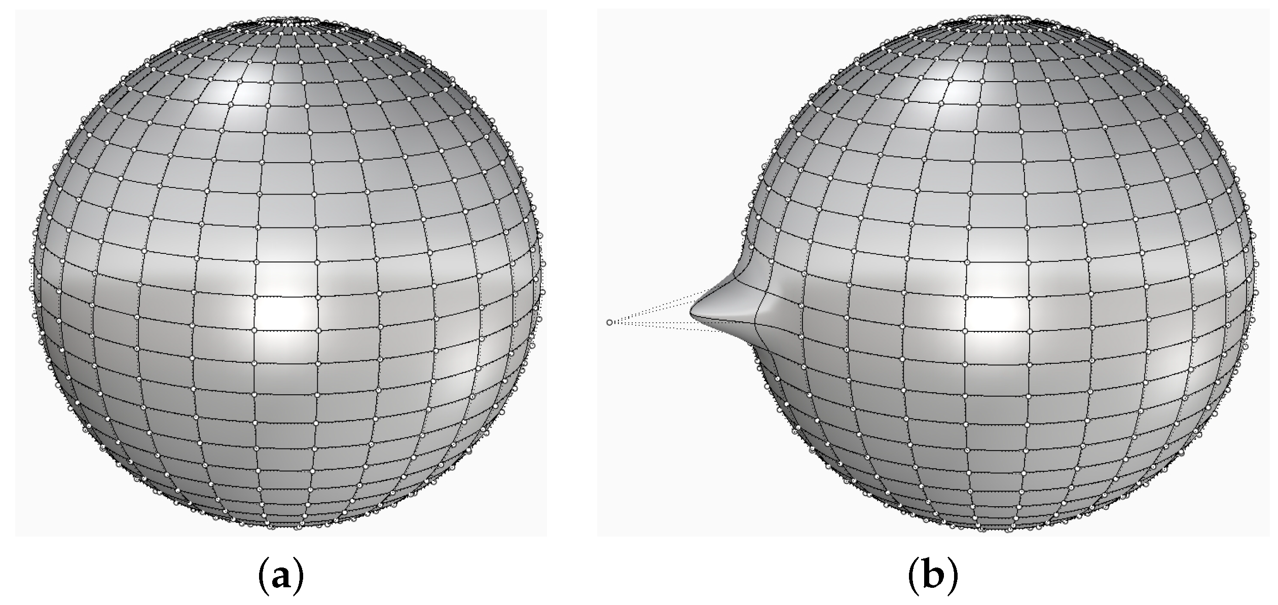
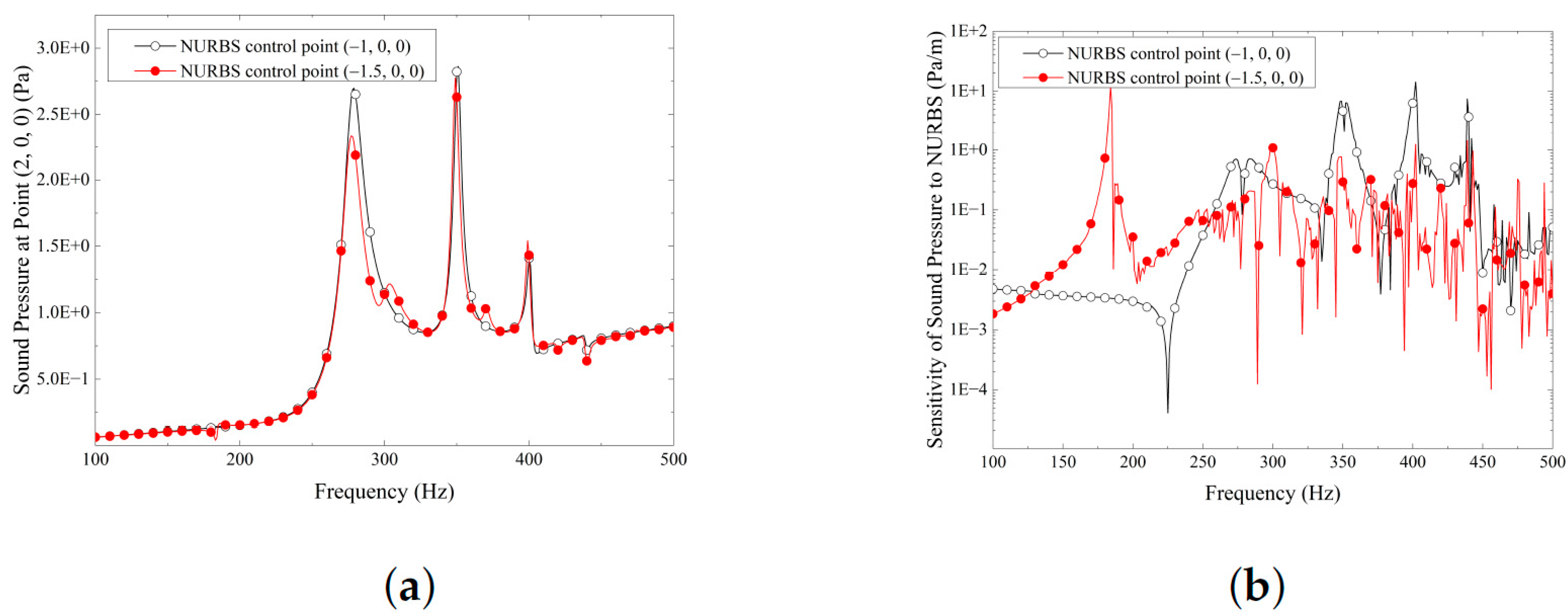
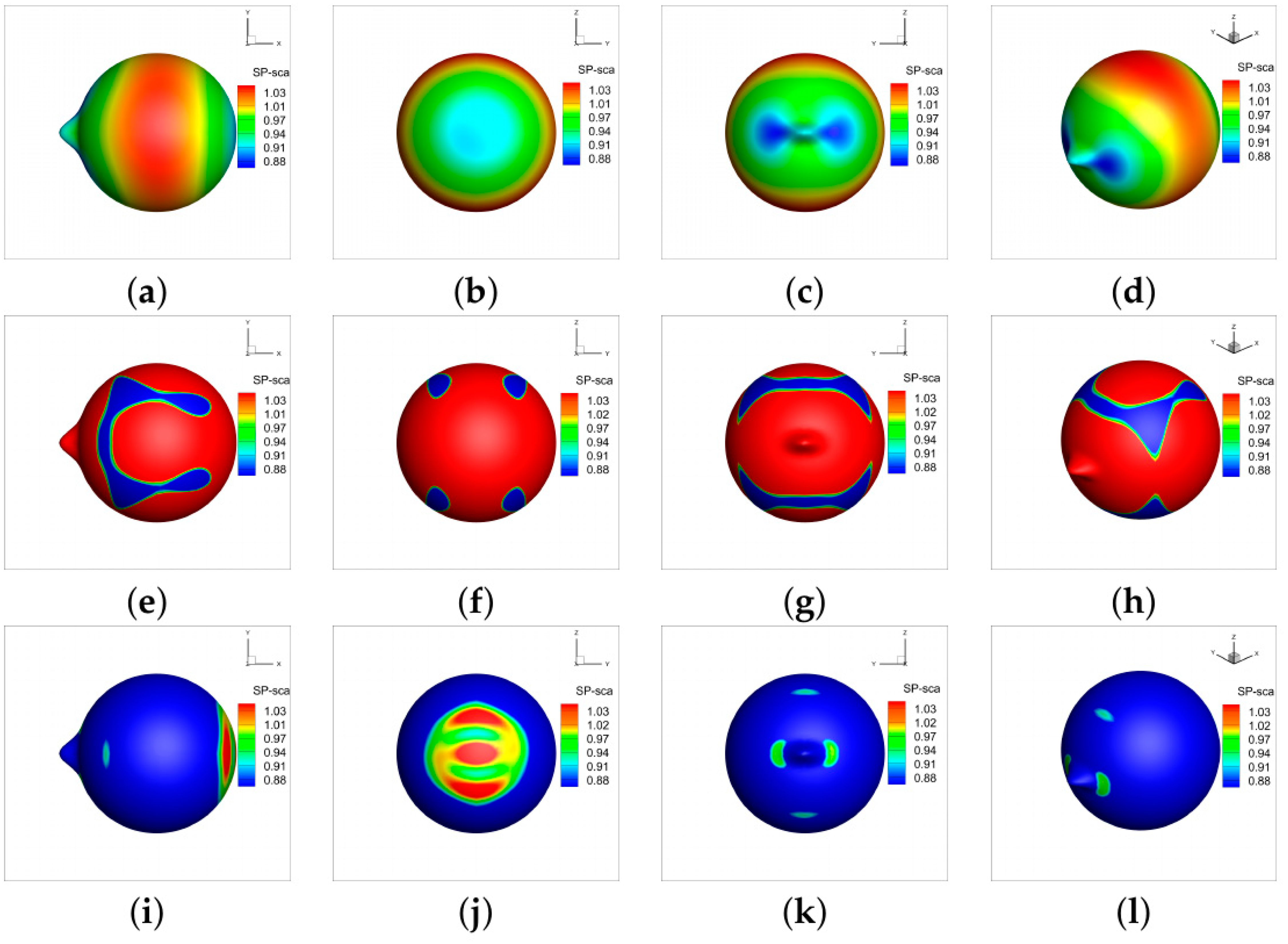
6.1. Spherical Models

Two different models of underwater, thin-pulsed shell are used in this subsection. The first is a simulation of a spherical outer shell with a 1.0 m radius, while the second is a similar shell with the NURBS control point $(-1,0,0)$ shifted to $(-1.5,0,0)$. The NURBS surface descriptions and accompanying control grids of these two models are shown in Figure 4. The fluid is water with density ${\rho }_f=1.0\times {10}^3$ $\mathrm{kg}/{\mathrm{m}}^3$, and the sound wave’s velocity in water is $c=1482$ $\mathrm{m}/\mathrm{s}$. The presented technique’s acoustic evaluation and shape sensitivity assessment are verified using the underwater, thin-pulsing, spherical surface example, as displayed in Figure 4a. While taking into consideration an incoming sound wave with an amplitude of $1.0$ in the positive x direction, the position $(0,0,0)$ is the center of the spherical shell.

Figure 5 gives the relative error of sound pressure between the numerical and analytical solutions, at point $(2,0,0)$ with a frequency at 200 Hz, for the spherical shell model shown in Figure 4a. As the total number of elements rises, the computational results converge quickly, as seen in Figure 5. Based on that, the total number of elements in the discretized thin-shell model is set to be 6144.

The outcomes are shown at location $(2,0,0)$ in Figure 6. Figure 7a displays the numerical and analytical results for the sound pressure at position $(2,0,0)$, respectively, presented in terms of frequencies. The FMM technique is used by GMRES implementation to speed up the linear solution. The conventional BEM’s exceptional accuracy is maintained by the FMM technique, as evidenced by the substantial concordance between the analytical and numerical outcomes in this figure.

Now, we go on to the investigation of shape sensitivity, which is crucial to shape optimization. In this case, at location $(2,0,0)$, the sound pressure serves as the objective function, and the x-coordinate at the control point $(-1,0,0)$ is the design variable. The sound pressure sensitivity is depicted in Figure 6b. Figure 6a,b illustrates how the sensitivity and pressure of the sound grows significantly at resonance peaks. The frequency range [100 Hz, 500 Hz] is crucial for this spherical shell model because there the sound pressure is noticeably greater and more variable to changes in the location of the previously mentioned NURBS point. In light of this finding, the frequency range used in the study of the spheroid-like shell problem is taken as [100 Hz, 500 Hz].

A spherical shell-like model may be obtained by moving the NURBS control point from its original location $(-1,0,0)$ to a new one $(-1.5,0,0)$, as illustrated in Figure 4b. The sound pressure at location $(2,0,0)$ for the spherical (as in Figure 4a) and spherical-like (NURBS control point $(-1,0,0)$ moved to $(-1.5,0,0)$, as in Figure 4b) thin-shell models are compared in Figure 7a. In Figure 7b, the sound pressure’s sensitivity at $(2,0,0)$ to the x-location of the NURBS control point $(-1.5,0,0)$ for the Figure 4b model is contrasted with that of the Figure 4a model. Basically, the results for these two models show a similar pattern. It should be observed that in Figure 7b, the extreme of sensitivity (the red line) for the model of Figure 4b occurs at the frequency of about 180 Hz, where the peak of the sound pressure resonance is not as high, as in Figure 7a. According to this phenomena, the highest resonance peak of sound pressure is not always where the bigger value of frequency sensitivity occurs. As a result, each sound pressure resonance peak should be taken into account when calculating sensitivity, necessitating a computation in terms of a frequency range.

Figure 8 shows the sound pressure on the spherical shell’s boundary surface at the frequencies of 100 Hz, 300 Hz, and 500 Hz. When the NURBS control point is moved from $(-1,0,0)$ to $(-1.5,0,0)$, Figure 9 gives the sound pressure on the shell’s boundary surface at the frequencies of 100 Hz, 300 Hz, and 500 Hz. Four ways of views are given for each calculation frequency. These figures show symmetrical features for both the $x-y$ and $x-z$ planes. Given that the plane wave occurs along with the x axis, these results make sense.

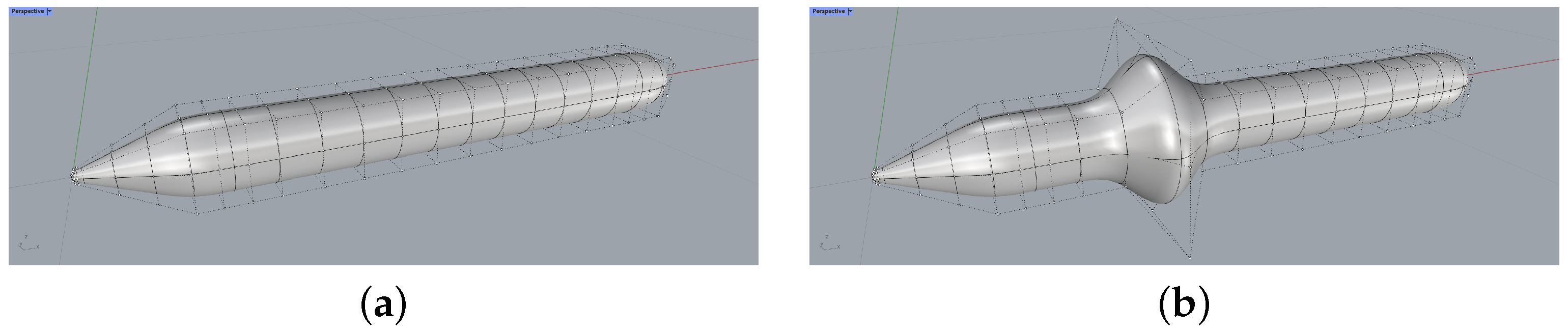
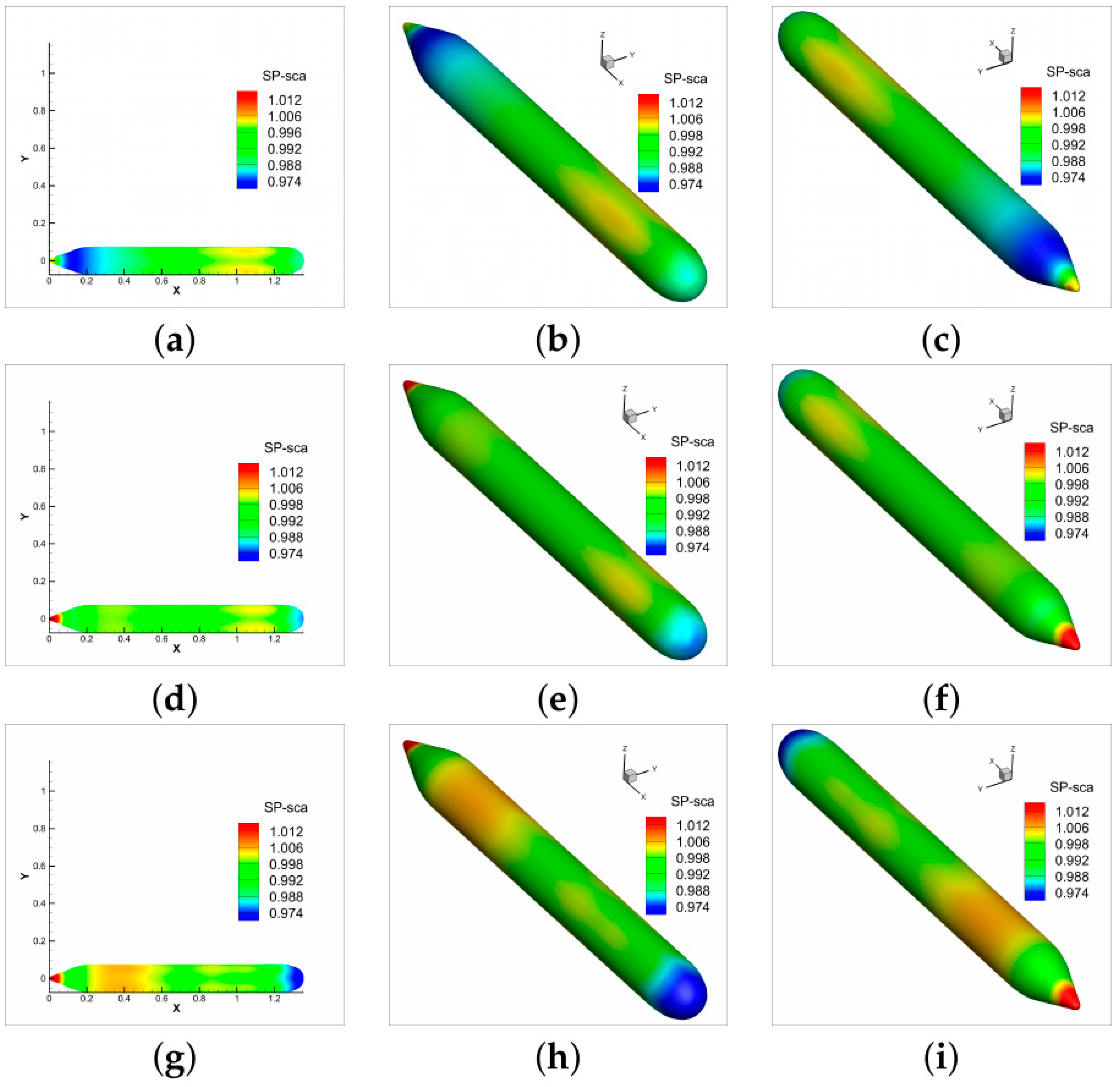
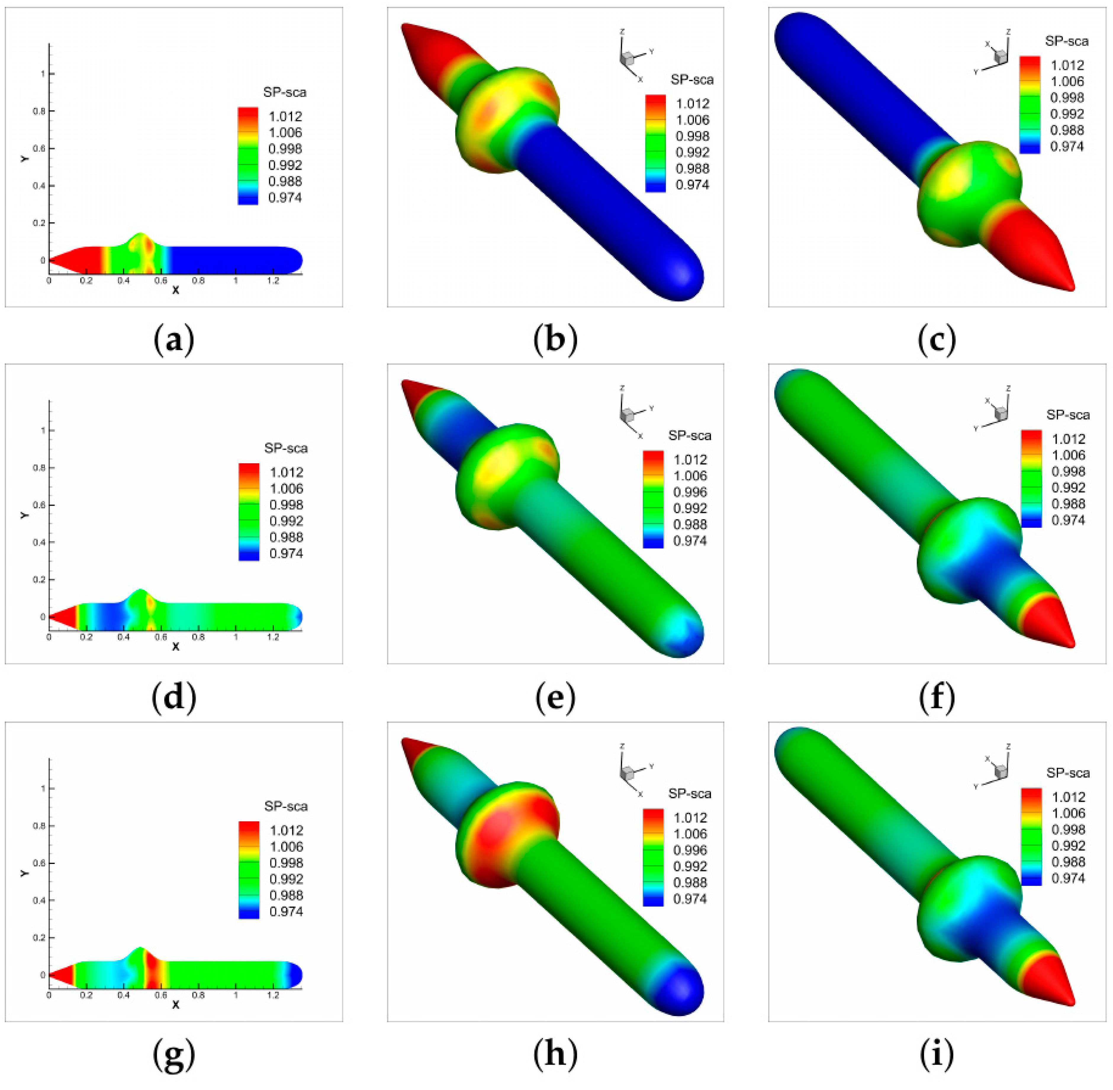
6.2. Submarine Model

This section uses two separate underwater, simplified, thin-walled submarine models, where the amplitude of the plane wave is $1.0$ and it propagates down the x axis in a positive direction, just as in the above numerical model. The left end control point of the first model, which is axially oriented along the x axis from left to right, as shown in Figure 10a, is situated at (0, 0, 0). The model consists of three sections and has a total length of approximately $1.35$ m. A conical surface is on the left, a cylindrical surface is in the middle, and a hemispherical surface is on the right. By extending the radius of a few of the cylinder surface’s NURBS control points in Figure 10a, a partly expanded simple submarine model may be produced, as seen in Figure 10b, where a circle of control points at x = 0.5 m is inflated to twice the radius.

Figure 11a, Figure 11c, and Figure 11e, respectively, give the sound pressure comparison at location (5, 0, 0), (20, 0, 0) and (100, 0, 0), for the models shown in Figure 10. The sound pressure’s sensitivity in relation to the cylinder’s radius at x = 0.5 m for these two models are given in Figure 11b (at point (5, 0, 0), the sound pressure is the objective function), Figure 11d (at point (20, 0, 0), the sound pressure is the objective function), and Figure 11f (at point (100, 0, 0), the sound pressure is the objective function). In these figures, sound pressure and sensitivity show a similar pattern of increasing and then decreasing. Additionally, the value of sound pressure and sensitivity decrease as the separation between the model and the computation point increases (calculation point from (5, 0, 0) to (100, 0, 0)). This outcome seems sensible given how energy decays.

The sound pressure on the model’s boundary surface in Figure 10a is displayed in Figure 12 at the frequency of 100 Hz, 300 Hz, and 500 Hz. For the model in Figure 10b, the sound pressure on the boundary surface is provided by Figure 13 at the frequencies of 100 Hz, 300 Hz, and 500 Hz. Three ways of view are given for each frequency. Considering that the plane wave moves in the direction of the x axis, the $x-y$ and $x-z$ planes’ symmetrical properties are depicted in these figures, just like in Figure 12 and Figure 13.

6.3. Fish Model

A simplified thin-shell fish model is given in this section to conduct sensitivity analysis. Similar to the submarine models, the outside load is the incident wave, which has an amplitude of $1.0$ and propagates down the x axis in a positive direction. Figure 14 shows the prototype example of the fish and its calculation model. The total length of the model is no more than 0.5 m and it keeps the basic shape of a manta ray. Due to the shape of the model, the calculation point is fixed at $(5,0,0)$. Furthermore, the variable thickness is chosen for sensitivity analysis and the value is set at 0.011 m.

Before giving the frequency scan figure, we calculate the sound pressure at a fixed frequency 200 Hz to verify the numerical method. Figure 15 gives the sound pressure distribution on the surface of the fish model, with a subfigure of real part (left) and a subfigure of imaginary part (right) of the sound pressure. From the figure, it can be seen that the sound pressure distributes in strips and shows a slowly decreasing trend along the direction of incidence; obviously, this result is from the model structure, as that the model itself is symmetric. Moreover, the maximum sound pressure of both the real and imaginary parts is around 1, which coincides with the magnitude of the external action. Thus, the figure proves the correctness of the numerical method intuitively.

Then, the sensitivity analysis was conducted using thickness as independent variable. A frequency scan with 0.011 m thickness and sensitivity to thickness are given in Figure 16. In Figure 16b, sound pressure and sensitivity shows a similar pattern of increasing and then decreasing. Here, we find that, in some frequency points, the sound pressure changes sharply and this also results in the sharp change in sensitivity. This kind of error is mainly caused by resonance phenomenon, and statistics of these points are not taken into consideration in this work. Thus, ignoring the resonance phenomenon, the outcome also seems reasonable and once again proves the effectiveness of our method.

The numerical simulations clearly show that the fluid effect needs to be considered while analyzing the vibro-acoustic radiation problem for underwater thin-shell constructions. Thus, it is necessary to perform the fluid–structure coupling analysis. Delineating high-quality meshes is crucial since the mesh quality has a direct impact on the computational correctness of the coupled analysis. This means that using IGA like NURBS to increase computational accuracy has significant benefits for both engineering and academia.

7. Conclusions

Sensitivity analysis and the modeling of the acoustic–structure interaction are conducted utilizing a coupling method grounded in the BEM and FEM. The structural elements of the problem are modeled using FEM. To avoid the necessity of meshing the acoustic space, the border of the structure being studied, which is also the acoustic domain’s border, is discretized using the BEM. To speed up the matrix-vector output, the FMM is employed. The utilisation of NURBS IGABEM enables the direct examination of the sensitivity of the structural–acoustic interaction using CAD models, without the necessity for meshing, thereby removing geometric mistakes. In coupling structural-acoustic systems, sound pressure sensitivity equations are created. Numerical examples are shown to demonstrate the accuracy and practicality of the proposed method. In real-world scenarios, the proposed method might be used to quantitatively predict how design elements would affect the sound field.

References

1. Junger, M.C.; Feit, D. Sound, Structures, and Their Interaction; MIT Press: Cambridge, MA, USA, 1986; Volume 225. [Google Scholar]
2. Sommerfeld, A. Partial Differential Equations in Physics; Academic Press: Cambridge, MA, USA, 1949; pp. v–vi. [Google Scholar] [CrossRef]
3. Engleder, S.; Steinbach, O. Stabilized boundary element methods for exterior Helmholtz problems. Numer. Math. 2008, 110, 145–160. [Google Scholar] [CrossRef]
4. Chen, L.; Zhang, Y.; Lian, H.; Atroshchenko, E.; Ding, C.; Bordas, S. Seamless integration of computer-aided geometric modeling and acoustic simulation: Isogeometric boundary element methods based on Catmull-Clark subdivision surfaces. Adv. Eng. Softw. 2020, 149, 102879. [Google Scholar] [CrossRef]
5. Everstine, G.C.; Henderson, F.M. Coupled finite element/boundary element approach for fluid-structure interaction. J. Acoust. Soc. Am. 1990, 87, 1938–1947. [Google Scholar] [CrossRef]
6. Fritze, D.; Marburg, S.; Hardtke, H.J. FEM-BEM-coupling and structural-acoustic sensitivity analysis for shell geometries. Comput. Struct. 2005, 83, 143–154. [Google Scholar] [CrossRef]
7. Martinsson, P.; Rokhlin, V. A fast direct solver for boundary integral equations in two dimensions. J. Comput. Phys. 2005, 205, 1–23. [Google Scholar] [CrossRef]
8. Martinsson, P.; Rokhlin, V. A fast direct solver for scattering problems involving elongated structures. J. Comput. Phys. 2007, 221, 288–302. [Google Scholar] [CrossRef]
9. Bebendorf, M. Rjasanow, S. Adaptive Low-Rank Approximation of Collocation Matrices. Computing 2003, 70, 1–24. [Google Scholar] [CrossRef]
10. Greengard, L.; Rokhlin, V. A fast algorithm for particle simulations. J. Comput. Phys. 1987, 73, 325–348. [Google Scholar] [CrossRef]
11. Coifman, R.; Rokhlin, V.; Wandzura, S. The fast multipole method for the wave equation: A pedestrian prescription. IEEE Antennas Propag. Mag. 1993, 35, 7–12. [Google Scholar] [CrossRef]
12. Rokhlin, V. Diagonal Forms of Translation Operators for the Helmholtz Equation in Three Dimensions. Appl. Comput. Harmon. Anal. 1993, 1, 82–93. [Google Scholar] [CrossRef]
13. Chen, L.; Marburg, S.; Zhao, W.; Liu, C.; Chen, H. Implementation of isogeometric fast multipole boundary element methods for 2D half-space acoustic scattering problems with absorbing boundary condition. J. Theor. Comput. Acoust. 2019, 27, 1850024. [Google Scholar] [CrossRef]
14. Chen, L.; Zhao, W.; Liu, C.; Chen, H.; Marburg, S. Isogeometric Fast Multipole Boundary Element Method Based on Burton-Miller Formulation for 3D Acoustic Problems. Arch. Acoust. 2019, 44, 475–492. [Google Scholar] [CrossRef]
15. Schneider, S. FE/FMBE coupling to model fluid-structure interaction. Int. J. Numer. Methods Eng. 2008, 76, 2137–2156. [Google Scholar] [CrossRef]
16. Kim, N.H.; Dong, J. Shape sensitivity analysis of sequential structural-acoustic problems using FEM and BEM. J. Sound Vib. 2006, 290, 192–208. [Google Scholar] [CrossRef]
17. Chen, L.; Zhao, J.; Lian, H.; Yu, B.; Atroshchenko, E.; Li, P. A BEM broadband topology optimization strategy based on Taylor expansion and SOAR method-Application to 2D acoustic scattering problems. Int. J. Numer. Methods Eng. 2023, 124, 5151–5182. [Google Scholar] [CrossRef]
18. Marburg, S. Developments in structural-acoustic optimization for passive noise control. Arch. Comput. Methods Eng. 2002, 9, 291–370. [Google Scholar] [CrossRef]
19. Lamancusa, J. Numerical optimization techniques for structural-acoustic design of rectangular panels. Comput. Struct. 1993, 48, 661–675. [Google Scholar] [CrossRef]
20. Hambric, S.A. Sensitivity Calculations for Broad-Band Acoustic Radiated Noise Design Optimization Problems. J. Vib. Acoust. 1996, 118, 529–532. [Google Scholar] [CrossRef]
21. Marburg, S.; Hardtke, H.J. Shape optimization of a vehicle hat-shelf: Improving acoustic properties for different load cases by maximizing first eigenfrequency. Comput. Struct. 2001, 79, 1943–1957. [Google Scholar] [CrossRef]
22. Choi, K.; Shim, I.; Wang, S. Design Sensitivity Analysis of Structure-Induced Noise and Vibration. J. Vib. Acoust. 1997, 119, 173–179. [Google Scholar] [CrossRef]
23. Wang, S. Design Sensitivity Analysis of Noise, Vibration, and Harshness of Vehicle Body Structure. Mech. Struct. Mach. 1999, 27, 317–335. [Google Scholar] [CrossRef]
24. Zheng, C.; Matsumoto, T.; Takahashi, T.; Chen, H. Explicit evaluation of hypersingular boundary integral equations for acoustic sensitivity analysis based on direct differentiation method. Eng. Anal. Bound. Elem. 2011, 35, 1225–1235. [Google Scholar] [CrossRef]
25. Simpson, R.; Bordas, S.; Trevelyan, J.; Rabczuk, T. A two-dimensional Isogeometric Boundary Element Method for elastostatic analysis. Comput. Methods Appl. Mech. Eng. 2012, 209–212, 87–100. [Google Scholar] [CrossRef]
26. Simpson, R.; Bordas, S.; Lian, H.; Trevelyan, J. An isogeometric boundary element method for elastostatic analysis: 2D implementation aspects. Comput. Struct. 2013, 118, 2–12. [Google Scholar] [CrossRef]
27. Hughes, T.; Cottrell, J.; Bazilevs, Y. Isogeometric analysis: CAD, finite elements, NURBS, exact geometry and mesh refinement. Comput. Methods Appl. Mech. Eng. 2005, 194, 4135–4195. [Google Scholar] [CrossRef]
28. Chen, L.; Lu, C.; Lian, H.; Liu, Z.; Zhao, W.; Li, S.; Chen, H.; Bordas, S.P. Acoustic topology optimization of sound absorbing materials directly from subdivision surfaces with isogeometric boundary element methods. Comput. Methods Appl. Mech. Eng. 2020, 362, 112806. [Google Scholar] [CrossRef]
29. Shen, X.; Du, C.; Jiang, S.; Sun, L.; Chen, L. Enhancing deep neural networks for multivariate uncertainty analysis of cracked structures by POD-RBF. Theor. Appl. Fract. Mech. 2023, 125, 103925. [Google Scholar] [CrossRef]
30. Scott, M.; Simpson, R.; Evans, J.; Lipton, S.; Bordas, S.; Hughes, T.; Sederberg, T. Isogeometric boundary element analysis using unstructured T-splines. Comput. Methods Appl. Mech. Eng. 2013, 254, 197–221. [Google Scholar] [CrossRef]
31. Takahashi, T.; Matsumoto, T. An application of fast multipole method to isogeometric boundary element method for Laplace equation in two dimensions. Eng. Anal. Bound. Elem. 2012, 36, 1766–1775. [Google Scholar] [CrossRef]
32. Chen, L.; Cheng, R.; Li, S.; Lian, H.; Zheng, C.; Bordas, S. A sample-efficient deep learning method for multivariate uncertainty qualification of acoustic-vibration interaction problems. Comput. Methods Appl. Mech. Eng. 2022, 393, 114784. [Google Scholar] [CrossRef]
33. Ginnis, A.; Kostas, K.; Politis, C.; Kaklis, P.; Belibassakis, K.; Gerostathis, T.; Scott, M.; Hughes, T. Isogeometric boundary-element analysis for the wave-resistance problem using T-splines. Comput. Methods Appl. Mech. Eng. 2014, 279, 425–439. [Google Scholar] [CrossRef]
34. Chen, L.; Lian, H.; Xu, Y.; Li, S.; Liu, Z.; Atroshchenko, E.; Kerfriden, P. Generalized isogeometric boundary element method for uncertainty analysis of time-harmonic wave propagation in infinite domains. Appl. Math. Model. 2023, 114, 360–378. [Google Scholar] [CrossRef]
35. Shen, X.; Du, C.; Jiang, S.; Zhang, P.; Chen, L. Multivariate uncertainty analysis of fracture problems through model order reduction accelerated SBFEM. Appl. Math. Model. 2024, 125, 218–240. [Google Scholar] [CrossRef]
36. Simpson, R.; Liu, Z.; Vázquez, R.; Evans, J. An isogeometric boundary element method for electromagnetic scattering with compatible B-spline discretizations. J. Comput. Phys. 2018, 362, 264–289. [Google Scholar] [CrossRef]
37. Xu, Y.; Li, H.; Chen, L.; Zhao, J.; Zhang, X. Monte Carlo Based Isogeometric Stochastic Finite Element Method for Uncertainty Quantization in Vibration Analysis of Piezoelectric Materials. Mathematics 2022, 10, 1840. [Google Scholar] [CrossRef]
38. Chen, L.; Wang, Z.; Lian, H.; Ma, Y.; Meng, Z.; Li, P.; Ding, C.; Bordas, S.P. Reduced order isogeometric boundary element methods for CAD-integrated shape optimization in electromagnetic scattering. Comput. Methods Appl. Mech. Eng. 2024, 419, 116654. [Google Scholar] [CrossRef]
39. Chen, L.; Liu, C.; Zhao, W.; Liu, L. An isogeometric approach of two dimensional acoustic design sensitivity analysis and topology optimization analysis for absorbing material distribution. Comput. Methods Appl. Mech. Eng. 2018, 336, 507–532. [Google Scholar] [CrossRef]
40. Xu, G.; Li, M.; Mourrain, B.; Rabczuk, T.; Xu, J.; Bordas, S.P. Constructing IGA-suitable planar parameterization from complex CAD boundary by domain partition and global/local optimization. Comput. Methods Appl. Mech. Eng. 2018, 328, 175–200. [Google Scholar] [CrossRef]
41. Li, S.; Trevelyan, J.; Wu, Z.; Lian, H.; Wang, D.; Zhang, W. An adaptive SVD-Krylov reduced order model for surrogate based structural shape optimization through isogeometric boundary element method. Comput. Methods Appl. Mech. Eng. 2019, 349, 312–338. [Google Scholar] [CrossRef]
42. Chen, L.; Lian, H.; Liu, Z.; Chen, H.; Atroshchenko, E.; Bordas, S. Structural shape optimization of three dimensional acoustic problems with isogeometric boundary element methods. Comput. Methods Appl. Mech. Eng. 2019, 355, 926–951. [Google Scholar] [CrossRef]
43. Lian, H.; Chen, L.; Lin, X.; Zhao, W.; Bordas, S.P.A.; Zhou, M. Noise Pollution Reduction through a Novel Optimization Procedure in Passive Control Methods. Comput. Model. Eng. Sci. 2022, 131, 1–18. [Google Scholar] [CrossRef]
44. Chen, L.; Lian, H.; Natarajan, S.; Zhao, W.; Chen, X.; Bordas, S. Multi-frequency acoustic topology optimization of sound-absorption materials with isogeometric boundary element methods accelerated by frequency-decoupling and model order reduction techniques. Comput. Methods Appl. Mech. Eng. 2022, 395, 114997. [Google Scholar] [CrossRef]
45. Chen, L.; Li, K.; Peng, X.; Lian, H.; Lin, X.; Fu, Z. Isogeometric Boundary Element Analysis for 2D Transient Heat Conduction Problem with Radial Integration Method. CMES-Comput. Model. Eng. Sci. 2021, 126, 125–146. [Google Scholar] [CrossRef]
46. Chen, L.; Li, H.; Guo, Y.; Chen, P.; Atroshchenko, E.; Lian, H. Uncertainty quantification of mechanical property of piezoelectric materials based on isogeometric stochastic FEM with generalized n th-order perturbation. Eng. Comput. 2023, 1–21. [Google Scholar] [CrossRef]
47. Rehman, F.U.; Huang, L.; Anderlini, E.; Thomas, G. Hydrodynamic Modelling for a Transportation System of Two Unmanned Underwater Vehicles: Semi-Empirical, Numerical and Experimental Analyses. J. Mar. Sci. Eng. 2021, 9, 500. [Google Scholar] [CrossRef]
48. Burton, A.J.; Miller, G.F. The Application of Integral Equation Methods to the Numerical Solution of Some Exterior Boundary-Value Problems. Proc. R. Soc. Lond. 1971, 323, 201–210. [Google Scholar] [CrossRef]
49. Ciskowski, R.D.; Brebbia, C.A. Boundary Element Methods in Acoustics; Springer: Berlin/Heidelberg, Germany, 1991. [Google Scholar]
50. Marjan, A.; Huang, L. Topology optimisation of offshore wind turbine jacket foundation for fatigue life and mass reduction. Ocean. Eng. 2023, 289, 116228. [Google Scholar] [CrossRef]
51. Huang, L.; Pena, B.; Liu, Y.; Anderlini, E. Machine learning in sustainable ship design and operation: A review. Ocean. Eng. 2022, 266, 112907. [Google Scholar] [CrossRef]
52. Chen, L.; Lian, H.; Liu, Z.; Gong, Y.; Zheng, C.; Bordas, S. Bi-material topology optimization for fully coupled structural-acoustic systems with isogeometric FEM-BEM. Eng. Anal. Bound. Elem. 2022, 135, 182–195. [Google Scholar] [CrossRef]
53. Zheng, C.; Matsumoto, T.; Takahashi, T.; Chen, H. A wideband fast multipole boundary element method for three dimensional acoustic shape sensitivity analysis based on direct differentiation method. Eng. Anal. Bound. Elem. 2012, 36, 361–371. [Google Scholar] [CrossRef]
Figure 1. Knot vector {0, 0, 0, 0, 1, 2, 3, 4, 4, 4, 4}.
Jmse 12 00098 g001
Figure 2. NURBS basis functions.
Jmse 12 00098 g002
Figure 3. NURBS geometries. (a) NURBS curve; (b) NURBS surface.
Jmse 12 00098 g003
Figure 4. Control points distribution in the NURBS models of pulsing sphere. (a) The NURBS model of pulsing sphere. (b) The NURBS model of pulsing sphere, with the control point (−1, 0, 0) moved to (−1.5, 0, 0).
Jmse 12 00098 g004
Figure 5. The relative error of sound pressure between the numerical and analytical solutions, at point  ( 2 , 0 , 0 )  with frequency at 200 Hz, for the spherical shell model shown in Figure 4a.
Jmse 12 00098 g005
Figure 6. Sound pressure and sensitivity at point  ( 2 , 0 , 0 )  for spherical shell model. (a) Spherical shell model, sound pressure at point  ( 2 , 0 , 0 ) . (b) Spherical shell model, sound pressure’s sensitivity at point  ( 2 , 0 , 0 )  to NURBS coordinate.
Jmse 12 00098 g006
Figure 7. NURBS coordinate  ( 1 , 0 , 0 )  vs.  ( 1.5 , 0 , 0 ) , sound pressure and sensitivity at point  ( 2 , 0 , 0 )  for thin-shell model. (a) NURBS coordinate  ( 1 , 0 , 0 )  vs.  ( 1.5 , 0 , 0 ) , sound pressure at point  ( 2 , 0 , 0 ) . (b) NURBS coordinate  ( 1 , 0 , 0 )  vs.  ( 1.5 , 0 , 0 ) , sound pressure’s sensitivity at point  ( 2 , 0 , 0 )  to NURBS coordinate.
Jmse 12 00098 g007
Figure 8. Sound pressure on the spherical shell’s boundary surface at a frequency of 100 Hz (the top row), 300 Hz (the middle row), and 500 Hz (the bottom row). (a) View along the  z  axis. (b) View along the  x  axis. (c) View along the x axis. (d) View in the direction of (1, 1, −1). (e) View along the  z  axis. (f) View along the  x  axis. (g) View along the x axis. (h) View in the direction of (1, 1, −1). (i) View along the  z  axis. (j) View along the  x  axis. (k) View along the x axis. (l) View in the direction of (1, 1, −1).
Jmse 12 00098 g008
Figure 9. Sound pressure on the spherical shell’s boundary surface at a frequency of 100 Hz (the top row), 300 Hz (the middle row), and 500 Hz (the bottom row), with the NURBS control point  ( 1 , 0 , 0 )  moved to  ( 1.5 , 0 , 0 ) . (a) View along the  z  axis. (b) View along the  x  axis. (c) View along the x axis. (d) View in the direction of (1, 1, −1). (e) View along the  z  axis. (f) View along the  x  axis. (g) View along the x axis. (h) View in the direction of (1, 1, −1). (i) View along the  z  axis. (j) View along the  x  axis. (k) View along the x axis. (l) View in the direction of (1, 1, −1).
Jmse 12 00098 g009
Figure 10. Control points distribution in the NURBS models of simple submarine. The left end control point is situated at  ( 0 , 0 , 0 ) . The positive direction of the x axis is from the model’s left end to its right endpoint. (a) The NURBS model of a simple submarine. (b) The NURBS model of a partly expanded simple submarine.
Jmse 12 00098 g010
Figure 11. Sound pressure and sensitivity at point  ( 5 , 0 , 0 ) ( 20 , 0 , 0 ) , and  ( 100 , 0 , 0 )  for submarine models. (a) Simple submarine vs. partly expanded simple submarine model, sound pressure at point  ( 5 , 0 , 0 ) . (b) Simple submarine vs. partly expanded simple submarine model, sound pressure’s sensitivity at point  ( 5 , 0 , 0 )  to NURBS coordinate. (c) Simple submarine vs. partly expanded simple submarine model, sound pressure at point  ( 20 , 0 , 0 ) . (d) Simple submarine vs. partly expanded simple submarine model, sound pressure’s sensitivity at point  ( 20 , 0 , 0 )  to NURBS coordinate. (e) Simple submarine vs. partly expanded simple submarine model, sound pressure at point  ( 100 , 0 , 0 ) . (f) Simple submarine vs. partly expanded simple submarine model, sound pressure’s sensitivity at point  ( 100 , 0 , 0 )  to NURBS coordinate.
Jmse 12 00098 g011aJmse 12 00098 g011b
Figure 12. Sound pressure on the simple submarine’s boundary surface at a frequency of 100 Hz (the top row), 300 Hz (the middle row), and 500 Hz (the bottom row). (a) 2D view. (b) 3D view in the direction of (−1, 1, −1). (c) 3D view in the direction of (1, −1, −1). (d) 2D view. (e) 3D view in the direction of (−1, 1, −1). (f) 3D view in the direction of (1, −1, −1). (g) 2D view. (h) 3D view in the direction of (−1, 1, −1). (i) 3D view in the direction of (1, −1, −1).
Jmse 12 00098 g012
Figure 13. Sound pressure on the partly expanded simple submarine’s boundary surface at a frequency of 100 Hz (the top row), 300 Hz (the middle row), and 500 Hz (the bottom row). (a) 2D view. (b) 3D view in the direction of (−1, 1, −1). (c) 3D view in the direction of (1, −1, −1). (d) 2D view. (e) 3D view in the direction of (−1, 1, −1). (f) 3D view in the direction of (1, −1, −1). (g) 2D view. (h) 3D view in the direction of (−1, 1, −1). (i) 3D view in the direction of (1, −1, −1).
Jmse 12 00098 g013
Figure 14. Robot fish and calculation model. (a) Robot 1. (b) Scale. (c) Model. (d) Mesh.
Jmse 12 00098 g014
Figure 15. Sound pressure distribution on model surface at 200 Hz, thickness = 0.011 m.
Jmse 12 00098 g015
Figure 16. Sound pressure and sensitivity analysis of fish model. (a) Sound pressure at  ( 5 , 0 , 0 ) , thickness =  0.011  m. (b) Sensitivity of sound pressure to thickness, at point  ( 5 , 0 , 0 ) .
Jmse 12 00098 g016
Disclaimer/Publisher’s Note: The statements, opinions and data contained in all publications are solely those of the individual author(s) and contributor(s) and not of MDPI and/or the editor(s). MDPI and/or the editor(s) disclaim responsibility for any injury to people or property resulting from any ideas, methods, instructions or products referred to in the content.