

Research on Obstacle Avoidance Planning for UUV Based on A3C Algorithm

 , , ,
, , ,
Abstract
:1. Introduction
2. Materials
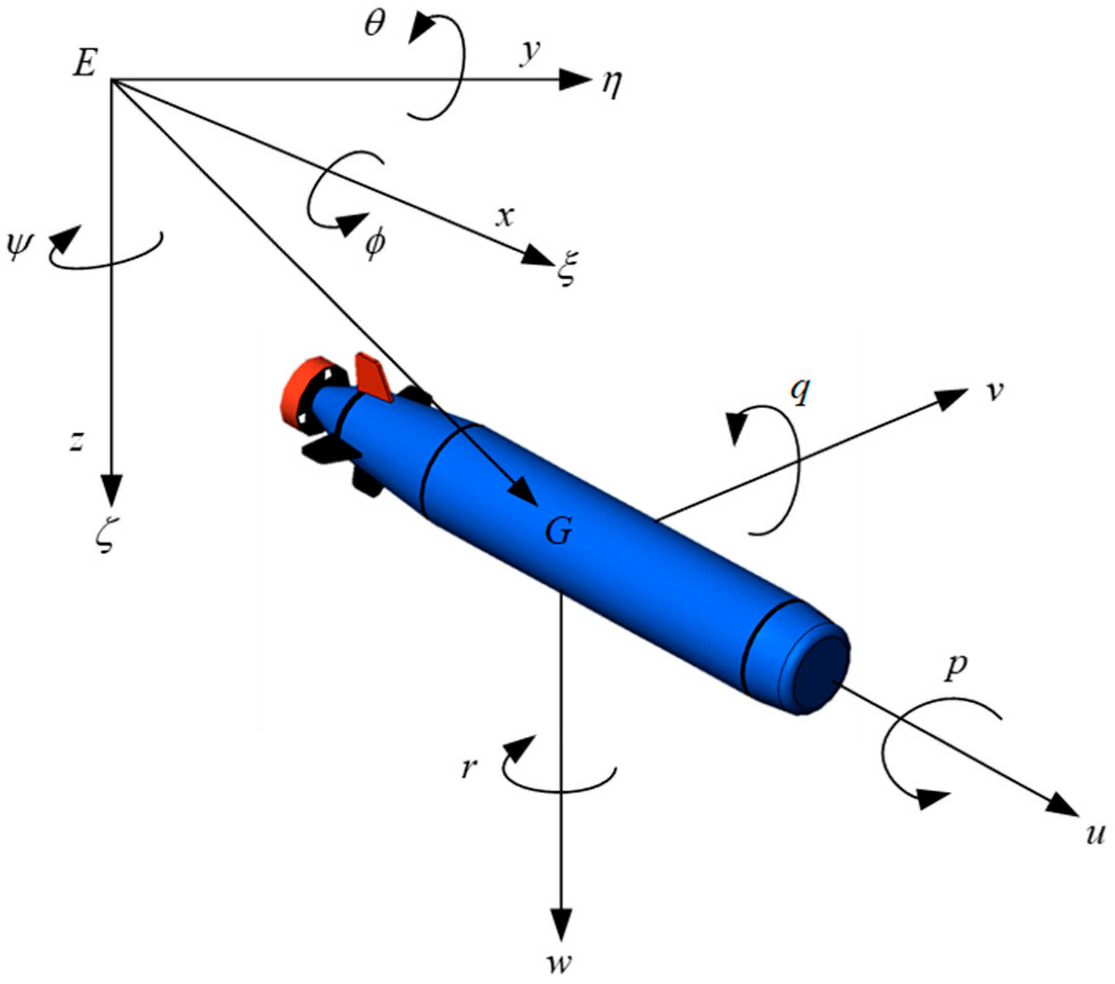
2.1. UUV Model
- (1)
- Neglecting the influence of third-order and higher-order hydrodynamic coefficients on the UUV;
- (2)
- Neglecting the influence of roll, pitch, and heave movements of the UUV on horizontal motion.
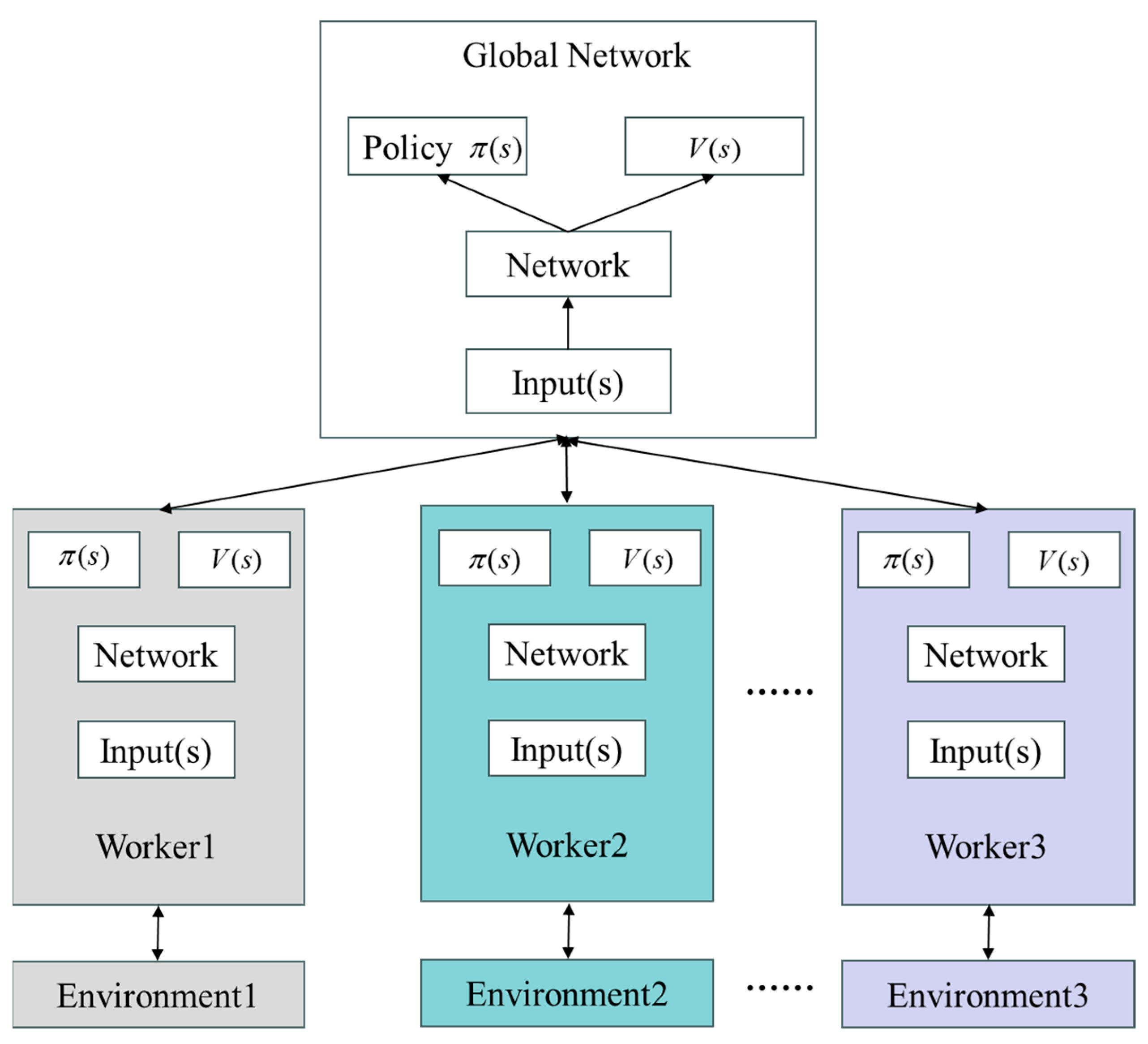
2.2. A3C
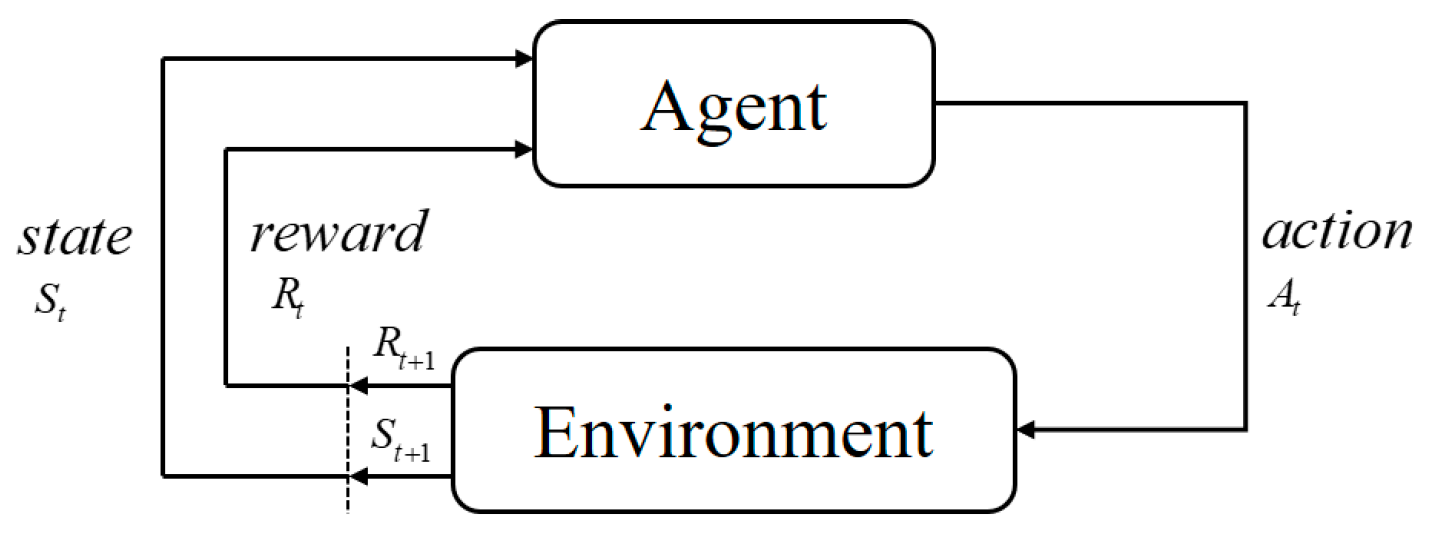
2.2.1. Reinforcement Learning
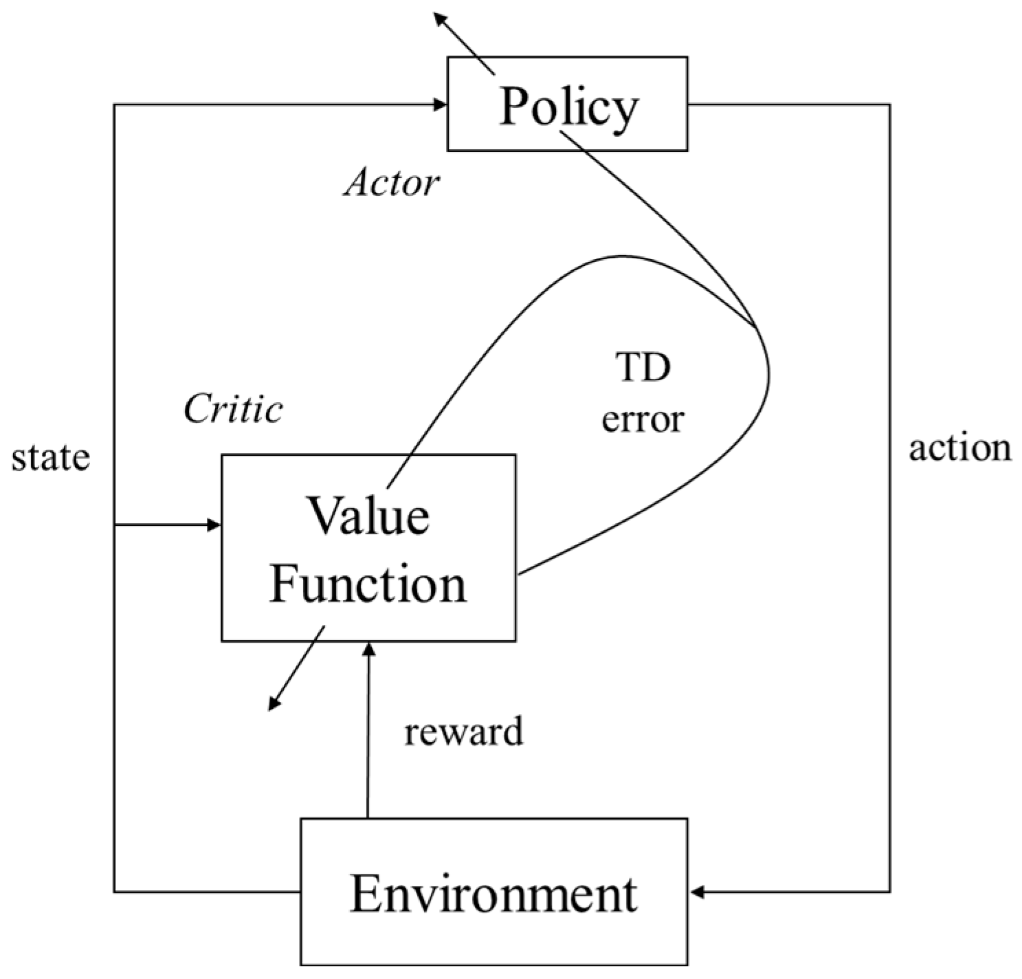
2.2.2. A3C
| Algorithm 1 A3C |
| // Assume global shared parameter vectors and and global shared counter T = 0 |
| // Assume thread-specific parameter vectors and |
| Initialize thread step counter t 1 |
| repeat |
| Reset gradients: and . |
| Synchronize thread-specific parameters and |
| Get state |
| repeat |
| Perform according to policy |
| Receive reward and new state |
| until terminal or |
| for do |
| Accumulate gradients wrt : |
| Accumulate gradients wrt : |
| end for |
| Perform asynchronous update of using and of using d |
| until |
3. The A3C Collision Avoidance Planning Algorithm
3.1. State Space
3.2. Action Space
3.3. Reward Function
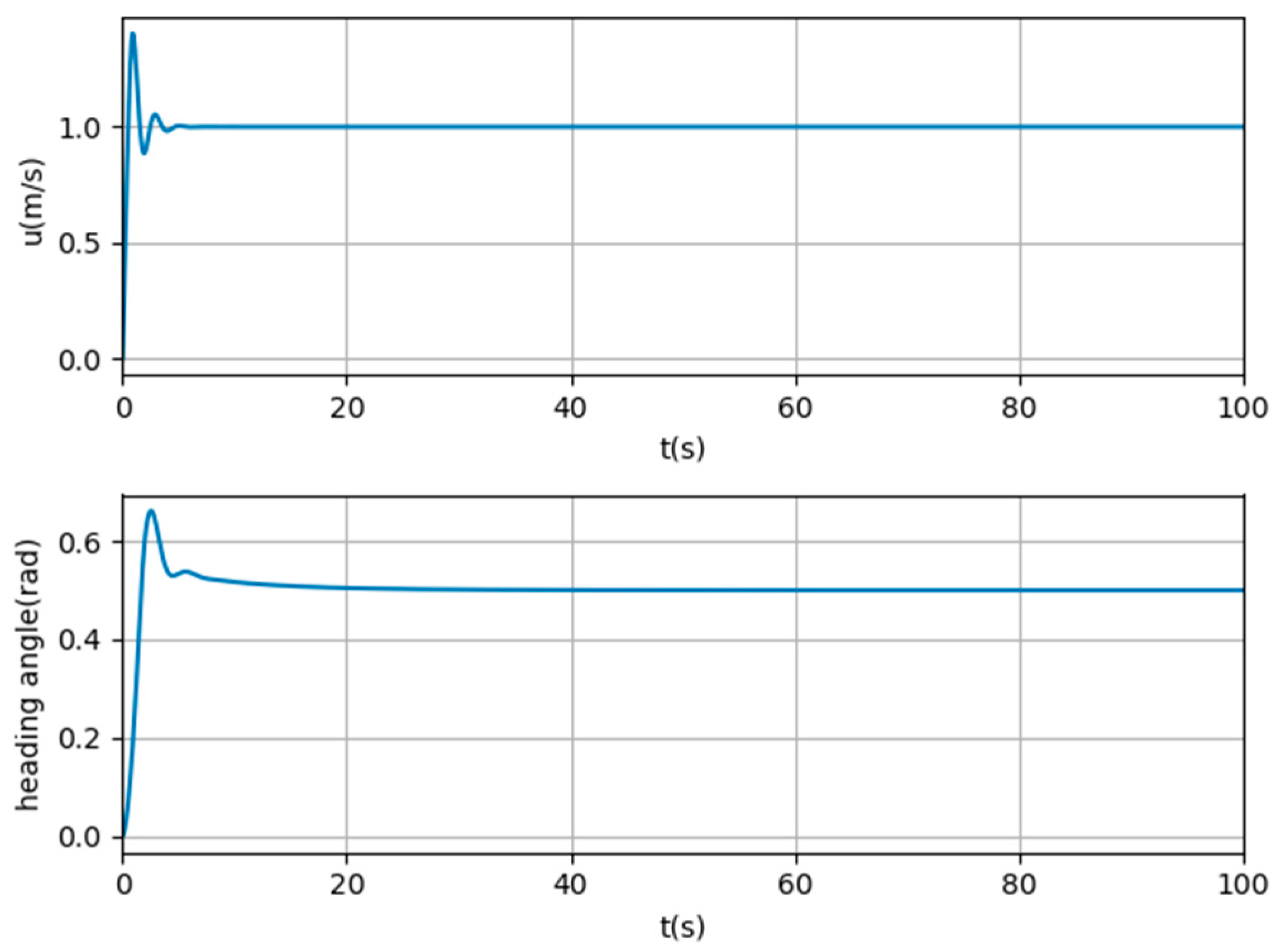
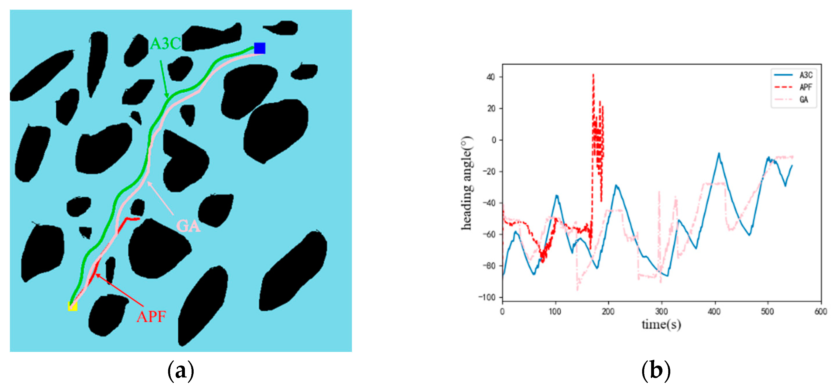
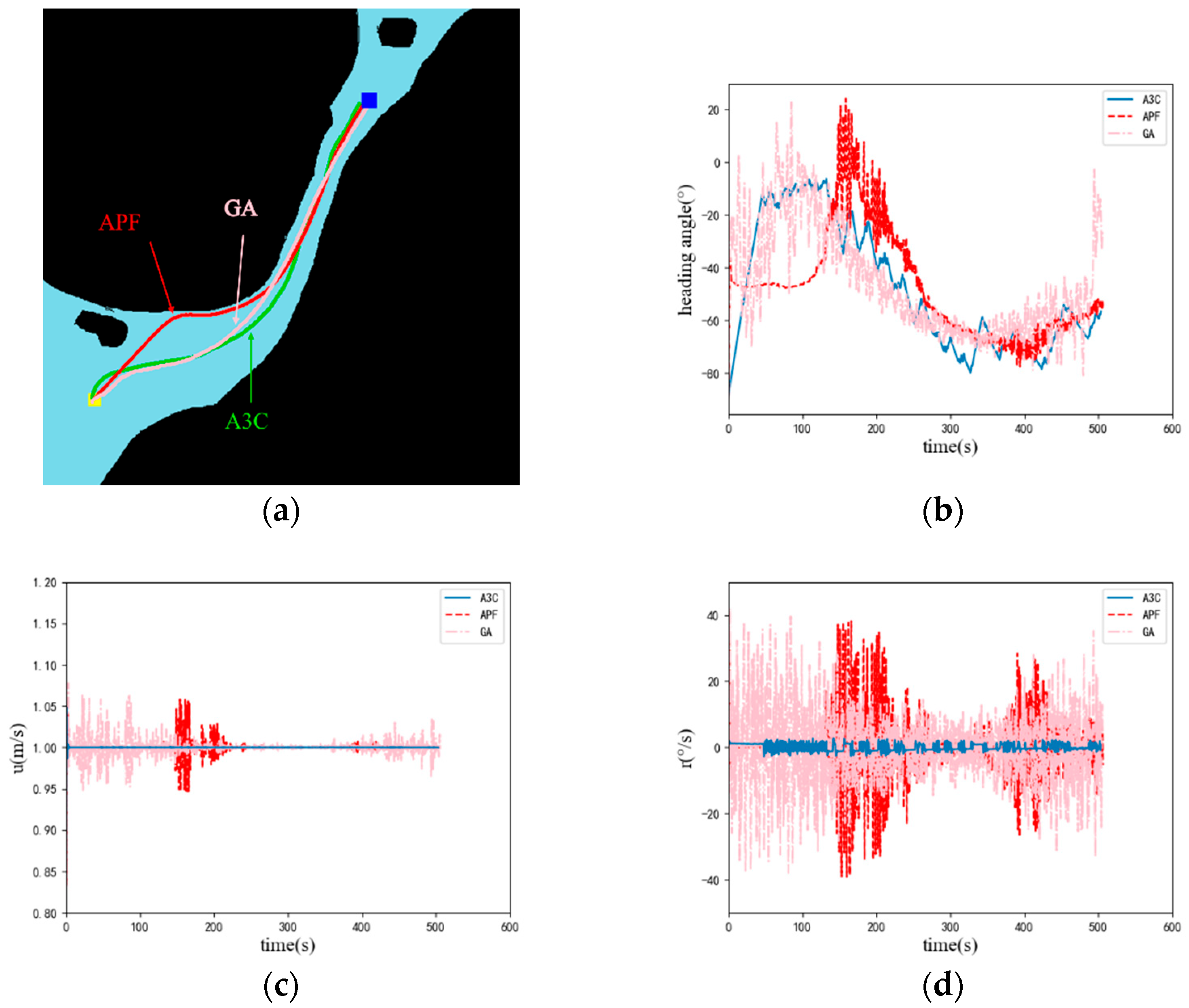
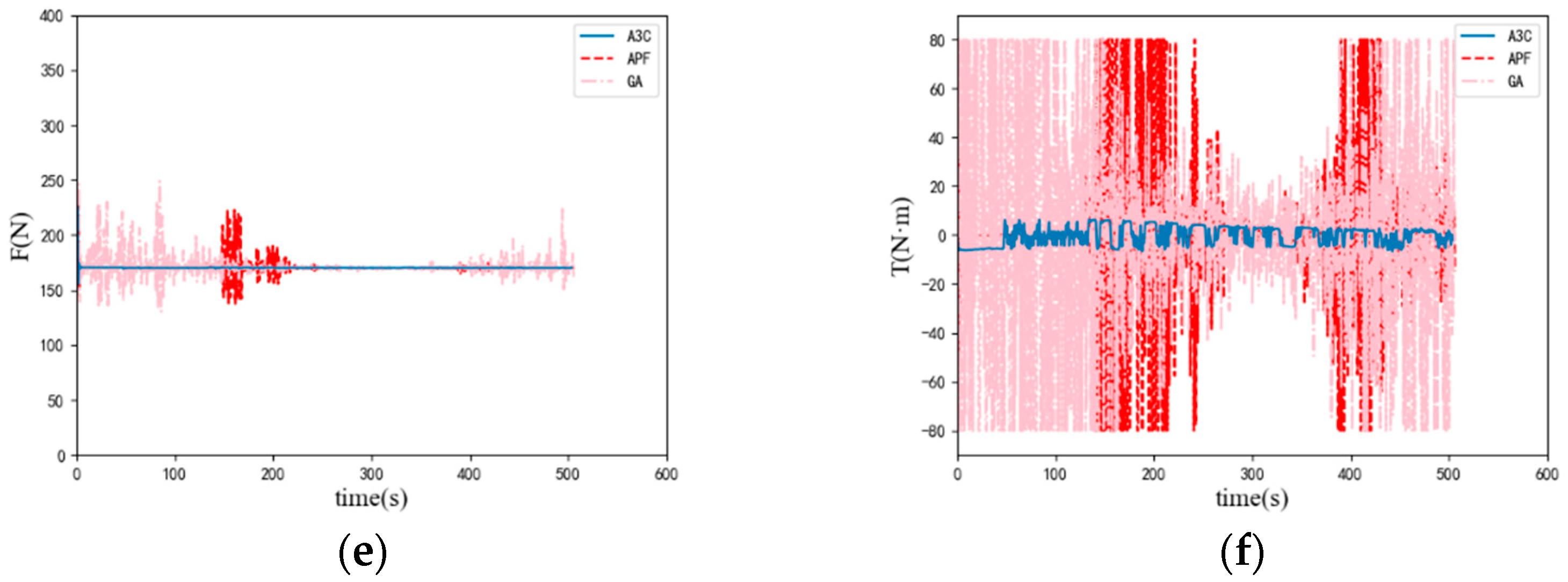
4. Experiments and Results
5. Conclusions
Author Contributions
Funding
Institutional Review Board Statement
Informed Consent Statement
Data Availability Statement
Acknowledgments
Conflicts of Interest
References
- Zhu, D.; Yang, S.X. Bio-Inspired Neural Network-Based Optimal Path Planning for UUVs Under the Effect of Ocean Currents. IEEE Trans. Intell. Veh. 2021, 7, 231–239. [Google Scholar] [CrossRef]
- Yue, Y.; Hao, W.; Guanjie, H.; Yao, Y. UUV Target Tracking Path Planning Algorithm Based on Deep Reinforcement Learning. In Proceedings of the 2023 8th Asia-Pacific Conference on Intelligent Robot Systems (ACIRS), Xi’an, China, 7–9 July 2023; pp. 65–71. [Google Scholar]
- Li, D.; Wang, P.; Du, L. Path Planning Technologies for Autonomous Underwater Vehicles-A Review. IEEE Access 2019, 7, 9745–9768. [Google Scholar] [CrossRef]
- Cai, Y.; Zhang, E.; Qi, Y.; Lu, L. A Review of Research on the Application of Deep Reinforcement Learning in Unmanned Aerial Vehicle Resource Allocation and Trajectory Planning. In Proceedings of the 2022 4th International Conference on Machine Learning, Big Data and Business Intelligence (MLBDBI), Shanghai, China, 28–30 October 2022; pp. 238–241. [Google Scholar]
- Zhu, K.; Zhang, T. Deep reinforcement learning based mobile robot navigation: A review. Tsinghua Sci. Technol. 2021, 26, 674–691. [Google Scholar] [CrossRef]
- Lample, G.; Chaplot, D.S. Playing FPS Games with Deep Reinforcement Learning. arXiv 2016, arXiv:1609.05521. [Google Scholar] [CrossRef]
- Mnih, V.; Kavukcuoglu, K.; Silver, D.; Graves, A.; Antonoglou, I.; Wierstra, D.; Riedmiller, M. Playing Atari with Deep Reinforcement Learning. Comput. Sci. 2013, 201–220. [Google Scholar] [CrossRef]
- Mnih, V.; Kavukcuoglu, K.; Silver, D.; Rusu, A.A.; Veness, J.; Bellemare, M.G.; Graves, A.; Riedmiller, M.; Fidjeland, A.K.; Ostrovski, G.; et al. Human-level control through deep reinforcement learning. Nature 2015, 518, 529–533. [Google Scholar] [CrossRef] [PubMed]
- Wang, Z.; Schaul, T.; Hessel, M.; Hasselt, H.; Lanctot, M.; Freitas, N. Dueling network architectures for deep reinforcement learning. Proc. Mach. Learn. Res. 2015, 48, 1995–2003. [Google Scholar]
- Hasselt, H.V.; Guez, A.; Hessel, M.; Mnih, V.; Silver, D. Learning functions across many orders of magnitudes. arXiv 2016, arXiv:1602.07714. [Google Scholar]
- Lillicrap, T.; Hunt, J.; Pritzel, A.; Heess, N.; Erez, T.; Tassa, Y.; Silver, D.; Wierstra, D. Continuous control with deep reinforcement learning. arXiv 2015, arXiv:1509.02971. [Google Scholar]
- Mnih, V.; Badia, A.P.; Mirza, M.; Graves, A.; Lillicrap, T.P.; Harley, T.; Silver, D.; Kavukcuoglu, K. Asynchronous Methods for Deep Reinforcement Learning. arXiv 2016, arXiv:1602.01783. [Google Scholar]
- Dobrevski, M.; Skočaj, D. Adaptive Dynamic Window Approach for Local Navigation. In Proceedings of the 2020 IEEE/RSJ International Conference on Intelligent Robots and Systems (IROS), Las Vegas, NV, USA, 24 October 2020–24 January 2021; pp. 6930–6936. [Google Scholar]
- Rodriguez, S.; Tang, X.; Lien, J.-M.; Amato, N.M. An Obstacle-based Rapidly-exploring Random Tree. In Proceedings of the 2006 IEEE International Conference on Robotics and Automation, Orlando, FL, USA, 15–19 May 2006; pp. 895–900. [Google Scholar]
- Igarashi, H.; Kakikura, M. Path and Posture Planning for Walking Robots by Artificial Potential Field Method. In Proceedings of the IEEE International Conference on Robotics and Automation, New Orleans, LA, USA, 26 April–1 May 2004. [Google Scholar]
- Hu, Y.; Yang, S.X. A Knowledge Based Genetic Algorithm for Path Planning of a Mobile Robot. In Proceedings of the IEEE International Conference on Robotics and Automation, New Orleans, LA, USA, 26 April–1 May 2004. [Google Scholar]
- Kennedy, J.; Eberhart, R. Particle Swarm Optimization. In Proceedings of the 1995 IEEE International Conference, Perth, WA, Australia, 27 November–1 December 1995; pp. 1942–1948. [Google Scholar]
- Li, S.; Su, W.; Huang, R.; Zhang, S. Mobile Robot Navigation Algorithm Based on Ant Colony Algorithm with A* Heuristic Method. In Proceedings of the 2020 4th International Conference on Robotics and Automation Sciences, Wuhan, China, 12–14 June 2020; pp. 28–33. [Google Scholar]
- Tang, B.; Zhanxia, Z.; Luo, J. A Convergence-guaranteed Particle Swarm Optimization Method for Mobile Robot Global Path Planning. Assem. Autom. 2017, 37, 114–129. [Google Scholar] [CrossRef]
- Lin, C.; Wang, H.; Yuan, J.; Yu, D.; Li, C. An Improved Recurrent Neural Network for Unmanned Underwater Vehicle Online Obstacle Avoidance. Ocean Eng. 2019, 189, 106327. [Google Scholar] [CrossRef]
- Bhopale, P.; Kazi, F.; Singh, N. Reinforcement Learning Based Obstacle Avoidance for Autonomous Underwater Vehicle. J. Mar. Sci. Appl. 2019, 18, 228–238. [Google Scholar] [CrossRef]
- Wang, J.; Lei, G.; Zhang, J. Study of UAV Path Planning Problem Based on DQN and Artificial Potential Field Method. In Proceedings of the 2023 4th International Symposium on Computer Engineering and Intelligent Communications, Nanjing, China, 18–20 August 2023; pp. 175–182. [Google Scholar]
- Bodaragama, J.; Rajapaksha, U.U.S. Path Planning for Moving Robots in an Unknown Dynamic Area Using RND-Based Deep Reinforcement Learning. In Proceedings of the 2023 3rd International Conference on Advanced Research in Computing (ICARC), Belihuloya, Sri Lanka, 23–24 February 2023; pp. 13–18. [Google Scholar]
- Sasaki, Y.; Matsuo, S.; Kanezaki, A.; Takemura, H. A3C Based Motion Learning for an Autonomous Mobile Robot in Crowds. In Proceedings of the 2019 IEEE International Conference on Systems, Man and Cybernetics (SMC), Bari, Italy, 6–9 October 2019. [Google Scholar]
- Zhou, Z.; Zheng, Y.; Liu, K.; He, X.; Qu, C. A Real-time Algorithm for USV Navigation Based on Deep Reinforcement Learning. In Proceedings of the 2019 IEEE International Conference on Signal, Information and Data Processing (ICSIDP), Chongqing, China, 11–13 December 2019; pp. 1–4. [Google Scholar]
- Lapierre, L.; Soetanto, D. Nonlinear path-following control of an AUV. Ocean Eng. 2007, 34, 1734–1744. [Google Scholar] [CrossRef]
- White III, C.C.; White, D.J. Markov Decision Process. Eur. J. Oper. Res. 1989, 39, 1–16. [Google Scholar] [CrossRef]
- Siraskar, R.; Kumar, S.; Patil, S.; Bongale, A.; Kotecha, K. Reinforcement learning for predictive maintenance: A systematic technical review. Artif. Intell. Rev. 2023, 56, 12885–12947. [Google Scholar] [CrossRef]
- Yu, K.; Jin, K.; Deng, X. Review of Deep Reinforcement Learning. In Proceedings of the 2022 IEEE 5th Advanced Information Management, Communicates, Electronic and Automation Control Conference (IMCEC), Chongqing, China, 16–18 December 2022; pp. 41–48. [Google Scholar]
- Peters, J.; Schaal, S. Natural actor-critic. Neurocomputing 2008, 71, 1180–1190. [Google Scholar] [CrossRef]
- Bhatnagar, S.; Sutton, R.S.; Ghavamzadeh, M.; Lee, M. Natural actor–critic algorithms. Automatica 2009, 45, 2471–2482. [Google Scholar] [CrossRef]
- Chen, T.; Liu, J.Q.; Li, H.; Wang, S.R.; Niu, W.J.; Tong, E.D.; Chang, L.; Chen, Q.A.; Li, G. Robustness Assessment of Asynchronous Advantage Actor-Critic Based on Dynamic Skewness and Sparseness Computation: A Parallel Computing View. J. Comput. Sci. Technol. 2021, 36, 1002–1021. [Google Scholar] [CrossRef]


| hydrodynamic parameter | / | / | / | / | / | / |
| parameter value | −142 | −1715 | −1350 | −35.4 | −128.4 | −346 |
| hydrodynamic parameter | / | / | / | / | / | / |
| parameter value | −667 | 435 | −1427 | 443 | 2000 | −686 |
| Algorithm | Path Length/m | Execution Time/ms | Whether the Target Point Has Been Reached |
|---|---|---|---|
| A3C | 545 | 1.2 | √ |
| APF | / | 1.1 | × |
| GA | 546 | 311 | √ |
| Algorithm | Path Length/m | Execution Time/ms | Whether the Target Point Has Been Reached |
|---|---|---|---|
| A3C | 503 | 1.3 | √ |
| APF | 506 | 1.3 | √ |
| GA | 505 | 310 | √ |
Disclaimer/Publisher’s Note: The statements, opinions and data contained in all publications are solely those of the individual author(s) and contributor(s) and not of MDPI and/or the editor(s). MDPI and/or the editor(s) disclaim responsibility for any injury to people or property resulting from any ideas, methods, instructions or products referred to in the content. |
© 2023 by the authors. Licensee MDPI, Basel, Switzerland. This article is an open access article distributed under the terms and conditions of the Creative Commons Attribution (CC BY) license (https://creativecommons.org/licenses/by/4.0/).
Share and Cite
Wang, H.; Gao, W.; Wang, Z.; Zhang, K.; Ren, J.; Deng, L.; He, S. Research on Obstacle Avoidance Planning for UUV Based on A3C Algorithm. J. Mar. Sci. Eng. 2024, 12, 63. https://doi.org/10.3390/jmse12010063
Wang H, Gao W, Wang Z, Zhang K, Ren J, Deng L, He S. Research on Obstacle Avoidance Planning for UUV Based on A3C Algorithm. Journal of Marine Science and Engineering. 2024; 12(1):63. https://doi.org/10.3390/jmse12010063
Chicago/Turabian StyleWang, Hongjian, Wei Gao, Zhao Wang, Kai Zhang, Jingfei Ren, Lihui Deng, and Shanshan He. 2024. "Research on Obstacle Avoidance Planning for UUV Based on A3C Algorithm" Journal of Marine Science and Engineering 12, no. 1: 63. https://doi.org/10.3390/jmse12010063
APA StyleWang, H., Gao, W., Wang, Z., Zhang, K., Ren, J., Deng, L., & He, S. (2024). Research on Obstacle Avoidance Planning for UUV Based on A3C Algorithm. Journal of Marine Science and Engineering, 12(1), 63. https://doi.org/10.3390/jmse12010063