Estimating Spatiotemporal Fishing Effort of Trawlers with Vessel-Monitoring System Data: A Case Study of the Sea Area of the Bohai Sea and the Yellow Sea, China

Abstract

Measuring the distribution of the fishing effort of trawlers is of great significance for describing marine fishery activities, quantifying fishing systems in terms of marine ecological pressure, and revising the regulations of fishing. The purpose of this paper is to develop an efficient learning algorithm to detect the fishing behavior of trawlers to analyze the distribution of fishing effort. The vessel-monitoring system data of more than 4600 trawlers from September 2019 to April 2023 were used for feature extraction. According to the spatiotemporal information provided by the vessel position data, 11-dimensional features were extracted to form the feature vectors. A Slime Mould Algorithm-optimized Light Gradient-Boosting Machine (SMA-LightGBM) algorithm was proposed to classify the feature vectors to recognize fishing behavior. The presented method showed a remarkable generalization ability and high accuracy, sensitivity, specificity, and Matthews correlation coefficient in the test results, with scores of 98.23%, 98.75%, 97.75%, and 0.9646, respectively. Subsequently, the trained model was used to identify the fishing behavior of trawlers belonging to the coastal provinces of the Bohai Sea and the Yellow Sea in the sea area of ${117}^{°} \mathrm{E}~{132}^{°} \mathrm{E}$, ${26}^{°} \mathrm{N}~{41}^{°} \mathrm{N}$. The fishing effort was calculated and evaluated according to the fishing behavior recognition results. The mean absolute error was 0.3031 kW·h, and the coefficient of determination score was 0.9772. The thermal map of the fishing effort of the trawler was mapped, and the spatiotemporal characteristics were estimated in the region of interest from 2019 to 2023 with a spatial resolution of $\frac{1}{8}$ degree × $\frac{1}{8}$ degree. This method is an efficient way of analyzing the spatiotemporal characteristics of the fishing effort of trawlers. It provides a quantitative basis for the assessment of fishery resources and can inform fishing policies.

1. Introduction

Marine fishing, as a conventional method of fisheries’ production, constitutes a vital component of the global fishery economy [1,2]. China possesses the highest number of marine fishing vessels globally [3]. For consecutive years, China has maintained the top position in fishing production, leading to increasingly severe issues such as overfishing, the depletion of fishery resources, and disruption to the marine ecological balance [4,5,6,7,8]. The management of marine fisheries has consistently represented a challenge encountered by nations globally with prominent fishing industries. To gradually reduce fishing intensity in nearshore fisheries and achieve the sustainable utilization of marine fishery resources, China has implemented various measures to continuously improve fishery management systems. These measures include the fishing permit system [9,10,11], “dual control” systems [12,13,14], the “proliferation and release” system [15], closed fishing seasons [16], and fishing vessel reduction and fishermen transfer [13,17]. These efforts have yielded certain achievements in the conservation and utilization of fishery resources [18]. In particular, in recent years, the development of marine fisheries in China has turned its focus from encouraging rapid growth in the production of marine fisheries to the conservation and management of fishery resources [19,20,21,22]. There has been an active adjustment of the production structure in marine fisheries, aiming to alleviate the pressure of overfishing on fishery resources. At present, the fishery management systems or measures of China generally include input control [4,23,24], output control [25,26], economic control measures [27], and international cooperation mechanisms for fishery management [28,29]. Efforts are also being made to promote the implementation of catch quotas [25] and total allowable catch management systems [30]. Fishing effort, as a crucial indicator of input control management, effectively measures the intensity and extent of fishery production activities. Establishing a high-precision fishing effort calculation model and accurately assessing the spatiotemporal distribution characteristics of fishing effort [31,32,33,34] are both incredibly significant in the precise formulation of catch quotas and total allowable catch management systems, as well as safeguarding fishery resources and preventing overfishing.

Previous estimates of fishing effort have mainly relied on survey datasets [35], fishing logbooks [36], port-based interviews [37], and fishery on-board observers [38]. However, these methods present limitations such as incomplete information [33] and strong subjective factors [39]. To overcome subjective deviation, a delay camera was chosen to record fishing behavior. However, due to the small coverage of this camera [40], it is only suitable for monitoring at specific locations. Regular aerial observations at fishing sites to observe fishing behavior [41] can expand the scope of the inspection; nevertheless, due to the cost and limited aerial observations per year, the accuracy of estimating fishing effort is low [42]. Using high-altitude optical images obtained by synthetic aperture radar and using a night-time infrared imaging radiometer are suitable to identify vessels [43] and estimate fishing effort, but these images are vulnerable to clouds and sea fog [44]. Remote traffic counters were also applied to estimate fishing effort [45], though these cannot distinguish between fishing and non-fishing behavior. To improve the spatiotemporal monitoring coverage of fishing effort [46], vessel-tracking devices were utilized to identify fishing behavior and calculate fishing effort.

The vessel-tracking device can accurately and instantly obtain crucial navigation data, such as the longitude, latitude, azimuth, and speed of fishing vessels. Given that vessel-monitoring systems and automatic identification systems are the most reliable data sources that have tracked the movements of most fishing vessels worldwide, it is possible to produce a trustworthy estimate of the spatiotemporal distribution of fishing activities [47,48]. Initially, the thresholding method was used to classify behavior states according to the speed or speed combined with azimuth during fishing [49,50,51,52]. However, this method cannot accurately characterize the operation status of fishing vessels owing to the influence of currents, tides, weather, target species, size of the net, and captain decisions [53]. In this context, it is difficult to apply the thresholding method to all types of fishing vessels, and the estimated fishing effort is high [54,55]. The non-linear link between the data gathered by a vessel-tracking device and fishing behavior may be further explored by machine learning, which places the emphasis of the research on the identification of the fishing vessel status. Peel [53] built a hidden Markov model with the characteristics of speed changes to predict the behavior of fishing vessels. Faustinato [56] extracted the geometric features of continuous trajectories and recognized the fishing behavior of trawlers by building a Random Forest model. Yang [57] constructed a model of longline fishing behavior based on SVM with the characteristics of speed, course, and time. Ning [58] proposed a LSTM neural network using speed, longitude, latitude, azimuth, captain, and width of the vessel as features to distinguish the operation status. These abovementioned methods used machine learning to create models to recognize fishing behavior, but the characteristics of spatial location and fishing operations were not taken into account, which resulted in low recognition accuracy. David [59] built a deep convolutional neural network that recognized fishing behavior using a feature matrix that included spatial and vessel dynamic information. Though this method has benefits like comprehensive feature composition and a high accuracy, there are limitations to the deep neural network, such as its massive parameters, high demand of computational power, and long training time. Generally, the existing fishing behavior recognition methods are limited in the selection of features and algorithms, which makes it difficult to balance accuracy and the degree of implementation difficulty.

This paper collected data on the position of trawlers in the Bohai Sea and the Yellow Sea. A fishing behavior recognition model of the trawler based on a Slime Mould Algorithm-optimized Light Gradient-Boosting Machine (SMA-LightGBM) was proposed. The spatiotemporal distribution of the trawling fishing effort in the Bohai Sea and the Yellow Sea from September 2019 to April 2023 was analyzed. The algorithm and the analysis results proposed in this paper could also be used to assess fishing effort elsewhere.

2. Materials and Methods

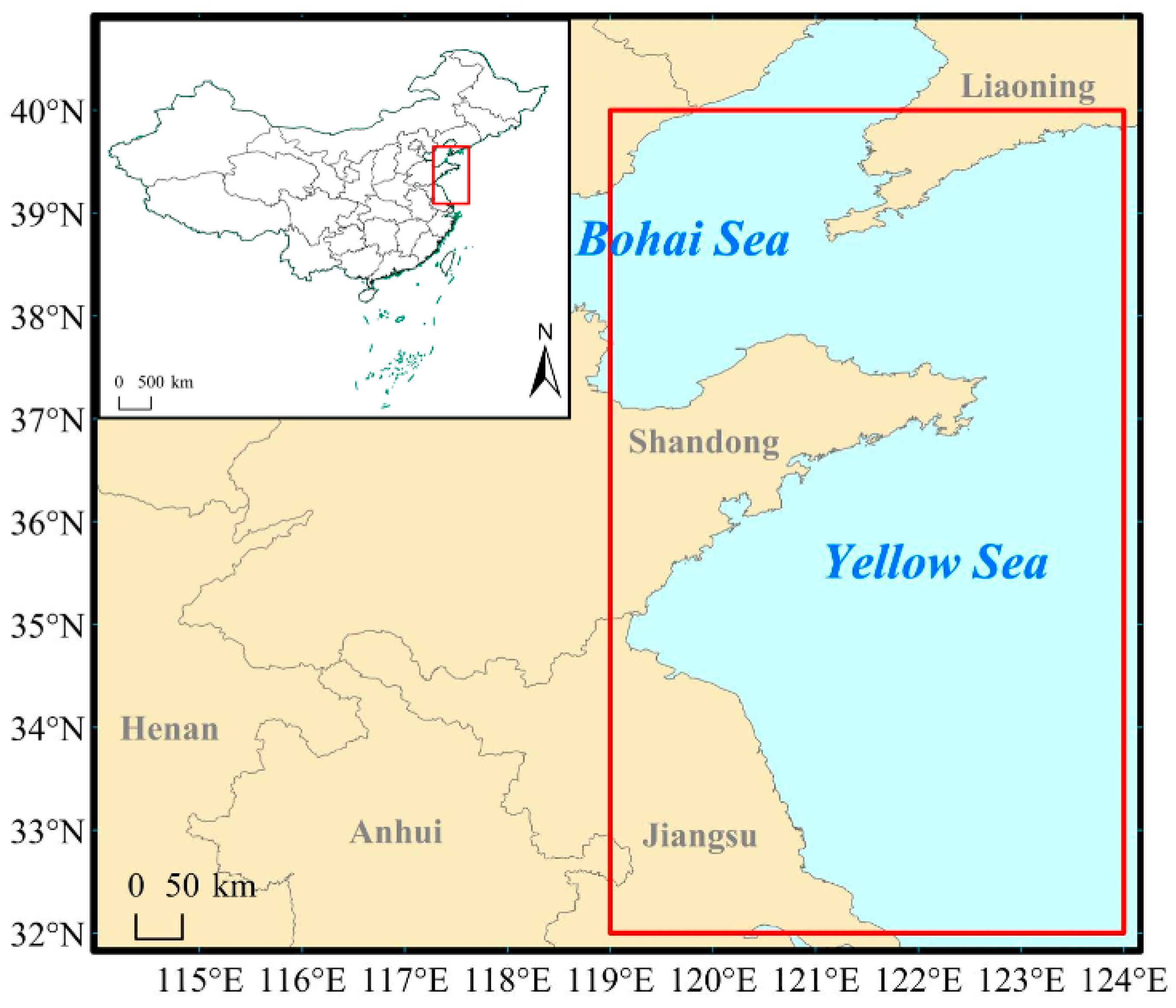
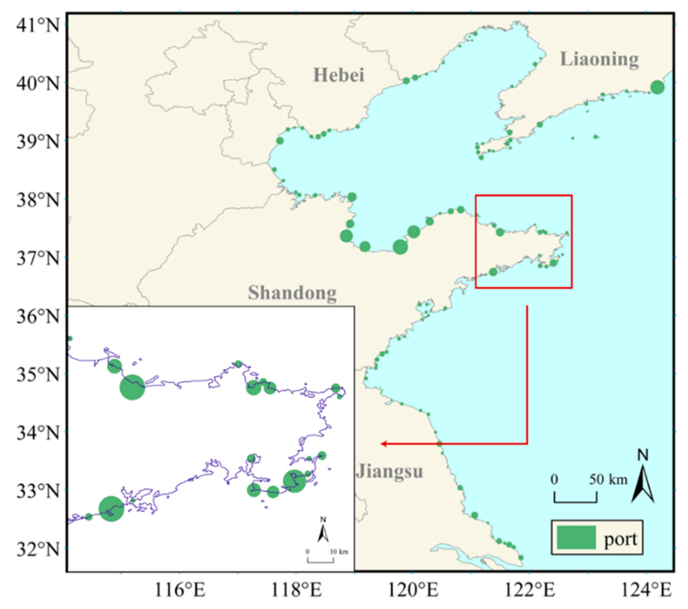
2.1. Study Area

The study sea in this article consists of the largest continental sea in China, the Bohai Sea, and the semi-enclosed marginal sea of the Western Pacific, the Yellow Sea, with a total area of approximately 477,000 km² [60,61] (Figure 1). The Bohai Sea and the Yellow Sea are the main sea areas for mariculture and marine fishing in the Liaoning, Hebei, Shandong, and Jiangsu Provinces of China.

Since the 1970s, the demand for seafood has raised the fishing intensity in the Bohai Sea and the Yellow Sea. Such a fishing intensity has exceeded the available fishery resources, prompting the government decision to implement a series of fishery policies aimed to achieve the sustainable utilization of resources [62]. To study the effect of fishing, the research area was selected based on the operating habits of Chinese trawlers. Specifically, the study area encompasses the geographic coordinates of ${119}^{°} \mathrm{E}~{124}^{°} \mathrm{E}$, ${32}^{°} \mathrm{N}~{40}^{°} \mathrm{N}$, as depicted in Figure 1.

2.2. Data Pre-Processing and Labeling

The satellite data were provided by the National Fishing Vessel Dynamic Monitoring and Management System, including the vessel position messages of trawlers from Liaoning, Hebei, Shandong, and Jiangsu Provinces along the coasts of the Bohai Sea and the Yellow Sea. The data spanned from 0:00 on 1 September 2019 to 24:00 on 31 December 2021, with a total collection of 4917 trawlers, and from 0:00 on 1 January 2022 to 24:00 on 30 April 2023, with a total collection of 4680 trawlers.

The satellite data included a series of position messages for each vessel, consisting of the vessel name, MMSI code (Fishing Vessel Maritime Mobile Communication Service Identification Code), location, timespan, instantaneous speed, and instantaneous course. According to the range limitation, data that were incomplete or transfinite in longitude, latitude, speed, and time were removed for each position message. The distance between each location and the Chinese coastline was calculated. The new “segment” was divided according to the time of entry and exit from the port. The distance and time between consecutive points were calculated, and if these implied an unrealistic speed between locations, or if the time between two points was greater than 3 h due to the impact of signal fluctuations during satellite data transmission and reception, the segment was divided. Segments with fewer than 5 position points were eliminated.

This study selected 32 trawlers randomly, encompassing 788,908 vessel position data points between September 2019 and December 2021. The vessel location data were labeled according to the segments, and a departure route map was created by plotting the vessel location and speed data for each segment, ordering by time using geographic information system software Arcmap 10.8 (ESRI, Redlands, CA, USA). Multiple researchers analyzed the fishing behavior by integrating prior knowledge, such as fishery information and the characteristics of trawling operations recorded in the literature, expert experience, fishermen surveys, and fishing logs. The start and end times of the trawling operations were determined and recorded, and the vessel location data during the fishing behavior were marked as “1”, or “0” otherwise. The labeling process was conducted using a multi-person, cross-review approach to ensure objective and precise annotations.

2.3. Feature Extraction

To efficiently recognize fishing behavior using machine-learning algorithms, this paper extracted 11-dimensional features from each position data, forming feature vectors. Firstly, 10-million-coastline data were downloaded from Natural Earth (https://www.naturalearthdata.com/downloads/10m-physical-vectors/10m-coastline/, accessed on 3 November 2021), and the shortest distance between the vessel location and coastline was calculated for each data entry. Based on the docking information of fishing vessels and high-resolution remote-sensing maps, the researchers manually labeled the ports along the coasts of the Bohai Sea and the Yellow Sea in China, as shown in Figure 2, and calculated the distance between each vessel location and the nearest port. Furthermore, the time difference between the preceding and subsequent position data points, the actual distance, theoretical average speed, difference in azimuth, and the rate of change in azimuth were calculated. This study also recorded real-time speed, local time, and month.

2.4. Fishing Behavior Recognition Based on the Slime Mould Algorithm-Optimized Light Gradient-Boosting Machine Algorithm

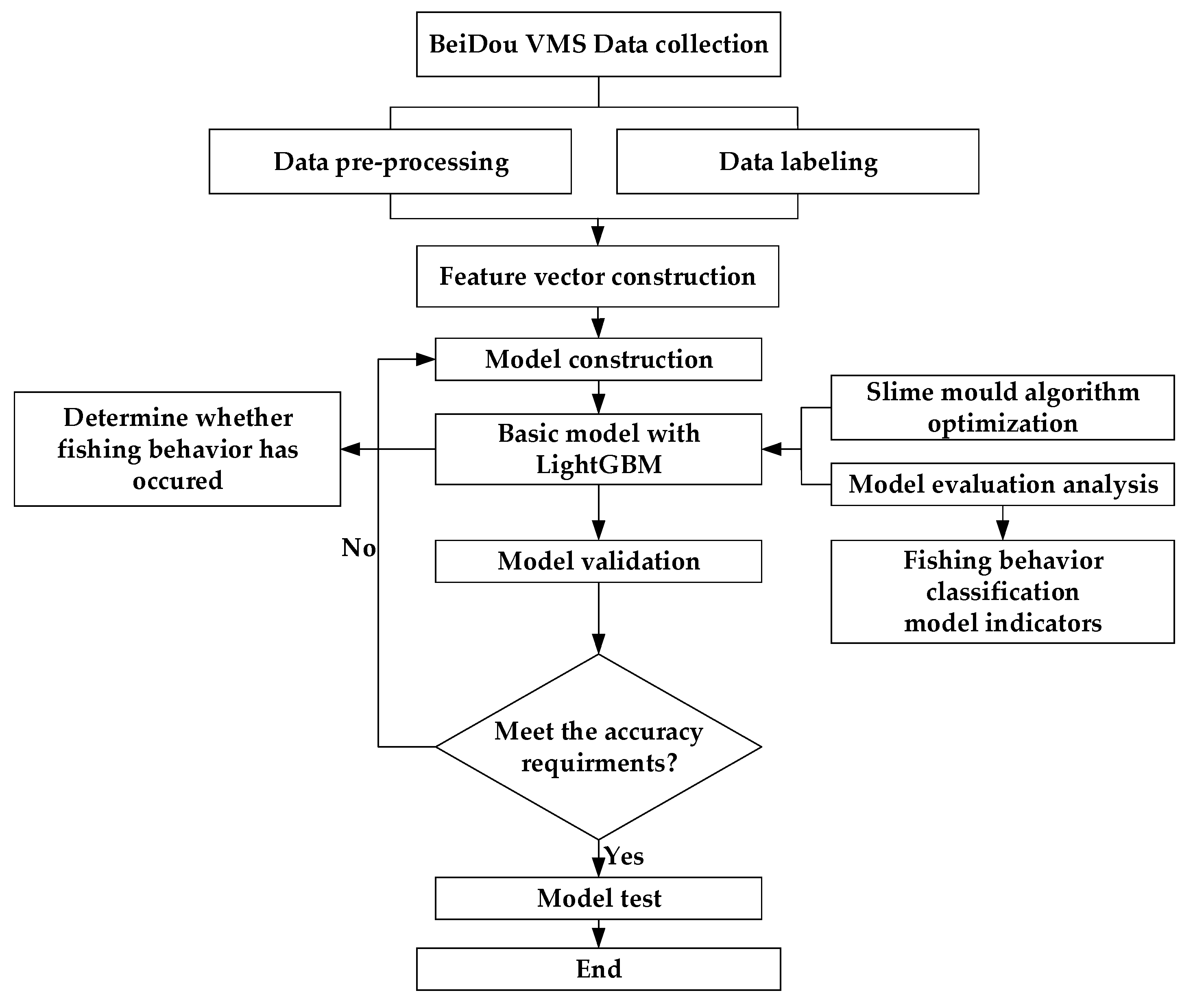
2.4.1. An Overview of the Fishing Behavior Recognition Model

Based on Beidou vessel-monitoring system data, the feature vectors were constructed through feature engineering. The optimized LightGBM algorithm, enhanced through the use of SMA, was employed to determine whether trawlers were engaged in fishing activities. The specific workflow of the algorithm is depicted in Figure 3.

During the training process, the hyperparameters of the LightGBM were optimized by the SMA algorithm based on the fitness function results until the optimal parameters were found. The entire algorithm was mainly divided into five steps: (1) data collection; (2) cleaning and labeling; (3) feature vector extraction; (4) model training with LightGBM optimized by SMA; (5) model evaluation with the dataset.

2.4.2. Principle of SMA-LightGBM

This study aimed to overcome the limitations of previous models by building an SMA-optimized smart model that is able to recognize the fishing behavior of trawlers quickly and more accurately.

• LightGBM Algorithm

LightGBM [63], a high-performance gradient-boosting framework, was chosen as the classifier for recognizing fishing behavior. Based on the decision tree algorithm, it adopted the histogram algorithm to accelerate the training process and performed data processing based on gradient-based one-side sampling and exclusive feature bundling to improve computational efficiency. The decision tree growth strategy of layer-wise growth was discarded in favor of a leaf-wise growth strategy with depth constraints, ensuring efficiency while mitigating overfitting.

Histogram algorithm: Specifically, LightGBM addressed the issues of substantial memory consumption and low-efficiency encountered by XGBoost when handling large-scale high-dimensional data by replacing the traditional pre-sorting algorithm with the histogram algorithm. LightGBM converted continuous floating-point data into bin data. During the data traversal process, it calculated the cumulative values for each discrete value within the histogram and determined the optimal splitting points based on the distribution of these discrete values.

Gradient-based one-side sampling: Moreover, gradient-based one-side sampling (GOSS) was proposed to achieve a balance between reducing the number of data instances and ensuring accuracy [63]. To be specific, an instance is represented as an N-dimensional vector $x_i$. The information gain to split the node with the most gain can be formulated as:

$$\begin{gathered} V_{j|D}\left(k\right)=\frac{1}{n_D}\left(\frac{{\left({{\displaystyle \sum }}_{\left\{x_i\in D:x_i\le k\right\}}{g}_i\right)}^2}{n_{l|D}^j\left(k\right)}+\frac{{\left({{\displaystyle \sum }}_{\left\{x_i\in D:x_i>k\right\}}{g}_i\right)}^2}{n_{\gamma |D}^j\left(k\right)}\right) \\ {n}_{l|D}^j\left(k\right)={\displaystyle \sum }I\left[x_i:x_i\in D, x_i\le k\right] ; n_{\gamma |D}^j\left(k\right)={\displaystyle \sum }I\left[x_i:x_i\in D, x_i>k\right] \end{gathered}$$

(1)

where $V_{j|D}\left(k\right)$ is the information gain of feature $j$ at position $k$, $D$ denotes the training set on a node, and $g_i$ represents the gradient of the loss function, for instance, $i$.

The training instances were made similar according to the absolute values of their gradients in descending order. The top a% instances with the larger gradients were kept as the instance subset A was obtained [64]. Then, randomly selected b% instances from the remaining subset B were obtained. Finally, when calculating the information gain, GOSS multiplied the sampled data with a low gradient via the weight (100 − a)/b [64]. Thus, the instances were split according to the estimated variance gain over subsets A and B:

$$\widetilde{V_j}\left(k\right)=\frac{1}{n_D}\left(\frac{{\left({{\displaystyle \sum }}_{\left\{x_i\in A_l\right\}}{g}_i+\frac{1-a}{b}{{\displaystyle \sum }}_{\left\{x_i\in B_l\right\}}{g}_i\right)}^2}{n_{l|D}^j\left(k\right)}+\frac{{\left({{\displaystyle \sum }}_{\left\{x_i\in A_{\gamma }\right\}}{g}_i+\frac{1-a}{b}{{\displaystyle \sum }}_{\left\{x_i\in B_{\gamma }\right\}}{g}_i\right)}^2}{n_{\gamma |D}^j\left(k\right)}\right)$$

(2)

Exclusive feature bundling: LightGBM also conducted feature dimension sampling, further enhancing the speed of model training. The exclusive feature bundling algorithm (EFB) bound mutually exclusive features together, reducing dimensionality. EFB addressed a non-deterministic polynomial hard problem, meaning that it allowed a small number of data points between features to be non-exclusive, decreasing the occurrence of conflicting results in fewer feature bundles, thereby further improving computational efficiency.

The objective function $Obj$ could be formulated as:

$$\begin{gathered} Obj={\displaystyle \sum }_{m=1}^M\left[G_{tm}{\omega }_{tm}+\frac{1}{2}\left(H_{tm}+\lambda \right){\omega }_{tm}^2\right]+\mathsf{\gamma }\mathrm{M} \\ {G}_{tm}={{\displaystyle \sum }}_{i\in I_{tm}}{g}_i; H_{tm}={{\displaystyle \sum }}_{i\in I_{tm}}{h}_i \end{gathered}$$

(3)

where m represents the m-th leaf node, M represents the maximum total number of leaves, $I_{tm}$ represents leaf nodes, and ${\omega }_{tm}$ is the best value for the decision of the tree’s mth leaf node. $G_{tm}$ is the first derivative of Taylor expansion, $H_{tm}$ represents the second-order derivative in the Taylor expansion, and γ and λ are the hyperparameters for regularization.

It was evident that the LightGBM algorithm involved a multitude of hyperparameters, making network optimization challenging. This study employed metaheuristic intelligent algorithms to optimize LightGBM.

2.

Slime Mould Algorithm

The Slime Mould Algorithm is a novel metaheuristic algorithm that effectively emulates the propagation and foraging behavior inherent of a slime mould. This algorithm uses adaptive weights to simulate the process of producing positive and negative feedback of the propagation wave of a slime mould based on bio-oscillators to form the optimal path to connect food with an excellent exploratory ability and exploitation propensity [65], thereby rendering SMA a highly effective parameter optimization algorithm.

Approach food: Slime mould moves based on the odor in the air. The approaching behavior could be mathematically expressed as the following formulae:

$$\begin{gathered} X_{i,j}\left(t+1\right)=\{\begin{array}{c}{X}_{b,j}\left(t\right)+v_b·\left(W·X_{A,j}\left(t\right)-X_{B,j}\left(t\right)\right), r<p\\ v_c·X_{i,j}\left(t\right) , r\ge p\end{array} \\ p=\tanh \left|S\left(i\right)-D_F\right|, I=1,2,\cdots ,N. \\ a=\mathrm{arctanh}\left(-\left(\frac{t}{ma{x}_t}\right)+1\right) \end{gathered}$$

(4)

where $t$ denotes the current iteration, $v_b$ is a parameter with a range of [$-a, a$], $v_c$ linearly decreases from one to zero, $X$ represents the location of the slime mould, $X_{b,j}$ signifies the present location characterized by the highest concentration of food odor detected in the $j$-th dimension, $X_{A,j}$ and $X_{B,j}$ indicate two randomly chosen individual slime mould positions in the $j$-th dimensiton, $r$ represents a random number ranging from zero to one, $N$ signifies the size of the slime mould population, $S\left(i\right)$ denotes the fitness value of the $i$-th slime mould, $D_F$ represents the fitness value of the globally optimal smile mould, and $W$ represents the weight of the slime mould. The formula of $W$ is listed as follows:

$$\begin{gathered} W\left(SmellIndex\left(i\right)\right)=\{\begin{array}{c}1+r·log\left(\frac{bF-S\left(i\right)}{bF-wF}+1\right), 1\le i\le \frac{N}{2}\\ 1-r·log\left(\frac{bF-S\left(i\right)}{bF-wF}+1\right), \frac{N}{2}\le i\le N\end{array} \\ SmellIndex=sort\left(S\right) \end{gathered}$$

(5)

where $bF$ denotes the optimal fitness obtained in the current iterative process, $wF$ denotes the worst fitness value obtained in the iterative process currently, and $SmellIndex$ represents the sequence of the sorted fitness values (ascends in the minimum value problem).

Wrap food: When the veins approached food sources, the signals emitted within the slime mould stimulated internal biological oscillators, generating propagating waves that promoted cytoplasmic flow within the veins. Higher food concentrations resulted in stronger wave signals, faster cytoplasmic flow, and thicker veins; conversely, lower food concentrations led to thinner veins. The mathematical formula for updating slime mould positions is as follows:

$$X_{i,j}\left(t+1\right)=\{\begin{array}{c}{r}_1·\left(ub-lb\right)+lb, r_1<z\\ X_{b,j}\left(t\right)+v_b·\left(W·X_{A,j}\left(t\right)-X_{B,j}\left(t\right)\right), r_2<p\\ v_c·X_{i,j}\left(t\right) , r_2\ge p\end{array}$$

(6)

where $ub$ and $lb$ denote the upper and lower boundaries of the search range, $r_1$ and $r_2$ denote the random value in [0, 1], and $z$ was utilized to modulate the global and local search of the algorithm.

Oscillation: The value of $v_b$ oscillated randomly between [$-a, a$] and gradually approached zero as the iterations increased. The value of $v_c$ oscillated between [$-b, b$] and tended to zero eventually.

$$\begin{gathered} a=\mathrm{arctanh}\left(-\left(\frac{t}{ma{x}_t}\right)+1\right) \\ b=-\left(\frac{t}{ma{x}_t}\right)+1 \end{gathered}$$

(7)

where $t$ denotes the current iteration.

3.

The Slime Mould Algorithm-Optimized LightGBM

This study aims to employ LightGBM to classify the fishing behavior of trawlers. However, multiple parameters need to be adjusted to use LightGBM, and the choice of parameter values significantly impacts the performance of LightGBM, meaning that grid search and manual tuning need to take place, which are time-consuming and labor-intensive. Therefore, this article proposed the use of SMA to optimize LightGBM. The process of optimizing the parameters of LightGBM using the SMA algorithm is as follows:

Step 1: Determine the number and ranges of parameters to be optimized. The parameters to be optimized in LightGBM include the number of leaf nodes in each decision tree, tree depth, minimum leaf node instance weight, regularization parameters γ and λ, instance and feature sampling rates, learning rate, and the number of iterations. Set the upper and lower bound arrays ‘$ub$’ and ‘$lb$’ for each parameter based on their value ranges.

Step 2: Utilize the average accuracy of the cross-validation of the LightGBM model as the fitness function for SMA.

Step 3: Initialize the population of the slime mould and calculate the fitness of all the slime mould positions.

Step 4: Determine whether the maximum iteration count has been attained. If the current iteration count exceeds the maximum, proceed to Step 5. Otherwise, update the slime mould positions and continue the optimization process based on Formulas (4)–(7).

Step 5: Output the parameter optimization results.

Following the aforementioned steps, the trawler fishing behavior recognition model based on SMA-LightGBM is obtained. The pseudo-code of SMA-LightGBM is depicted as shown in Algorithm 1.

Algorithm 1 Pseudo-code of SMA-LightGBM

Inputs: The population size $N$ and maximum number of iterations $ma{x}_t$ The upper and lower boundaries of the nine parameters of LightGBM  Outputs: The best solution Initialize the positions of slime mould $X_i$ ($i=1,2,\cdots ,n$) while iteration $t \le$ $ma{x}_t$ do Calculate the cross-validation score of LightGBM as fitness Update $bF$, $X_b$ Calculate the $W$ by Equation (5)   for each search portion $X_i$ do    Update $p$, $v_b$, $v_c$ Update positions by Equation (6) Return $bF$ and $X_b$

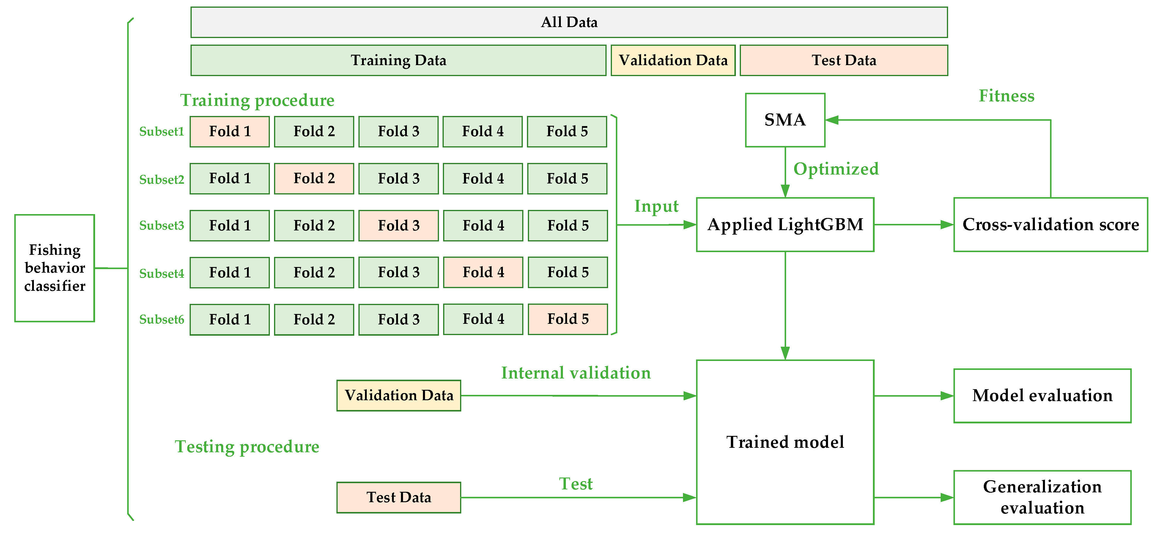
2.4.3. Training and Testing Phases of the Fishing Behavior Classifier

A total of 788,908 vessel position data points were annotated in the experiment, covering 32 trawlers from September 2019 to December 2021. Following data preprocessing and feature vector extraction, 675,571 feature vectors were generated. During the training and testing process of the fishing behavior classifier, one-third of the entire dataset, which included the vessel position data of 11 trawlers, was reserved for tests to evaluate the generalization ability of the trawler fishing behavior classifier model. The remaining data, which included the vessel position data of 21 trawlers, were evenly split into five parts. Of these, one-fifth served as a validation set for validation during the model tuning process, and the other four-fifths were used for five-fold cross-validation. This resulted in a final training set of 353,083 feature vectors, a validation set of 88,269 feature vectors, and a testing set of 234,218 feature vectors.

The training and testing procedure of the fishing behavior classifier is shown in Figure 4. The experiment process is outlined as follows.

Step 1: The training dataset containing 353,083 vectors is randomly split into 5 subsets, with one subset serving as the training validation set, which is then input into the lightGBM model.

Step 2: Initialize the SMA parameters, set the number of optimization parameters, and configure the category parameters.

Step 3: Start training with fold 2–fold 5 of subset 1 and observe the change in the accuracy of the LightGBM optimized by SMA.

Step 4: Reset the parameters, such as population size $N$ and the maximum number of iterations $ma{x}_t$.

Step 5: Evaluate the fishing behavior classifier using fold 1.

Step 6: Repeat Step 4–Step 5 until the desired precision is achieved.

Step 7: Update the train set to subset 2 and the validation set to fold 2. Repeat Step 2–Step 6 five times until the five-fold cross-validation is finished, and an average accuracy is obtained. Extract the model hyperparameters with the highest average accuracy.

Step 8: Test the model with the best parameters using the validation set to evaluate metrics for the classification ability of the fishing behavior classifier.

Step 9: Test the model with the best parameters using the test set to determine accuracy, sensitivity, specificity, and the Matthews correlation coefficient as evaluation metrics for the generalization ability of the fishing behavior classifier.

This experiment implemented Extreme Learning Machine (ELM), Random Forest (RF), eXtreme Gradient Boosting (XGBoost), and Light Gradient-Boosting Machine (LightGBM). Additionally, LightGBM was optimized using the following algorithms separately: a Genetic Algorithm (GA), Harris Hawks Optimization (HHO), and a Slime Mould Algorithm (SMA). ELM was implemented using Matlab (R2021a) (MathWorks, Natick, MA, USA), and the remaining models were implemented in the Python programming language. In the feature generation process, to calculate the distance from the trawler positions to the coastline and ports, the R programming language was utilized within RStudio. The experimental hardware platform comprised an Intel Core i9-11900K CPU (Intel Corporation, Santa Clara, CA, USA) with a 3.5 GHz base clock frequency and 128 GB of RAM.

The ranges of 9 parameters were set according to the attributes of LightGBM. The range of ‘Number of iterations’ was defined to be within [1, 500], the range of ‘learning rate’ was defined to be within [0.00001, 1], the range of ‘max depth’ was set to be within [2, 1000], and the range of ‘Minimum leaf node instance weight’ was set to be within [1, 1000]. The ranges of ‘Regularization parameters γ’, ‘Regularization parameters λ’, ‘Instance sampling rate’, and ‘Feature sampling rates’ were set to be within [0.001, 1], and the range of ‘Number of leaf nodes’ was defined to be within [2, 1000].

2.4.4. Performance Evaluation of the Fishing Behavior Classifier

To evaluate the performance of the classifier of trawler fishing behavior, four metrics [66,67] were utilized: specificity (SP), sensitivity (SN), accuracy (ACC), and the Matthews correlation coefficient (MCC), which are defined as follows:

$$\begin{gathered} Specificity\left(SP\right)=\frac{TN}{TN+FP} \\ Sensitivity\left(SN\right)=\frac{TP}{TP+FN} \\ Accuracy\left(ACC\right)=\frac{TP+TN}{TP+FP+TN+FN} \\ Matthews correlation coefficient\left(MCC\right)=\frac{TP\times TN-FP\times FN}{\sqrt{\left(TP+FN\right)\left(TP+FP\right)\left(TN+FP\right)\left(TN+FN\right)}} \end{gathered}$$

(8)

where $TP$ (true positive) represents the number of positive samples correctly recognized as fishing status; $TN$ (true negative) represents the number of negative samples correctly identified as non-fishing status; $FP$ (false positive) represents the number of negative samples incorrectly identified as fishing status when the real status was non-fishing; and $FN$ (false negative) represents the number of positive samples incorrectly identified as non-fishing status when the real status was fishing.

2.5. Calculation Method of the Fishing Effort

According to the calculation method of the Food and Agriculture Organization of the United Nations, fishing effort should be expressed in terms of engine power and fishing operation days (kW·d) [68,69]. In this study, the calculation method for fishing effort referred to papers [57,68], with time measured in hours, and fishing effort was quantified in kW·h. When trawler $i$ was engaged in fishing activities, assuming that the study area could be divided into $S$ grids, the formula for calculating fishing effort within the study grid was as follows:

$$E={\displaystyle \sum }_{s=0}^S{\displaystyle \sum }_{i=0}^I{\displaystyle \sum }_{n=0}^N\left(T_{i,m}-T_{i,m-1}\right)\times W_i\times P_{i,m}$$

(9)

where $m$ represents a position in a grid for a specific trawler, $T_{i,m}$ and $T_{i,m-1}$ denote the time at consecutive points along the trajectory of trawler $i$, $W_i$ denotes the engine power of the trawler $i$, $P_{i,m}$ represents the operational status of trawler $i$ at position $m$ at $T_{i,m}$, $N$ indicates the number of positions for trawler $i$ in the specific grid, $I$ represents the number of trawlers in the $s$-th grid, $S$ denotes the number of grids, and $E$ signifies the total fishing effort within the study area.

This study analyzed the position data of 4969 trawlers from 2019 to 2021, as well as 4680 trawlers from 2022 to 2023. The SMA-LightGBM algorithm was utilized for the purpose of recognizing fishing behavior and duration. The fishing effort was calculated and evaluated.

3. Results

3.1. Experiment and Evaluation of Fishing Behavior Recognition

During the training process of the SMA-LightGBM classifier, and based on the results of multiple experiments, the SMA algorithm parameters were configured with a ‘population size N’ of 200 and ‘Epoch’ of 20. Upon configuring the parameters, SMA-LightGBM proceeded to train the dataset following the algorithm detailed in Section 2.4.3. Upon completion of the training process, it provided the optimal parameter combination. The optimal parameters, as presented in this study, are outlined in

Table 1. Parameters of LightGBM optimized by SMA.

Parameter	Value	Parameter	Value	Parameter	Value
Number of iterations	394	Learning rate	0.2393	Max depth	97
Minimum leaf node instance weight	82.0298	Regularization parameters γ	0.5233	Regularization parameters λ	0.3453
Instance sampling rate	0.2869	Feature sampling rate	0.8381	Number of leaf nodes	353

.

After determining the optimal parameters, model testing was conducted. The final test results are presented in

Table 2. Comparison of the precision rate of machine-learning classifiers.

Methods	Test Result
	ACC	MCC	SN	SP
ELM	0.9417	0.8844	0.9187	0.9652
RF	0.9821	0.9643	0.9925	0.9723
XGBoost	0.9820	0.9640	0.9892	0.9752
LightGBM	0.9811	0.9622	0.9860	0.9766
GA-LightGBM	0.9809	0.9619	0.9859	0.9763
HHO-LightGBM	0.9819	0.9638	0.9879	0.9763
SMA-LightGBM	0.9823	0.9646	0.9875	0.9775

.

This study initiated a comparative analysis of the experimental results among ELM, RF, XGBoost, and LightGBM. The outcomes, as assessed through metrics, clearly indicated that LightGBM trained with empirical parameters excelled in fitting the trawler fishing behavior. It outperformed other algorithms in terms of ACC and MCC. This confirmed that in contrast to ELM, ensemble learning algorithms like RF, XGBoost, and LightGBM exhibited superior suitability for fitting trawler fishing behavior data. Furthermore, compared to the bagging parallel mechanism of RF, the boosting mechanisms of XGBoost and LightGBM were better tailored to the trawler fishing behavior recognition task. When juxtaposed with XGBoost, LightGBM showed notable advantages, including swifter execution, more efficient memory usage, and heightened aptitude for handling extensive trawler feature data without compromising accuracy. However, an interesting observation during the test revealed slightly diminished ACC and MCC for LightGBM. This discrepancy could be attributed to the manual parameter selection process. As a result, metaheuristic algorithms such as GA, HHO, and SMA were implemented to enhance the optimization of parameter selection in the LightGBM model.

To further optimize the fishing behavior recognition model, this study applied various metaheuristic algorithms to fine-tune the hyperparameters of LightGBM. Table 2 presents the results after optimization using GA, HHO, and SMA. It is evident that LightGBM optimized by SMA performed significantly better on the test sets. In comparison to empirical parameter tuning, SMA-LightGBM exhibited a noteworthy enhancement. On the test dataset, the model demonstrated a pronounced improvement, with an increase of 0.12 percentage points in accuracy and 0.0024 in MCC. To be more specific, compared to empirical tuning, SMA-LightGBM correctly identified an additional 271 samples on the test set, thereby securing the highest recognition performance in this experiment.

As the outcomes of this experiment are to be subsequently employed to evaluate the fishing effort of trawlers, the primary focus should be on the accuracy and Matthews Correlation coefficient during the external testing phase. For the estimation of the fishing behavior of all trawlers from 2019 to 2023, we would exclusively utilize the SMA-LightGBM model.

3.2. Estimating Spatiotemporal Fishing Effort of Trawlers

The fishing effort was quantified for the time duration from September 2019 to April 2023, as presented in Figure 5.

Based on the analysis from the figure, it can be observed that most fishing effort was concentrated in three specific areas: ① The first area encompassed 121° E~124° E, 35.5° N~39° N, covering an estimated 26.25% of the total grid area. Trawlers within this region focused their efforts on searching for fish schools, allocating approximately 55.3% of their total fishing time over a span of five years. This area stood out for its abundant fish resources. ② The second focal area spanned 119.7° E~122.7° E, 33.8° N~35.5° N, accounting for roughly 12.75% of overall grid coverage. It ranked as the second-largest fishing hotspot, with an investment of approximately 18.75% of total fishing time. ③ The third region covered 123° E~124° E, 33.5° N~35° N, contributing to about 3.75% of the total grid area. Trawlers were active in this area, seeking fish schools and spending around 6.14% of their total fishing effort there despite its relatively smaller geographical extension. These insights highlighted the distribution of fishing effort within these regions and their significance in the study area.

The spatial distribution of fishing hotspots throughout the year, denoted by Figure 5C–E and corresponding to the years 2020, 2021, and 2022, respectively, was consistent with the previously outlined characteristics. However, Figure 5B,F, representing the second half of 2019 and the first half of 2023, respectively, displays some deviations in the distribution of hotspot areas compared to the overall annual patterns. This observation indicated that the distribution of fishing hotspots may exhibit temporal variations. Consequently, this study conducted a month-by-month analysis to investigate the relationship between fishing effort and geographical coordinates, as depicted in Figure 6.

Figure 6 illustrates the temporal dynamics of the fishing effort from September 2019 to April 2023, encompassing a total of 44 months. The graph illustrates a remarkable periodic variation in the distribution of fishing effort concerning both time and coordinates. Specifically, there was a gradual concentration of fishing effort hotspots toward higher latitudinal and longitudinal coordinates during the period from September to January each year. In the subsequent months, particularly in January and February, there was a notable reduction in trawling activities, with the period from March to April witnessing an upward trajectory in fishing effort across various latitude and longitude regions. The months of May to August exhibited minimal trawling operations, with few exceptions for permitted trawlers. Notably, the fishing effort of trawlers exhibited a significant relationship with time. The distribution of fishing effort by latitude showed a positive slope of approximately 2 concerning time, and the distribution by longitude demonstrated a negative slope of approximately −1.25, as indicated by the red dashed line in Figure 6.

Actually, this phenomenon could be reasonably explained by human activities. To provide a more lucid illustration of the correlation between trawling activities and human actions, a line chart depicting the temporal fluctuation in fishing duration across months was generated, as shown in Figure 7.

The fishing closed season of the Bohai Sea and the Yellow Sea lasts from May to August, and the Lunar New Year falls around January to February every year. During these two intervals in this study, fishermen tended to reduce their fishing activities. Therefore, the most active trawling period occurred from September to December and from March to April. Specifically, in September, most trawlers headed out to sea, with fishing activity being concentrated near the coastline. As the Lunar New Year approached, some trawlers returned to celebrate the Chinese New Year. Additionally, a portion of the fishing fleet ventured further into the deeper sea to carry out fishing operations. This corresponded to the periodic characteristics of fishing times shown in Figure 7 and explained the distribution of fishing effort from September to October 2019 and January to April 2023, as depicted in Figure 5.

Indeed, from Figure 7, it is evident that from September 2019 to August 2021, the fishing operation duration was relatively low, but it started to recover from September 2021. This can be attributed to restrictions related to the COVID-19 pandemic. As the pandemic became less severe, fishermen’s fishing activities increased. Presently, fishermen have fully resumed their normal fishing operations.

4. Discussion

4.1. Model and Fishing Effort Estimation

This article proposed an SMA-LightGBM algorithm to construct a fishing behavior recognition model for trawlers, achieving remarkable performance on the test set. However, it still holds a certain degree of uncertainty, stemming from various sources, including data uncertainties, model complexity uncertainties, and uncertainties related to feature selection and scaling. The raw data used in the study were derived from a satellite. Although the data were corrected multiple times before entering the system, exceeding the limit was still inevitable. To address these issues, data cleaning was performed before training, but it may not have entirely eliminated the impact of data noise on the model. Thus, five-fold cross-validation was utilized to select optimal hyperparameters, minimizing the impact of data noise on model performance. Moreover, the introduction of the histogram algorithm in LightGBM simplified data representation and provided a regularization effect, preventing overfitting during the training phase and enhancing generalization performance. To address the uncertainties regarding model complexity, the loss function of LightGBM retained the L1 and L2 regularization terms from XGBoost, controlling the complexity of the model and improving generalization performance. Concerning uncertainties in feature selection and scaling, this study adopted features and scaling methods used by [61]. Supplementary adjustments based on the characteristics of the Chinese trawlers were made, such as incorporating harbor and anchorage locations along the coast of the Bohai Sea and the Yellow Sea and introducing features like acceleration and azimuth change rates. From the performance of the experiments, the selected features in this study effectively captured the characteristics of trawling behavior, providing valuable information for model training.

To evaluate the calculation error of fishing effort, a dataset was compiled of trawlers with varying power capacities. Within this dataset, trawlers with power below 100 kW exhibited a mean absolute error (MAE) of 0.0392 kW·h and a coefficient of determination ($R^2$) score of 0.9885. Trawlers featuring power ranging from 100 kW to 300 kW exhibited a MAE of 0.2155 kW·h and an $R^2$ score of 0.9771. The remaining trawlers possessed power exceeding 300 kW. For this group, the MAE was 0.5976 kW·h, and the $R^2$ score stood at 0.9747. The complete dataset produced a MAE of 0.3031 kW·h and an $R^2$ score of 0.9772. These results underscored the significant influence of vessel power on the accuracy of the fishing effort estimation, indicating a higher degree of accuracy in assessments for lower-powered trawlers and a more pronounced impact on higher-powered vessels.

In practice, the prediction of this study may exhibit a tendency to overestimate actual fishing effort. Regarding the determination of fishing time, both the internal and external assessments of the SMA-LightGBM algorithm revealed that the fishing behavior recognition model demonstrated higher sensitivity but lower specificity. In the external test set, comprising 112,687 positive samples and 121,531 negative samples, the predictions generated by the SMA-LightGBM algorithm resulted in 114,025 positive samples and 120,193 negative samples. This indicated that the algorithm exhibited a heightened rate of FP, signifying the propensity to incorrectly classify non-fishing conditions as fishing status. This may be the underlying cause for the elevated predicted values observed in this study. Additionally, in the context of trawler power, this study utilized rated engine power for calculating fishing effort. It should be noted that for vessels operating at lower speeds, this approach might contribute to an overestimation of the effort.

To further improve the precision of fishing effort assessment and reduce estimation errors, this study suggests the use of three optimization strategies: ① Feature enhancement: Augment model accuracy by extracting spatial information between vessels as feature parameters. ② Algorithm enhancement: Explore the implementation of deep-learning architectures, such as Transformer, to construct models for the recognition of trawling fishing behaviors, thereby elevating model efficiency. ③ Data augmentation: Expand the dataset to enhance model performance. Given the labor-intensive nature of ship position data labeling, increasing the size of the dataset can be beneficial. Furthermore, optimizing the power calculation process by refining the method for estimating a trawler’s operational power can significantly improve the precision of fishing effort predictions.

4.2. Model Performance for Fisheries’ Management and Policy Implementation

The result of the fishing behavior recognition model for trawlers can be utilized to analyze the fishing operations associated with each positional piece of data and directly assist fisheries’ management, offering functionalities such as querying the fishing operational status of vessels, investigating fishing locations and durations, and assessing the progress of implementing fishing quotas for vessels. The model provides an intuitive reflection of fishing activities and footprints, offering accurate statistics of fishing operations to the minute level and contributing to furnishing fisheries’ management with accurate data support.

The result of the model could be utilized to estimate fishing effort, exhibiting a higher resolution compared to statistical yearbooks, providing a more detailed and intuitive representation of fishing intensity. As an input factor for fishing capacity, precise fishing effort data can be combined with output factors, providing a more accurate basis for the assessment of fishing capacity and productivity. This would offer an evaluative foundation for the effectiveness of fisheries’ management, promoting the conservation and sustainable development of fishery resources. The estimated fishing effort can be utilized in conjunction with biomass information [70] to formulate the resource management goals of fisheries, improve the fishing management system, and provide a basis for total allowable catch (TAC). A noteworthy example is Italy, where research has long been conducted to integrate the fishing effort and catch quantity of trawl fishing vessels as a basis for formulating management objectives in trawl fishing. This approach held significant importance in mitigating the adverse impacts of trawl fisheries on marine resources and biological communities [71]. Since the introduction of TAC in China in 2017, its application has been limited to a few pilot areas. The data calculated by this research may contribute to the scientific formulation of TAC and facilitate the establishment of a scientifically based fishery management system in China that integrates ecological assessments.

Meanwhile, this study provides assistance in three key areas for the implementation of policies: ① Assisting in fisheries’ law enforcement supervision: China has implemented strict management measures against fishing methods, such as trawling, that are harmful to fishery resources and the environment. China has already completely banned bottom trawlers from fishing operations in nearshore areas. The conclusions and computational models derived in this study can effectively guide Chinese fishery law enforcement agencies to concentrate on law enforcement and supervision in hotspot areas and periods, including imposing penalties and correcting the illegal fishing activities of trawlers, combating IUU (illegal, unreported, and unregulated) fishing, and maintaining the order of normal production operations. ② Facilitating the control of marine fishing input intensity: To effectively control marine fishing intensity, China has implemented long-term policy adjustments, regulating the total number and power of fishing vessels. According to statistics published by the Ministry of Agriculture and Rural Affairs of the People’s Republic of China, from 2015 to 2020, the country reduced the number of marine fishing vessels by 20,414 and total power by 10%. The proposed method for assessing fishing effort in this paper provided a more intuitive reflection of fishing input intensity. It has the ability to assist fishery management authorities in accurately understanding the spatiotemporal distribution of fishing input intensity in the Bohai Sea and the Yellow Sea. Additionally, this method allowed for a multidimensional analysis of the main contributors to fishing intensity to be conducted, considering factors such as fishing zones and the homeports of fishing vessels. This approach was beneficial for reducing the number of vessels in hotspot areas, encouraging fishermen to transition to other industries, and promoting the healthy and sustainable development of the fishing industry. ③ Promoting the implementation of quota-based fishing regulations: Major fishing nations worldwide have prioritized quota-based fishing regulations for key species as a pivotal measure to manage the output of fishery resources. The Bohai Sea, China’s sole semi-enclosed inland sea with distinct geographical advantages, is presently undergoing exploration for the implementation of quota-based fishing regulations by China’s fisheries’ management authorities, aiming to determine total fishing quotas and formulate allocation plans specific to the Bohai Sea. By integrating fishing effort data with catch data, this study enhanced the ability to reflect the abundance of fishing grounds. Regular data surveys contributed to a more accurate assessment of the resource output of fisheries and the production efficiency of fishing vessels. The outcomes of this research can serve as a foundational basis for shaping quota-based fishing policies, enabling fishery management authorities to methodically and judiciously determine total fishing quotas and allocate catch quotas for different regions and fishing vessels. This approach facilitated the achievement of the sustainable development and utilization of fishery resources.

5. Conclusions

This study proposed a novel algorithm, SMA-LightGBM, with which a fishing behavior recognition model for trawlers was developed. The fishing effort of over 4600 trawlers in the Bohai Sea and the Yellow Sea from September 2019 to April 2023 was calculated. The spatiotemporal distribution characteristics were estimated, and a comprehensive analysis was conducted. The conclusions we have drawn are as follows:

(1)

The presented method showed a remarkable generalization ability and high accuracy, sensitivity, specificity, and Matthews correlation coefficient in the test, with scores of 98.23%, 98.75%, 97.75%, and 0.9646, respectively. The MAE of the fishing effort of the trawlers was 0.3031 kW·h, and the R² score was 0.9772.

(2)

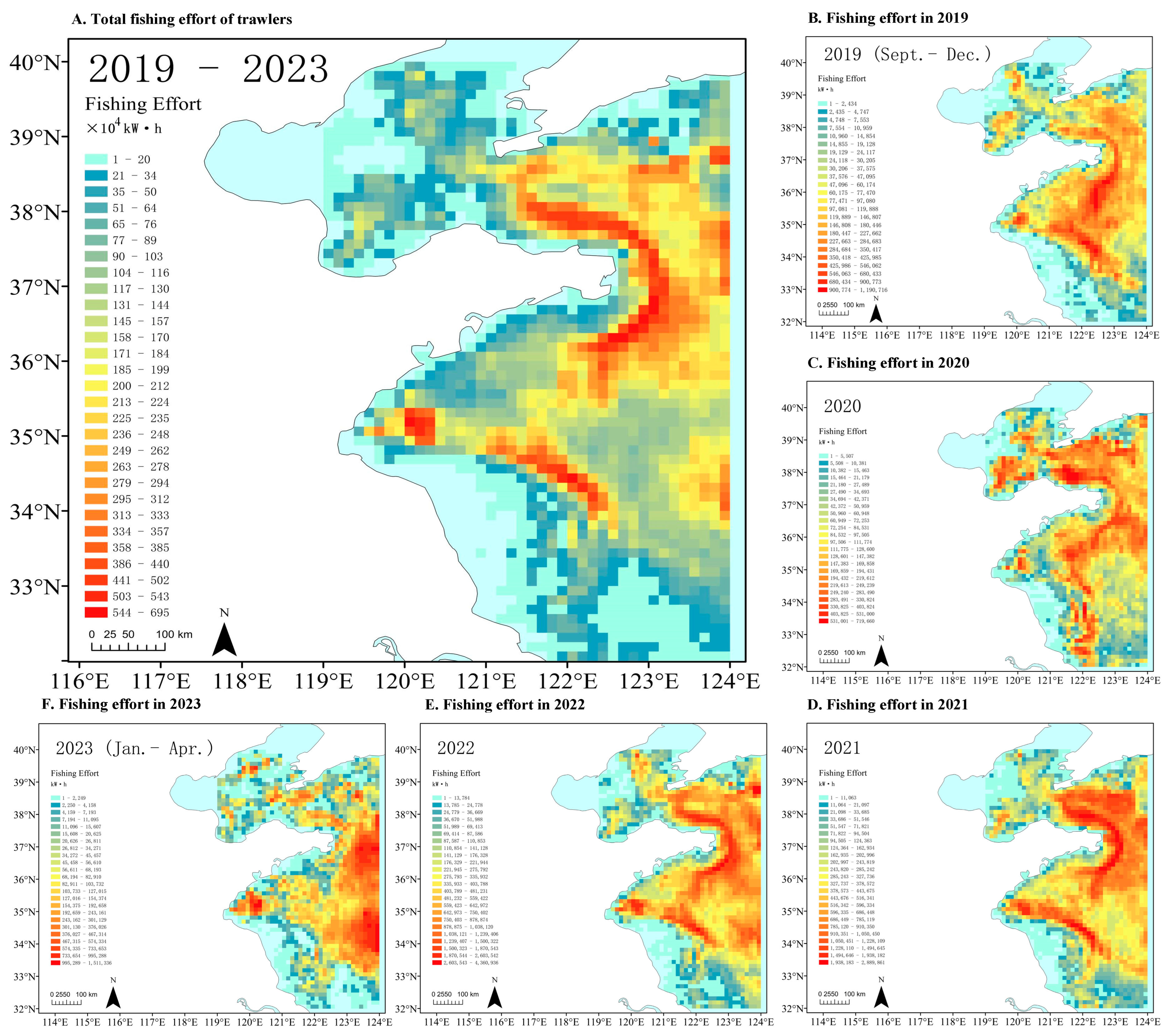
The spatial distribution of fishing effort was primarily concentrated in three key areas: 121° E~124° E, 35.5° N~39° N; 119.7° E~122.7° E, 33.8° N~35.5° N; and 123° E~124° E, 33.5° N~35° N.

(3)

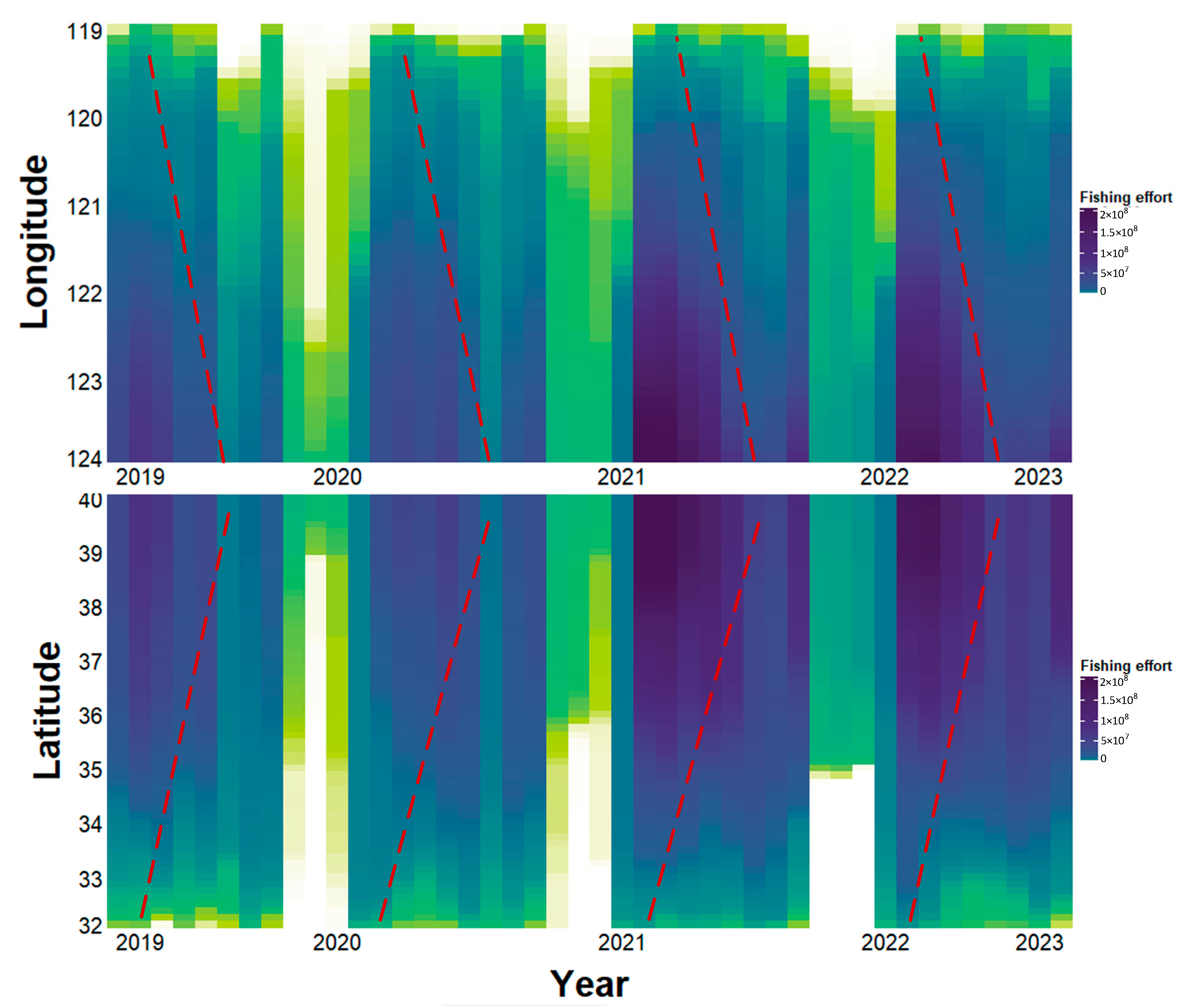
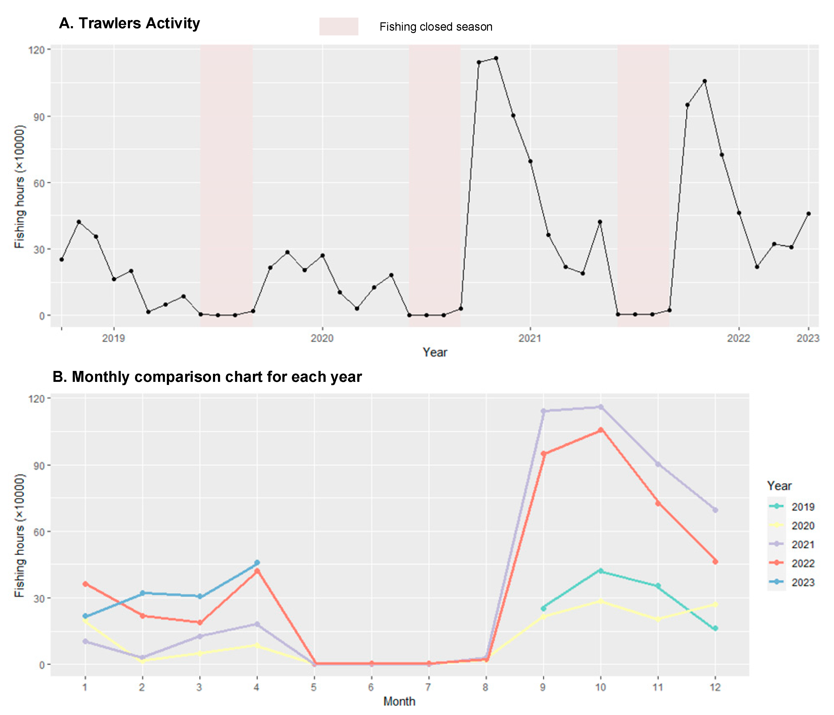
The temporal distribution exhibited periodic variations, which were closely associated with human activities such as the celebration of the Lunar New Year and the periods closed to fishing. The slope of the change in fishing effort concerning latitude distribution was approximately 2, whereas for longitude distribution, it was approximately −1.25.

The results of the proposed fishing behavior recognition model can intuitively reflect fishing activities and footprints. The estimated fishing effort, regarded as a precision input factor, could be combined with output factors, providing more accurate references for the assessment of fishing capacity. The integration with biological population information provides a valuable reference for a total allowable catch system. Meanwhile, this study assists in policy implementation, including supporting the law enforcement and supervision of fisheries, facilitating the control of marine fishing input intensity, and promoting the implementation of catch quota systems.

Further research is planned to take place, investigating the fishing behavior and fishing effort of purse seine and drift net fishing vessels. Additionally, researchers are currently collecting catch data from the Bohai Sea and the Yellow Sea to prepare for the assessment of fishing capacity.

References

1. FAO. The State of World Fisheries and Aquaculture, Contributing to Food Security and Nutrition for All; FAO: Rome, Italy, 2016. [Google Scholar]
2. Jason, S.L.; Reg, A.W. Global ecosystem overfishing: Clear delineation within real limits to production. Sci. Adv. 2019, 5, eaav0474. [Google Scholar]
3. FAO. The State of World Fisheries and Aquaculture; Food and Agriculture Organization of the United Nations: Rome, Italy, 2022. [Google Scholar]
4. Su, S.; Tang, Y.; Chang, B.; Zhu, W.; Chen, Y. Evolution of marine fisheries management in China from 1949 to 2019: How did China get here and where does China go next. Fish Fish. 2020, 21, 435–452. [Google Scholar] [CrossRef]
5. Zhang, X.; Vincent, A.C.J. China’s policies on bottom trawl fisheries over seven decades (1949–2018). Mar. Pol. 2020, 122, 104256. [Google Scholar] [CrossRef]
6. Bian, X.D.; Wan, R.J.; Jin, X.S.; Shan, X.J.; Guan, L.S. Ichthyoplankton Succession and Assemblage Structure in the Bohai Sea During the Past 30 Years Since the 1980s. Prog. Fish. Sci. 2018, 39, 1–15. [Google Scholar]
7. Shen, C.; Chen, T. Impact of fuel subsidies on bottom trawl fishery operation in China. Mar. Pol. 2022, 138, 104977. [Google Scholar] [CrossRef]
8. Andrew, N.L.; Béné, C.; Hall, S.J.; Allison, E.H.; Heck, S.; Ratner, B.D. Diagnosis and management of small-scale fisheries in developing countries. Fish Fish. 2007, 8, 227–240. [Google Scholar] [CrossRef]
9. Huang, S.; He, Y. Management of China’s capture fisheries: Review and prospect. Aquac. Fish. 2019, 4, 173–182. [Google Scholar] [CrossRef]
10. Mu, Y.; Yu, H.; Chen, J.; Zhu, Y. A qualitative appraisal of China’s efforts in fishing capacity management. J. Ocean Univ. China 2007, 6, 1–11. [Google Scholar] [CrossRef]
11. The National People’s Congress. Fisheries Law of the People’s Republic of China; The National People’s Congress: Beijing, China, 1986.
12. Zhao, L.; Sun, H.W.; Zheng, S.N.; Geng, R. Construction path of new fishery management system. Agric. Outlook 2016, 12, 41–46. [Google Scholar]
13. Ministry of Finance; Ministry of Agriculture. Regulations on the Management of Special Funds Using for Marine Fishermen to Change Their Jobs; Ministry of Finance: Beijing, China; Ministry of Agriculture: Beijing, China, 2003.
14. Ministry of Agriculture. Animal Husbandry and Fisheries, The State Council Opinions on Control Index of Offshore Fishing Vessels; The State Council: Beijing, China, 1987.
15. Ministry of Finance; Ministry of Agriculture State Price Bureau. Measures for Collection and Use of Fishery Resources Proliferation and Protection Fees; Ministry of Finance: Beijing, China; Ministry of Agriculture State Price Bureau: Beijing, China, 1988.
16. Ministry of Agriculture. Notice on Revising the Provisions on the Arrangement and Management of Fishing Season Production in the Main Fishing Grounds of East China Sea, Yellow Sea and Bohai Sea; Ministry of Agriculture: Beijing, China, 1995.
17. Su, M.; Wang, L.; Xiang, J.; Ma, Y. Adjustment trend of China’s marine fishery policy since 2011. Mar. Pol. 2021, 124, 104322. [Google Scholar] [CrossRef]
18. Zhang, Z.; Wu, S.; Li, S.; Cao, J.; Ge, S. Evaluation of the effectiveness of the implementation of the “dual control system” for fishing vessels in China and policy recommendations. China Fish. 2018, 4, 34–40. [Google Scholar]
19. Zhang, W.; Chang, Y.-C.; Zhang, L. Azn ocean community with a shared future: Conference report. Mar. Pol. 2020, 116, 103888. [Google Scholar] [CrossRef]
20. Butt, M.J.; Chang, Y.C.; Zulfiqar, K. A comparative analysis of the environmental policies in China and Pakistan: Developing a legal regime for sustainable ChinaPakistan economic corridor (CPEC) under the Belt and road initiative (BRI). IPRI J. 2021, 21, 83–122. [Google Scholar] [CrossRef]
21. Zhang, H. Fisheries cooperation in the SouthSouth China sea: Evaluating the options. Mar. Pol. 2018, 89, 67–76. [Google Scholar] [CrossRef]
22. Shen, H.; Huang, S. China’s policies and practice on combatting IUU in distant water fisheries. Aquac. Fish. 2021, 6, 27–34. [Google Scholar] [CrossRef]
23. Yin, J.; Xue, Y.; Li, Y.Z.; Zhang, C.L.; Xu, B.D.; Liu, Y.W.; Ren, Y.P.; Chen, Y. Evaluating the efficacy of fisheries management strategies in China for achieving multiple objectives under climate change. Ocean Coast. Manag. 2023, 245, 106870. [Google Scholar] [CrossRef]
24. Yang, H.J.; Peng, D.M.; Liu, H.H.; Mu, Y.T.; Kim, D.H. Is China’s Fishing Capacity Management Sufficient? Quantitative Assessment of China’s Efforts toward Fishing Capacity Management and Proposals for Improvement. J. Mar. Sci. Eng. 2022, 10, 1998. [Google Scholar]
25. Ministry of Agriculture. Notice on Further Strengthening the Control of Domestic Fishing Vessels and Implementing the Total Management of Marine Fishery Resources; Ministry of Agriculture: Beijing, China, 2017.
26. Su, X.; Chen, X. Comparative study for input control output control in fishery management. Trans. Oceanol. Limnol. 2021, 3, 136–144. [Google Scholar]
27. Ministry of Agriculture. Notice on Adjusting Domestic Fishery Fishing and Aquaculture Oil Price Subsidy Policies to Promote the Sustainable and Healthy Development of Fisheries; Ministry of Agriculture: Beijing, China, 2015.
28. Ou, C.H.; Tseng, H.S. The fishery agreements and management systems in the East China Sea. Ocean Coast. Manag. 2010, 5, 279–288. [Google Scholar] [CrossRef]
29. Rosenberg, D. Managing the resources of the China Seas: China’s bilateral fisheries agreements with Japan, South Korea, and Vietnam. Asia-Pac. J. 2005, 3, 24–29. [Google Scholar]
30. Ding, Q.; Shan, X.J.; Jin, X.S.; Gorfin, E.H.; Guan, L.S.; Yang, T. Evolution of China’s Total Allowable Catch (TAC) system: Review and way forward. Mar. Policy 2023, 147, 105390. [Google Scholar] [CrossRef]
31. Li, Y.Z.; Sun, M.; Ren, Y.P.; Chen, Y. Fisher behavior matters: Harnessing spatio-temporal fishing effort information to support China’s fisheries management. Ocean Coast. Manag. 2021, 210, 105665. [Google Scholar] [CrossRef]
32. Mohamed, S.K.; Aitor, F.; Jose, L.S.L. Daily variation of fishing effort and ex-vessel prices in a western Mediterranean multi-species fishery: Implications for sustainable management. Mar. Policy 2015, 61, 187–195. [Google Scholar]
33. Vanessa, S.; Francese, M.; Guillaume, B.; Gwenael, C.; Matthew, C.; Romain, C.H.; Geraldine, C.; Mark, D.; Oscar, E.; Ruth, H.; et al. Spatial assessment of fishing effort around European marine reserves: Implications for successful fisheries management. Mar. Pollut. Bull. 2008, 56, 2018–2026. [Google Scholar]
34. Hugo, P.; Christopher, K.P.; Miguel, M.; Marco, S.; Karen, A.B.; Frederic, V. The Portuguese industrial pelagic longline fishery in the Northeast Atlantic: Catch composition, spatio-temporal dynamics of fishing effort, and target species catch rates. Fish. Res. 2023, 264, 106730. [Google Scholar]
35. Ashley, T.; Colin, J.D.; Carolyn, M.I.; Stuart, E.J.; Greg, G.S.; Christopher, T.S.; Brett, T.P.; Olaf, P.J. Estimating fishing effort across the landscape: A spatially extensive approach using models to integrate multiple data sources. Fish. Res. 2021, 233, 105768. [Google Scholar]
36. Francois, B.; Rasmus, N.; Clara, U.; Josefine, E.; Henrik, D. Detailed mapping of fishing effort and landings by coupling fishing logbooks with satellite-recorded vessel geo-location. Fish. Res. 2010, 106, 41–53. [Google Scholar]
37. Moore, J.E. An interview-based approach to assess marine mammal and sea turtle captures in artisanal fisheries. Biol. Conserv. 2010, 143, 795–805. [Google Scholar] [CrossRef]
38. Alfaro-Cordova, E.; Del Solar, A.; Alfaro-Shigueto, J.; Mangel, J.C.; Diaz, B.; Carrillo, O.; Sarmiento, D. Captures of manta and devil rays by small-scale gillnet fisheries in northern Peru. Fish. Res. 2017, 195, 28–36. [Google Scholar] [CrossRef]
39. Candan, U.S.; Tomoharu, E.; Suzanne, K.; Heidi, D. Prediction of fishing effort distributions using boosted regression trees. Ecol. Appl. 2014, 24, 71–83. [Google Scholar]
40. Benjamin, D.W.; Patrick, D.O.; Natalie, C.B. Improving effort estimates and informing temporal distribution of recreational salmon fishing in British Columbia, Canada using high-frequency optical imagery data. Fish. Res. 2022, 249, 106251. [Google Scholar]
41. Malvestuto, S.P. Sampling the recreational fishery. In Fisheries Techniques, 2nd ed.; American Fisheries Society: Bathesda, MD, USA, 1996; pp. 591–623. [Google Scholar]
42. Parkinson, E.A.; Berkowitz, J.; Bull, C.J. Sample size requirements for detecting changes in some fisheries statistics from small trout lakes. N. Am. J. Fish. Manag. 1988, 8, 181–190. [Google Scholar] [CrossRef]
43. Jaeyoon, P.; Jungsam, L.; Katherine, S.; Timothy, H.; Brian, A.W.; Nathan, A.M.; Kenji, T.; Hiroshi, K.; Yoshioki, O.; David, A.K. Illuminating dark fishing fleets in North Korea. Sci. Adv. 2020, 6, 30. [Google Scholar]
44. Ganggang, G.; Wei, F.; Jialun, X.; Shengmao, Z.; Heng, Z.; Fenghua, T.; Tianfei, C. Identification for operating pelagic light-fishing vessels based on NPP/VIIRS low light imaging data. Trans. CSAE 2017, 33, 245–251. [Google Scholar]
45. Brett, T.P.; Scott, B. Estimating fishing effort from remote traffic counters: Opportunities and challenges. Fish. Res. 2018, 204, 231–238. [Google Scholar]
46. Mullowney, D.R.; Dawe, E.G. Development of performance indices for the Newfoundland and Labrador snow crab (Chionoecetes opilio) fishery using data from a vessel monitoring system. Fish. Res. 2009, 100, 248–254. [Google Scholar] [CrossRef]
47. Russo, T.; D’Andrea, L.; Parisi, A.; Martinelli, M.; Belardinelli, A.; Boccoli, F.; Cignini, I.; Tordoni, M.; Cataudella, S. Assessing the fishing footprint using data integrated from different tracking devices: Issues and opportunities. Ecol. Indic. 2016, 69, 818–827. [Google Scholar] [CrossRef]
48. Pascal, T.; Joseph, M.; Christian, M.; Kerstin, S.S. AIS and VMS ensemble can address data gaps on fisheries for marine spatial planning. Sustainability 2021, 13, 3769. [Google Scholar]
49. Gerritsen, H.D.; Minto, C.; Lordan, C. How much of the seabed is impacted by mobile fishing gear? Absolute estimates from Vessel Monitoring System (VMS) point data. ICES J. Mar. Sci. 2013, 70, 523–531. [Google Scholar]
50. Yan, Z.; He, R.; Ruan, X.; Yang, H. Footprints of fishing vessels in Chinese waters based on automatic identification system data. J. Sea Res. 2022, 187, 102255. [Google Scholar] [CrossRef]
51. Zhang, H.; Yang, S.-L.; Fan, W.; Shi, H.-M.; Yuan, S.-L. Spatial analysis of the fishing behaviour of tuna purse seiners in the western and central Pacific based on vessel trajectory data. J. Mar. Sci. Eng. 2021, 9, 322. [Google Scholar] [CrossRef]
52. Craig, M.M.; Sunny, E.T.; Simon, J.; Paul, D.E.; Carla, A.H. Estimating high resolution trawl fishing effort from satellite-based vessel monitoring system data. ICES J. Mar. Sci. 2006, 64, 248–255. [Google Scholar]
53. Peel, D.; Good, N.M. A hidden markov model approach for determining vessel activity from vessel monitoring system data. Can. J. Fish. Aquat. Sci. 2011, 68, 1252–1264. [Google Scholar] [CrossRef]
54. Bertrand, S.; Burgos, J.M.; Gerlotto, F. Lévy trajectories of Peruvian purse-seiners as an indicator of the spatial distribution of anchovy (Engraulis ringens). ICES J. Mar. Sci. 2005, 62, 477–482. [Google Scholar] [CrossRef]
55. Lee, J.; South, A.B.; Jennings, S. Developing reliable, repeatable and accessible methods to provide high-resolution estimates of fishing effort distributions from vessel monitoring system (VMS) data. ICES J. Mar. Sci. 2010, 67, 1260–1271. [Google Scholar] [CrossRef]
56. Faustinato, B.; Marie, P.E.; Jérôme, G.S. Estimating fishing effort in small-scale fisheries using GPS tracking data and random forests. Ecol. Indic. 2021, 123, 107321. [Google Scholar]
57. Yang, S.L.; Zhang, S.M.; Zhou, W.F.; Cui, X.S.; Zhang, B.B.; Fan, W. Calculating the fishing effort of longline fishing vessel in the western and central pacific ocean using AIS. Trans. Chin. Soc. Agric. Eng. 2020, 36, 198–203. [Google Scholar]
58. Ning, Y. Research on the Behavior Identification Method of Fishing Vessels Based on Deep Learning. Ph.D. Thesis, Lanzhou University, Lanzhou, China, 2020. [Google Scholar]
59. David, A.K.; Juan, K.; Timothy, H. Tracking the global footprint of fisheries. Science 2018, 359, 904–908. [Google Scholar]
60. Peng, J.; Mao, M.; Xia, M. Dynamics of wave generation and dissipation processes during cold were events in the Bohai Sea. Estuar. Coast. Shelf Sci. 2023, 280, 108161. [Google Scholar] [CrossRef]
61. Choi, J. Assessing the need for the designation of the Yellow Sea Particularly Sensitive Sea Area (PSSA). Mar. Policy 2022, 137, 104971. [Google Scholar] [CrossRef]
62. Chen, R.; Wu, X.; Liu, B.; Wang, Y.; Gao, Z. Mapping coastal fishing grounds and assessing the effectiveness of fishery regulation measures with AIS data: A case study of the sea area around the Bohai Strait, China. Ocean Coast. Manag. 2022, 223, 106136. [Google Scholar] [CrossRef]
63. Ke, G.L.; Meng, Q.; Finley, T.; Wang, T.F.; Chen, W.; Ma, W.D.; Ye, Q.W.; Liu, T.Y. LightGBM: A highly efficient gradient boosting decision tree. In Proceedings of the 31st Conference on Neural Information Processing Systems (NIPS 2017), Long Beach, CA, USA, 4–9 December 2017. [Google Scholar]
64. Zhang, Y.; Gao, S.C.; Cai, P.X.; Lei, Z.Y.; Wang, Y.R. Information entropy-based differential evolution with extremely randomized trees and LightGBM for protein structural class prediction. Appl. Soft Comput. 2023, 136, 110064. [Google Scholar] [CrossRef]
65. Li, S.; Chen, H.; Wang, M.; Heidari, A.A.; Mirjalili, S. Slime mould algorithm: A new method for stochastic optimization. Future Gener. Comput. Syst. 2020, 111, 300–323. [Google Scholar] [CrossRef]
66. Chawla, N.V.; Bowyer, K.W.; Hall, L.O.; Kegelmeyer, W.P. SMOTE: Synthetic minority over-sampling technique. J. Artif. Intell. Res. 2002, 16, 321–357. [Google Scholar] [CrossRef]
67. Li, D.; Chen, Y.F.; Zhang, K.F.; Li, Z.B. Mounting Behaviour Recognition for Pigs Based on Deep Learning. Sensors 2019, 19, 4924. [Google Scholar] [CrossRef]
68. Zhang, S.M.; Cui, X.S.; Wu, Y.M.; Zheng, Q.; Wang, X.; Fan, W. Analyzing space-time characteristics of Xiangshan trawling based on Beidou Vessel Monitoring System Data. Trans. Chin. Soc. Agric. Eng. 2015, 31, 151–156. [Google Scholar]
69. FAO. Definition of Some Key Terms [EB/OL]. Fisheries and Aquaculture Department. 1997. Available online: https://www.fao.org/docrep/003/w4230e/w4230e09.htm (accessed on 20 December 2023).
70. Tiralongo, F.; Messina, G.; Lombardo, B.M. Discards of elasmobranchs in a trammel net fishery targeting cuttlefish, Sepia officinalis Linnaeus, 1758, along the coast of Sicily (central Mediterranean Sea). Reg. Stud. Mar. Sci. 2018, 20, 60–63. [Google Scholar] [CrossRef]
71. Tiralongo, F.; Mancini, E.; Ventura, D.; De Malerbe, S.; Paladini De Mendoza, F.; Sardone, M.; Arciprete, R.; Massi, D.; Marcelli, M.; Fiorentino, F.; et al. Commercial catches and discards composition in the central Tyrrhenian Sea: A multispecies quantitative and qualitative analysis from shallow and deep bottom trawling. Mediterr. Mar. Sci. 2021, 22, 521–531. [Google Scholar] [CrossRef]
Figure 1. Location of the study sea area.
Jmse 12 00064 g001
Figure 2. Location of the annotated ports.
Jmse 12 00064 g002
Figure 3. Flow chart depicting the fishing behavior recognition model with SMA-LightGBM.
Jmse 12 00064 g003
Figure 4. Diagram of the fluxes in the training and testing processes involved in SMA-LightGBM.
Jmse 12 00064 g004
Figure 5. The spatial distribution of trawler fishing effort. (A) Total fishing effort from September 2019 to April 2023. (B) Fishing effort in 2019 (from September to December). (C) Fishing effort in 2020. (D) Fishing effort in 2021. (E) Fishing effort in 2022. (F) Fishing effort in 2023 (from January to April).
Jmse 12 00064 g005
Figure 6. The temporal distribution of trawler fishing effort. The red dashed lines signified the temporal variations of fishing effort in longitude and latitude dimensions.
Jmse 12 00064 g006
Figure 7. Time series chart of fishing hours by month. (A) Time series of trawlers fishing hours by month. (B) Monthly comparison chart for 5 years.
Jmse 12 00064 g007