
Model for Underwater Acoustic Target Recognition with Attention Mechanism Based on Residual Concatenate
Abstract
:1. Introduction
2. System Overview
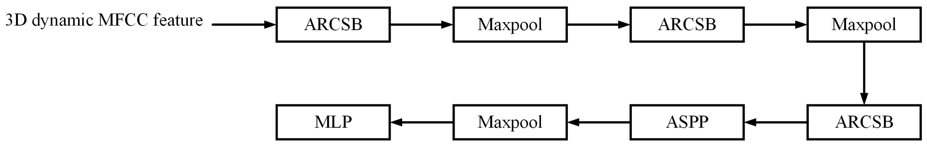
2.1. Construction of the Proposed Model
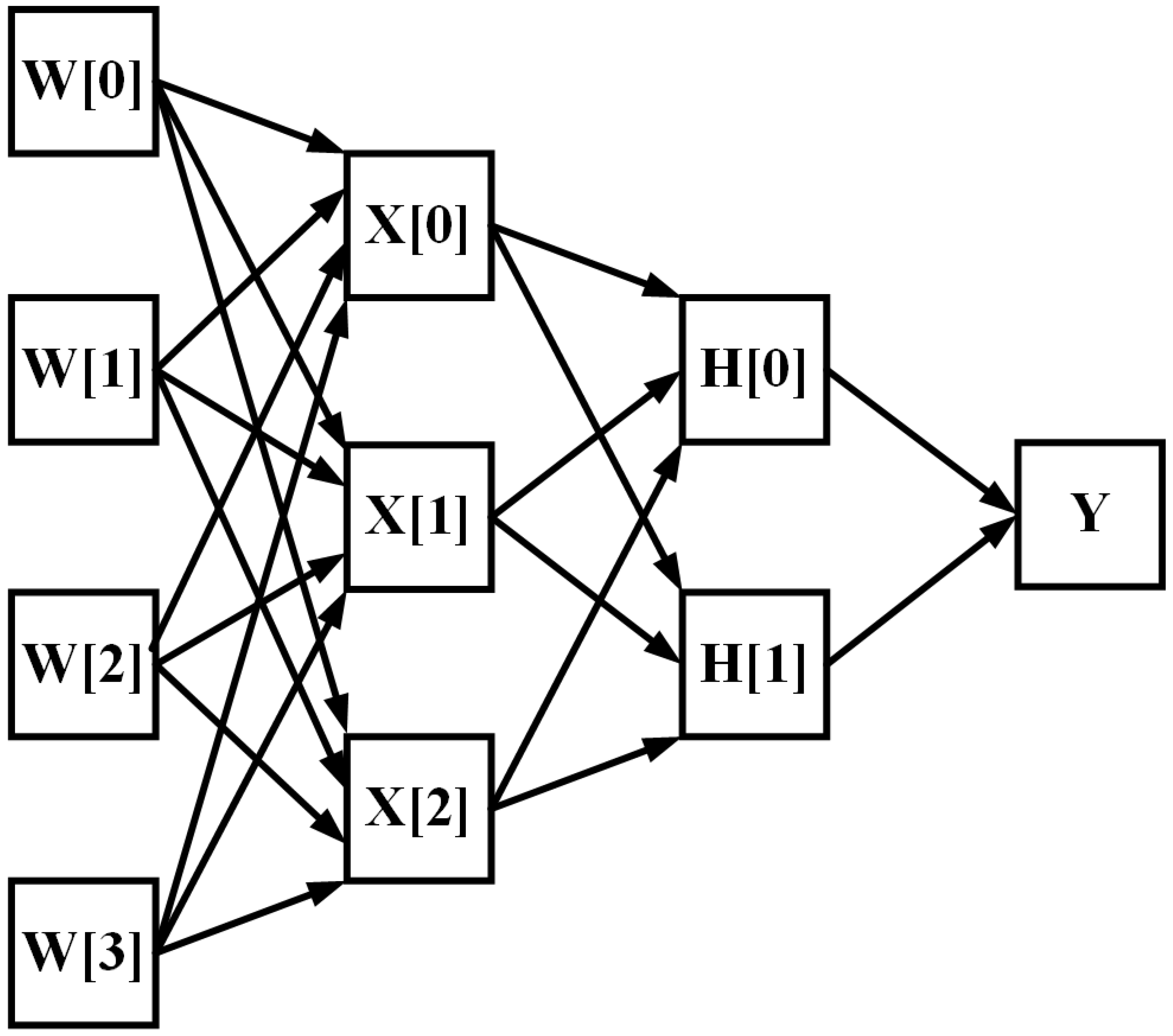
ARescat Network Model (Refer to Figure 1)
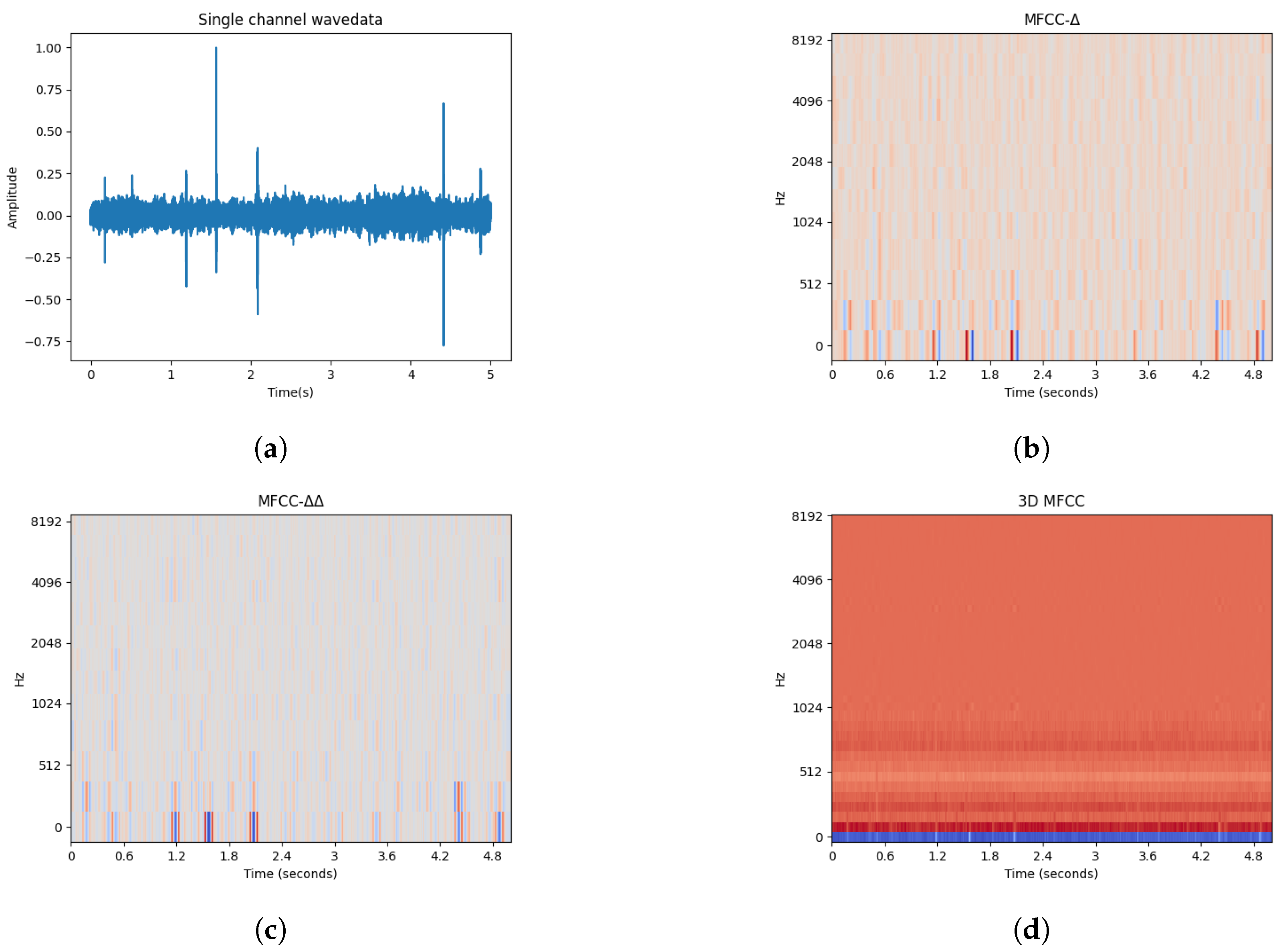
2.2. 3D MFCC Feature Extraction Methods
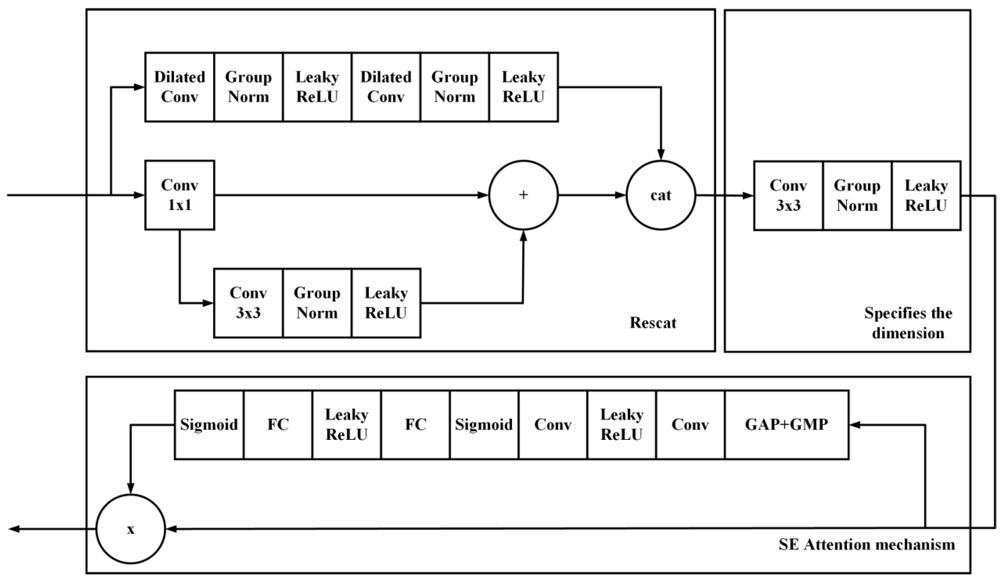
2.3. ARCSB Network
2.3.1. Structure and Components
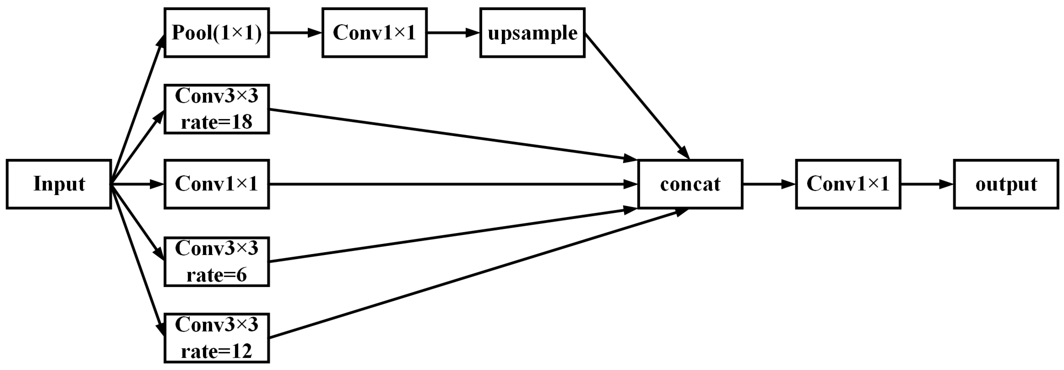
2.3.2. ASPP (Atrous Spatial Pyramid Pooling)
2.4. MLP (Multilayer Perceptron)
2.5. Focal Loss
3. Experimentation and Analysis
3.1. Dataset Description
3.2. Hyperparameter Configuration and Loss Function Design
3.3. Performance Evaluation
3.3.1. Model Performance Insights
3.3.2. Ablation Experiments on Network Modules
3.3.3. Role of Loss Function in Model Performance
3.3.4. Characterization Ablation Experiments
3.3.5. Comparison between Different Models
3.3.6. Accuracy Comparison of Various Models
4. Conclusions
Author Contributions
Funding
Institutional Review Board Statement
Data Availability Statement
Conflicts of Interest
Abbreviations
| ARescat | Attention Mechanism Residual Concatenate Network |
| SE | Squeeze-Excitation |
| ResNet | Residual Network |
| MFCC | Mel-frequency Cepstrum Coefficient |
| CQT | Constant-Q Transform |
| DEMON | Detection of Envelope Modulation On Noise |
| LOFAR | Low-frequency Analyzer and Recorder |
| 3D MFCC | 3D dynamic Mel-frequency Cepstrum Coefficient |
| MSRDN | Multiscale Residual Deep Neural Network |
| ARCSB | Attention Mechanism Residual Concatenate Specify Dimensions Block |
| ASPP | Atrous Spatial Pyramid Pooling |
| MLP | Multilayer Perceptron |
| FC | Fully Connected |
| Rescat | Residual Concatenate |
| CRNN | Convolutional Recurrent Neural Network |
References
- Kamal, S.; Mohammed, S.K.; Pillai, P.S.; Supriya, M. Deep learning architectures for underwater target recognition. In Proceedings of the 2013 Ocean Electronics (SYMPOL), IEEE, Kochi, India, 23–25 October 2013; pp. 48–54. [Google Scholar] [CrossRef]
- Cao, X.; Zhang, X.; Yu, Y.; Niu, L. Deep learning-based recognition of underwater target. In Proceedings of the 2016 IEEE International Conference on Digital Signal Processing (DSP), IEEE, Beijing, China, 16–18 October 2016; pp. 89–93. [Google Scholar] [CrossRef]
- Li, C.; Liu, Z.; Ren, J.; Wang, W.; Xu, J. A feature optimization approach based on inter-class and intra-class distance for ship type classification. Sensors 2020, 20, 5429. [Google Scholar] [CrossRef] [PubMed]
- Yang, H.; Shen, S.; Yao, X.; Sheng, M.; Wang, C. Competitive deep-belief networks for underwater acoustic target recognition. Sensors 2018, 18, 952. [Google Scholar] [CrossRef] [PubMed]
- Irfan, M.; Jiangbin, Z.; Ali, S.; Iqbal, M.; Masood, Z.; Hamid, U. DeepShip: An underwater acoustic benchmark dataset and a separable convolution based autoencoder for classification. Expert Syst. Appl. 2021, 183, 115270. [Google Scholar] [CrossRef]
- Permana, S.D.H.; Bintoro, K.B.Y. Implementation of Constant-Q Transform (CQT) and Mel Spectrogram to converting Bird’s Sound. In Proceedings of the 2021 IEEE International Conference on Communication, Networks and Satellite (COMNETSAT). IEEE, Purwokerto, Indonesia, 17–18 July 2021; pp. 52–56. [Google Scholar] [CrossRef]
- Wei, X.; Gang-Hu, L.; Wang, Z. Underwater target recognition based on wavelet packet and principal component analysis. Comput. Simul. 2011, 28, 8–290. [Google Scholar]
- Azimi-Sadjadi, M.R.; Yao, D.; Huang, Q.; Dobeck, G.J. Underwater target classification using wavelet packets and neural networks. IEEE Trans. Neural Netw. 2000, 11, 784–794. [Google Scholar] [CrossRef] [PubMed]
- Chen, Y.; Xu, X. The research of underwater target recognition method based on deep learning. In Proceedings of the 2017 IEEE International Conference on Signal Processing, Communications and Computing (ICSPCC). IEEE, Xiamen, China, 22–25 October 2017; pp. 1–5. [Google Scholar] [CrossRef]
- Liu, F.; Shen, T.; Luo, Z.; Zhao, D.; Guo, S. Underwater target recognition using convolutional recurrent neural networks with 3-D Mel-spectrogram and data augmentation. Appl. Acoust. 2021, 178, 107989. [Google Scholar] [CrossRef]
- Luo, X.; Zhang, M.; Liu, T.; Huang, M.; Xu, X. An underwater acoustic target recognition method based on spectrograms with different resolutions. J. Mar. Sci. Eng. 2021, 9, 1246. [Google Scholar] [CrossRef]
- Li, Y.; Gao, P.; Tang, B.; Yi, Y.; Zhang, J. Double feature extraction method of ship-radiated noise signal based on slope entropy and permutation entropy. Entropy 2021, 24, 22. [Google Scholar] [CrossRef]
- Zhang, L.; Wu, D.; Han, X.; Zhu, Z. Feature extraction of underwater target signal using mel frequency cepstrum coefficients based on acoustic vector sensor. J. Sens. 2016, 2016, 7864213. [Google Scholar] [CrossRef]
- Yang, S.; Xue, L.; Hong, X.; Zeng, X. A Lightweight Network Model Based on an Attention Mechanism for Ship-Radiated Noise Classification. J. Mar. Sci. Eng. 2023, 11, 432. [Google Scholar] [CrossRef]
- Gou, J.; Yu, B.; Maybank, S.J.; Tao, D. Knowledge distillation: A survey. Int. J. Comput. Vis. 2021, 129, 1789–1819. [Google Scholar] [CrossRef]
- Le Gall, Y.; Bonnel, J. Separation of moving ship striation patterns using physics-based filtering. In Proceedings of the Meetings on Acoustics, Montreal, QC, Canada, 2–7 June 2013; AIP Publishing: Melville, NY, USA, 2013; Volume 19. [Google Scholar] [CrossRef]
- Kuz’kin, V.; Kuznetsov, G.; Pereselkov, S.; Grigor’ev, V. Resolving power of the interferometric method of source localization. Phys. Wave Phenom. 2018, 26, 150–159. [Google Scholar] [CrossRef]
- Ehrhardt, M.; Pereselkov, S.; Kuz’kin, V.; Kaznacheev, I.; Rybyanets, P. Experimental observation and theoretical analysis of the low-frequency source interferogram and hologram in shallow water. J. Sound Vib. 2023, 544, 117388. [Google Scholar] [CrossRef]
- Pereselkov, S.A.; Kuz’kin, V.M. Interferometric processing of hydroacoustic signals for the purpose of source localization. J. Acoust. Soc. Am. 2022, 151, 666–676. [Google Scholar] [CrossRef] [PubMed]
- He, K.; Zhang, X.; Ren, S.; Sun, J. Deep residual learning for image recognition. In Proceedings of the IEEE Conference on Computer Vision and Pattern Recognition, Las Vegas, NV, USA, 26 June–1 July 2016; pp. 770–778. [Google Scholar] [CrossRef]
- Huang, G.; Sun, Y.; Liu, Z.; Sedra, D.; Weinberger, K.Q. Deep networks with stochastic depth. In Proceedings of the Computer Vision–ECCV 2016: 14th European Conference, Amsterdam, The Netherlands, 11–14 October 2016, Proceedings, Part IV 14; Springer: Berlin/Heidelberg, Germany, 2016; pp. 646–661. [Google Scholar] [CrossRef]
- Tian, S.; Chen, D.; Wang, H.; Liu, J. Deep convolution stack for waveform in underwater acoustic target recognition. Sci. Rep. 2021, 11, 9614. [Google Scholar] [CrossRef] [PubMed]
- Xue, L.; Zeng, X.; Jin, A. A novel deep-learning method with channel attention mechanism for underwater target recognition. Sensors 2022, 22, 5492. [Google Scholar] [CrossRef] [PubMed]
- Zhufeng, L.; Xiaofang, L.; Na, W.; Qingyang, Z. Present status and challenges of underwater acoustic target recognition technology: A review. Front. Phys. 2022, 10, 1044890. [Google Scholar] [CrossRef]
- Chen, S.; Tan, X.; Wang, B.; Lu, H.; Hu, X.; Fu, Y. Reverse attention-based residual network for salient object detection. IEEE Trans. Image Process. 2020, 29, 3763–3776. [Google Scholar] [CrossRef]
- Lu, Z.; Xu, B.; Sun, L.; Zhan, T.; Tang, S. 3-D channel and spatial attention based multiscale spatial–spectral residual network for hyperspectral image classification. IEEE J. Sel. Top. Appl. Earth Obs. Remote Sens. 2020, 13, 4311–4324. [Google Scholar] [CrossRef]
- Hong, F.; Liu, C.; Guo, L.; Chen, F.; Feng, H. Underwater acoustic target recognition with a residual network and the optimized feature extraction method. Appl. Sci. 2021, 11, 1442. [Google Scholar] [CrossRef]
- Jiang, K.; Wang, Z.; Yi, P.; Chen, C.; Huang, B.; Luo, Y.; Ma, J.; Jiang, J. Multi-scale progressive fusion network for single image deraining. In Proceedings of the IEEE/CVF Conference on Computer Vision and Pattern Recognition, Seattle, WA, USA, 13–19 June 2020; pp. 8346–8355. [Google Scholar] [CrossRef]
- Woo, S.; Park, J.; Lee, J.Y.; Kweon, I.S. Cbam: Convolutional block attention module. In Proceedings of the European Conference on Computer Vision (ECCV), Munich, Germany, 8–14 September 2018; pp. 3–19. [Google Scholar] [CrossRef]
- Hu, J.; Shen, L.; Sun, G. Squeeze-and-excitation networks. In Proceedings of the IEEE Conference on Computer Vision and Pattern Recognition, Salt Lake City, UT, USA, 18–23 June 2018; pp. 7132–7141. [Google Scholar] [CrossRef]
- Lin, T.Y.; Goyal, P.; Girshick, R.; He, K.; Dollár, P. Focal loss for dense object detection. In Proceedings of the IEEE International Conference on Computer Vision, Venice, Italy, 22–29 October 2017; pp. 2980–2988. [Google Scholar] [CrossRef]
- Chen, X.; Liang, C.; Huang, D.; Real, E.; Wang, K.; Liu, Y.; Pham, H.; Dong, X.; Luong, T.; Hsieh, C.J.; et al. Symbolic discovery of optimization algorithms. arXiv 2023, arXiv:2302.06675. [Google Scholar] [CrossRef]
- Santos-Domínguez, D.; Torres-Guijarro, S.; Cardenal-López, A.; Pena-Gimenez, A. ShipsEar: An underwater vessel noise database. Appl. Acoust. 2016, 113, 64–69. [Google Scholar] [CrossRef]
- Khishe, M. Drw-ae: A deep recurrent-wavelet autoencoder for underwater target recognition. IEEE J. Ocean. Eng. 2022, 47, 1083–1098. [Google Scholar] [CrossRef]
- Kamalipour, M.; Agahi, H.; Khishe, M.; Mahmoodzadeh, A. Passive ship detection and classification using hybrid cepstrums and deep compound autoencoders. Neural Comput. Appl. 2023, 35, 7833–7851. [Google Scholar] [CrossRef]
- Jia, H.; Khishe, M.; Mohammadi, M.; Rashidi, S. Deep cepstrum-wavelet autoencoder: A novel intelligent sonar classifier. Expert Syst. Appl. 2022, 202, 117295. [Google Scholar] [CrossRef]
- Wu, J.; Li, P.; Wang, Y.; Lan, Q.; Xiao, W.; Wang, Z. VFR: The Underwater Acoustic Target Recognition Using Cross-Domain Pre-Training with FBank Fusion Features. J. Mar. Sci. Eng. 2023, 11, 263. [Google Scholar] [CrossRef]


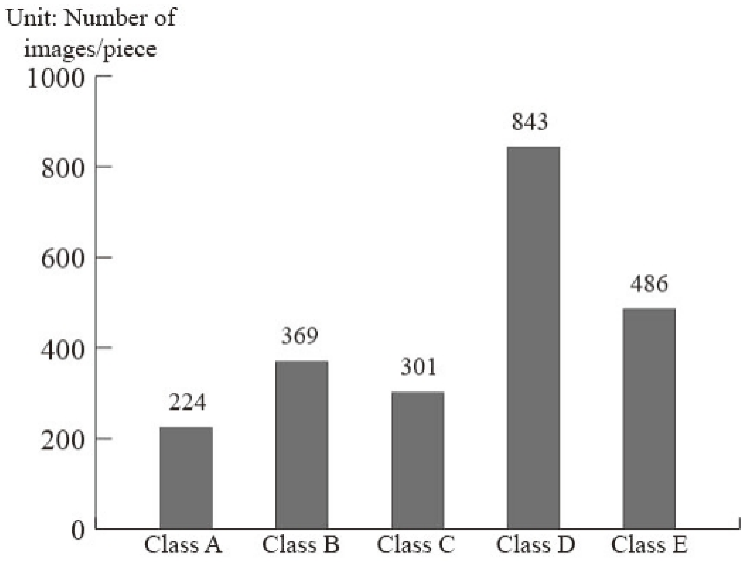
| Class | Target | The Number of Samples |
|---|---|---|
| Class A | Background noise recordings | 224 |
| Class B | Dredgers/Fishing boats/Mussel boats/Trawlers/Tugboats | 52/101/144/32/40 |
| Class C | Motorboats/Pilot boats/Sailboats | 196/26/79 |
| Class D | Passenger ferries | 843 |
| Class E | Ocean liners/Ro-ro vessels | 186/300 |
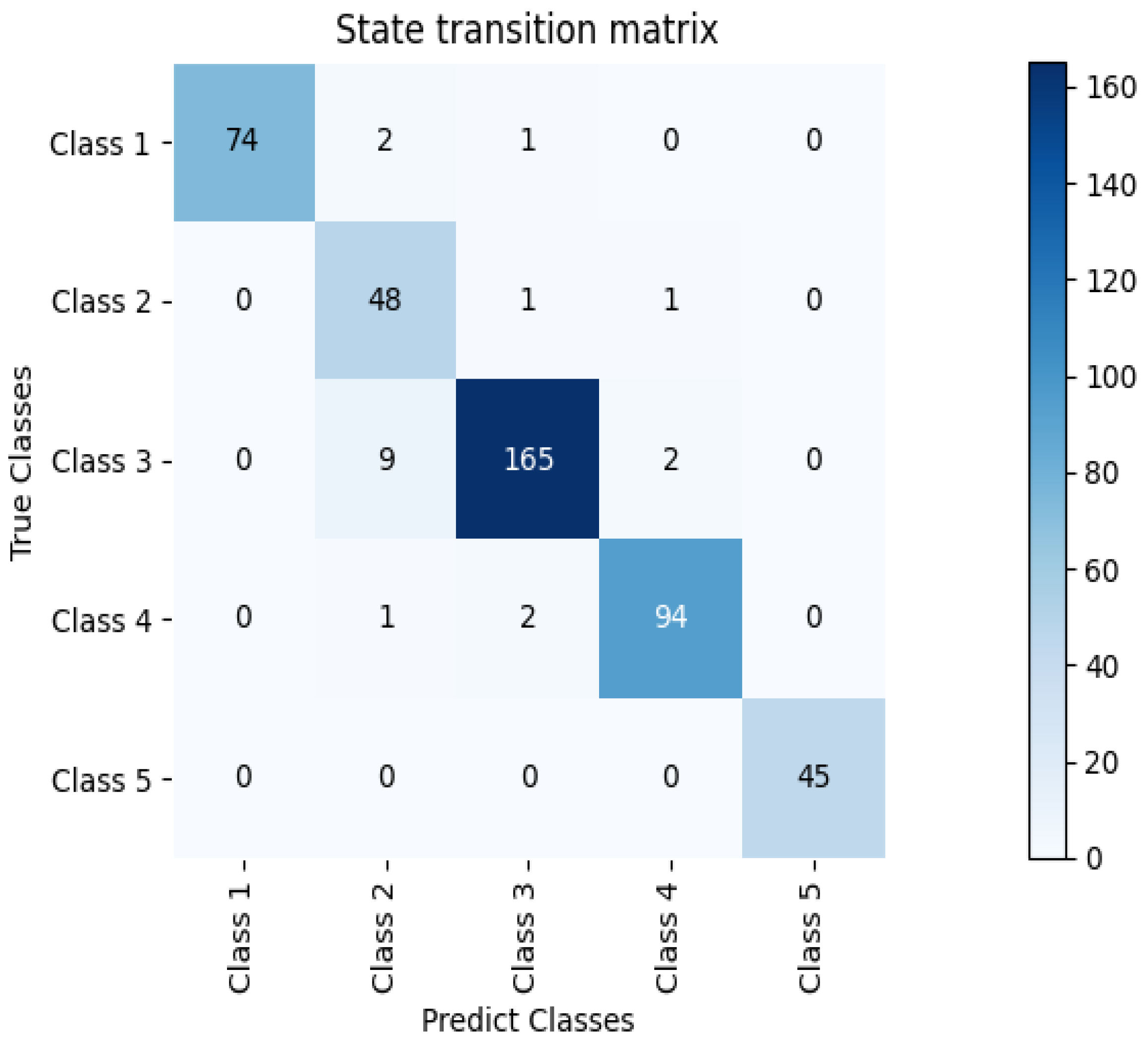
| Class | Precision | Recall | F1-Score | Support |
|---|---|---|---|---|
| Class A | 0.960 | 1.000 | 0.984 | 74 |
| Class B | 0.958 | 0.804 | 0.867 | 60 |
| Class C | 0.937 | 0.984 | 0.959 | 169 |
| Class D | 0.970 | 0.966 | 0.970 | 97 |
| Class E | 1.000 | 1.000 | 1.000 | 45 |
| Average | 0.958 | 0.958 | 0.958 | 445 |
| Model | Class | Precision | Recall | F1-Score | Support |
|---|---|---|---|---|---|
| ARescat | Class A | 0.960 | 1.000 | 0.984 | 74 |
| Class B | 0.958 | 0.804 | 0.867 | 60 | |
| Class C | 0.937 | 0.984 | 0.959 | 169 | |
| Class D | 0.970 | 0.966 | 0.970 | 97 | |
| Class E | 1.000 | 1.000 | 1.000 | 45 | |
| Average | 0.958 | 0.958 | 0.958 | 445 | |
| ARescat-1 | Class A | 0.932 | 1.000 | 0.960 | 74 |
| Class B | 0.921 | 0.754 | 0.825 | 60 | |
| Class C | 0.916 | 0.965 | 0.941 | 169 | |
| Class D | 0.979 | 0.930 | 0.954 | 97 | |
| Class E | 1.000 | 1.000 | 1.000 | 45 | |
| Average | 0.939 | 0.939 | 0.939 | 445 | |
| ARescat-2 | Class A | 0.753 | 0.908 | 0.819 | 74 |
| Class B | 0.971 | 0.500 | 0.655 | 60 | |
| Class C | 0.806 | 0.952 | 0.883 | 169 | |
| Class D | 0.948 | 0.823 | 0.880 | 97 | |
| Class E | 1.000 | 0.956 | 0.981 | 45 | |
| Average | 0.857 | 0.857 | 0.857 | 445 |
| Model | Class | Precision | Recall | F1-Score | Support |
|---|---|---|---|---|---|
| ARescat | Class A | 0.960 | 1.000 | 0.984 | 74 |
| Class B | 0.958 | 0.804 | 0.867 | 60 | |
| Class C | 0.937 | 0.984 | 0.959 | 169 | |
| Class D | 0.970 | 0.966 | 0.970 | 97 | |
| Class E | 1.000 | 1.000 | 1.000 | 45 | |
| Average | 0.958 | 0.958 | 0.958 | 445 | |
| ARescat-3 | Class A | 0.690 | 0.840 | 0.760 | 74 |
| Class B | 0.781 | 0.702 | 0.744 | 60 | |
| Class C | 0.826 | 0.894 | 0.861 | 169 | |
| Class D | 0.953 | 0.754 | 0.834 | 97 | |
| Class E | 0.989 | 0.900 | 0.990 | 45 | |
| Average | 0.834 | 0.834 | 0.834 | 445 |
| Model | ARescat | ARescat | ARescat |
|---|---|---|---|
| Feature | 3D MFCC | 3D MFCC | 3D MFCC |
| Loss function | Uniform Loss | Cross-entropy Loss | Focal Loss |
| Class A | 0.896 | 0.931 | 0.984 |
| Class B | 0.739 | 0.786 | 0.867 |
| Class C | 0.917 | 0.933 | 0.959 |
| Class D | 0.973 | 0.974 | 0.970 |
| Class E | 1.000 | 1.000 | 1.000 |
| Average | 0.911 | 0.933 | 0.958 |
| Feature | Accuracy |
|---|---|
| MFCC | 0.944 |
| 3-D dynamic MFCC | 0.958 |
| Mel-spectrogram | 0.921 |
| 3-D dynamic Mel-spectrogram | 0.906 |
| Model | ARescat | Resnet18 | Resnet34 | Resnet50 | CRNN |
|---|---|---|---|---|---|
| Feature | 3D MFCC | 3D MFCC | 3D MFCC | 3D MFCC | 3D MFCC |
| Class A | 0.984 | 0.939 | 0.878 | 0.709 | 0.800 |
| Class B | 0.867 | 0.837 | 0.752 | 0.522 | 0.681 |
| Class C | 0.959 | 0.935 | 0.911 | 0.864 | 0.923 |
| Class D | 0.970 | 0.931 | 0.939 | 0.816 | 0.886 |
| Class E | 1.000 | 1.000 | 1.000 | 0.859 | 1.000 |
| Average | 0.958 | 0.930 | 0.904 | 0.789 | 0.870 |
| Num | Methods | Accuracy |
|---|---|---|
| 1 | Baseline ShipsEar [33] | 0.754 |
| 2 | ResNet18 + 3D [27] | 0.948 |
| 3 | CRNN-9 data_aug [10] | 0.9406 |
| 4 | Full-feature vector + DRW-AE [34] | 0.9449 |
| 5 | Cepstrum + average cepstrum + DCRA [35] | 0.9533 |
| 6 | Deep cepstrum-wavelet autoencoder [36] | 0.948 |
| 7 | ResNet18 + FBank [37] | 0.943 |
| 8 | Proposed method | 0.958 |
Disclaimer/Publisher’s Note: The statements, opinions and data contained in all publications are solely those of the individual author(s) and contributor(s) and not of MDPI and/or the editor(s). MDPI and/or the editor(s) disclaim responsibility for any injury to people or property resulting from any ideas, methods, instructions or products referred to in the content. |
© 2023 by the authors. Licensee MDPI, Basel, Switzerland. This article is an open access article distributed under the terms and conditions of the Creative Commons Attribution (CC BY) license (https://creativecommons.org/licenses/by/4.0/).
Share and Cite
Chen, Z.; Xie, G.; Chen, M.; Qiu, H. Model for Underwater Acoustic Target Recognition with Attention Mechanism Based on Residual Concatenate. J. Mar. Sci. Eng. 2024, 12, 24. https://doi.org/10.3390/jmse12010024
Chen Z, Xie G, Chen M, Qiu H. Model for Underwater Acoustic Target Recognition with Attention Mechanism Based on Residual Concatenate. Journal of Marine Science and Engineering. 2024; 12(1):24. https://doi.org/10.3390/jmse12010024
Chicago/Turabian StyleChen, Zhe, Guohao Xie, Mingsong Chen, and Hongbing Qiu. 2024. "Model for Underwater Acoustic Target Recognition with Attention Mechanism Based on Residual Concatenate" Journal of Marine Science and Engineering 12, no. 1: 24. https://doi.org/10.3390/jmse12010024
APA StyleChen, Z., Xie, G., Chen, M., & Qiu, H. (2024). Model for Underwater Acoustic Target Recognition with Attention Mechanism Based on Residual Concatenate. Journal of Marine Science and Engineering, 12(1), 24. https://doi.org/10.3390/jmse12010024