A Novel Denoising Method for Ship-Radiated Noise

Abstract

Ship-radiated noise (SN) is one of the most critical signals in the complex marine environment; however, it is inevitably contaminated by the marine environment’s noise as well as noise from other equipment. Thus, the feature extraction and identification of SN becomes very arduous. This paper proposes a denoising method for SN based on successive variational mode decomposition (SVMD), the dual-threshold analysis based on fuzzy dispersion entropy (FuDE) and wavelet packet denoising (WPD), termed SVMD-FuDE-WPD. First, SVMD adaptively decomposes SN into certain intrinsic mode functions (IMFs), which can solve the parameter selection problem of variational mode decomposition (VMD) and suppress the mode mixing of empirical mode decomposition (EMD). After that, the FuDE-based dual-threshold analysis is used to accurately classify IMFs into signal IMFs, noise–signal IMFs and noise IMFs. Finally, the denoised signal could be obtained by reconstructing the signal IMFs and noise–signal IMFs that were denoised using WPD. The classical simulation experiments demonstrate the effectiveness of the proposed denoising method, which performs better than the other four existing denoising methods. And the measured SN experiments show that the attractor trajectories of the proposed method are smoother and more regular, which verifies the effectiveness of the proposed method.

1. Introduction

Underwater acoustic research has an important role in marine investigation and development, especially regarding underwater warfare [1,2]. Ship-radiated noise (SN) is undoubtedly one of the most vital research objects in underwater acoustic research because of its immeasurable role in marine detection and defense [3,4]. However, due to the complex marine environment, SN is disturbed by the noise of the marine environment, making it difficult to be effectively feature-extracted and identified. Therefore, it is essential to carry out denoising research on SN [5,6].

Traditional denoising methods for SN are mainly based on local projection [7], sparse decomposition [8] and singular spectrum analysis [9], which suppress noise interference to a certain extent. However, due to the non-stationary nature of SN [10,11,12], they still have major limitations. For example, the local projection method needs to consider the choice of neighborhood radius.

Aiming to further overcome these limitations, some scholars have introduced mode decomposition algorithms into the denoising of SN, such as empirical mode decomposition (EMD) [13,14,15], complete ensemble empirical mode decomposition with adaptive noise (CEEMDAN) [16] and variational mode decomposition (VMD) [17], which have presented good denoising performance. Yang et al. [18] proposed a denoising method based on the improved ensemble EMD. To enhance the denoising effect, Li et al. [19] applied CEEMDAN to the denoising of underwater acoustic signals and verified the effectiveness of the CEEMDAN-based denoising method by analyzing simulated and real underwater acoustic signals. Yan et al. [20] proposed an SN denoising method based on VMD, and experimental results showed that the proposed method has better denoising performance compared to EMD-based denoising methods. Unfortunately, none of the methods proposed in the above-mentioned references fundamentally solve the problem of pattern mixing or parameter selection. As an improved algorithm of VMD, successive variational mode decomposition (SVMD) was proposed in 2019 [21], which does not need to predetermine the number of modes in advance but finds the desired modes successive. Moreover, SVMD has been applied in feature extraction in the fields of underwater acoustics [22], medicine [23,24], and machinery [25], and has shown good results. In summary, SVMD can provide a new solution for underwater acoustics denoising.

In recent years, on the basis of mode decomposition algorithms, some scholars have combined nonlinear dynamics features [26,27,28], and proposed SN-denoising methods based on mode decomposition and complexity features to further improve the denoising effect of ship signals. Li et al. [29] combined uniform phase EMD with amplitude-aware permutation entropy; the experimental results showed that the method could further eliminate noise, and the attractor trajectory of the SN was smoother and clearer after denoising. Li et al. [30] applied permutation entropy (PE) to a denoising method for SN on the basis of VMD, further eliminating the interference of noise and improving the effectiveness of feature extraction. The authors of [31] proposed an SN-denoising method based on CEEMDAN and dispersion entropy (DE), which effectively suppressed the interference of high-frequency noise. However, there are still some problems with the above denoising methods: (i) the CEEMDAN and VMD used in the denoising process are computationally complex or have problems with parameter selection; (ii) the PE or DE used in the denoising process ignore information about the amplitude of the time series or is sensitive to the length of the time series.

Fuzzy dispersion entropy (FuDE), as a nonlinear measure for signal analysis, was proposed in 2021 [32], which further improves the noise immunity and stability of the DE and PE by introducing a fuzzy membership function. Inspired by the thought based on mode decomposition and complexity feature denoising, SVMD and FuDE are applied to the denoising of SN and combined with wavelet packet denoising (WPD); a new the dual-threshold analysis denoising method is proposed in this paper, termed SVMD-FuDE-WPD.

The structure of this paper is organized as follows. Section 2 shows the basic theories of SVMD and FuDE. Section 3 demonstrates the denoising method proposed. Section 4 offers a simulation experiment on the denoising methods. Section 5 focuses on denoising experiments for four types of SN. Finally, Section 6 gives the conclusions of this paper.

2. Basic Theories

2.1. SVMD

SVMD, as an improved algorithm of VMD [21], which does not need to predetermine the number of modes in advance but finds the desired modes successive, will not only improve the accuracy of decomposition, but also speed up decomposition. The biggest advantage of the SVMD algorithm is that it does not need to know the number of available mode components in the signal, but it is a key parameter of VMD. The specific steps of SVMD are summarized as follows:

Step 1: An input signal $f\left(t\right)$ is given, to be decomposed into two parts

$$f\left(t\right)=u_k\left(t\right)+f_r\left(t\right)$$

(1)

where $u_k\left(t\right)$ is the $k$th mode. And $f_r\left(t\right)$ represents the residual signal, which contains the unprocessed part $f_u\left(t\right)$ and summary of the first mode to the ($k$−1)th mode.

$$f_r\left(\mathrm{t}\right)=\sum _{i=1}^{k-1}{u}_i\left(t\right)+f_u\left(t\right)$$

(2)

Step 2: To achieve the above assumptions, it is essential to set up and satisfy the following constraints. Each mode should be as close to its central frequency as possible, so that the mode minimization conforms to the following criterion:

$$J_1=\Vert {\partial }_t\left[\left( \delta \left(t\right)+\frac{j}{\pi t}\right)\ast u_k\left(t\right)\right]e^{j{w}_{k}t}{\Vert }_2^2$$

(3)

where ${\partial }_t$ denotes the partial derivative at time t, $\delta \left(t\right)$ represents the Dirac function, $w_k\left(t\right)$ represents the central frequency of the kth mode and $\ast$ is the convolution operation.

Step 3: From a frequency point of view, the overlap between the residual signal $f_r\left(t\right)$ and the effective components of the $u_k\left(t\right)$ should be as small as possible. The implementation of this constraint usually requires the help of an appropriate filter. ${\beta }_k\left(t\right)$ is the impulse response of the filter for the kth mode, and ${\widehat{\beta }}_k\left(w\right)$ is the frequency response of ${\beta }_k\left(t\right)$ which can be expressed as follows:

$${\widehat{\beta }}_k\left(w\right)=\frac{1}{\alpha {\left(w-w_k\right)}^2}$$

(4)

where $\alpha$ is the maximum balance parameter, and establishing the J₂ constraint as

$$J_2=\Vert {\beta }_k\left(t\right)\ast f_r\left(t\right){\Vert }_2^2$$

(5)

Step 4: A similar process is performed for the first mode to the (k−1)th mode, setting ${\beta }_i\left(t\right)$ as the impulse response of the filter for the $i$th mode and obtaining the frequency response ${\widehat{\beta }}_i\left(w\right)$:

$${\widehat{\beta }}_i\left(w\right)=\frac{1}{\alpha {\left(w-w_i\right)}^2}, i=1,2,\dots ,k-1$$

(6)

which establishes the J₃ constraint as

$$J_3=\sum _{i=1}^{k-1}\Vert {\beta }_i\left(t\right)\ast u_k\left(t\right){\Vert }_2^2$$

(7)

Step 5: In order to ensure that the decomposed signal can reconstruct the original signal, the following constraint is established:

$$f\left(t\right)=u_k\left(t\right)+\sum _{i=1}^{k-1}{u}_i\left(t\right)+f_u\left(t\right)$$

(8)

This signal decomposition problem can be described as a minimization problem with constraints, with the following objective function and constraints:

$$\{\begin{array}{c}\underset{u_k,w_k,f_r}{min}\{\alpha J_1+J_2+J_3\}\\ s.tf\left(t\right)=u_k\left(t\right)+f_r\left(t\right)\end{array}$$

(9)

where $\alpha$ is the parameter to balance $J_1$, $J_2$ and $J_3$.

On the basis of the solution idea of VMD, we introduced the Lagrangian multiplier method to address $\alpha$, and we applied the alternate direction method of the multipliers algorithm to solve the minimization problem iteratively.

2.2. FuDE

FuDE further improves the noise immunity and stability of DE by introducing a fuzzy membership function [32]. The calculation steps of FuDE are as follows:

Step 1: For a particular time series, $X=\left\{x_1,x_2,\dots ,x_N\right\}$, the series $X$ is transformed using a normal cumulative distribution function (NCDF) to a new series $Y=\left\{y_1,y_2,\dots ,y_N\right\}$, and the NCDF is defined as follows:

$$y_i=\frac{1}{\sigma \sqrt{2\pi }}{\int }_{-\infty }^{x_i}{e}^{-\frac{{\left(t-\mu \right)}^2}{2{\sigma }^2}}dt \left(i=1,2,\dots ,N\right)$$

(10)

where $\mu$ indicates the mean value of sequence $X$, and ${\sigma }^2$ is the variance of sequence $X$.

Step 2: The series $Y$ is linearly transformed to a new series, $Z^c=\left\{z_1^c,z_2^c,\dots ,z_N^c\right\}$, using Equation (11):

$$z_i^c=c{y}_i+0.5$$

(11)

where $c$ is the number of categories, and $z_i^c$ is the $i$th member of the sequence $Z^c$.

Step 3: Apply the fuzzy membership function to the sequence $Z^c$ as follows:

$${\mu }_{M_1}\left(z_i^c\right)=\{\begin{array}{c}0, z_i^c\ge 2\\ 2-z_i^c, 1\le z_i^c<2 \\ 1, 0\le z_i^c<1 \end{array}$$

(12)

$${\mu }_{M_L}\left(z_i^c\right)=\{\begin{array}{c}0, z_i^c\le L-1\\ z_i^c-L+1, L-1<z_i^c\le L\\ L+1-z_i^c, L<z_i^c<L+1\\ 0, z_i^c\ge L+1\end{array}$$

(13)

$${\mu }_{M_c}\left(z_i^c\right)=\{\begin{array}{c}0, z_i^c\le c-1\\ 1+c-z_i^c, c-1<z_i^c<c\\ 1, z_i^c\ge c\end{array}$$

(14)

where $M_L$ is the fuzzy membership function, L stands for the Lth class, ${\mu }_{M_L}\left(z_i^c\right)$ is the degree of membership of $z_i^c$ in the Lth class and ${\mu }_{M_1}\left(z_i^c\right)$ represents the degree of membership of $z_i^c$ in the first class. Each $z_i^c$ will have one or two different degrees that are integers between [1, c] using the fuzzy membership function.

Step 4: Using phase space reconstruction, sequence $Z^c$ is reconstructed into the $N-\left(m+1\right)\tau$ subsequences $Z_j^{c,m}$ as follows:

$$Z_j^{c,m}=\left\{z_j^c,z_{j+\tau }^c,\dots ,z_{j+\left(m-1\right)\tau }^c\right\}, j=1,2,\dots ,N-\left(m-1\right)\tau$$

(15)

where $m$ is the embedding dimension, and $\tau$ is the delay time.

Step 5: Assign each vector $Z_j^{c,m}$ to the dispersion patterns, ${\pi }_{v_0{v}_1\dots v_{m-1}}$. Compute the membership degree of each phase space reconstruction component to obtain the membership degree of each dispersion mode:

$${\mu }_{{\pi }_{v_0{v}_1\dots v_{m-1}}}\left(Z_j^{c,m}\right)={\prod }_{i=0}^{m-1}{\mu }_{M_{v_i}}\left(z_{j+\left(i\right)\tau }^c\right)$$

(16)

where $v_0$ is $z_j^c$, $v_1$ is $z_{j+\left(1\right)\tau }^c$ and $v_{m-1}$ is $z_{j+\left(m-1\right)\tau }^c$.

Step 6: Calculate the probability of each dispersion pattern according to Equation (17):

$$p\left({\pi }_{v_0{v}_1\dots v_{m-1}}\right)=\frac{{\sum }_{j=1}^{N-\left(m-1\right)d}{\mu }_{{\pi }_{v_0{v}_1\dots v_{m-1}}}\left(Z_j^{m,c}\right)}{N-\left(m-1\right)\tau }$$

(17)

Step 7: Calculate the FuDE according to the Shannon entropy theory as follows:

$$\mathrm{FuDE}\left(X,m,c,\tau \right)=-\sum _{\pi =1}^{c^m}p\left({\pi }_{v_0{v}_1\dots v_{m-1}}\right)\ln p\left({\pi }_{v_0{v}_1\dots v_{m-1}}\right)$$

(18)

Step 8: Define the normalized FuDE as follows:

$$\mathrm{NFuDE}\left(X,m,c,\tau \right)=\frac{\mathrm{FuDE}\left(X,m,c,\tau \right)}{\ln \left(c^m\right)}$$

(19)

3. Proposed Denoising Methods for SN

Based on SVMD, the FuDE-based dual-threshold analysis were introduced and combined with WPD, and the denoising method SVMD-FuDE-WPD were proposed. Figure 1 shows the flowchart of the SVMD-FuDE-WPD denoising method. The procedures are summarized as follows:

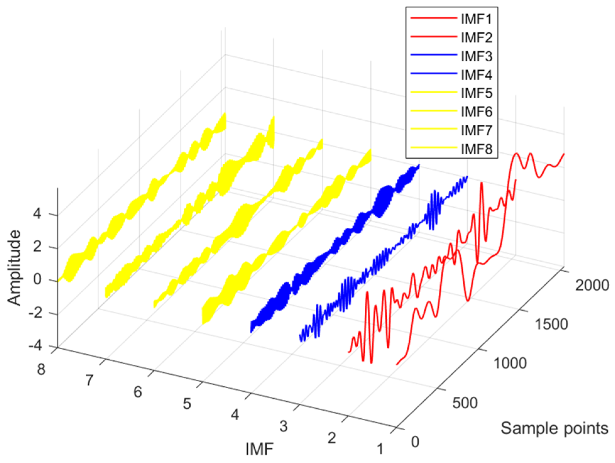
• SVMD adaptively decomposed SN into certain IMFs.
• The FuDE of each IMF was calculated.
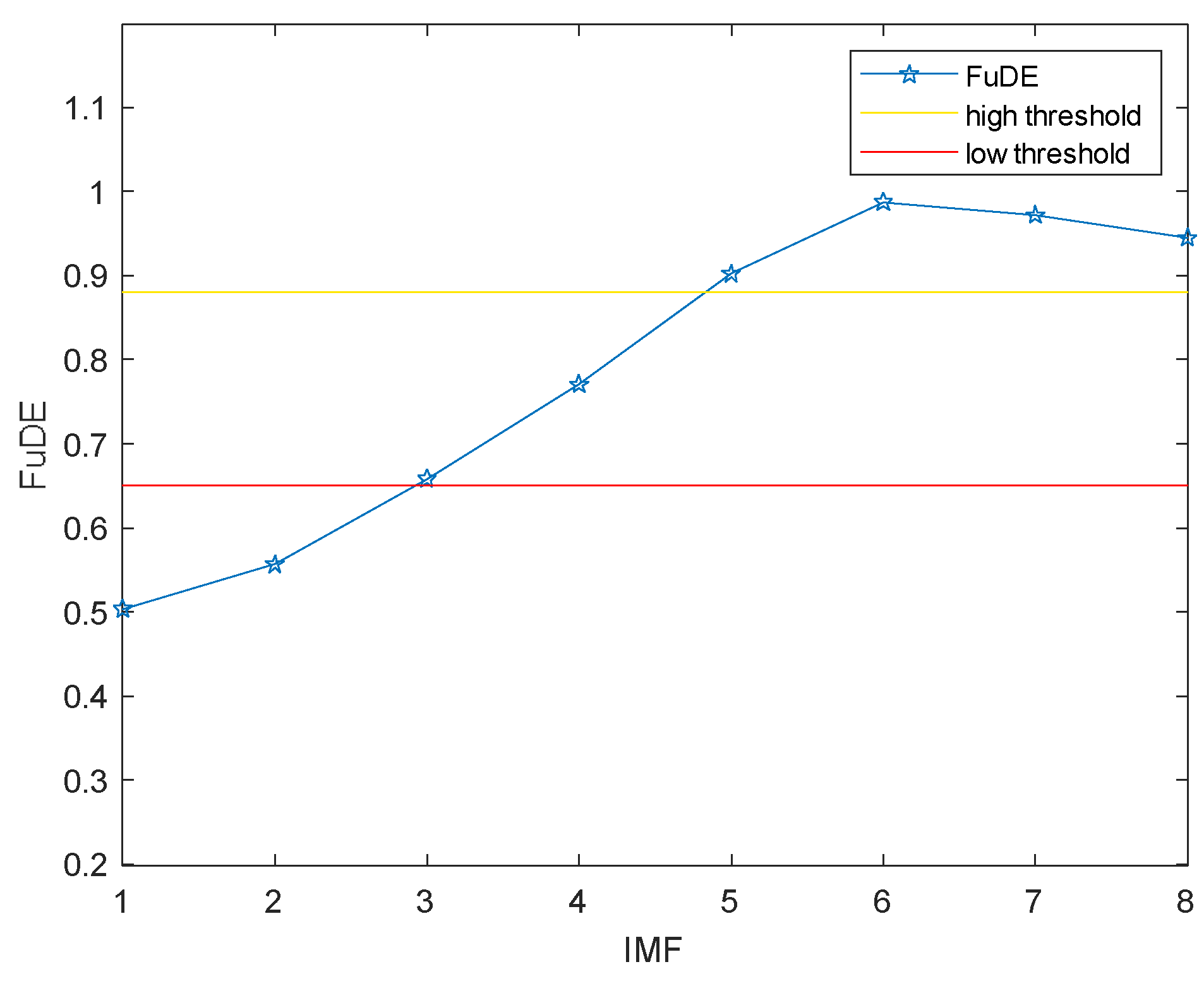
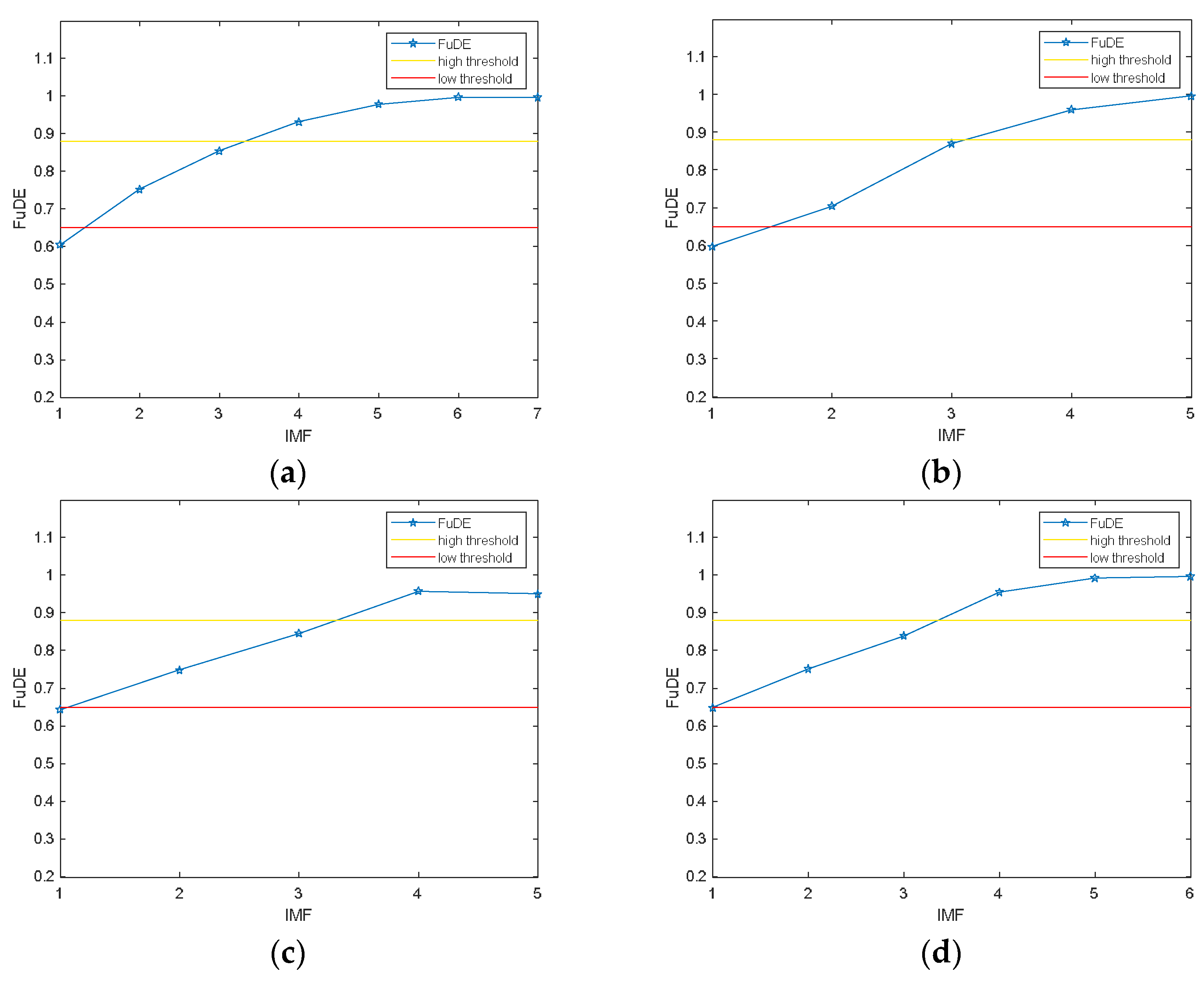
• According to the FuDE-based dual-threshold analysis, both high threshold (Hth) and low threshold (Lth) were obtained.
• The IMFs could be classified into three categories based on the high and low thresholds, including signal IMFs, noise–signal IMFs and noise IMFs.
• The denoised signal was obtained by reconstructing the signal IMFs and denoised noise–signal IMFs, and the noise IMFs were discarded.

4. Denoising Experiment for Simulation Signals

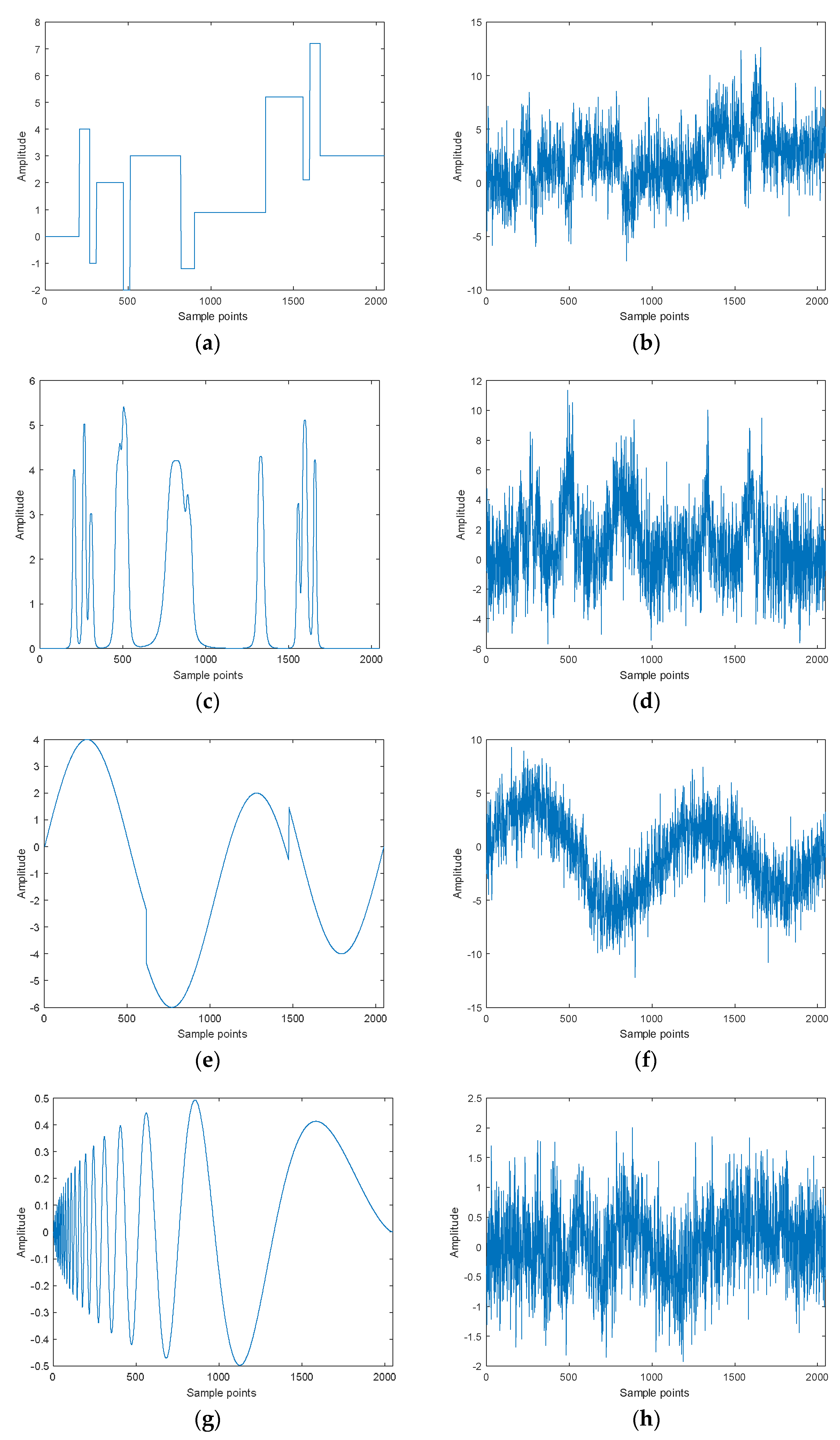
4.1. Four Types of Test Signals

There were four types of simulation signals chosen as classical examples for denoising, which were Blocks, Bumps, HeavySine and Doppler, and the length of the simulation signals was 2048 sample points [33]. We added white Gaussian noise to four test signals to obtain the noisy test signals with a −6 dB signal-to-noise ratio (SNR). Figure 2 shows the waveforms of the four test signals in the noiseless case and at the SNR of the −6 dB case.

4.2. Denoising Experiment of Test Signals

4.2.1. SVMD of Simulation Signals

To verify the effectiveness and feasibility of the proposed method, the SVMD-FuDE-WPD was applied to four test signals. Taking the Blocks signal as an example, the noisy Blocks (−6 dB) was decomposed using SVMD into eight IMFs. Figure 3 shows the decomposition results of the noisy Blocks. In Figure 3, the frequency increases with the increase in IMF order.

4.2.2. FuDE-Based Dual-Threshold Analysis and IMF Classification

The dual-threshold analysis was used to obtain the high and low thresholds. And signal IMFs, noise–signal IMFs and noise IMFs were determined using high and low thresholds. The FuDE of the four test signals was calculated with different SNRs, as shown in Figure 4. Further, Figure 5 shows the average FuDE of the four test signals. From Figure 5, the average FuDE of the four test signals tends to decrease with the increase in SNR. The decreasing trend of the FuDE is most obvious when the SNR increases from −5 dB to 0 dB, which decreases the FuDE from 0.9551 to 0.8811; with the increase in SNR, the FuDE becomes lower and gradually stabilizes at around 0.65.

Like [31], through FuDE-based dual-threshold analysis, 0.89 was identified as the high threshold since the FuDE decreased sharply from 0.9551 to 0.8811; 0.65 was determined as the low threshold due to the FuDE settling at 0.65. The high and low thresholds and FuDE of each IMF are shown in Figure 6. According to the FuDE-based dual-threshold analysis, the last four IMFs above the high threshold were determined as noise IMFs; the FuDE of the first two IMFs was lower than the low threshold; therefore, IMF1 and IMF2 were determined to be signal IMFs; the third and fourth IMFs, which were between the two thresholds, were noise–signal IMFs.

The result of the IMF classification for Blocks(−6 dB) is shown in Figure 7. As can be observed from Figure 7, the red IMFs were considered as signal IMFs to be saved; yellow IMFs were considered as noise IMFs to be discard; and the noise–signal IMFs in blue should be denoised via WPD.

4.2.3. Denoising and Reconstruction

After the IMF classification, the next step was to denoise the noise–signal IMF using WPD. The Meyer wavelet was selected for denoising, and the number of decomposition layers was three. Then, the signal IMF and denoised noise–signal IMF were reconstructed to obtain the denoised Blocks signal. The noiseless Blocks signal and denoised Blocks signal are shown in Figure 8. It depicts the difference in waveforms before and after denoising, and the waveform of the denoised signal is close to the noiseless signal, which reflects the feasibility of the proposed method.

4.3. Comparation of Denoising Methods

4.3.1. Evaluation Metrics

Aiming to evaluate the denoising effect quantitatively and intuitively, three metrics were selected for analysis, which were the SNR, root mean square error (RMS-E) and correlation coefficient (C-C). The SNR, RMS-E and C-C are defined as follows:

$$RMSE=\sqrt{\left[\frac{{\sum }_{i=1}^N{(f^{\prime }\left(i\right)-f\left(i\right))}^2}{N}\right]}$$

(20)

$$CC=\frac{{\sum }_{i=1}^N{f}^{\prime }\left(i\right)f\left(i\right)}{\sqrt{{\sum }_{i=1}^N{f}^{\prime 2}\left(i\right){\sum }_{i=1}^N{f}^2\left(i\right)}}$$

(21)

where $N$ represents the length of the signal; $f\left(i\right)$ and $f^{\prime }\left(i\right)$ are the ith original noiseless and denoised signal. A larger SNR and smaller RMS-E indicate less noise content in the signal, and a larger C-C denotes a higher similarity to the original noiseless signal. Thus, a larger SNR and C-C and a smaller RMS-E represent a better denoising effect.

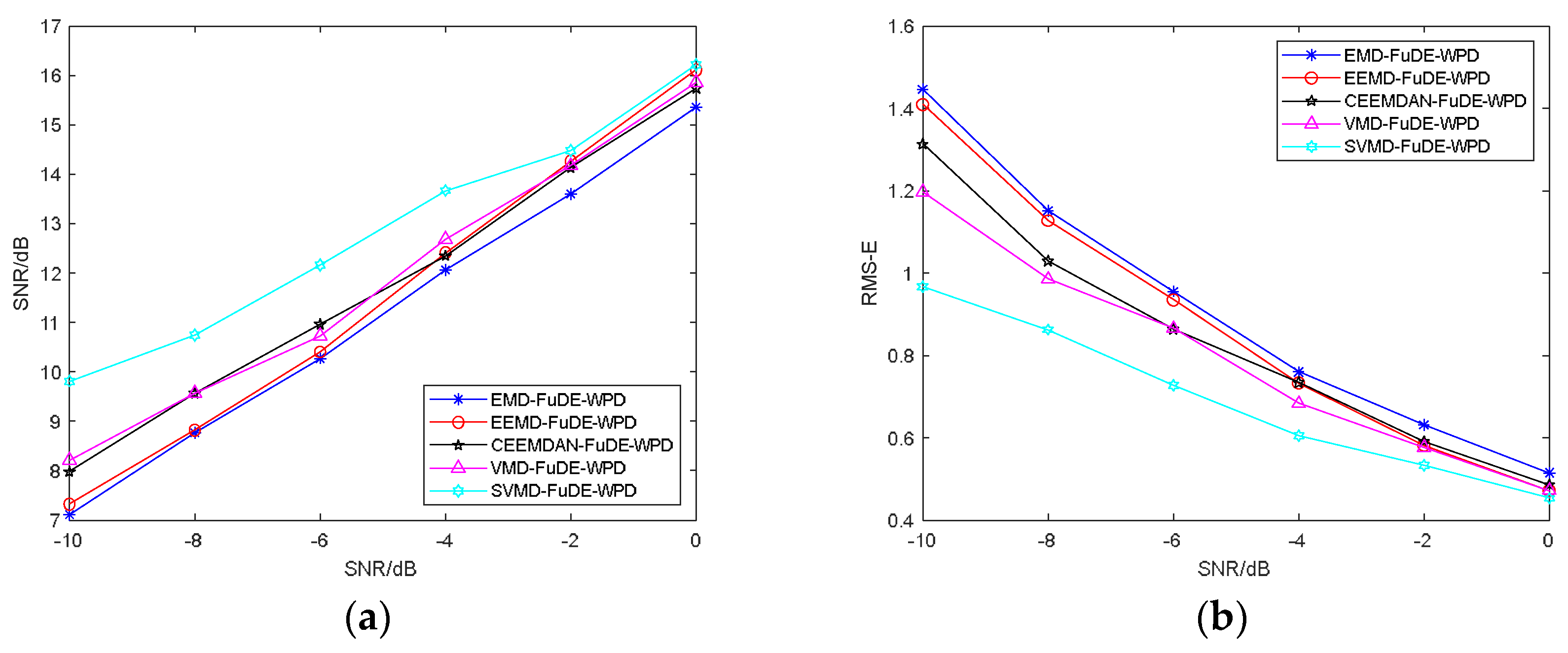
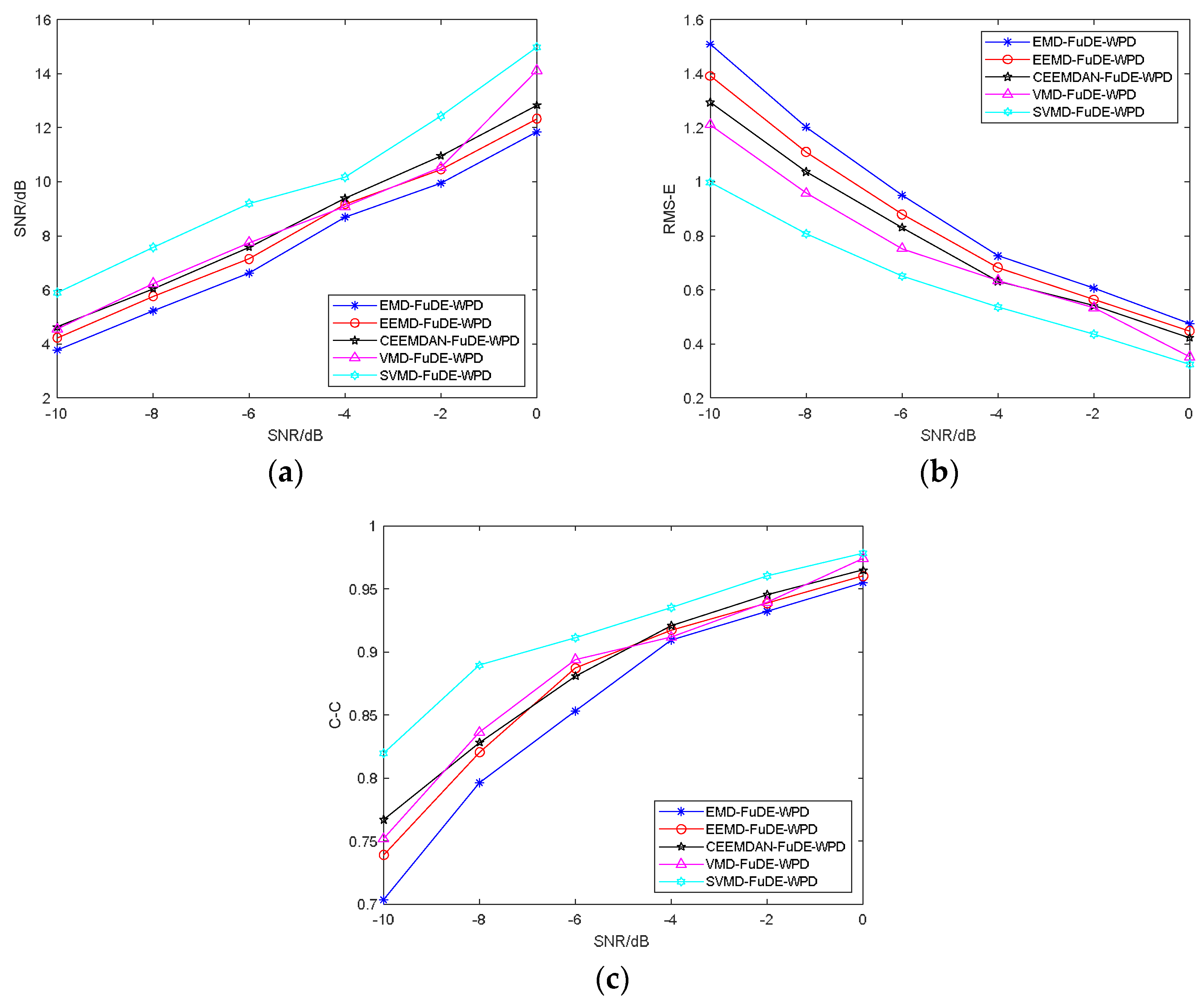
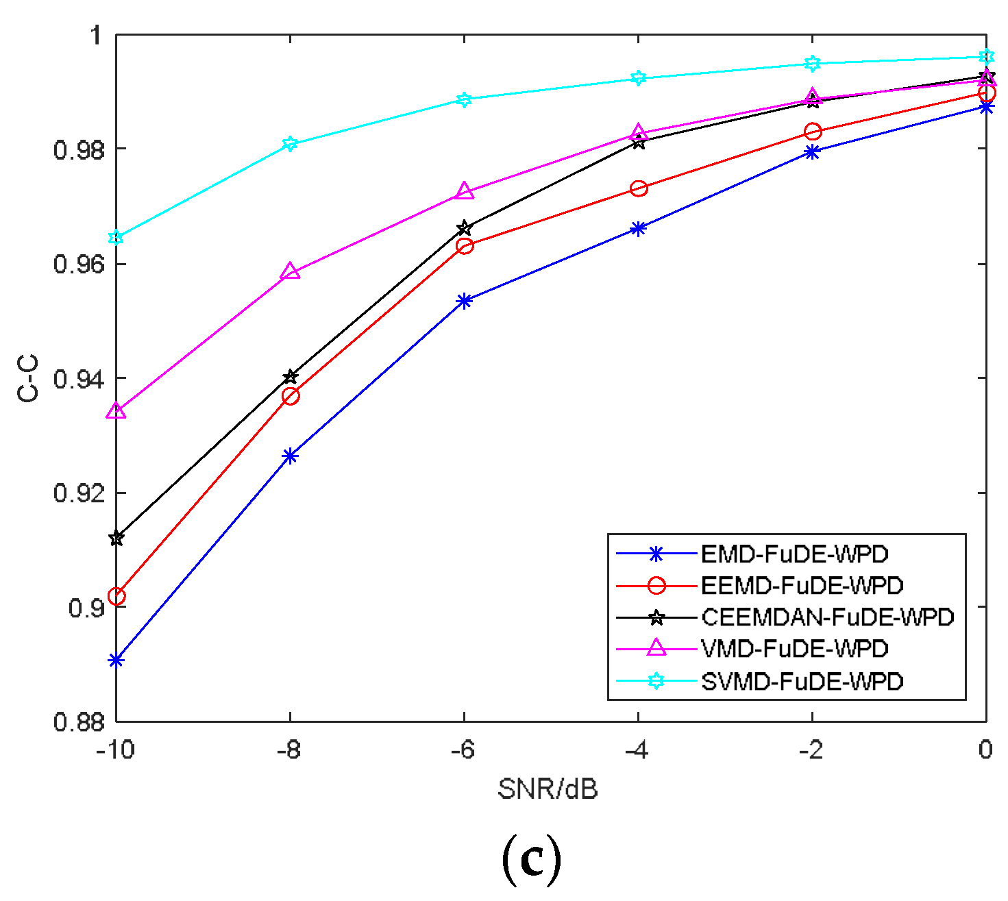
4.3.2. Comparative Analysis

To demonstrate the effectiveness of the proposed SVMD-FuDE-WPD method, different signal decomposition methods combined with the FuDE-based dual-threshold analysis and WPD were chosen as the comparison denoising methods, termed EMD-FuDE-WPD, EEMD-FuDE-WPD, CEEMDAN-FuDE-WPD and VMD-FuDE-WPD. Among them, the WPD denoising process of all five methods utilized Meyer wavelets and the number of decomposition layers was three. Moreover, the denoising experiments were performed on four test signals with different SNRs; these noisy signals were between −10 dB and 0 dB at 2 dB intervals.

To enhance the reliability of the experiments, the denoising experiments were repeated ten times for each type of signal, and the mean values of SNR, RMS-E and C-C were calculated for the five denoising methods for the different signals.

Table 1. Denoising result of Blocks across five methods.

SNR (dB)	Parameter	Denoising Methods
		EMD- FuDE-WPD	EEMD-FuDE-WPD	CEEMDAN-FuDE-WPD	VMD-FuDE-WPD	Proposed
−10	SNR (dB)	7.1123	7.3263	7.9787	8.2092	9.8129
	RMS-E-	1.4452	1.4090	1.3131	1.1964	0.9669
	C-C	0.7951	0.8161	0.8345	0.8347	0.8775
−8	SNR (dB)	8.7669	8.8213	9.5679	9.5642	10.7419
	RMS-E	1.1512	1.1267	1.0290	0.9847	0.8622
	C-C	0.8608	0.8651	0.8822	0.8794	0.9019
−6	SNR (dB)	10.2715	10.4009	10.9614	10.7204	12.1555
	RMS-E	0.9554	0.9346	0.8634	0.8651	0.72627
	C-C	0.9006	0.9016	0.9164	0.9051	0.9317
−4	SNR (dB)	12.0612	12.4051	12.3482	12.6794	13.6665
	RMS-E	0.7595	0.7328	0.7335	0.6829	0.6046
	C-C	0.9318	0.9396	0.9359	0.9384	0.9522
−2	SNR (dB)	13.5964	14.2625	14.1302	14.1702	14.4824
	RMS-E	0.6311	0.5819	0.5913	0.5770	0.5322
	C-C	0.9520	0.9588	0.9567	0.9373	0.9631
0	SNR (dB)	15.3607	16.1055	15.7362	15.8557	16.2097
	RMS-E	0.5149	0.4716	0.4857	0.4717	0.4529
	C-C	0.9676	0.9726	0.9581	0.9714	0.9738

,

Table 2. Denoising result of Bumps across five methods.

SNR (dB)	Parameters	Denoising Methods
		EMD- FuDE-WPD	EEMD-FuDE-WPD	CEEMDAN-FuDE-WPD	VMD-FuDE-WPD	Proposed
−10	SNR (dB)	3.7562	4.2255	4.6239	4.5349	5.8977
	RMS-E	1.5080	1.3910	1.2937	1.2107	0.9976
	C-C	0.7035	0.7389	0.7668	0.7516	0.8194
−8	SNR (dB)	5.2223	5.7629	6.0370	6.2175	7.5599
	RMS-E	1.2024	1.1100	1.0366	0.9570	0.8072
	C-C	0.7963	0.8204	0.8281	0.8361	0.8893
−6	SNR (dB)	6.6256	7.1416	7.5747	7.7470	9.1989
	RMS-E	0.9502	0.8791	0.8301	0.7525	0.6495
	C-C	0.8530	0.8869	0.8808	0.8937	0.9110
−4	SNR (dB)	8.6903	9.1641	9.3790	9.0854	10.1697
	RMS-E	0.7249	0.6824	0.6305	0.6344	0.5358
	C-C	0.9093	0.9174	0.9208	0.9115	0.9353
−2	SNR (dB)	9.9321	10.4520	10.9616	10.5184	12.4269
	RMS-E	0.6063	0.5637	0.5403	0.5329	0.4360
	C-C	0.9322	0.9385	0.9452	0.9393	0.9603
0	SNR (dB)	11.8321	12.3313	12.8301	14.1153	14.9826
	RMS-E	0.4732	0.4477	0.4226	0.3519	0.3230
	C-C	0.9550	0.9601	0.9648	0.9741	0.9780

,

Table 3. Denoising result of HeavySine across five methods.

SNR (dB)	Parameters	Denoising Methods
		EMD- FuDE-WPD	EEMD-FuDE-WPD	CEEMDAN-FuDE-WPD	VMD-FuDE-WPD	Proposed
−10	SNR (dB)	7.1206	7.6017	8.3059	9.2277	11.9972
	RMS-E	1.4862	1.4138	1.2932	1.1304	0.8092
	C-C	0.8907	0.9019	0.9120	0.9340	0.9646
−8	SNR (dB)	8.7535	9.4141	9.6216	11.1875	14.6590
	RMS-E	1.1932	1.1116	1.0725	0.8899	0.5843
	C-C	0.9265	0.9369	0.9402	0.9584	0.9809
−6	SNR (dB)	10.7013	11.4311	12.1106	12.9648	16.6854
	RMS-E	0.9351	0.8554	0.8033	0.7098	0.4550
	C-C	0.9535	0.9631	0.9662	0.9725	0.9886
−4	SNR (dB)	12.8621	13.0554	14.7153	14.9012	18.4936
	RMS-E	0.7186	0.6975	0.5821	0.5641	0.3672
	C-C	0.9661	0.9731	0.9813	0.9826	0.9924
−2	SNR (dB)	14.2346	15.0312	16.6148	16.7928	20.2769
	RMS-E	0.6128	0.5544	0.4604	0.4476	0.2999
	C-C	0.9795	0.9830	0.9883	0.9888	0.9950
0	SNR (dB)	16.3358	17.2349	18.7690	18.3044	21.2527
	RMS-E	0.4771	0.4257	0.3585	0.3777	0.2598
	C-C	0.9874	0.9898	0.9928	0.9921	0.9962

and

Table 4. Denoising result of Doppler across five methods.

SNR (dB)	Parameters	Denoising Methods
		EMD- FuDE-WPD	EEMD-FuDE-WPD	CEEMDAN-FuDE-WPD	VMD-FuDE-WPD	Proposed
−10	SNR (dB)	1.4928	1.6554	2.0722	2.2558	3.0188
	RMS-E	0.4347	0.4223	0.3678	0.3410	0.3007
	C-C	0.5335	0.5562	0.6103	0.6333	0.6951
−8	SNR (dB)	2.1155	2.6804	2.7758	3.0444	4.1249
	RMS-E	0.3476	0.3255	0.3001	0.2796	0.2494
	C-C	0.6181	0.6727	0.6825	0.7088	0.7791
−6	SNR (dB)	3.1346	3.5160	3.8485	4.1854	4.5290
	RMS-E	0.2822	0.2627	0.2437	0.2173	0.2191
	C-C	0.7083	0.7423	0.7609	0.7315	0.8001
−4	SNR (dB)	4.2189	4.9282	5.1783	5.4913	6.3261
	RMS-E	0.2225	0.2011	0.1906	0.1774	0.1627
	C-C	0.7854	0.8215	0.8319	0.8440	0.8714
−2	SNR (dB)	6.3355	6.4252	6.3921	7.0159	8.7687
	RMS-E	0.1589	0.1599	0.1592	0.1406	0.1164
	C-C	0.8743	0.8757	0.8757	0.8853	0.9270
0	SNR (dB)	8.0902	7.8850	7.8137	8.6208	10.1565
	RMS-E	0.1258	0.1288	0.1288	0.1120	0.0949
	C-C	0.9179	0.9115	0.9127	0.9314	0.9495

illustrate the denoising results of the five denoising methods for the four types of signals. As shown in Table 1, Table 2, Table 3 and Table 4, for the proposed method, the SNR improvement is stable for Blocks and HeavySine signals, which is above 16 dB for different SNR conditions; for the Bumps signal and Doppler signal, the improvement of SNR is approximately 10 dB, which is lower than that of the other two signals; compared with other denoising methods, SVMD-FuDE-WPD generally has the highest SNR improvement value.

Additionally, for non-linear signals such as Blocks, Bumps, HeavySine and Doppler, the denoising effect of EMD-FuDE-WPD is generally inferior to the other four denoising methods, while the SVMD-FuDE-WPD is substantially superior to the first four denoising methods due to it having the highest SNR and C-C, and the lowest RMS-E. In summary, the proposed method has the best denoising performance.

Figure 9, Figure 10, Figure 11 and Figure 12 demonstrate the evaluation metrics comparisons of the four test signals across the five methods. From Figure 9, Figure 10, Figure 11 and Figure 12, it can be concluded that the proposed method has the highest SNR and C-C, and the lowest RMS-E for all signals, which means that the proposed method has the most brilliant denoising performance.

5. Experiment and Analysis of SN

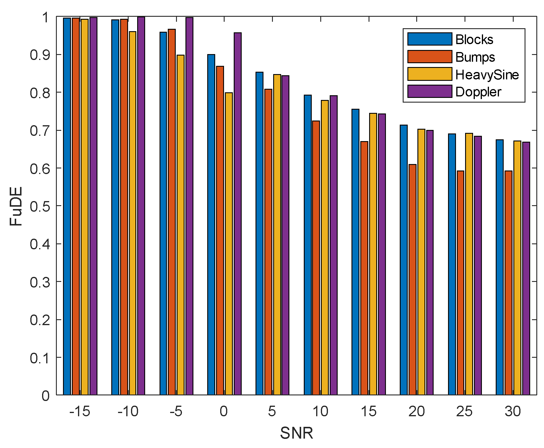
5.1. Four Types of SNs and Evaluation Criterion

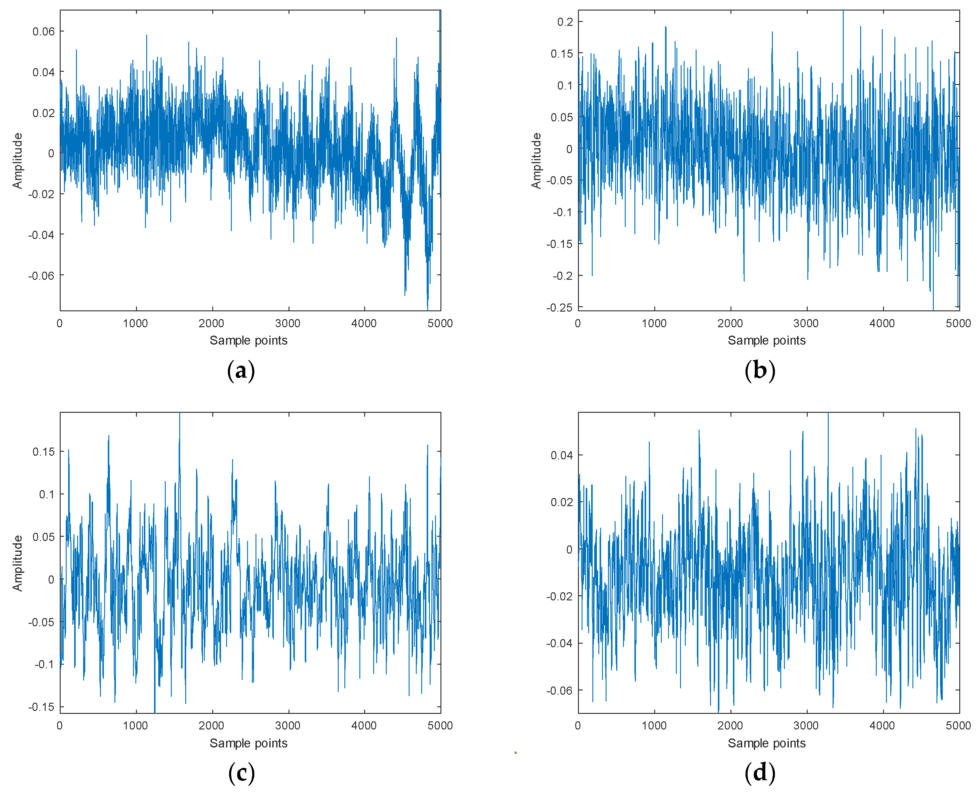
5.1.1. Four Types of SNs

Aiming to verify the validity of the proposed method SVMD-FuDE-WPD, four types of SNs were selected, which were from the National Park Service [34]. These four SNs contained different levels of marine environment noise and equipment noise, namely SN-1, SN-2, SN-3 and SN-4; Figure 13 displays the waveform of the four types of SNs, sampled at length $N=5000$.

Figure 14 shows the frequency spectrogram of the four types of SNs. As shown in Figure 14, for the four types of SNs, the energy above 15 kHz is significantly lower than the energy below 15 kHz; the spectrograms of SN-1 and SN-2 are semblable; and the spectrograms of SN-3 and SN-4 are also similar, except for between 84 s and 89 s.

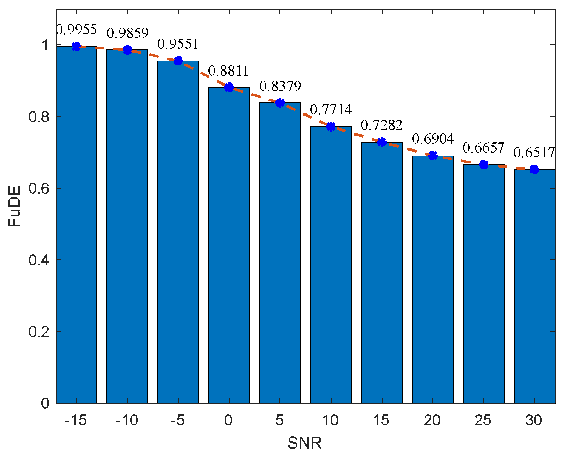
5.1.2. Evaluation Criterion

In the absence of noiseless signals for comparison, to illustrate the validity of the proposed denoising method, an evaluation criterion relying on attractor trajectory was proposed. In the realm of chaos theory, attractor trajectory is a widely recognized concept. Attractor trajectories exhibit an extreme sensitivity to initial conditions, resulting in vastly different shapes when even the slightest change in the initial conditions occurs. In terms of SN, noiseless signals tend to yield smooth and regular attractor trajectories, whereas noisy signals are characterized by their disordered and irregular attractor trajectories.

Due to the SN having chaotic characteristics [35], we introduced two chaotic feature parameters based on entropy, which were DE and PE, to further demonstrate the effectiveness of the proposed method [36]. The DE and PE could exactly measure the complicacy of the time series; the smaller the value of the DE and PE, the better the denoising effect. Therefore, the validity of the denoising method could be verified by comparing the attractor trajectories, DE and PE before and after the SN denoising.

5.2. Denoising Experiment of SN

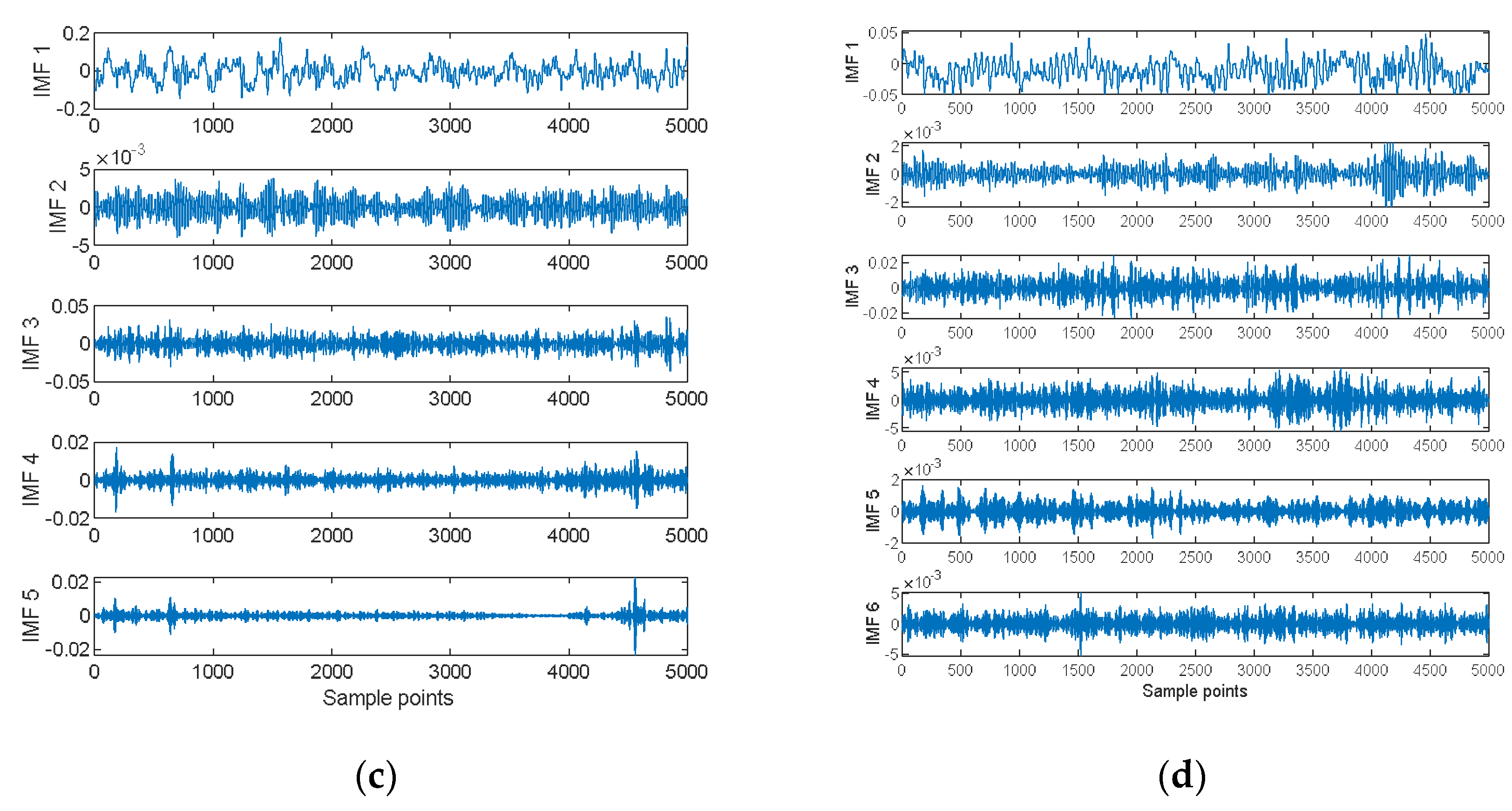
5.2.1. Decomposed SN via SVMD

Four SNs were decomposed into several IMFs via SVMD. The decomposition results of the SN are exhibited in Figure 15. Taking SN-1 as an example, SVMD precisely decomposed SN-1 into seven IMFs. It can be seen that the frequency increased with the number of IMF orders.

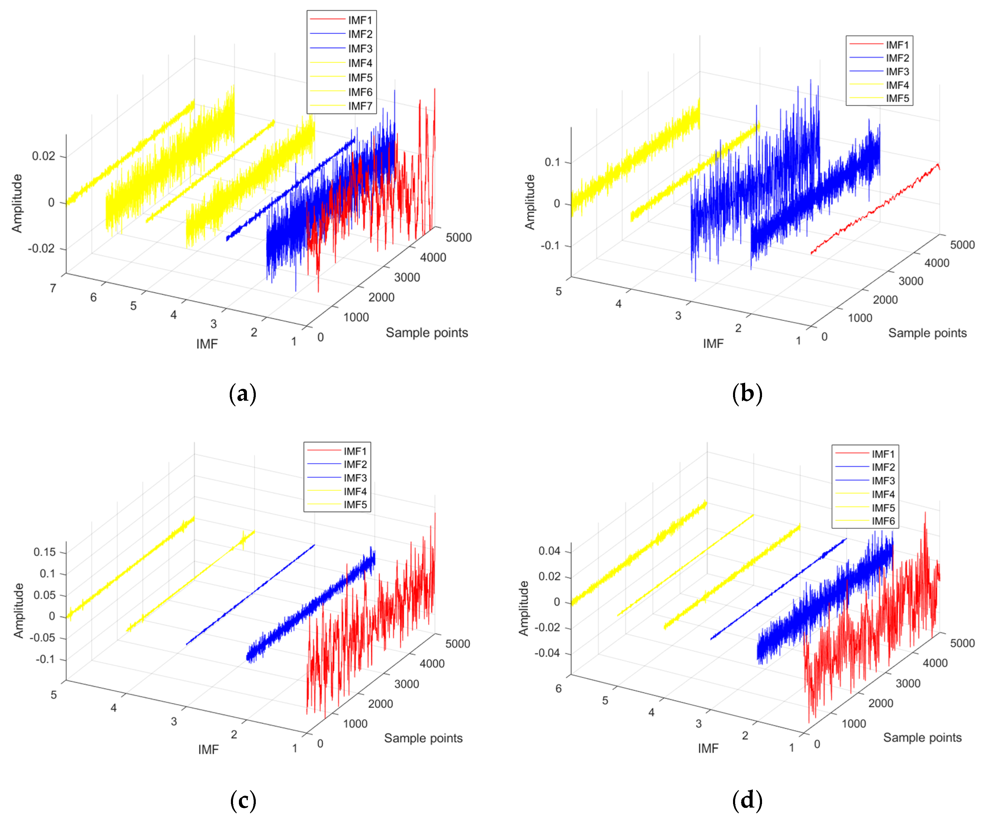
5.2.2. Classification and Reconstruction of IMF

The high and low thresholds were obtained separately according to the FuDE-based dual-thresholds analysis. And signal IMFs, noise–signal IMFs and noise IMFs could be classified using the dual-thresholds analysis. Figure 16 displays the dual-thresholds and FuDE of each IMF for the four SNs. As shown in Figure 16, the IMFs of the four SNs are divided into three categories. Taking SN-1 as an example, the FuDE of IMF1 is under the low threshold, the FuDE of IMF3 and IMF4 are between the high and low thresholds, and the FuDE of the remaining four IMFs are above the high threshold. In conclusion, IMF1 is regarded as signal IMFs, IMF2 and IMF3 are regarded as noise–signal IMFs and the remainder of the IMFs are all noise IMFs.

Figure 17 shows the classification results of the four SNs. As shown in Figure 17, the signal IMFs in red would be saved, the signal-noise IMFs in blue are supposed to be denoised via WPD, and the rest of the IMFs in yellow are noise IMFs that should be discarded. Finally, the signal IMFs and denoised noise–signal IMFs were reconstructed to obtain the denoising SN signal.

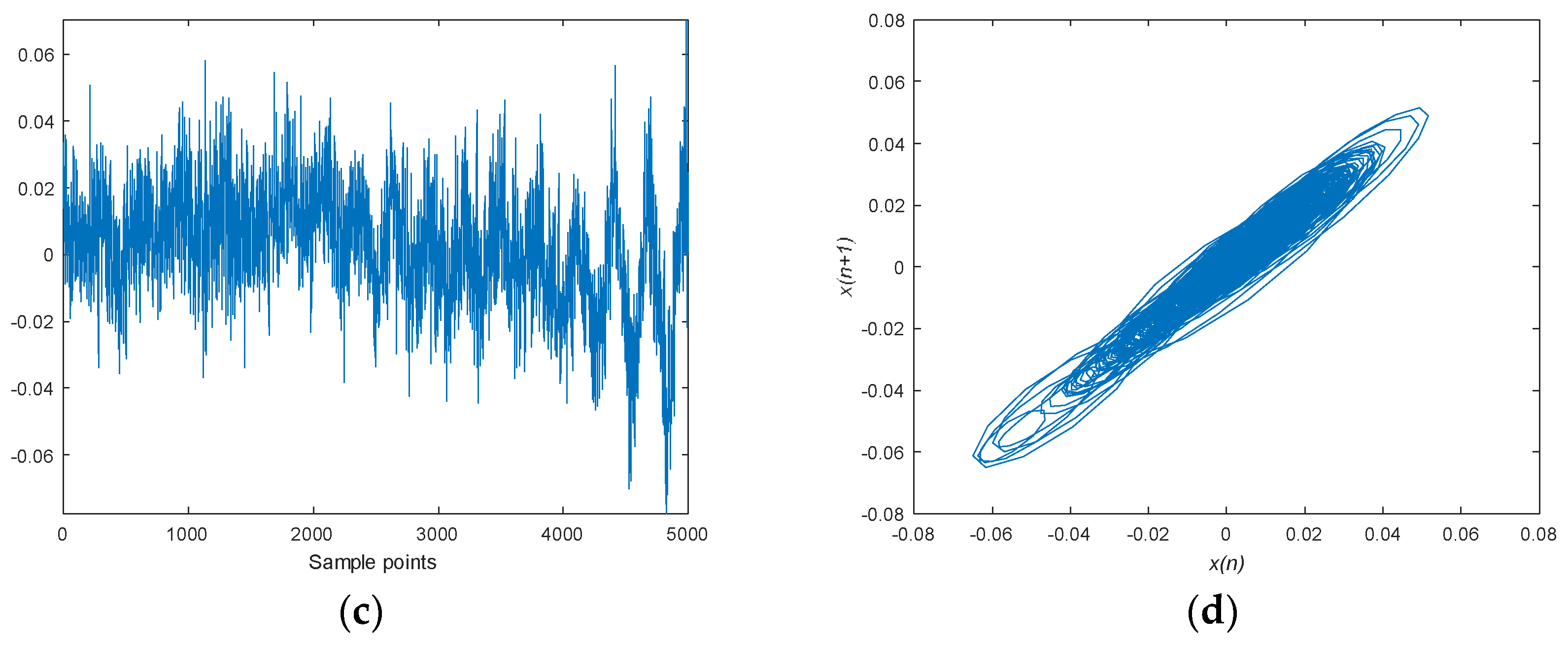
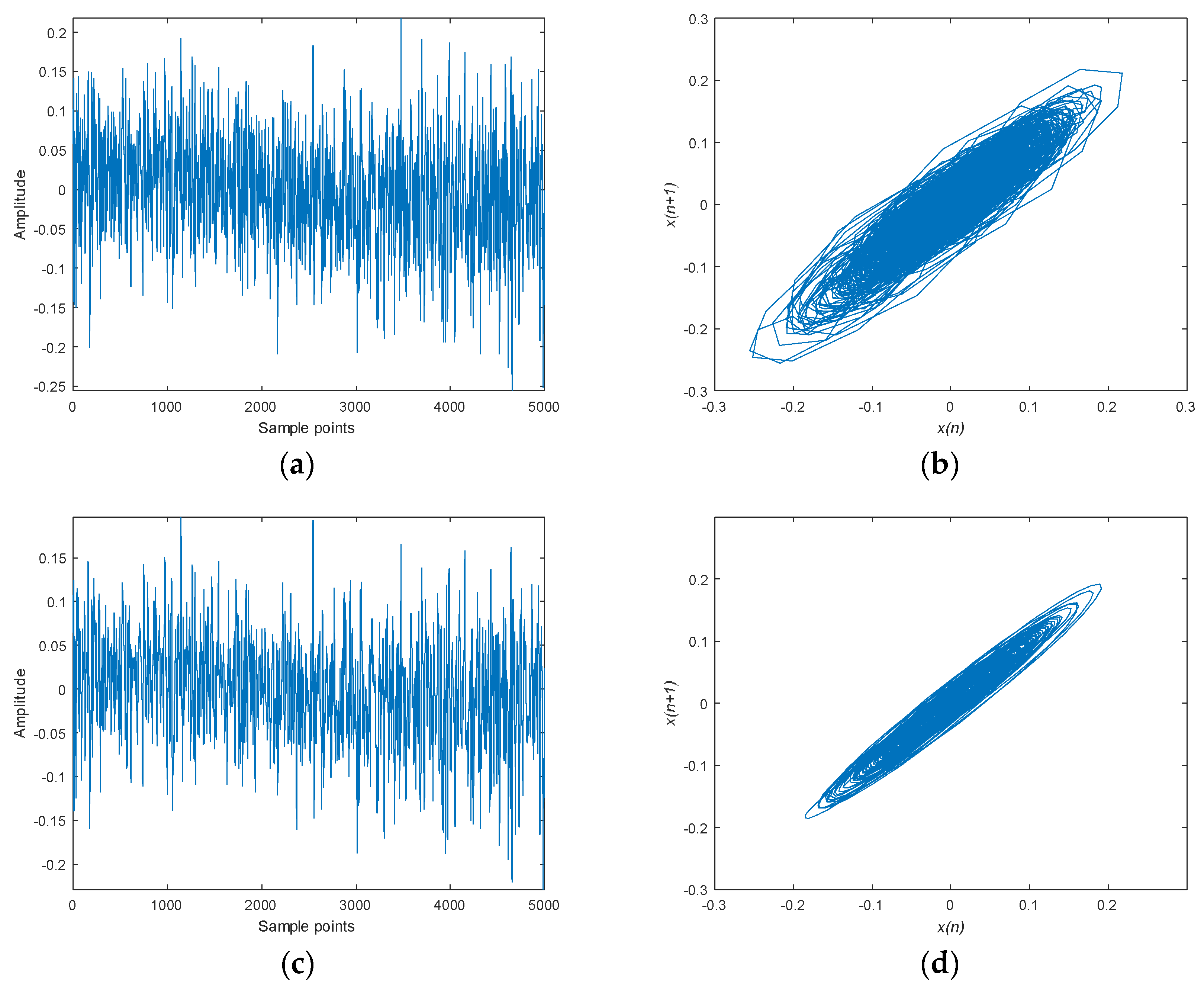
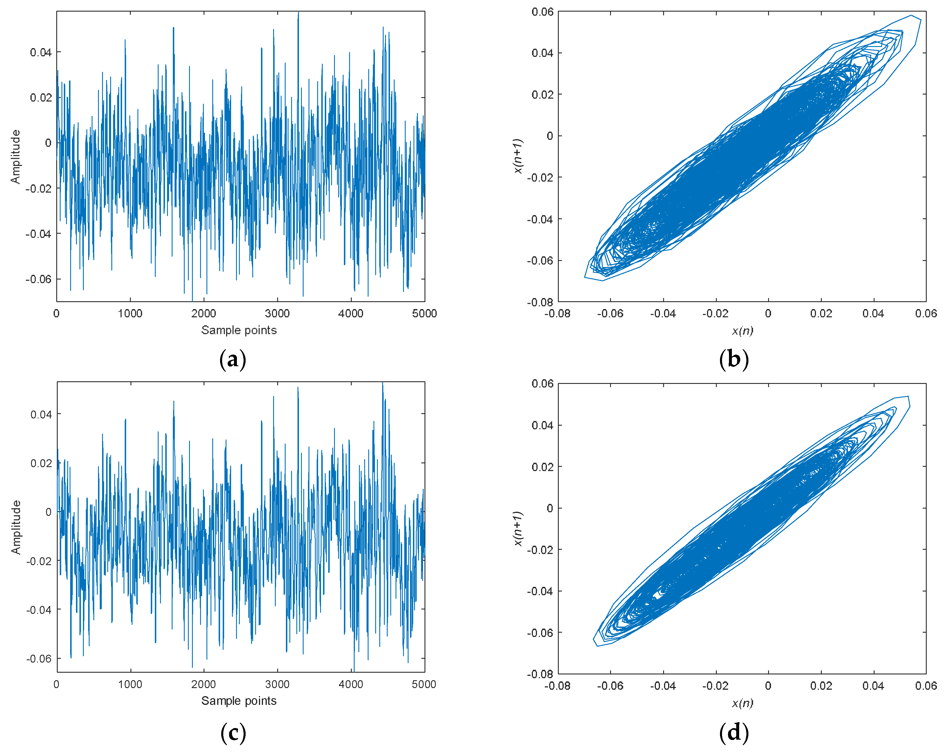
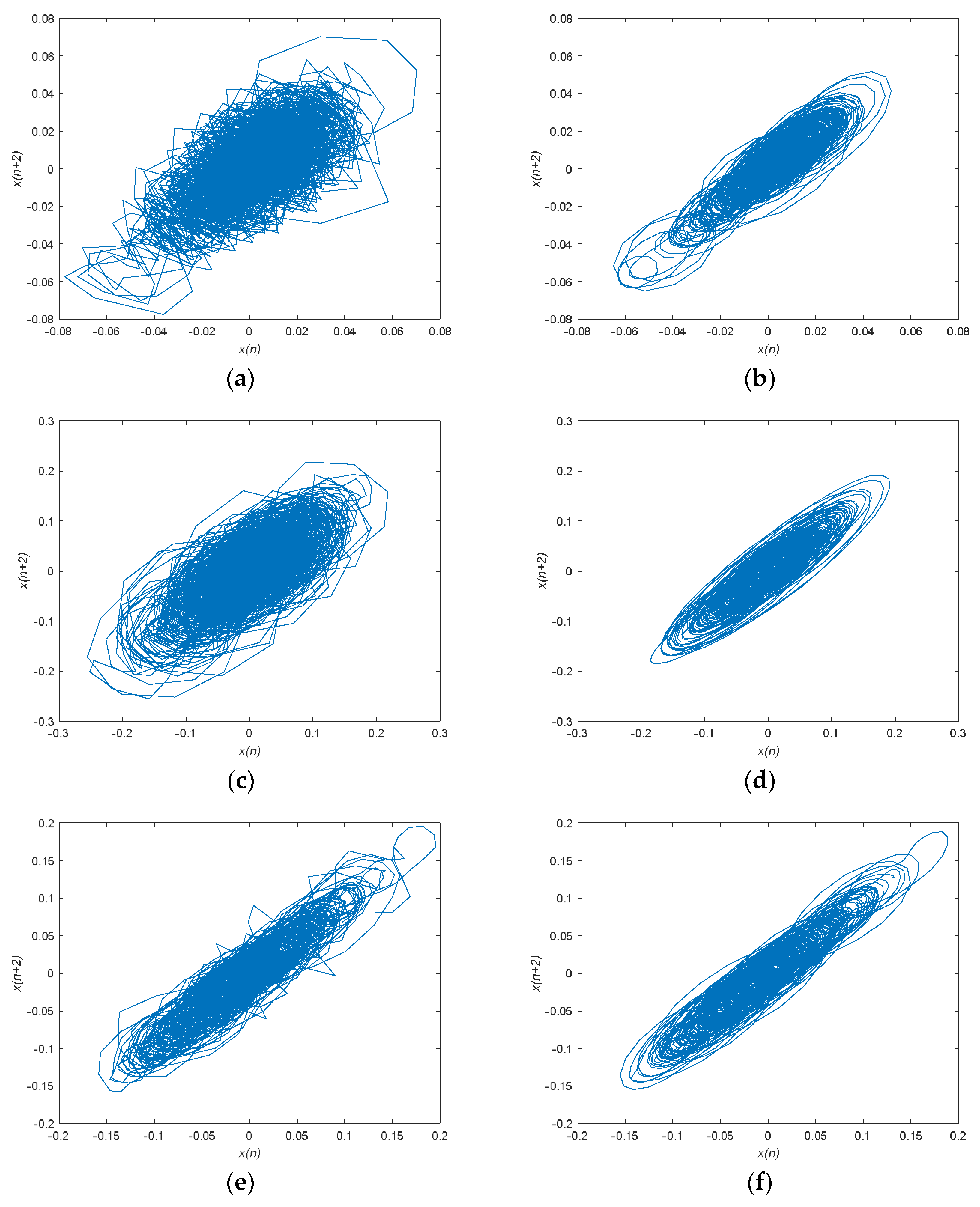
5.2.3. Denoising Result and Analysis

Figure 18, Figure 19, Figure 20 and Figure 21 display the waveform and attractor trajectories for the original and denoised SN. The attractor trajectories are plotted in the interval on one sample point to prevent similar values among neighboring amplitudes. Therefore, the horizontal axis represents the amplitude of x(n) and the vertical axis represents the amplitude of x(n + 1), where n represents the sample point.

As can be seen from Figure 18, Figure 19, Figure 20 and Figure 21, the waveforms of the denoised SN became cleaner, representing how the marine environment noise of the SN was well suppressed; moreover, the attractor trajectories of the denoised SN became more regular and smooth. The experiments result shows that the proposed method performed excellently at denoising SN.

To further verify the denoising effectiveness of the proposed method for SN, we have plotted delay x(n + d) against x(n) with different d. Figure 22 and Figure 23 show the attractor trajectories of delay x(n + d) against x(n) with different d for the original and denoised SNs, where we only demonstrate x(n + 2) and x(n + 3). As shown in Figure 22 and Figure 23, the attractor trajectories of the denoised SNs are became more regular and smooth, and the results are similar to x(n + 1) against x(n), which manifests that the proposed SVMD-FuDE-WPD denoising method in this paper can effectively eliminate SN.

In order to quantitatively analyze the effect of the proposed denoising method, the DE and PE of the above four types of SNs before and after denoising were calculated separately.

Table 5. Comparison of feature parameters before and after denoising of SN.

SN Signal	Status	DE	PE
SN-1	Original	0.8601	1.6513
	Denoised	0.7179	1.0502
SN-2	Original	0.8030	1.4610
	Denoised	0.6979	1.0403
SN-3	Original	0.6981	1.3301
	Denoised	0.6705	1.1163
SN-4	Original	0.7450	1.3877
	Denoised	0.7124	1.1892

demonstrates the DE and PE of the original and denoised SN. As shown in Table 5, denoised SN has a smaller DE and PE, which shows the validity of the proposed method.

6. Conclusions

A novel SN denoising method is proposed based on the combination of SVMD with FuDE-based dual-threshold analysis and WPD. The simulation and measured SN experiments demonstrate the validity of the proposed denoising method. The advantages and conclusions of SVMD-FuDE-WPD are as follows.

(1)

SVMD-FuDE-WPD was proposed as the denoising method for SN; SVMD can resolve the parameter selection problem of VMD and suppresses the mode mixing of EMD, and the FuDE-based dual-threshold analysis precisely classifies IMF into three categories.

(2)

Compared with EMD-FuDE-WPD, EEMD-FuDE-WPD, CEEMDAN-FuDE-WPD and VMD-FuDE-WPD, the proposed method has the lowest RMS-E as well as the highest SNR and C-C, which shows a better denoising performance.

(3)

The SVMD-FuDE-WPD method leads to much smoother and more regular attractor trajectories, more distinct waveforms of SN, and lower DE and PE values, which prove that the proposed method performs effectively at denoising SN.

The proposed SVMD-FuDE-WPD denoising method can effectively suppress SN, which contributes to the feature extraction and classification of SN, and further promotes the detection and tracking of underwater acoustic signals. However, we only applied the proposed method to SN from single database, and the denoising effect of many more SNs in different databases still remains to be verified. In the future, we will investigate the application of the proposed denoising method on other underwater acoustic signals to further verify the effectiveness of the proposed method.

References

1. Niu, F.; Hui, J.; Zhao, A.; Cheng, Y.; Chen, Y. Application of SN-EMD in Mode Feature Extraction of Ship Radiated Noise. Math. Probl. Eng. 2018, 20, 2184612. [Google Scholar] [CrossRef]
2. Siddagangaiah, S.; Li, Y.; Guo, X.; Yang, K. On the dynamics of ocean ambient noise: Two decades later. Chaos 2015, 25, 103117. [Google Scholar] [CrossRef] [PubMed]
3. Tucker, J.D.; Azimi-Sadjadi, M.R. Coherence-based underwater target detection from multiple disparatesonar platforms. IEEE J. Ocean Eng. 2011, 36, 37–51. [Google Scholar] [CrossRef]
4. Jiang, J.; Shi, T.; Huang, M.; Xiao, Z. Multi-Scale Spectral Feature Extraction for Underwater Acoustic Target Recognition. Measurement 2020, 166, 108227. [Google Scholar] [CrossRef]
5. Baskar, V.V.; Rajendran, V.; Logashanmugam, E. Study of different denoising methods for underwater acoustic signal. J. Mar. Sci. Technol. 2015, 23, 414–419. [Google Scholar]
6. Siddagangaiah, S.; Li, Y.; Guo, X.; Chen, X.; Zhang, Q.; Yang, K.; Yang, Y. A Complexity-Based Approach for the Detection of Weak Signals in Ocean Ambient Noise. Entropy 2016, 18, 101. [Google Scholar] [CrossRef]
7. Cawley, R.; Hsu, G.H. Local-geometric project ion method for noise reduction in chaotic maps and flows. Phys. Rev. A 1992, 46, 3057–3082. [Google Scholar] [CrossRef]
8. Buchris, Y.; Amar, A.; Benesty, J.; Cohen, I. Incoherent synthesis of sparse arrays for frequency-invariant beamforming. IEEE/ACM Trans. Audio Speech Lang. Process. 2018, 27, 482–495. [Google Scholar] [CrossRef]
9. Zhao, X.; Ye, B. Selection of effective singular values using difference spectrum and its application to fault diagnosis of headstock. Mech. Syst. Signal Process. 2011, 25, 1617–1631. [Google Scholar] [CrossRef]
10. Li, Y.; Tang, B.; Geng, B.; Jiao, S. Fractional Order Fuzzy Dispersion Entropy and Its Application in Bearing Fault Diagnosis. Fractal Fract. 2022, 6, 544. [Google Scholar] [CrossRef]
11. Li, Y.; Jiao, S.; Geng, B. Refined composite multiscale fluctuation-based dispersion Lempel–Ziv complexity for signal analysis. ISA Trans. 2023, 133, 273–284. [Google Scholar] [CrossRef] [PubMed]
12. Li, Y.; Geng, B.; Tang, B. Simplified coded dispersion entropy: A nonlinear metric for signal analysis. Nonlinear Dyn. 2023, 111, 9327–9344. [Google Scholar] [CrossRef]
13. Huang, N.E.; Shen, Z.; Long, S.R.; Wu, M.C.; Shih, H.H.; Zheng, Q.; Yen, N.-C.; Tung, C.C.; Liu, H.H. The empirical mode decomposition and the Hilbert spectrum for nonlinear and non-stationary time series analysis. Proc. Math. Phys. Eng. Sci. 1998, 454, 903–995. [Google Scholar] [CrossRef]
14. Boudraa, A.O.; Cexus, J.C. EMD-Based signal filtering. IEEE Trans. Instrum. Meas. 2007, 56, 2196–2202. [Google Scholar] [CrossRef]
15. Kopsinis, Y.; McLaughlin, S. Development of EMD-based denoising methods inspired by wavelet thresholding. IEEE Trans. Signal Process. 2009, 57, 13511362. [Google Scholar] [CrossRef]
16. Torres, M.E.; Colominas, M.A.; Schlotthauer, G.; Flandrin, P. A complete ensemble empirical mode decomposition with adaptive noise. In Proceedings of the 2011 IEEE International Conference on Acoustics, Speech and Signal (ICASSP), Prague, Czech Republic, 22–27 May 2011; pp. 4144–4147. [Google Scholar]
17. Dragomiretskiy, K.; Zosso, D. Variational Mode Decomposition. IEEE Trans. Signal 2014, 62, 531–544. [Google Scholar] [CrossRef]
18. Yang, H.; Li, Y.A.; Li, G.H. Noise reduction method of ship radiated noise with ensemble empirical mode decomposition of adaptive noise. Noise Control Eng. J. 2016, 64, 230–242. [Google Scholar]
19. Li, Y.; Wang, L. A novel noise reduction technique for underwater acoustic signals based on complete ensemble empirical mode decomposition with adaptive noise, minimum mean square variance criterion and least mean square adaptive filter. Def. Technol. 2020, 16, 543–554. [Google Scholar] [CrossRef]
20. Yan, H.; Xu, T.; Wang, P.; Zhang, L.; Hu, H.; Bai, Y. MEMS Hydrophone Signal Denoising and Baseline Drift Removal Algorithm Based on Parameter-Optimized Variational Mode Decomposition and Correlation Coefficient. Sensors 2019, 19, 4622. [Google Scholar] [CrossRef] [PubMed]
21. Nazari, M.; Sakhaei, S.M. Successive Variational Mode Decomposition. Signal Process. 2020, 174, 107610. [Google Scholar] [CrossRef]
22. Li, Y.; Tang, B.; Jiao, S. SO-slope entropy coupled with SVMD: A novel adaptive feature extraction method for ship-radiated noise. Ocean Eng. 2023, 280, 114677. [Google Scholar] [CrossRef]
23. Guo, Y.; Yang, Y.; Jiang, S.; Jin, X.; Wei, Y. Rolling Bearing Fault Diagnosis Based on Successive Variational Mode Decomposition and the EP Index. Sensors 2022, 22, 3889. [Google Scholar] [CrossRef] [PubMed]
24. Zhang, L.; Zhang, Y.; Li, G. Fault-Diagnosis Method for Rotating Machinery Based on SVMD Entropy and Machine Learning. Algorithms 2023, 16, 304. [Google Scholar] [CrossRef]
25. Wu, X.; Zhang, T.; Zhang, L.; Qiao, L. Epileptic seizure prediction using successive variational mode decomposition and transformers deep learning network. Front. Neurosci. 2022, 16, 982541. [Google Scholar] [CrossRef] [PubMed]
26. Vashishtha, G.; Chauhan, S.; Singh, M.; Kumarn, R. Bearing defect identification by swarm decomposition considering permutation entropy measure and opposition-based slime mould algorithm. Measurement 2021, 178, 109389. [Google Scholar] [CrossRef]
27. Vashishtha, G.; Chauhan, S.; Yadav, N.; Yadav, N.; Kumar, N.; Kumar, R. A two-level adaptive chirp mode decomposition and tangent entropy in estimation of single-valued neutrosophic cross-entropy for detecting impeller defects in centrifugal pump. Appl. Acoust. 2022, 197, 108905. [Google Scholar] [CrossRef]
28. Figlus, T.; Gnap, J.; Skrúcaný, T.; Šarkan, B.; Stoklosa, J. The use of denoising and analysis of the acoustic signal entropy in diagnosing engine valve clearance. Entropy 2016, 18, 253. [Google Scholar] [CrossRef]
29. Li, G.; Yang, Z.; Yang, H. Noise Reduction Method of Underwater Acoustic Signals Based on Uniform Phase Empirical Mode Decomposition, Amplitude-Aware Permutation Entropy, and Pearson Correlation Coefficient. Entropy 2018, 20, 918. [Google Scholar] [CrossRef]
30. Li, Y.; Li, Y.; Chen, X.; Yu, J. Denoising and Feature Extraction Algorithms Using NPE Combined with VMD and Their Applications in Ship-Radiated Noise. Symmetry 2017, 9, 256. [Google Scholar] [CrossRef]
31. Li, G.; Yang, Z.; Yang, H. A Denoising Method of Ship Radiated Noise Signal Based on Modified CEEMDAN, Dispersion Entropy, and Interval Thresholding. Electronics 2019, 8, 597. [Google Scholar] [CrossRef]
32. Rostaghi, M.; Khatibi, M.M.; Ashory, M.R.; Azami, H. Fuzzy Dispersion Entropy: A Nonlinear Measure for Signal Analysis. IEEE Trans. Fuzzy Syst. 2022, 30, 3785–3796. [Google Scholar] [CrossRef]
33. Ma, H.; Xu, Y.; Wang, J.; Song, M.; Zhang, S. SVMD coupled with dual-threshold criteria of correlation coefficient: A self-adaptive denoising method for ship-radiated noise signal. Ocean Eng. 2023, 281, 114931. [Google Scholar] [CrossRef]
34. National Park Service. Available online: https://www.nps.gov/glba/learn/nature/soundclips.htm (accessed on 28 February 2023).
35. Yang, S.; Li, Z. Classification of ship-radiated signals via chaotic features. Electron. Lett. 2003, 39, 395–397. [Google Scholar] [CrossRef]
36. Yang, H.; Cheng, Y.; Li, G. A denoising method for ship radiated noise based on Spearman variational mode decomposition, spatial-dependence recurrence sample entropy, improved wavelet threshold denoising, and Savitzky-Golay filter. Alex. Eng. J. 2021, 60, 3379–3400. [Google Scholar] [CrossRef]
Figure 1. The flowchart of SVMD-FuDE-WPD.
Jmse 11 01730 g001
Figure 2. The waveforms of noiseless and noisy test signals. (a) Blocks. (b) Noisy Blocks (−6 dB). (c) Bumps. (d) Noisy Bumps (−6 dB). (e) HeavySine. (f) Noisy HeavySine (−6 dB). (g) Doppler. (h) Noisy Doppler (−6 dB).
Jmse 11 01730 g002
Figure 3. The IMFs of Blocks (−6 dB) after SVMD.
Jmse 11 01730 g003
Figure 4. The FuDE of four test signals in different SNR.
Jmse 11 01730 g004
Figure 5. The average FuDE of the four test signals in different SNR.
Jmse 11 01730 g005
Figure 6. The FuDE of each IMF and the thresholds for Blocks (−6 dB).
Jmse 11 01730 g006
Figure 7. The classification result of the IMF of Blocks (−6 dB).
Jmse 11 01730 g007
Figure 8. The denoising result of Blocks (−6 dB).
Jmse 11 01730 g008
Figure 9. Evaluation metrics comparisons of Blocks across five methods: (a) SNR. (b) RMS-E. (c) C-C.
Jmse 11 01730 g009aJmse 11 01730 g009b
Figure 10. Evaluation metrics comparisons of Bumps across five methods: (a) SNR. (b) RMS-E. (c) C-C.
Jmse 11 01730 g010
Figure 11. Evaluation metrics comparisons of HeavySine across five methods: (a) SNR. (b) RMS-E. (c) C-C.
Jmse 11 01730 g011aJmse 11 01730 g011b
Figure 12. Evaluation metrics comparisons of Doppler across five methods: (a) SNR. (b) RMS-E. (c) C-C.
Jmse 11 01730 g012
Figure 13. The waveform of SNs: (a) SN-1. (b) SN-2. (c) SN-3. (d) SN-4.
Jmse 11 01730 g013
Figure 14. The frequency spectrogram of SN: (a) SN-1. (b) SN-2. (c) SN-3. (d) SN-4.
Jmse 11 01730 g014
Figure 15. The SVMD result of SNs: (a) SN-1. (b) SN-2. (c) SN-3. (d) SN-4.
Jmse 11 01730 g015aJmse 11 01730 g015b
Figure 16. The FuDE of each IMF and the thresholds for the four SNs: (a) SN-1. (b) SN-2. (c) SN-3. (d) SN-4.
Jmse 11 01730 g016
Figure 17. The classification results of the four SNs: (a) SN-1. (b) SN-2. (c) SN-3. (d) SN-4.
Jmse 11 01730 g017
Figure 18. The waveform and attractor trajectories for original and denoised SN-1: (a) Original SN-1. (b) The attractor trajectory of SN-1. (c) Denoised SN-1. (d) The attractor trajectory of denoised SN-1.
Jmse 11 01730 g018aJmse 11 01730 g018b
Figure 19. The waveform and attractor trajectory for original and denoised SN-2: (a) Original SN-2. (b) The attractor trajectory of SN-2. (c) Denoised SN-2. (d) The attractor trajectory of denoised SN-2.
Jmse 11 01730 g019
Figure 20. The waveform and attractor trajectories for original and denoised SN-3: (a) Original SN-3. (b) The attractor trajectory of SN-3. (c) Denoised SN-3. (d) The attractor trajectory of denoised SN-3.
Jmse 11 01730 g020
Figure 21. The waveform and attractor trajectories for original and denoised SN-4: (a) Original SN-4. (b) The attractor trajectory of SN-4. (c) Denoised SN-4. (d) The attractor trajectory of denoised SN-4.
Jmse 11 01730 g021
Figure 22. The attractor trajectories of delay x(n + 2) against x(n) for original and denoised SNs: (a) Original SN-1. (b) Denoised SN-1. (c) Original SN-2. (d) Denoised SN-2. (e) Original SN-3. (f) Denoised SN-3. (g) Original SN-4. (h) Denoised SN-4.
Jmse 11 01730 g022aJmse 11 01730 g022b
Figure 23. The attractor trajectories of delay x(n + 3) against x(n) for original and denoised SNs: (a) Original SN-1. (b) Denoised SN-1. (c) Original SN-2. (d) Denoised SN-2. (e) Original SN-3. (f) Denoised SN-3. (g) Original SN-4. (h) Denoised SN-4.
Jmse 11 01730 g023