Compensation Method for Current Measurement Errors in the Synchronous Reference Frame of a Small-Sized Surface Vehicle Propulsion Motor

Abstract

This paper proposes a new method for compensating current measurement errors in shipboard permanent magnet propulsion motors. The method utilizes cascade decoupling second-order generalized integrators (SOGIs) and adaptive linear neurons (ADALINEs) as the current harmonic extractor and the compensator, respectively. It can compensate for the dq-axes offset and scaling errors simultaneously, improving phase current distortion while reducing the ripples of motor speed and torque. Compared to the traditional motor model-based compensation strategies, the proposed method is robust against the changes in motor parameters with the online adaptive capability of the ADALINE algorithm. Furthermore, due to the good real-time performance of SOGIs and ADALINEs, the proposed compensation strategy can effectively operate in both the steady state and transient state of the motor. Finally, the effectiveness of the proposed method is verified through the physical and hardware-in-the-loop (HIL) experiments. After compensating for the current measurement errors of a 1 kW test motor with the propeller-characteristics load, the torque ripple and speed ripple are reduced by more than 65% and 80%, respectively. At the same time, the DC component and the second-order and third-order harmonics in the phase currents are also significantly reduced. Similar test results can be also obtained on the HIL platform with a 100 kW permanent magnet motor.

1. Introduction

Ships and marine equipment are becoming increasingly electrified and intelligent, which requires efficient, reliable energy sources and smart integrated solutions [1]. At present, electric propulsion systems have been widely used in ships [2], underactuated surface vessels (USVs) [3], autonomous surface vehicles (ASVs) [4], and other fields. Among them, PMSMs are frequently employed as propulsion motors due to their superior power density and efficiency [5,6]. The permanent magnet propulsion motor and its variable frequency drive system are the heart of the ship, and their control performance directly determines the safety and energy-saving capacity of the ship’s navigation. In PMSM drive systems, accurate current measurements are essential for achieving high control performance, especially for motors that use the position sensorless control strategy [2], because the essence of vector control is actually the current control. However, in the drive control system of a ship motor, the sensors function within a challenging marine environment characterized by prolonged exposure to high temperatures, elevated humidity, and high levels of salt, which could cause aging, noise, thermal drift, and other problems in current sensors and related circuits, further affecting current measurement accuracy [7,8]. Consequently, errors are inevitably introduced into the measurements of the sampling current.

Current measurement errors can be categorized as offset errors and scaling errors. In the vector control system of PMSMs, real-time sampling of the stator currents is essential for the operation of the closed-loop control system. As shown in Figure 1, stator currents are converted into voltage signals by current sensors. Then, the amplitude is adjusted by a differential amplifier and a low-pass filter, and finally converted into a digital signal through an A/D converter for calculation in DSP [9]. In this process, offset error is introduced into the sampling currents of the PMSM due to the residual current of the current sensor, the thermal drift of the conditioning circuit, and the deviation of the operational amplifier. Furthermore, scaling error is primarily caused by the nonlinearity of the current sensor, nonideal factors in operational amplifiers, and the quantization error of an A/D converter [8].

The errors of the abc-axes measurement currents are transformed into measurement errors of the dq-axes currents through coordinate transformation. Then, there are pulsation components in the dq-axes currents, which subsequently results in ripples in speed [9]. The offset and scaling error can generate the first- and second-order pulsating components in the speed. The speed ripples can further cause motor vibration and noise, especially at low speeds, which affect the comfort of the ship and are unacceptable. In addition, the speed ripples result in a decrease in reliability under fault conditions [10].

In addition, current measurement errors can indirectly cause adverse effects. For position sensorless control systems, phase currents play a crucial role in the estimation of the rotor position. Hence, current measurement errors can increase the estimation error of the rotor position and impact the control performance [11]. For an inverter nonlinear compensation algorithm, current measurement errors can result in an inaccurate determination of the time at which the phase current zero-crossing point occurs, thereby compromising the accuracy of the dead-zone compensation [12,13]. Therefore, current measurement errors need to be well compensated for to achieve higher performance.

Various compensation methods have been proposed to eliminate current measurement errors which can be divided into manual calibration and online compensation. The manual calibration methods compensate for current measurement errors by conducting offline calibrations during the initial system adjustment or periodically during productive operation [14]. However, this method relies on high-precision calibration devices and must be repeated as the equipment parts age. This process is both expensive and time-consuming [15].

Therefore, many researchers have conducted various studies on online compensation algorithms. The proposed compensation strategies can be classified into two categories. One solution is to address the issue of limited gain of the PI controller at disturbance frequency. Resonance controllers [16,17], repetitive controllers [18,19,20], and iterative learning control [21,22] are used to mitigate the ripples in speed by elevating the gain of the speed loop at the disturbance frequency. However, these strategies complicate the development of the outer loop regulator. In addition, measurement errors in the d-axis current are not suppressed and still exist.

Another option is to compensate for these errors. In Ref. [7], by comparing the predicted currents with the measured currents, the offset error is directly estimated and then deducted from the measured currents. However, an accurate machine model is required to calculate the offset error. In Ref. [9], the torque ripple and speed ripple caused by current measurement errors can be mitigated by compensating for the q-axis current error. However, this strategy is an open-loop compensating method and relies on precise mechanical parameters. As a result, the performance is degraded due to uncertainties in these parameters. A current offset error compensation scheme is proposed in Ref. [23]. However, the performance is influenced by the saturation of the current regulator, and only the offset error is considered. The scaling error is estimated and compensated for in Ref. [24] by the method of high-frequency injections. However, only scaling error is considered, and additional high-frequency torque ripples and iron loss may be introduced. Ref. [25] utilizes the output signal of the integrator from the d-axis PI current regulator to compensate for current measurement errors. However, the proposed algorithm requires an accurate rotor position for piecewise integration. As a result, the accuracy will decrease in the high-speed range due to the reduced resolution. Ref. [26] proposed a compensating strategy by exploiting voltage errors. However, this method also depends on accurate parameter determination, and it assumes that the time derivative of d- and q-axis currents is small enough to be neglected, which limits its applicability. Additionally, several integrators are used to avoid the steady-state error, and the selection of the proper gain is difficult due to unknown motor parameters. Thus, the gains are always determined through empirical methods, and the compensation exhibits a minor delay in phase.

The initial application of the second-order generalized integrator (SOGI) involves the generation of orthogonal voltage within a grid-connected inverter system [27]. Then, it is widely used in power grid systems and PMSM control systems due to its simple structure, low computational burden, and high filtering capability [28,29,30,31,32,33,34,35]. Ref. [28] designed a harmonic decoupling network composed of multiple SOGIs and proposed a new method for grid-connected power converters to achieve adaptive synchronization of multi-resonant frequencies. This technique allows for the precise identification of the positive and negative sequence components of the fundamental frequency of the grid voltage, as well as their associated harmonics, even in complex grid environments. Ref. [29] proposes a series structure using SOGI as a prefilter to effectively solve the issues with sub-harmonic and direct current (DC) offset voltages in the output voltage of a three-phase photovoltaic system. In Ref. [30], the decoupling SOGI network is used in the sensorless method of motor control to reduce the 6k-order harmonic error in the estimated position and improve the accuracy of the motor position observer. In Ref. [31], SOGI serves as a bandpass filter in conjunction with a PI controller in the d-axis current regulator. In the q-axis current regulator, SOGI functions as a band-stop filter and is linked in a series configuration with a proportional–integral controller. This configuration greatly enhances the stability and position estimation accuracy of PMSMs. Ref. [32] designed a second-order generalized integral flux observer (SOIFO) for estimating the rotor flux of PMSMs. Based on the SOGI structure, SOIFO limits the DC component to a specific range and completely eliminates the fifth- and seventh-order harmonic components. Ref. [35] proposes a frequency-adaptive flux observer that combines the static reference frame integrator with the rotor reference frame integrator, which improves the accuracy of the flux observer. It can be seen that SOGI is mainly used for flux linkage observation in sensorless motor control, but is rarely used for current measurement error suppression in PMSMs. In our previous work, cascade decoupling SOGIs are applied to the extraction of the speed pulsation component, and the equation group that can solve the current measurement errors is constructed by multiple injection errors [36]. However, this method can only be applied under steady-state conditions. Ref. [37] investigates the quantization error of current sensors caused by analog-to-digital converters. This paper proposes the use of dithering techniques in combination with a Kalman filter to suppress quantization effects. This approach aims to both minimize the quantization error and decrease the overall level of measurement noise. However, it is essential to acknowledge that this paper assumes that the current measurement system is well calibrated, disregarding any current scaling and offset errors. Additionally, this method requires accurate model parameters and voltage measurements.

This article proposes a novel dq-axes current measurement error compensation method for ship permanent magnet propulsion motors for the first time, which includes a current harmonic extractor based on cascade decoupling SOGIs and an error compensator based on ADALINEs.

Table 1. Summary and comparison of current measurement error suppression methods.

Method	Motor Operating Conditions	Error Compensated	Dependence on Motor Parameters	Highly Dynamic (✓Yes/×No)	Speed/Torque Improved (✓Yes/×No)	Phase Current Distortion Improved
In [7]	Low–high speed	Offset	Dependent	✓	✓	Medium
In [8]	Low speed	Offset and scaling	Dependent	-	✓	-
In [9]	Low speed	Offset and scaling	Dependent	-	✓	-
In [15,17]	Low speed	Offset and scaling	Independent	✓	✓	Low
In [18,20]	Low speed	Offset and scaling	Independent	✓	✓	Low
In [21,22]	Low speed	Offset and scaling	Independent	✓	✓	Low
In [23]	Low–high speed	Offset	Independent	✓	✓	-
In [24]	Low speed	Scaling	Independent	×	-	Medium
In [25]	Low speed	Offset and scaling	Independent	-	✓	-
In [26]	Low–high speed	Offset and scaling	Dependent	×	✓	-
In [36]	Steady state	Offset and scaling	Independent	×	✓	High
Proposed Method	Low–high speed	Offset and scaling	Independent	✓	✓	High

summarizes and compares the compensation method proposed in this article and existing solutions. The main contributions of this article are as follows:

(1) This compensation method does not require the use of motor parameters and can simultaneously compensate for the offset and scaling errors of the dq-axes. Therefore, while reducing the speed and torque ripple of the permanent magnet propulsion motor, it can also improve phase current imbalance and reduce harmonic distortion.

(2) The designed current harmonic extractor can decouple the interaction between harmonics and accurately extract the first- and second-order pulsating components caused by current measurement errors. This harmonic extraction method has good real-time performance, allowing the compensation strategy to operate effectively in both steady-state and transient conditions of the motor.

(3) The parameter design criteria of the compensation method are given so that it can improve the steady-state performance of the permanent magnet propulsion motor under ship propeller load conditions while still maintaining the same excellent dynamic performance as traditional vector control.

The rest of the paper is organized as follows: Section 2 provides a detailed analysis of the current measurement errors and their impact on the PMSM. Section 3 proposes an improved dq-axes current harmonic compensation strategy and analyzes the frequency domain characteristics of the cascade decoupling SOGI extractor and the ADALINE compensator. Furthermore, the equivalent relationship between the amplitude response of SOGIs and that of the critically damped second-order system is clarified, and the basis for parameter selection is provided. Section 4 conducts experiments from four perspectives: parameter tuning, steady-state performance, dynamic performance, and comparison with the method in Ref. [15]. The effectiveness of this method has been verified through experiments on an actual 1 kW PMSM propulsion system and testing of a 100 kW propulsion motor system in a hardware-in-the-loop platform. Finally, the main conclusions are presented in Section 5.

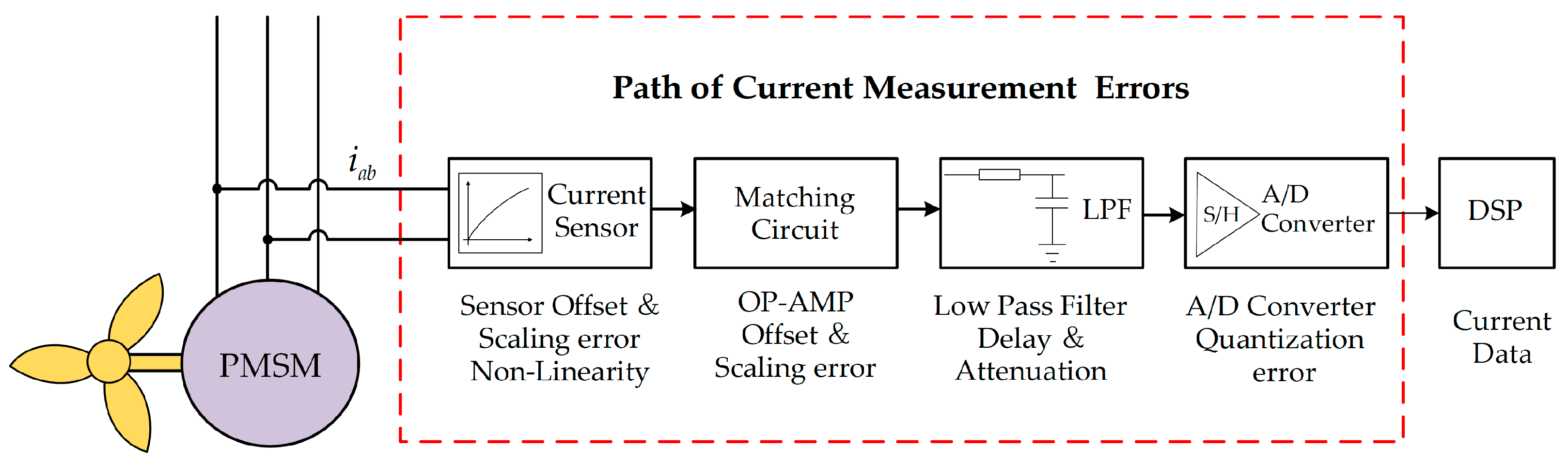
2. Analysis of Current Measurement Errors

2.1. Offset Error

For cost-saving considerations, usually only two current sensors are employed to acquire the phase current values. Thus, three phase measurement currents with offset error are as follows:

$$\begin{array}{c}{i}_{A\_\mathrm{meas1}}=i_A+\Delta i_{A\_\mathrm{offset}}\\ i_{B\_\mathrm{meas1}}=i_B+\Delta i_{B\_\mathrm{offset}}\\ i_{C\_\mathrm{meas1}}=-i_{A\_\mathrm{meas1}}-i_{B\_\mathrm{meas1}}\end{array}$$

(1)

where $i_A$ and $i_B$ are the real phase currents, and ${\mathsf{\Delta }i}_{A\_\mathrm{offset}}$ and ${\mathsf{\Delta }i}_{B\_\mathrm{offset}}$ are the offset errors.

Then, the dq-axes currents, which are calculated from the phase currents through coordinate transformation, can be expressed by Equation (2), and the errors are also preserved.

$$\begin{array}{c}{i}_{d\_\mathrm{meas1}}=i_d+\Delta i_{d\_\mathrm{offset}}\\ i_{q\_\mathrm{meas1}}=i_q+\Delta i_{q\_\mathrm{offset}}\end{array}$$

(2)

where $i_d$ and $i_q$ are real dq-axes currents and, ${\mathsf{\Delta }i}_{d\_\mathrm{offset}}$ and ${\mathsf{\Delta }i}_{q\_\mathrm{offset}}$ are caused by the offset error and expressed as follows:

$$\left[\begin{array}{c}\Delta i_{d\_\mathrm{offset}}\\ \Delta i_{q\_\mathrm{offset}}\end{array}\right]=T_{3\mathrm{s}/2\mathrm{r}}\left[\begin{array}{c}\Delta i_{A\_\mathrm{offset}}\\ \Delta i_{B\_\mathrm{offset}}\\ -\Delta i_{A\_\mathrm{offset}}-\Delta i_{B\_\mathrm{offset}}\end{array}\right]$$

(3)

where ${\mathbf{T}}_{3\mathrm{s}/2\mathrm{r}}$ is the transformation matrix (from the ABC to the dq reference frame). Equation (3) can be expressed as follows:

$$\left\{\begin{array}{c}\Delta i_{d\_\mathrm{offset}}=I_{\mathrm{offset}}\sin ({\omega }_{\mathrm{e}}t+\alpha )\\ \Delta i_{q\_\mathrm{offset}}=I_{\mathrm{offset}}\cos ({\omega }_{\mathrm{e}}t+\alpha )\end{array}\right.$$

(4)

where ${\omega }_{\mathrm{e}}$is the rotational speed in the electrical angle, and the following is obtained:

$$\begin{array}{c}{I}_{\mathrm{offset}}=\frac{2}{\sqrt{3}}\sqrt{\Delta i_{A\_\mathrm{offset}}^2+\Delta i_{A\_\mathrm{offset}}\Delta i_{B\_\mathrm{offset}}+\Delta i_{B\_\mathrm{offset}}^2}\\ \alpha ={\tan }^{-1}(\frac{\sqrt{3}\Delta i_{A\_\mathrm{offset}}}{\Delta i_{A\_\mathrm{offset}}+2\Delta i_{B\_\mathrm{offset}}})\end{array}$$

(5)

When using the vector control method with $i_d=0$, the torque equation can be expressed as:

$$T_{\mathrm{e}}=\frac{3}{2}P{\lambda }_{\mathrm{r}}{i}_{q\_\mathrm{meas1}}=\frac{3}{2}P{\lambda }_{\mathrm{r}}{i}_q+\frac{3}{2}P{\lambda }_{\mathrm{r}}\Delta i_{q\_\mathrm{offset}}=T_{\mathrm{e}\_\mathrm{ref}}+\Delta T_{\mathrm{e}}$$

(6)

where P is the pole pairs of the motor, and ${\lambda }_{\mathrm{r}}$ is the rotor flux. It can be seen that Equation (6) consists of the real value and error value of the torque.

By substituting Equation (4) into Equation (6), ${\mathsf{\Delta }T}_{\mathrm{e}}$ can be expressed as follows:

$$\Delta T_{\mathrm{e}}=\frac{3}{2}P{\lambda }_{\mathrm{r}}{I}_{\mathrm{offset}}\cos ({\omega }_{\mathrm{e}}t+\alpha )$$

(7)

Ignoring the influence of the damping factor, the motion equation of the PMSM is as follows:

$$T_{\mathrm{e}}-T_{\mathrm{L}}=J\frac{d{\omega }_{\mathrm{m}}}{\mathrm{d}t}$$

(8)

where $T_{\mathrm{L}}$ is the load torque, J is the moment of inertia, and ${\omega }_{\mathrm{m}}$ represents the motor speed. Substituting Equation (7) into Equation (8), speed error is determined as follows:

$$\Delta {\omega }_{\mathrm{m}}=\frac{3P{\lambda }_{\mathrm{r}}}{2J{\omega }_{\mathrm{e}}}{I}_{\mathrm{offset}}\sin ({\omega }_{\mathrm{e}}t+\alpha )$$

(9)

It can be seen from Equations (4), (7), and (9) that when there are measurement offset errors in phase currents, there are current ripples with a fundamental frequency in dq-axes currents, which further leads to the presence of the first-order harmonic component in torque and speed.

2.2. Scaling Error

A- and B-phase measurement currents containing scaling errors can be calculated by the following:

$$\begin{array}{l}{i}_{A\_\mathrm{meas2}}=K_{A}I\sin {\theta }_{\mathrm{e}}\\ i_{B\_\mathrm{meas2}}=K_{B}I\sin ({\theta }_{\mathrm{e}}-\frac{2}{3}\pi )\end{array}$$

(10)

where $K_A$ and $K_B$ are scaling gains, and I and ${\theta }_{\mathrm{e}}$ denote current amplitude and stator position, respectively.

Then, dq-axes measurement currents can be calculated from Equation (10) by coordinate transformation. The currents are given by the following:

$$\begin{array}{c}{i}_{d\_\mathrm{meas2}}=\frac{K_A-K_B}{\sqrt{3}}I\sin (2{\theta }_{\mathrm{e}}-\frac{1}{6}\pi )+\frac{K_A-K_B}{2\sqrt{3}}I\\ i_{q\_\mathrm{meas2}}=\frac{K_A-K_B}{\sqrt{3}}I\sin (2{\theta }_{\mathrm{e}}+\frac{1}{3}\pi )+\frac{K_A+K_B}{2}I\end{array}$$

(11)

If there are no differential scaling errors, that is, if $K_A=K_B$, $i_d$ and $i_q$ are 0, and $\frac{K_A+K_B}{2}I$, respectively, then it is easy to see that a second-order harmonic pulsating component is introduced into the dq-axes current due to the scaling error. Based on the previous analysis of Equations (6)–(9), a second-order harmonic component is also introduced into the motor’s torque and speed.

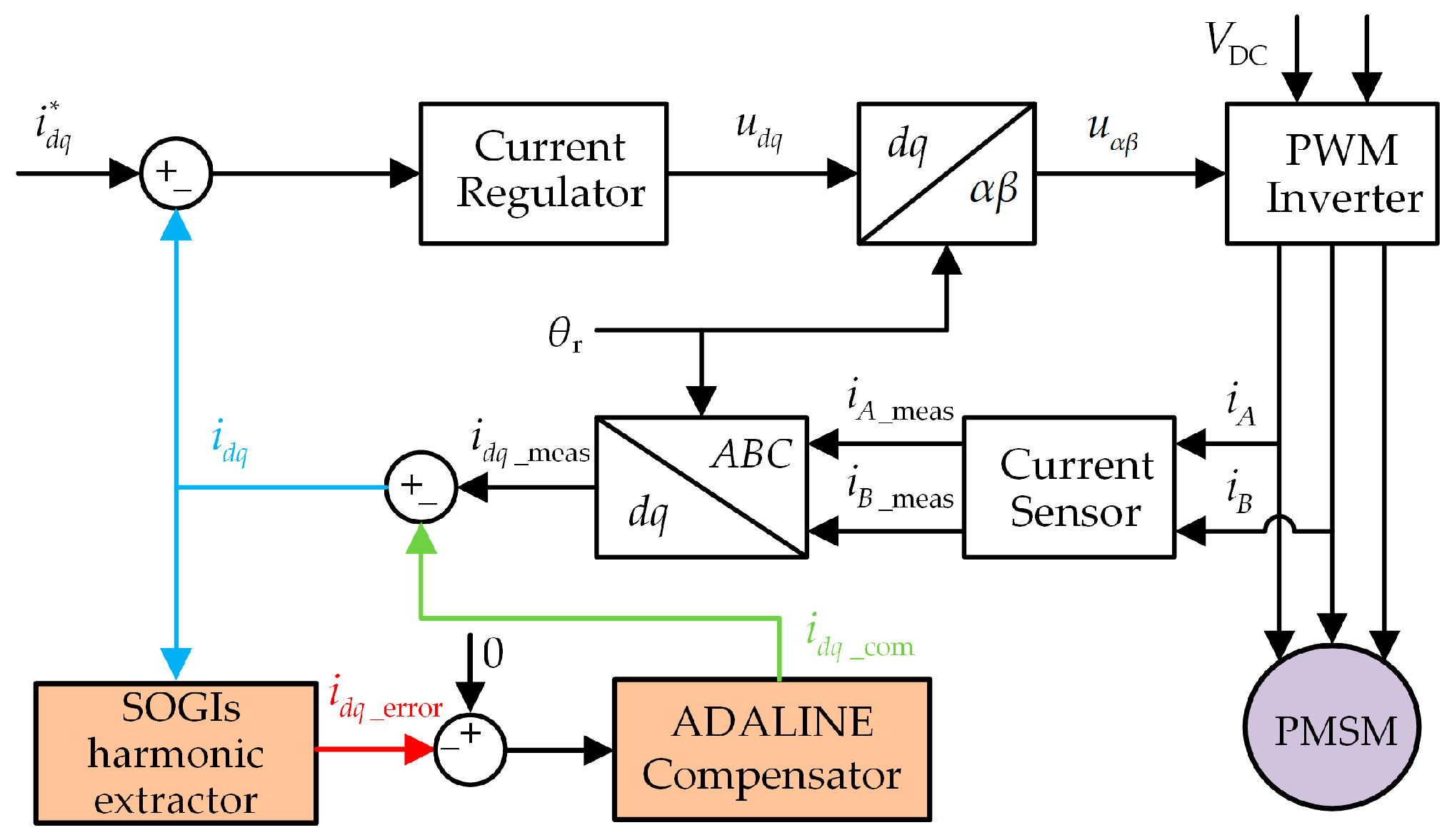
3. Proposed Strategy for Compensating Current Measurement Errors

Figure 2 shows that the current measurement errors are located in the current loop feedback channel and affect the dq-axes current. According to the analysis of Equations (1)–(11), errors can also cause fluctuations in motor torque and speed. Therefore, it is necessary to propose a strategy with an excellent performance to eliminate the fluctuations. However, the current controller cannot suppress the disturbance in the feedback channel, so Ref. [15] designed a proportional resonance controller in the speed loop to minimize the impact of errors in current measurements. However, the harmonics of the d-axis current still affects the motor. Hence, this study presents a method to compensate for the errors in dq-axes feedback channels simultaneously.

The 1st- and 2nd-order current harmonics analyzed in Section 2 should be compensated to 0 for the improvement in PMSM control performance. Hence, it is better to have knowledge about the existing current harmonics information to easily determine the compensation values. In this paper, accurate extraction of the 1st- and 2nd-order dq-axes current harmonics is achieved using the cascade decoupling SOGIs. Next, the compensation values for these harmonics are generated by a feedback compensator based on the ADALINE algorithm. A diagram with the proposed compensation strategy is depicted in Figure 2.

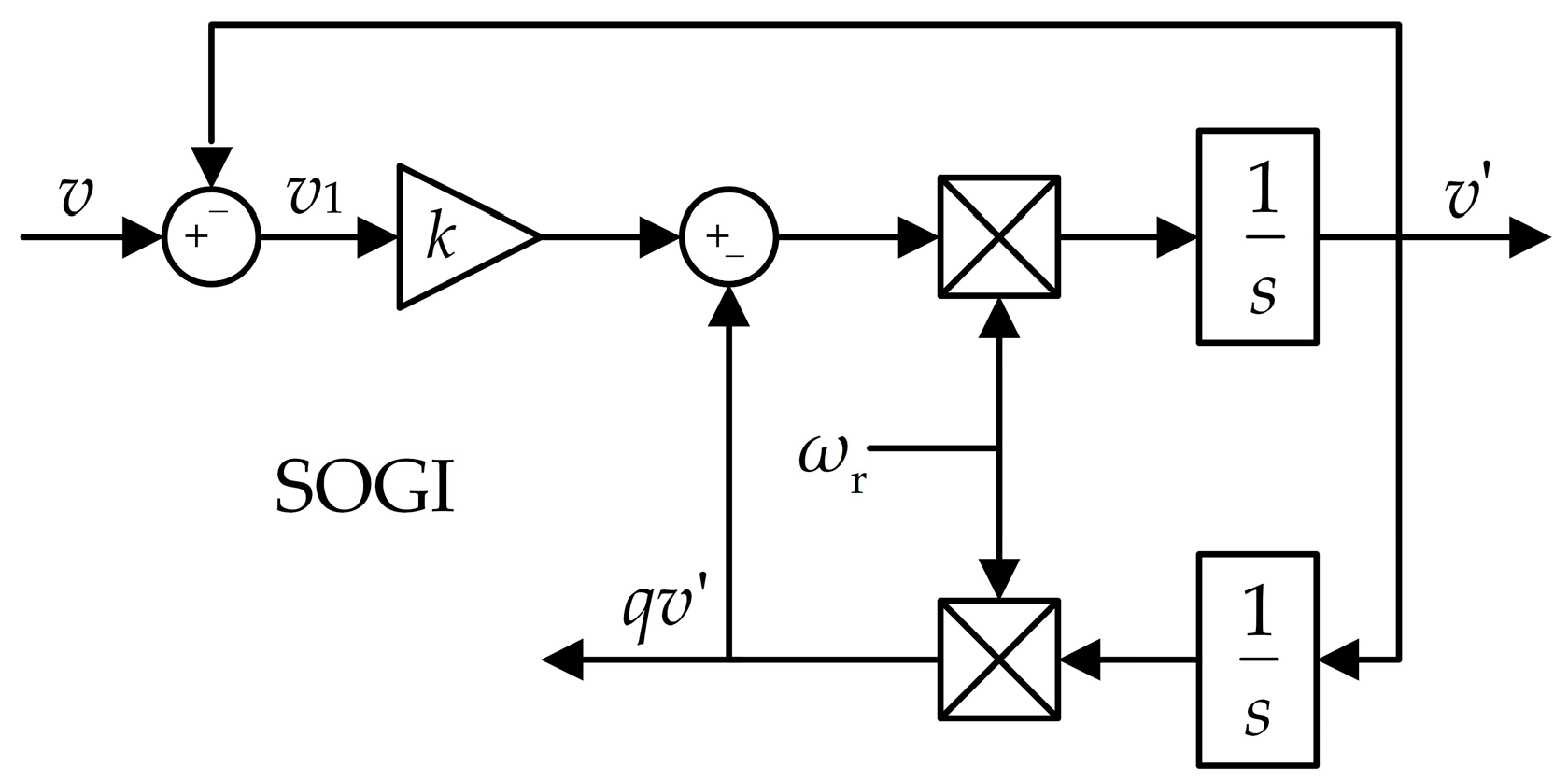
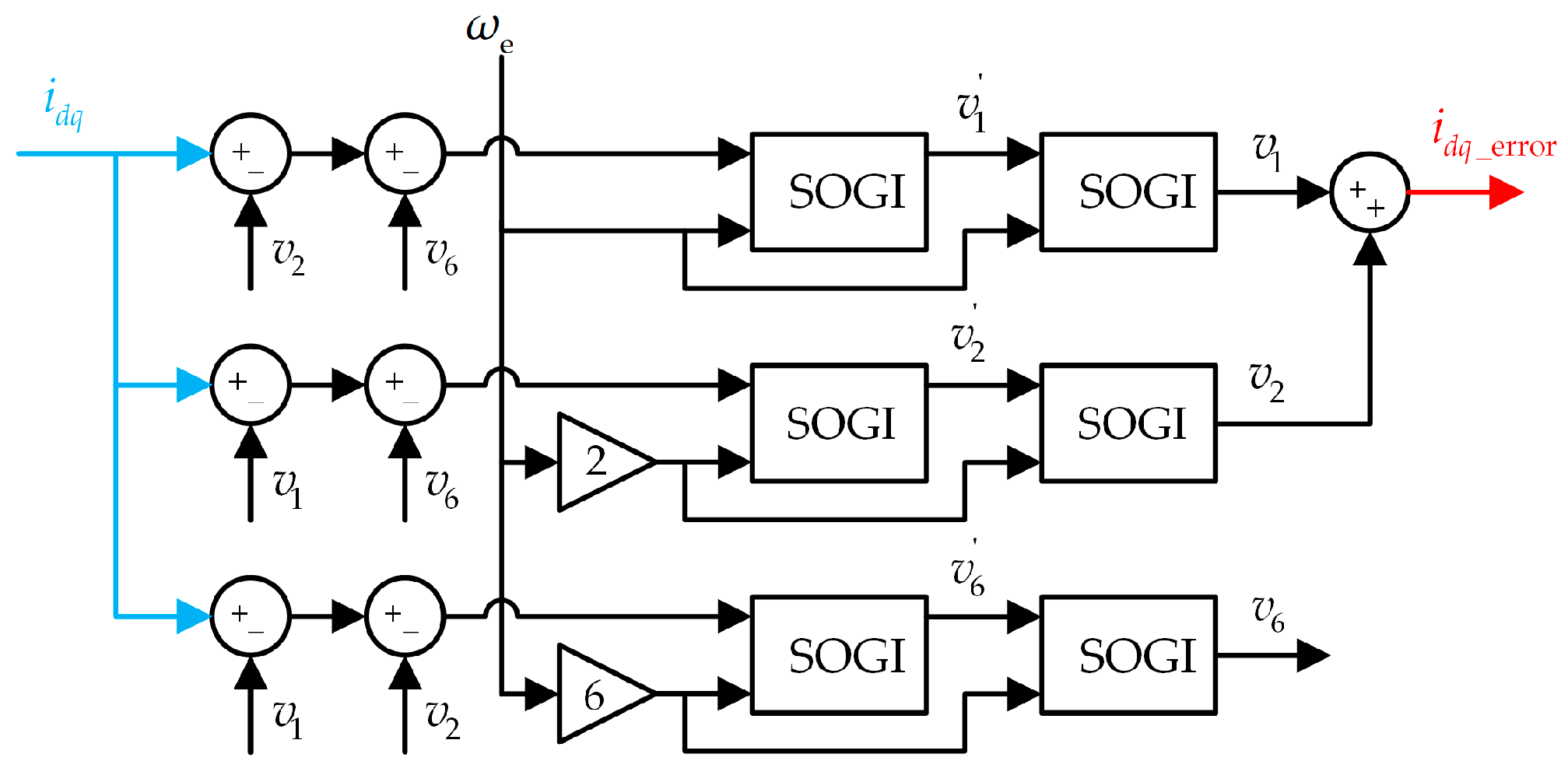
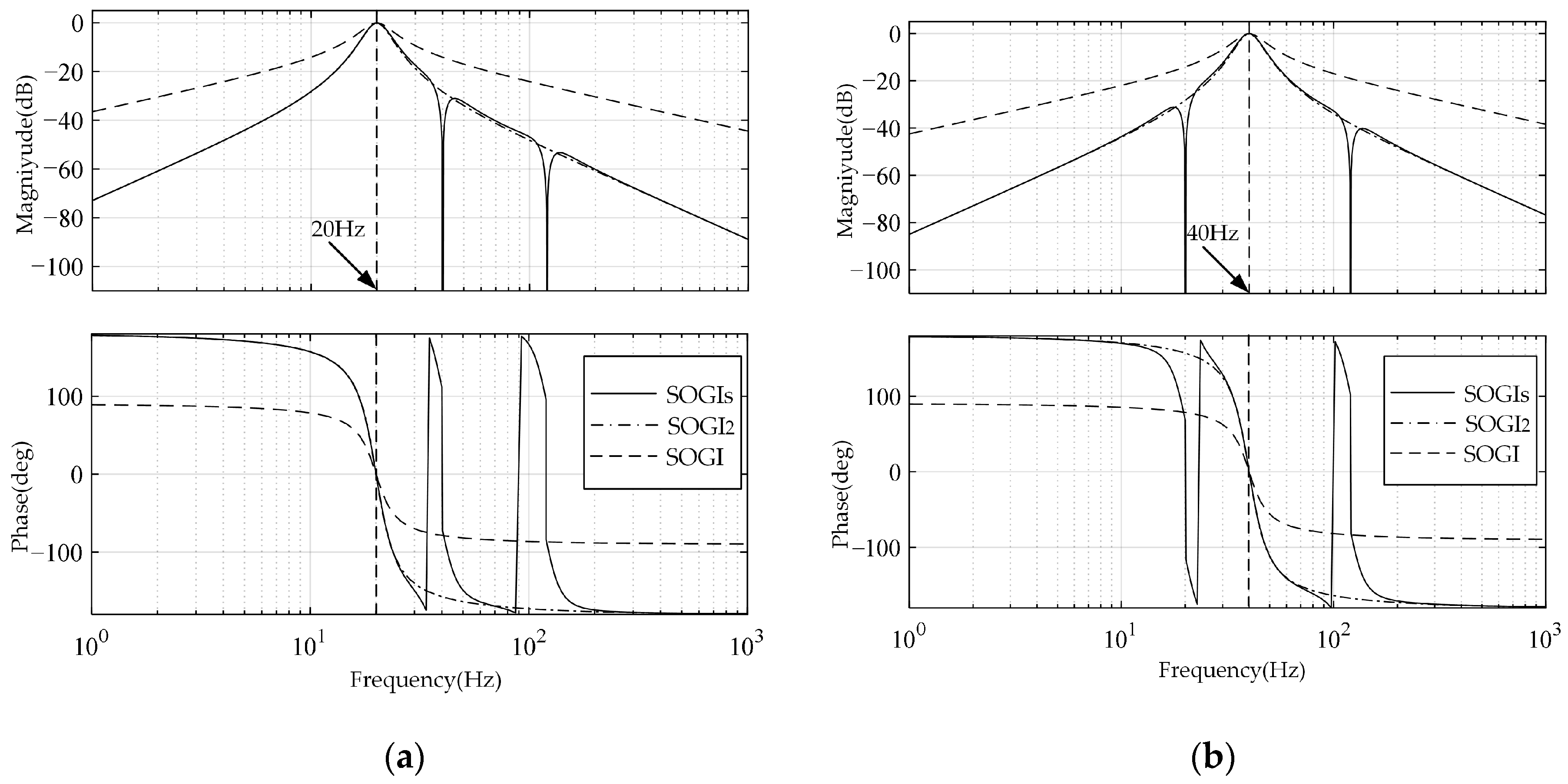
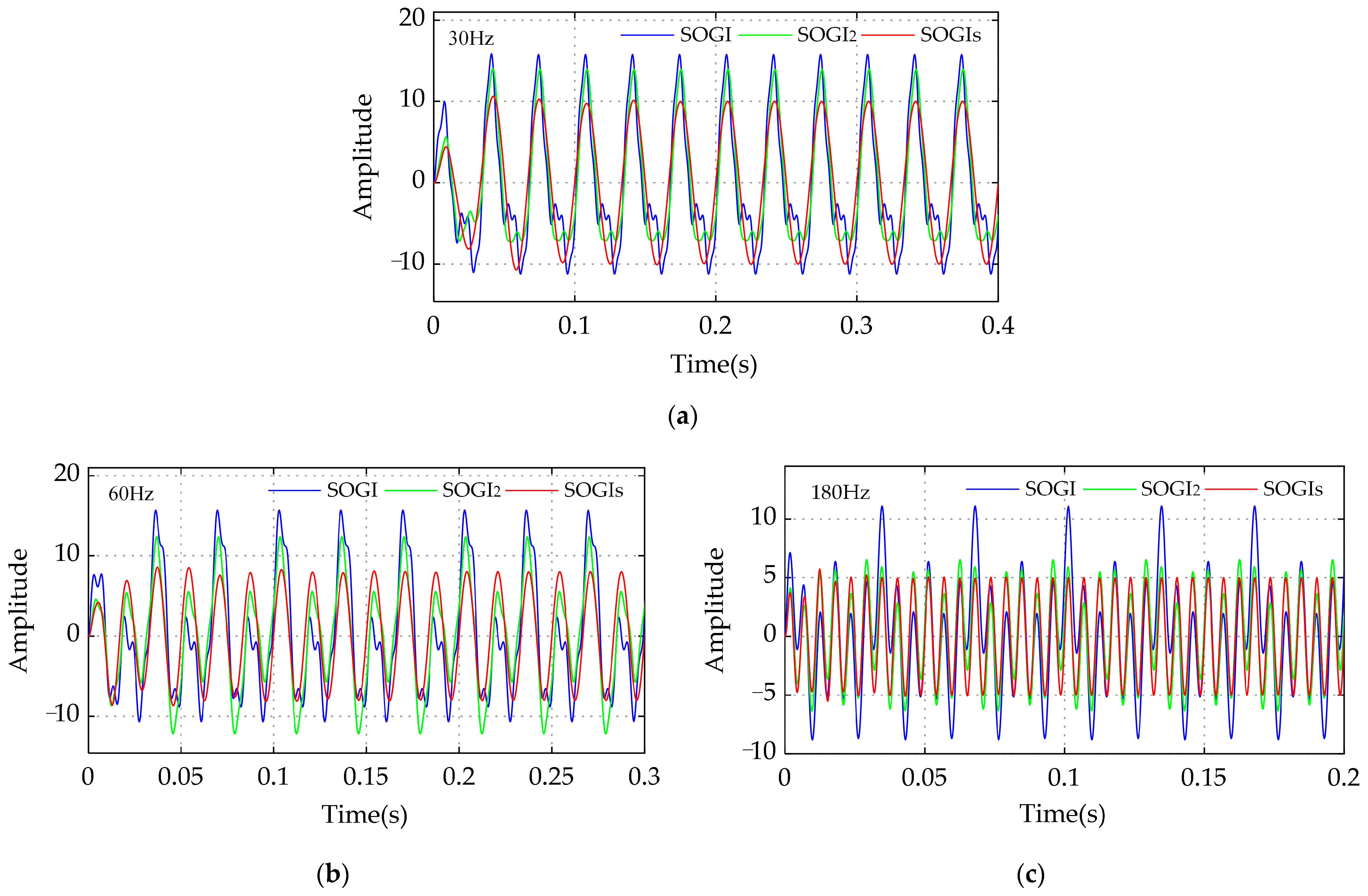
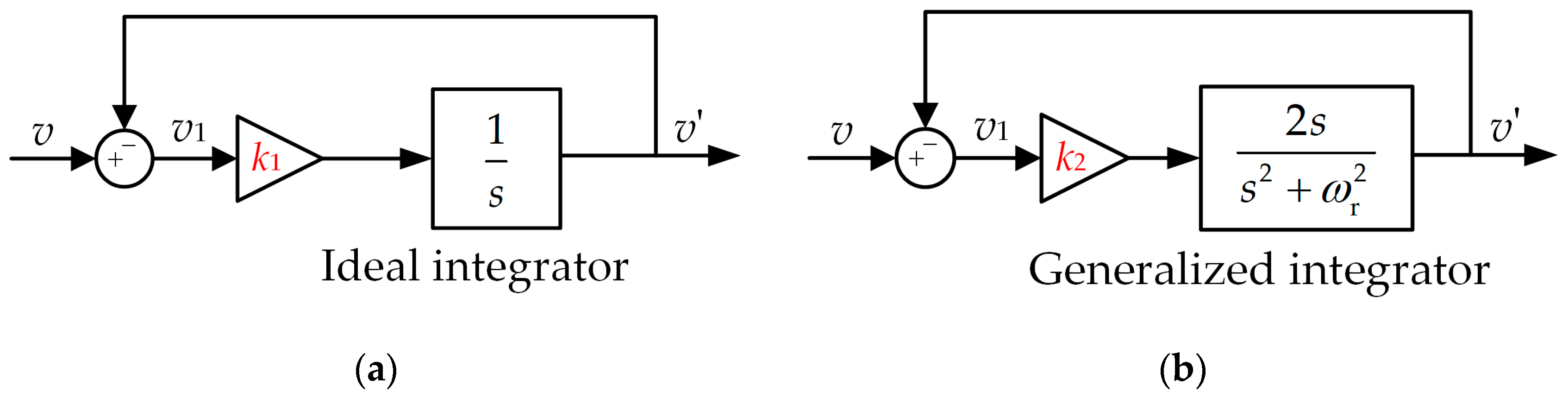
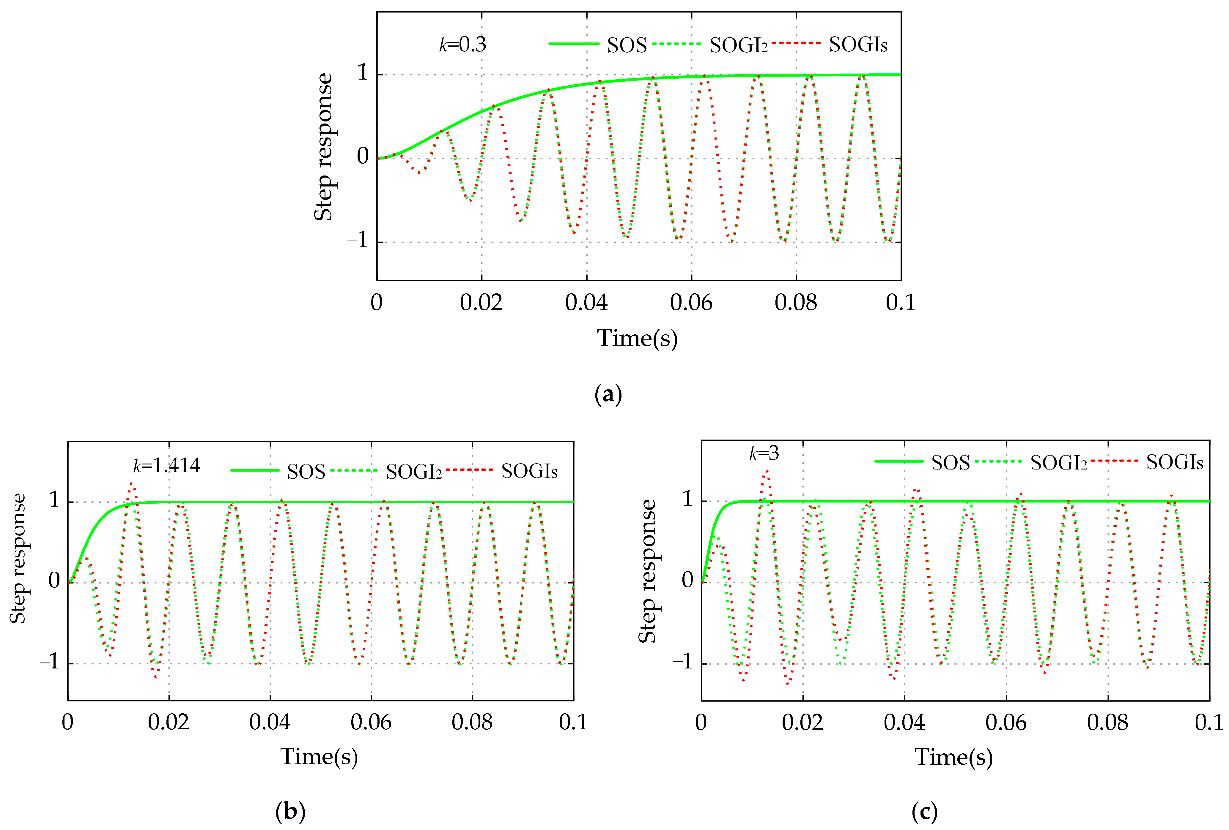
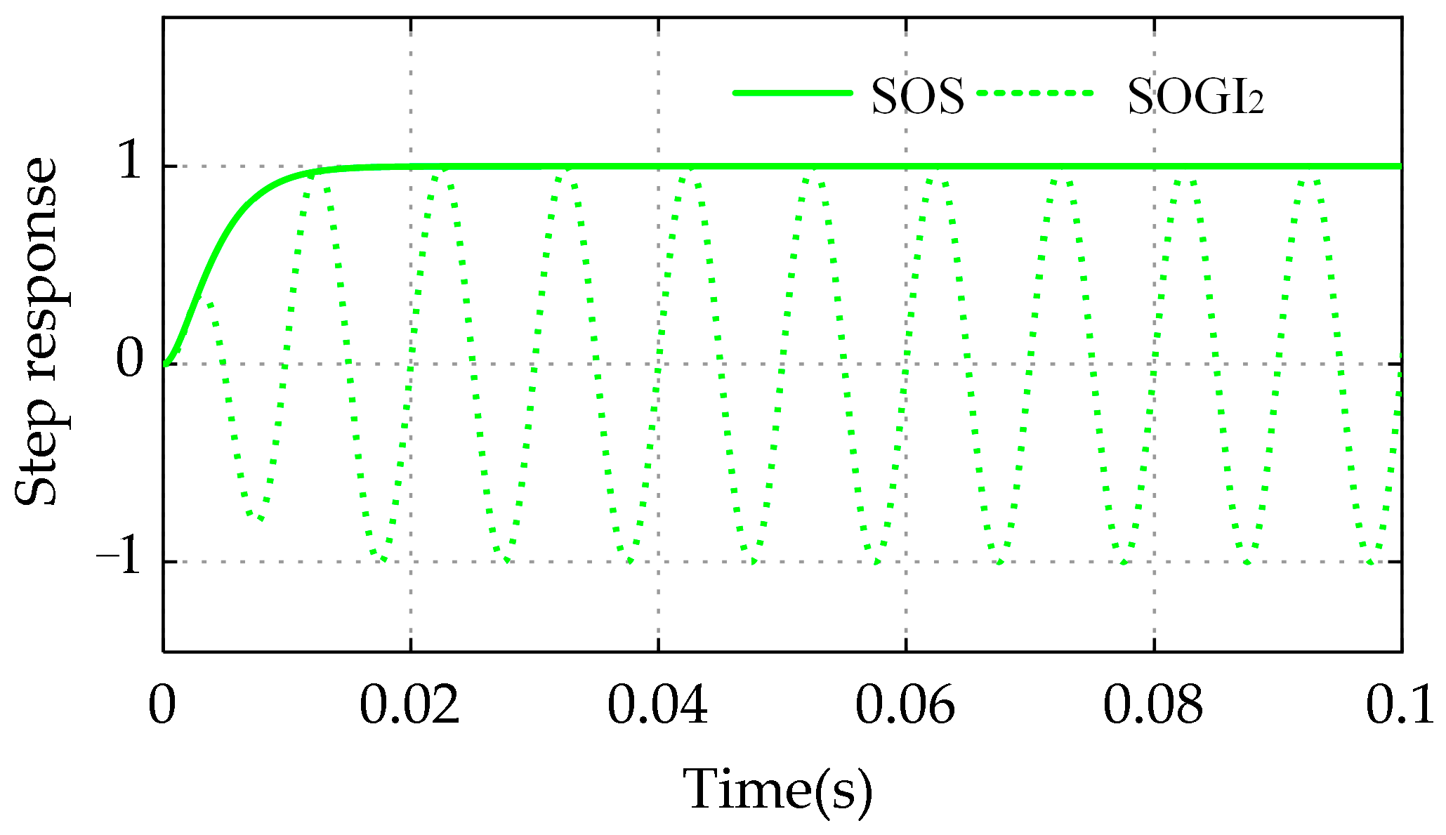
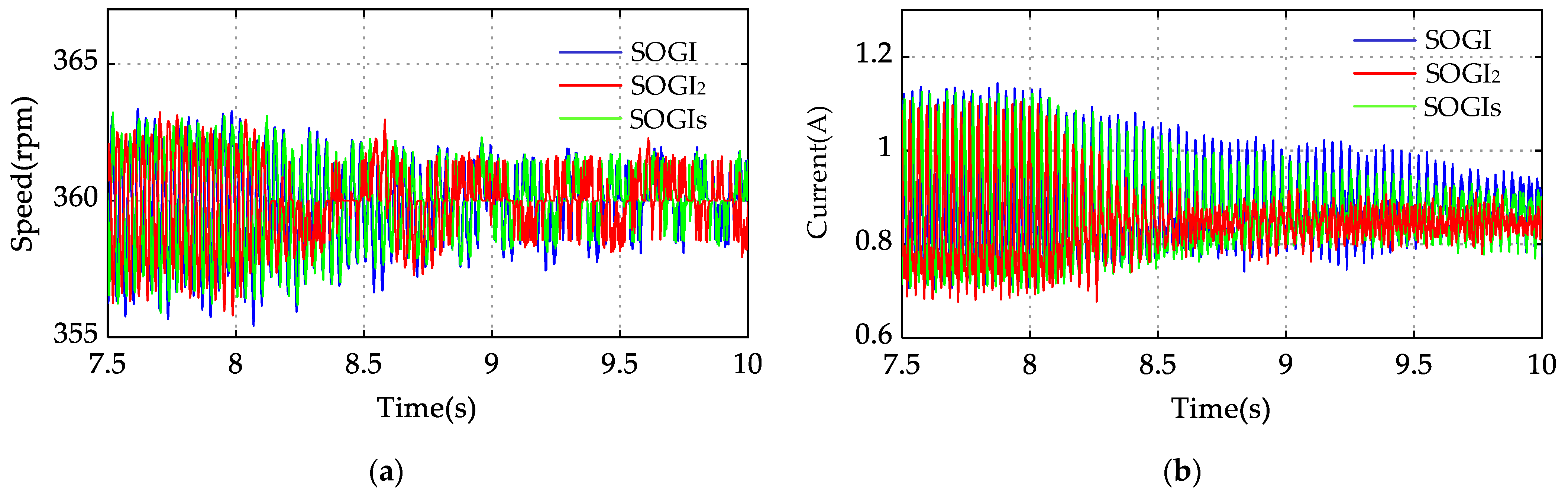
3.1. Cascade Decoupling SOGIs

The SOGI in Figure 3 can be used as a filter to select or eliminate the components at a specific frequency. In Figure 3, ${\omega }_{\mathrm{r}}$ represents the resonance frequency of the SOGI. The output $v^{\prime }$ is the component at the frequency of ${\omega }_{\mathrm{r}}$ extracted from the input signal v. The output $q{v}^{\prime }$ has the same frequency and amplitude as $v^{\prime }$; however, their phases are orthogonal. SOGI’s transfer function can be expressed as follows:

$$D(s)=\frac{v^{\prime }}{v}(s)=\frac{k{\omega }_{\mathrm{r}}s}{s^2+k{\omega }_{\mathrm{r}}s+{\omega }_{\mathrm{r}}^2}$$

(12)

SOGI is a bandpass filter. The bandwidth is determined by the gain k and is independent of the resonance frequency ${\omega }_{\mathrm{r}}$. The smaller the value of k set, the narrower the bandwidth becomes.

Compared with the Fourier-based harmonic detection method, the SOGI requires less DSP computation power and is able to provide more precise results under transient conditions [38]. However, the harmonics in the motor are too closely spaced when operating at low speed, resulting in significant distortion in the harmonic components extracted by the SOGI. In addition, the currents may also contain other order harmonics, such as 6th-order harmonics ripples, due to inverter nonlinearity. The accuracy of the extraction may also be affected. The performance may be improved by taking a narrower bandwidth. However, too small a gain k results in a slow response to signal extraction [29]. To reduce the effects of various harmonics and ensure the dynamic performance simultaneously, a cascade decoupling SOGI structure is proposed in Figure 4.

A cross-feedback decoupling network is used in this structure, which effectively isolates the influence of various harmonics. The resonance frequency for each branch is given by ${n\omega }_{\mathrm{r}}$, where ${\omega }_{\mathrm{r}}$ is equal to ${\omega }_{\mathrm{e}}$ and n is the harmonic order. In each branch, a SOGI₂ (two SOGIs in series) is used. The first SOGI is used as a bandpass prefilter, which can overcome the limitations of the single SOGI without affecting the system response [28]. The second one is utilized for extracting the harmonic current at the fundamental frequency.

For the series connection of two SOGI structures (SOGI₂) with the same fundamental frequencies, the transfer function is as follows:

$$G_n(s)=D_n^2(s)={\left(\frac{k(n{\omega }_{\mathrm{r}})s}{s^2+k(n{\omega }_{\mathrm{r}})s+{(n{\omega }_{\mathrm{r}})}^2}\right)}^2$$

(13)

Then, the outputs $v_n$ of each branch can be expressed as follows:

$$\begin{array}{c}{v}_1=G_1(s)(v-v_2-v_6)\\ v_2=G_2(s)(v-v_1-v_6)\\ v_6=G_6(s)(v-v_1-v_2)\end{array}$$

(14)

According to Equations (13) and (14), the transfer functions of the structure in Figure 4 are given by Equations (15) and (16):

$$\frac{v_1}{v}(s)=G_1\frac{1-G_2-G_6+G_2{G}_6}{1-G_1{G}_2-G_2{G}_6-G_1{G}_6+G_1{G}_2{G}_6}$$

(15)

$$\frac{v_2}{v}(s)=G_2\frac{1-G_1-G_6+G_1{G}_6}{1-G_1{G}_2-G_2{G}_6-G_1{G}_6+G_1{G}_2{G}_6}$$

(16)

Equations (12) and (13) are the transfer functions of the SOGI and the SOGI₂, respectively, and Equations (15) and (16) are the transfer functions of the cascade decoupling SOGIs. Equation (12) shows that the SOGI transfer function becomes 1 at the resonant frequency ${\omega }_{\mathrm{r}}$, indicating that the SOGI has an amplitude–frequency response of 1 and a phase–frequency response of 0. In the same way, the SOGI₂ and cascade decoupling SOGIs also possess these features.

Figure 5 shows the Bode diagrams of the three SOGI structures.

It can be seen from Figure 5 that the cascade decoupling SOGIs not only exhibit amplitude–frequency characteristics of 1 and phase–frequency characteristics of 0 at the resonant frequency ${\omega }_{\mathrm{r}}$, but also effectively attenuate DC offset and other harmonic signals in different frequency bands. It exhibits notch characteristics at the other two harmonic frequencies and can accurately extract the required harmonic signals. These signals can then be used in the ADALINE compensator to effectively compensate for current harmonics.

In addition, this paper also provides the simulation and comparison of the 1st-, 2nd-, and 6th-order harmonic extraction waveforms of a single SOGI, the SOGI₂, and the cascade decoupling SOGIs, as shown in Figure 6. The simulation input of both structures is a sum of sinusoidal signals with fundamental frequencies of 30 Hz, 60 Hz, and 180 Hz, and amplitudes of 10, 8, and 5, respectively, with k = 1.414 and the fundamental frequency references of the SOGI(s) being 30 Hz, 60 Hz, and 180 Hz, respectively.

Figure 6 shows the simulation results and

Table 2. Analysis results of Figure 6 using Fourier analysis method.

Harmonic Content	${\mathit{\omega }}_{\mathbf{r}}=30 \mathbf{H}\mathbf{z}$			${\mathit{\omega }}_{\mathbf{r}}=60 \mathbf{H}\mathbf{z}$			${\mathit{\omega }}_{\mathbf{r}}=180 \mathbf{H}\mathbf{z}$
	SOGI	SOGI2	SOGIs	SOGI	SOGI2	SOGIs	SOGI	SOGI2	SOGIs
30 Hz	10	10	10	6.86	5.74	0	2.89	0.75	0
60 Hz	5.49	3.76	0	8	8	8	4.75	1.77	0
180 Hz	1.18	0.28	0	2.34	1.06	0	5	5	5

records the analysis results of Figure 6 using the Fourier analysis method. The results indicate that the signal extracted by cascade decoupling SOGIs is almost pure, with no other harmonics present. However, the output of the single SOGI and the SOGI₂ is clearly distorted. Hence, the extraction accuracy of the cascade decoupling SOGIs is better.

To better clarify the impact of parameters on the extractor. Ref. [39] shows that the amplitude response of the SOGI is equivalent to the first-order system $\frac{k_1}{s+k_1}$.

The transfer function of the SOGI block depicted in Figure 3 can be replaced with the generalized integrator (GI) in [39]. The resulting equivalent structure is illustrated in Figure 7b, with k₂ being set to kω_r/2. The GI in Figure 7b can perform amplitude integration when a sinusoidal signal is input [39]. Therefore, the amplitude response shown in Figure 7b will be similar to the amplitude response of an ideal integrator when a DC signal is input [39].

Similarly, the SOGI₂ (two SOGIs in series) of the manuscript can be equivalent to two first-order systems in series; that is, the equivalent transfer function is as follows:

$$G(s)=\frac{k_1}{s+k_1}\frac{k_1}{s+k_1}=\frac{k_1{}^2}{s^2+2k_{1}s+k_1{}^2}$$

(17)

The above equation shows that if the gain coefficients of the front and rear SOGI are equal, the amplitude response of the SOGI₂ to the AC signal can be equivalent to the amplitude response of the critically damped second-order system to the DC signal. To illustrate this point, a sinusoidal signal v(t) = sin (200πt) is fed to the input of the SOGI₂; its output response with k₁ = k₂ = 1.414 × 200 × π/2 and ω_r = 200π rad/s (or k = 1.414) is shown in Figure 8, together with the step response of the second-order system (SOS) (G(s) in Equation (17).

Next, the amplitude response of the cascaded decoupled SOGIs is analyzed. From Equation (17), it can be seen that when k₁ is larger (the larger k is), the response speed of the system is faster. However, excessively large parameters will deteriorate the frequency selection performance of the SOGI and cause other interference harmonics to be introduced into the system (such as the 6th harmonic). For SOGIs, parameters that are too large will also cause fluctuations in the extracted signal (see the figure below). Therefore, the speed and accuracy of the harmonic extractor need to be considered comprehensively. To clarify this point, the amplitude response simulation results of three structures with different gain coefficients are shown in Figure 9. In addition, the SOGI parameters selected in Refs. [29,32,39] range from 0.3 to 3.11. Combined with the above analysis, we conducted a set of comparative experiments under different parameters.

Finally, the structure and parameters of the SOGI extractor in the motor system are determined.

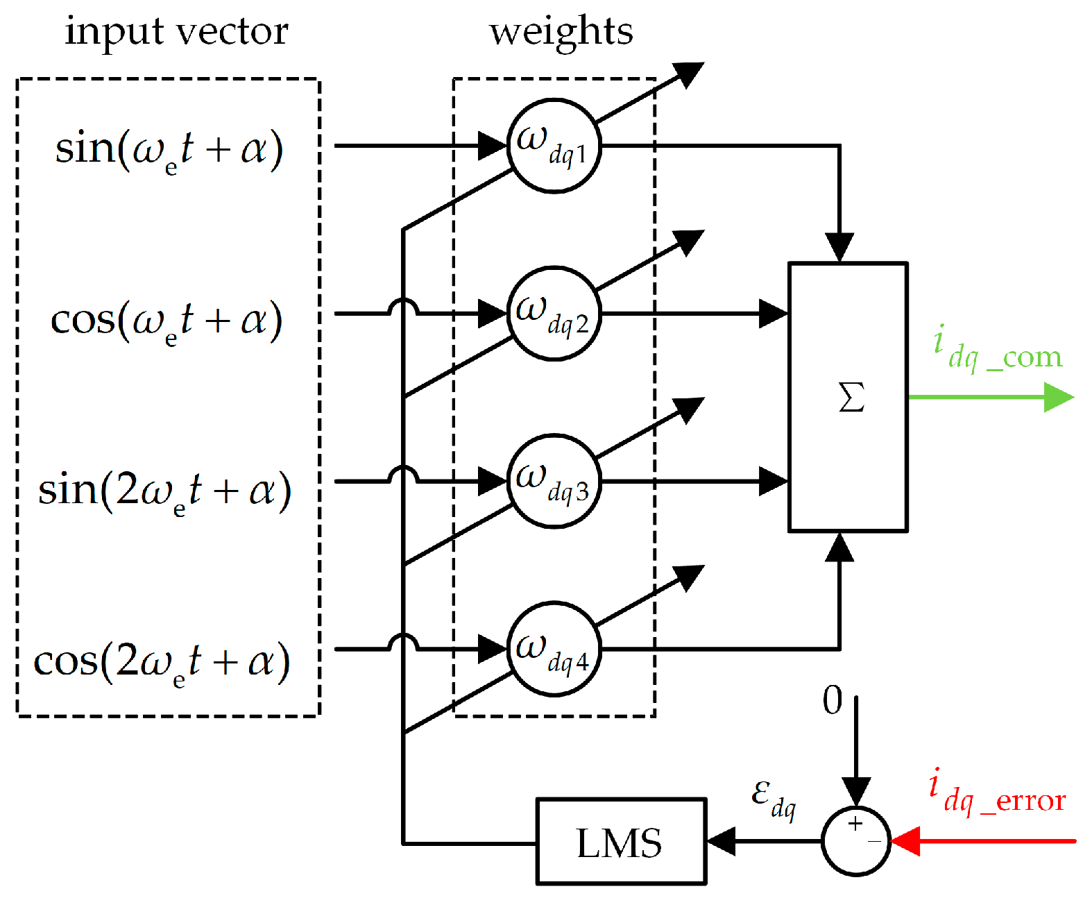
3.2. Compensation Based on ADALINEs

Figure 10 illustrates the structure of the compensators for the dq-axes current ADALINE network. It consists of multiple inputs, a single output, and a single layer linear neural network. The neural network weights can be trained online by updating the algorithm according to the error between the current harmonics and the expected zero value. Therefore, it is widely used as a filter in the fields of motor control [40,41]. In actual industrial control situations, processor performance is often severely limited and can only execute simpler algorithms. Therefore, adaptive linear neural networks with low computational requirements have greater applicability. This paper utilizes the resonance characteristics of the ADALINE algorithm to design a harmonic compensator that can simultaneously compensate for the 1st- and 2nd-order harmonics of the dq-axes current. To compensate for the current harmonics caused by measurement errors, two current compensators are used on the dq-axes, respectively. The d-axis current decomposition is analyzed comprehensively, and the findings can be extrapolated to the q-axis. According to the previous analysis, $i_{d\_\mathrm{meas}}$ can be expressed by Equation (18):

$$\begin{array}{r}{i}_{d\_\mathrm{meas}}=a_0+a_1\sin ({\omega }_{\mathrm{e}}t+\alpha )+b_1\cos ({\omega }_{\mathrm{e}}t+\alpha )\\ +a_2\sin (2{\omega }_{\mathrm{e}}t+\alpha )+b_2\cos (2{\omega }_{\mathrm{e}}t+\alpha )\end{array}$$

(18)

where $a_0$ is a DC component which is 0 for $i_d$ and a constant for $i_q$. $a_1$, $b_1$, $a_2$, and $b_2$ represent the magnitudes of the other terms in the Fourier expansion formula. ${\omega }_{\mathrm{e}}t$ represents the electrical angle of the PMSM, which can be obtained from an encoder during experimental testing.

To eliminate the harmonics, the compensating current $i_{d\_\mathrm{com}}$ is as follows:

$$\begin{array}{l}{i}_{d\_\mathrm{com}}=W_d{X}_d^{\mathrm{T}}\\ ={\omega }_{d1}\sin ({\omega }_{\mathrm{e}}t+\alpha )+{\omega }_{d2}\cos ({\omega }_{\mathrm{e}}t+\alpha )\\ +{\omega }_{d3}\sin (2{\omega }_{\mathrm{e}}t+\alpha )+{\omega }_{d4}\cos (2{\omega }_{\mathrm{e}}t+\alpha )\end{array}$$

(19)

where ${\mathbf{X}}_d=[\sin ({\omega }_{\mathrm{e}}t+\alpha )\cos ({\omega }_{\mathrm{e}}t+\alpha )\sin (2{\omega }_{\mathrm{e}}t+\alpha )\cos (2{\omega }_{\mathrm{e}}t+\alpha \left)\right]$ and ${\mathbf{W}}_d=[{\omega }_{d1}{\omega }_{d2}{\omega }_{d3}{\omega }_{d4}]$ and they are the input vector and the weight vector of the d-axis current compensator, respectively.

The weights are computed utilizing the least mean square (LMS) algorithm, a widely employed method in adaptive control owing to its straightforward design and robustness [40,42]. The updated rule is given by Equation (20).

$$W_d(k+1)=W_d(k)+\eta {\epsilon }_d{X}_d$$

(20)

where $\eta$ represents the learning rate of the compensator, which determines the convergence speed and stability of ADALINEs. The larger the learning rate, the wider the bandwidth and the greater the impact on system stability. With a smaller learning rate, the system robustness to disturbance decreases and the convergence speed slows down.

The learning rate in this paper is set to 0.001. ${\epsilon }_d$ is the feedback error that is given by the following:

$${\epsilon }_d=0-i_{d\_error}$$

(21)

where $i_{d\_\mathrm{error}}$ is the summation of the 1st- and 2nd-order current harmonics extracted by the SOGIs. The compensating current for the q-axis is determined using a similar approach.

The transfer function of ADALINEs is as follows [41]:

$$G_A(z)=\eta \left(\frac{z\cos ({\omega }_{e}T)-1}{z^2-2z\cos ({\omega }_{e}T)+1}+\frac{z\cos (2{\omega }_{e}T)-1}{z^2-2z\cos (2{\omega }_{e}T)+1}\right)$$

(22)

The amplitude–frequency characteristics of the ADALINE compensator with different learning rates are shown in Figure 11. The ADALINE network has infinite gain at the relevant frequency, which means that it can perfectly track/suppress periodic signals (according to the internal model principle). Therefore, the compensator based on ADALINE can fully compensate for the current harmonics of the dq-axes caused by current measurement errors. Therefore, the overall control block diagram of the proposed compensation structure is shown in Figure 12. As depicted in the figure, this structure only needs to operate within the current loop and is suitable for control systems without a speed outer loop, such as the motor torque control mode of electric vehicles.

In summary, the proposed method utilizes cascade decoupling SOGIs to accurately extract the 1st-order and 2nd-order harmonics of the dq-axes current. Subtract the pulsating component from 0, and use the resulting difference ${\epsilon }_d$ as the input reference signal for the ADALINE compensator. As shown in Figure 10, the ADALINE compensator uses the LMS algorithm to update the weight of the input vector ${\mathbf{X}}_d=[\sin ({\omega }_{\mathrm{e}}t+\alpha )\cos ({\omega }_{\mathrm{e}}t+\alpha )\sin (2{\omega }_{\mathrm{e}}t+\alpha )\cos (2{\omega }_{\mathrm{e}}t+\alpha \left)\right],$thereby continuously changing the output vector until the input reference deviation ${\epsilon }_d$reaches 0. After multiple iterations, the dq-axes current compensation value $i_{\mathit{dq}\_\mathrm{com}}$ outputted by the ADALINE compensator tends to stabilize; the dq-axes current ripples have also been effectively suppressed.

4. Experimental Results

A motorized towing platform is commonly used to assess the effectiveness of new motion system control strategies. Ref. [43] verified the effectiveness of the proposed power compensation strategy for a shipboard propulsion system using a small experimental platform with two doubly fed induction machines. Ref. [44] verified the stability of a low-power electronics-integrated electric shipboard propulsion system by conducting tests on a small induction motor platform in the laboratory.

To assess the efficacy of the proposed method, experiments were carried out on a PMSM platform. As shown in Figure 13, two PMSMs are used as the driving motor and the load motor, respectively. And their parameters are specified in

Table 3. Parameters of the PMSM in Figure 13.

Parameters	Value
Pole pairs	5
Stator resistance (Ω)	1.616
d-axis stator inductance (mH)	11.47
q-axis stator inductance (mH)	11.47
Flux linkage (Wb)	0.231
Rated current (A)	5
Supply voltage (V)	300
Moment of inertia (kg·m2)	0.00235
Rated power (W)	1000
Rated torque (N·m)	9.55
Rated speed (rpm)	1000

. The motors are controlled by two TMDSCNCD28379D control cards (Texas Instruments Semiconductor Technologies Co., Ltd., Dallas, TX, USA), and two IDDK v2.2 boards are used as voltage source inverters. The motor’s position and speed are determined by a 2500-wire incremental encoder. Both the switching frequency and the sampling frequency are configured at 10 kHz. The control board communicates with the host computer in real time through the serial port. The software algorithms are automatically generated using the rapid control prototyping development method of model-based design (MBD). It is developed using MATLAB (2022b)/Simulink and is capable of automatically generating C code. It achieves dual closed-loop real-time control of motor current and speed. Additionally, it features a computer monitoring interface that allows for the online adjustment of control parameters and the storage of collected data. The current measurement errors are described by Equation (23).

$$\begin{array}{l}\mathsf{\Delta }{i}_{A\_\mathrm{offset}}=0.1\mathrm{A} K_A=1.1\\ \mathsf{\Delta }{i}_{B\_\mathrm{offset}}=-0.15\mathrm{A} K_B=0.9\end{array}$$

(23)

4.1. Parameter Determination

The primary parameters to be identified for the method outlined in this paper are the gain k of the SOGI and the learning rate η of the ADALINE compensator. Figure 14a depicts the speed waveform with the k-value when the compensation method is applied at 8 s. The results indicate that the speed waveform converges slowly when the k-value is small. When the k-value is high, the speed fluctuates when using the compensation method. When k = 1.414, the speed can smoothly and rapidly converge to the stable range. After careful consideration, the k-value of the cascade decoupling SOGIs parameter has been determined to be 1.414.

A comparative experiment with different learning rates has been conducted. The experimental results in Figure 14b indicate that the system’s convergence rate is slow when the learning rate is small. Increasing the learning rate can speed up the system’s convergence. However, the system becomes unstable when the learning rate is excessively high. The results also demonstrate that the system is capable of achieving satisfactory stability and convergence when the learning rate of the ADALINE network varies within a specific range. The proposed method is insensitive to the learning rate of the ADALINE network, which is also one of its advantages. Therefore, a learning rate of 0.001 has been set for the subsequent experiments.

4.2. Steady-State Performance

Figure 15 depicts the experimental results obtained at 360 rpm, with the current measurement errors introduced at 16 s. Figure 15a shows the speed, $i_{\mathit{dq}}$ and $i_{\mathit{dq}\_\mathrm{error}}$, extracted by the cascade decoupling SOGIs without compensation. When measurement errors are injected and no compensating strategy is applied, both the speed ripple and current ripple increase. The harmonic contents of the first- and second-order harmonics in the q-axis current are 8.24% and 2.72%, respectively. Figure 15b shows the results of the speed, the dq-axes currents, and the compensating currents $i_{\mathit{dq}\_\mathrm{com}}$ generated by the ADALINE network when the compensating strategy is used. After a brief fluctuation, the speed and currents quickly converge and remain stable as the compensation currents increase to match the harmonic currents. The harmonic contents decrease to 3.28% and 1.63%, which demonstrates the effectiveness of the proposed compensating strategy at a steady state.

To illustrate the effect of the proposed approach in mitigating phase current distortion and speed/torque ripple, comparative tests are conducted before and after compensation. The findings are depicted in Figure 16, and the corresponding FFT analysis is presented in

Table 4. FFT analysis results of Figure 16.

Harmonic Content		A-Phase (A)	B-Phase (A)	Speed (rpm)	Torque (N·m)
Before compensation	dc	0.0799	0.0836	449.91	2.7828
	1st	1.7475	1.5987	1.2106	0.3035
	2nd	0.0089	0.0047	0.9895	0.3171
	THD	4.81%	3.68%	0.44%	16.12%
After compensation	dc	0.0064	0.0076	449.92	2.7750
	1st	1.7250	1.7580	0.1676	0.1341
	2nd	0.0038	0.0018	0.1338	0.0634
	THD	1.89%	1.72%	0.18%	5.63%

. In the experiment, the proposed method is introduced at 8 s. According to Figure 16, after compensation, the current imbalance between phase A and phase B has been significantly improved, leading to a substantial reduction in the motor’s speed and torque ripples. The results in Table 4 show that the imbalance degree of the phase current decreases from 9.8% to 1.7% after compensation.

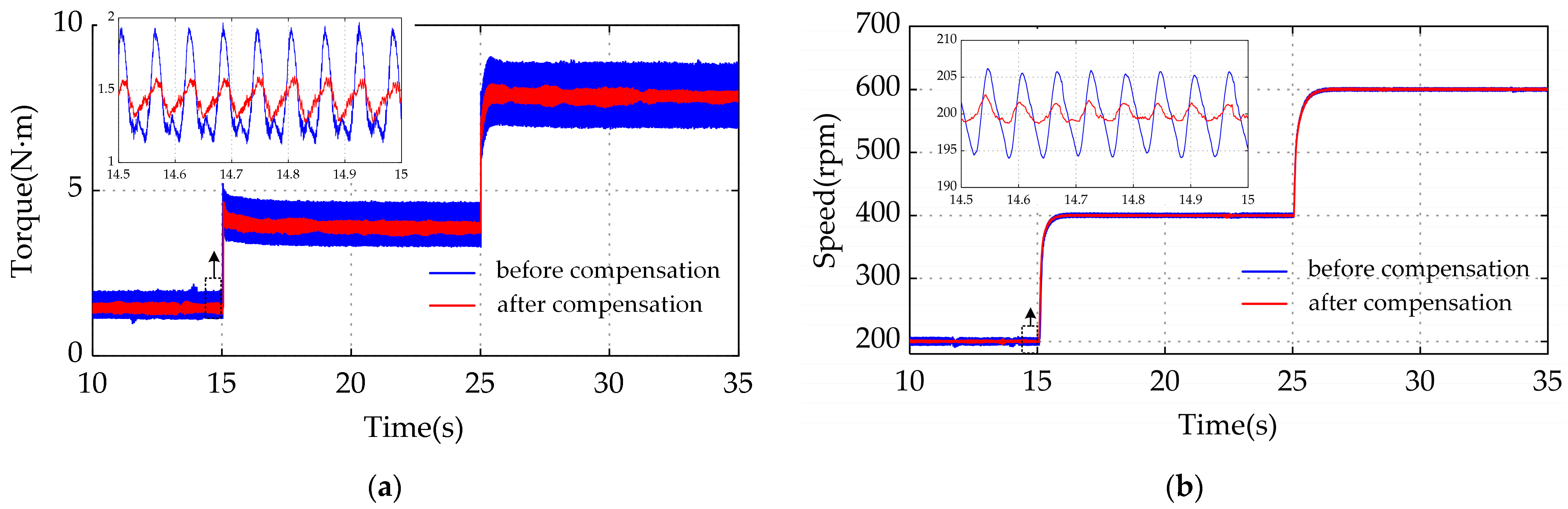
4.3. Dynamic Performance

To verify the dynamic performance, torque step and speed step experiments are performed. Figure 17 shows the comparison of experimental results with a torque step at different operating speeds. Figure 17a depicts the speed, the d-axes currents, and the torque at 600 rpm, while Figure 17b shows those at 360 rpm. It can be observed that the speed decreases due to the sudden load and then returns to the reference speed within 0.5 s. The torque rapidly increases by 1.2 N·m following the given value. The compensating strategy remains effective as torque increases.

Figure 18 shows the comparison results of the speed rising from 360 rpm to 600 rpm. With the proposed compensating strategy, the speed ripple and the torque ripple are effectively suppressed after a speed step. The speed can reach the desired speed in 0.5 s, which is essentially the same as the situation without compensation. Figure 17 and Figure 18 demonstrate that the proposed compensating strategy is always effective during the transient state. Moreover, the proposed compensation method has no impact on the dynamic performance of the motor.

To validate the efficacy of the proposed method, suppression effects of a single SOGI, the SOGI₂ (two SOGIs in series), and the cascade decoupling SOGIs on speed and q-axis current pulsations are experimentally compared. The results are shown in Figure 19, which demonstrate that the cascade decoupling SOGIs have the fastest convergence speed and the smallest fluctuations in motor speed and current utilizing the compensation method.

4.4. Comparison with Resonant Control in Ref. [15]

Resonant control, as mentioned in the introduction, has the capability to mitigate speed ripple by amplifying the gain of the speed loop at the disturbance frequency [15]. However, this method only improves the performance of the speed and the q-axis current and cannot compensate for the d-axis current. So, the phase currents still distort due to the incomplete compensation for the dq-axes current.

The first figure in Figure 20 shows the waveform for suppressing speed harmonics using the method described in Ref. [15]; the second figure shows the phase current of the motor without the compensation method, which exhibits obvious imbalance. The third and fourth figures depict the phase current waveforms after implementing the literature method and the proposed method, respectively. It can be seen that resonant control effectively suppresses speed ripple when measurement errors are introduced. The phase current harmonics are reduced slightly compared to those without compensation. By applying Fourier analysis, the total harmonic distortion decreases from 4.87% to 2.52%. However, the phase currents still exhibit significant imbalance. The last picture depicts the phase current using the proposed method. The total harmonic distortion is 1.68%, and there is essentially no phase current asymmetry. The reason is that the literature method cannot compensate for the harmonic component in the d-axis current, while the proposed method can simultaneously compensate for the harmonics in the dq-axes. Therefore, the method described in this paper effectively solves the problem of current measurement errors.

4.5. Experiments under Ship Propeller Load

Ref. [45] proposes a programmable dynamometer for simulating rotating loads that can accurately track the required torque–speed. Thus, the electrical load simulator (ELS) [46] is widely utilized for simulating the load torque of mechanical equipment and testing its performance indicators. It plays a key role in various fields, including aerospace [47], wind energy systems [48,49], ship electric propulsion systems [6,50,51,52], etc. Compared to traditional loading methods such as magnetic powder brakes and electro-hydraulic passive torque servo systems [53], this method offers shorter loading delays and higher torque accuracy, and is less affected by factors such as temperature changes. Consequently, this study employs an ELS to simulate propeller torque. In the experimental setup of this paper, both the power motor and the load motor are of the same motor. The power motor functions in speed control mode, while the load motor functions in torque control mode.

According to Refs. [6,54], the mathematical model for ship propeller load is depicted in Figure 21.

Table 5. Parameters of the propeller load model.

Parameters	Value
Hull mass Ms/kg	14
Mass of the attached water Δm/kg	1
Propeller diameter D/m	0.15
Thrust deduction coefficient t	0.08
Wake coefficient w	0.15

lists the parameters of the ship propeller model. The propeller load model can then be established in MATLAB/Simulink. Subsequently, the propeller torque can be calculated to control the load motor. The servo motor has a smaller loading delay and higher loading accuracy, which allows for better simulation of propeller load characteristics. Therefore, this paper utilizes the experimental platform to validate the efficacy of the suggested method in extracting and compensating for current measurement errors.

In Figure 21, L represents the propeller advance ratio, v_p represents the velocity of the propeller relative to water, measured in m/s, n represents the propeller rotation speed, measured in r/s, and D represents the diameter of the propeller measured in meters. K_p represents the dimensionless coefficient of propeller thrust, while K_T denotes the dimensionless coefficient of drag torque. These coefficients are dependent on the advance ratio L (Equation (24)). T_P represents the propeller torque, measured in N·m, P_e represents the thrust generated by rotation of the propeller, measured in N, t represents the thrust derating coefficient, and ρ is seawater density, typically 1025 kg/m³. m is the hull mass, and Δm represents the mass of attached water, typically estimated to be 5–15% of the hull’s mass. R_s is the ship’s total resistance, measured in N·m, which is a function of ship speed v_s [54] (Equation (25)). w is the measure of wake effects.

$$\left\{\begin{array}{l}{K}_{\mathrm{p}}=4.789-2.342L-1.501L^2\\ K_{\mathrm{T}}=1.897-0.541L-0.268L^2\end{array}\right.$$

(24)

$$R_{\mathrm{s}}=0.2951v_{\mathrm{s}}+ 0.5634v_{\mathrm{s}}\left|v_{\mathrm{s}}\right|$$

(25)

This paper primarily focuses on designing the harmonic extractor and compensator to address the problem of current sensor measurement errors in shipboard propulsion motors. The proposed method aims to suppress the first-order and second-order harmonics in the currents and rotational speed, thereby reducing the motor torque and rotational speed pulsations. This, in turn, reduces motor vibration and noise, ultimately improving the efficiency of the motor. The results are depicted in Figure 22, Figure 23 and Figure 24.

In Figure 22, the speed references are 200 rpm at t = 0 s, 400 rpm at t = 15 s, and 600 rpm at t = 25 s. As shown in Figure 22a, when there are current measurement errors, the amplitude of electromagnetic torque fluctuation is 0.78 N·m before compensation. However, it is reduced to 0.26 N·m after compensation. Correspondingly, the speed fluctuation before compensation is 12 rpm in Figure 22b, while it is 3.5 rpm after compensation. The speed pulsation rate is reduced from ±6% to ±0.875%, which complies with China’s national standard GB/T 35701-2017 [55].

The results of the FFT analysis of the waveforms depicted in Figure 22 are presented in

Table 6. FFT analysis results of Figure 22.

Harmonic Content		Torque (N·m)	Speed (rpm)
Before compensation	dc	1.4311	199.9
	1st	0.3063	5.42
	2nd	0.1622	1.12
	THD	24.13%	2.78%
After compensation	dc	1.4410	199.9
	1st	0.0947	1.02
	2nd	0.0330	0.28
	THD	6.78%	0.54%

, which shows that after compensation, the THD of the electromagnetic torque and speed are reduced by 71.9% and 80.5%, respectively. The experimental results show that there are significant reductions in the first-order and second-order harmonic content of torque and speed, and the total harmonic distortions of them are also greatly improved, which confirms that the compensation method can effectively enhance the quality of motor torque and reduce speed pulsation.

According to Figure 23 and Equation (24), variations in motor speed result in fluctuations in propeller torque, which subsequently leads to fluctuations in ship speed (with less impact). In Figure 23a, the propeller torque ripples are reduced by approximately 70%, from 0.22 N·m to 0.03 N·m. In Figure 23b, the results show that the compensation method has no impact on the ship’s acceleration performance. Additionally, it reduces propeller torque and ship speed pulsations.

Figure 24 shows the comparison of the phase current experimental results before and after compensation, and the corresponding FFT analysis results are shown in

Table 7. FFT analysis results of Figure 24.

Harmonic Content		Phase Current A (%)	Phase Current B (%)
Before compensation	dc	10.1	10.7
	2nd	3.5	3.6
	3rd	1.3	2.3
After compensation	dc	1.1	2.3
	2nd	0.1	0.3
	3rd	0.3	0.4

. It can be clearly seen that the phase current imbalance and harmonic distortion caused by current measurement errors have been significantly improved. In conclusion, the experimental results demonstrate that this algorithm is capable of effectively reducing the current and speed ripples of the propulsion motor and has a satisfactory control performance in both steady and transient states, which is suitable for complex marine environments.

4.6. HIL Test Result

To demonstrate the effectiveness of the proposed method in the application of a higher power shipboard permanent magnet propulsion motor variable frequency drive system, the motor parameters of a different electric propulsion vessel, as presented in

Table 8. Parameters of the electrical propulsion system in simulation.

Parameters	Value
Pole pairs	12
Stator resistance (Ω)	0.011
Stator inductor (H)	3.074 × 10−5
Flux (Wb)	0.3051
Moment of inertia (kg·m2)	0.8051
Rated power (kW)	100
Hull mass Ms/kg	31,000
Mass of the attached water Δm/kg	2000
Propeller diameter D/m	0.9
Thrust deduction coefficient t	0.13
Wake coefficient w	0.15

, are employed for hardware-in-the-loop (HIL) verification. The vessel measures 21.1 m in total length, has an empty weight of 29 metric tons, and is fitted with an AC propulsion motor rated at 100 kilowatts. The current measurement errors are described by Equation (26), and the examination pertains to the parameters of the electric propulsion vessel as delineated in Table 8.

$$\begin{array}{l}\mathsf{\Delta }{i}_{A\_\mathrm{offset}}=0.5\mathrm{A} K_A=0.9\\ \mathsf{\Delta }{i}_{B\_\mathrm{offset}}=-0.6\mathrm{A} K_B=1.1\end{array}$$

(26)

$$\left\{\begin{array}{l}{K}_{\mathrm{p}}=0.348-0.276L-0.168L^2\\ K_{\mathrm{T}}=0.0742-0.048L-0.0431L^2\end{array}\right.$$

(27)

$$R_{\mathrm{s}}=312.7v_{\mathrm{s}}\left|v_{\mathrm{s}}\right|$$

(28)

This article uses the high-performance product NIPXIE-1071 (Modeling Tech Energy Technology Co., Ltd., Shanghai, China) for hardware-in-the-loop testing. HIL testing uses simulation and modeling technology to verify advanced algorithms for ship trajectory tracking control [56], ship medium-voltage DC systems [57], and ship electric propulsion systems [58] to reduce testing duration and enhance coverage, particularly for test cases that are challenging to replicate consistently in a physical laboratory.

The HIL control structure is shown in Figure 25. The core components include a real-time hardware emulator based on the FPGA and a rapid control prototype (RCP) algorithm controller. RCP uses an Intel i7 quad-core processor, which is mainly responsible for controlling the implementation of algorithms, including the reception of feedback signals and the output of control signals. The real-time simulator is mainly responsible for the real-time simulation of crucial components, such as motor, encoder, capacitance, and switching devices, controlled by the RCP controller. It can output feedback variables to the RCP and interface panel for controller signal collection and oscilloscope observation. Computers can directly communicate with the HIL through Ethernet communication, download emulators, and observe real-time state variables.

Figure 26 and Figure 27 are test results sampled using Yokogawa’s DLM3024 (Yokogawa Co., Ltd., Tokyo, Japan). Figure 26a shows the measured speed of the propulsion motor at different given speeds. The speed fluctuation measured using the HIL platform is about 5 rpm. This is mainly caused by the inverter dead-zone effect and high-frequency noise of power electronic devices. Figure 26b shows the q-axis current at different speeds when the proposed method is not used. And it shows that as the motor speed increases to 600 rpm, the pulsation value of the q-axis current exceeds 10 A. Figure 26c shows the q-axis current at different speeds after using the proposed method. And it shows that the q-axis current ripple value drops to about 2.6 A at different speeds.

Figure 27a shows the phase current waveforms at different speeds before eliminating the current measurement errors with the proposed method. It can be seen from the amplified current waveform that the phase currents are obviously unbalanced at this time, and the peak-to-peak value of the two-phase current differs by about 8 A. Figure 27b shows that after using the proposed method to eliminate the current measurement errors, the phase current peak-to-peak error is reduced to about 1 A. The results obtained from the HIL platform comprehensively demonstrate that the proposed method is effective in variable drive systems for high-power motors.

5. Conclusions

A new strategy is proposed in this paper to simultaneously compensate for the harmonics in the dq-axes current in the vector control system of a ship’s propulsion motor. The current harmonics are accurately extracted by the cascade decoupling SOGIs and compensated by ADALINE compensators. Hence, the method effectively suppresses speed and electromagnetic torque ripples and also improves the distortion of phase currents. This method requires no additional hardware and is not reliant on motor parameters. Furthermore, the compensatory parameters are self-tuning, utilizing the advantages of the ADALINE network. The verifications of this method are as follows.

(1) Experiments are conducted on the PMSM drive system, and the results demonstrate that the control strategy exhibits excellent steady-state and transient-state performance. Additionally, the first-order and second-order ripple components of the motor’s electromagnetic torque are reduced from 0.3035 N·m to 0.1341 N·m and from 0.3171 N·m to 0.0634 N·m, respectively. When used as a ship propulsion motor, the electromagnetic torque’s first-order and second-order harmonic components are decreased from 0.3063 N·m to 0.0947 N·m and from 0.1623 N·m to 0.033 N·m, respectively. Meanwhile, the harmonic components of the speed are reduced from 5.42 rpm to 1.02 rpm and from 1.02 rpm to 0.28 rpm, respectively. Additionally, the A-phase current’s dc and second-order harmonic components are reduced from 10.1% to 1.1% and from 3.5% to 0.1%, respectively.

(2) The supplementary hardware-in-the-Loop (HIL) test on the 100 kW propulsion motor validates the effectiveness of this method in mitigating the impact of current measurement errors. This is demonstrated by the decrease in the q-axis current ripple from 10.5 A to 2.6 A at 600 rpm, as well as an 85% reduction in phase current imbalance.

Future research will focus on reducing the algorithm’s complexity, simplifying the compensation structure, and validating the efficacy of the proposed algorithm for sensorless control of propulsion motors. These adjustments will make the algorithm suitable for a wider range of control situations.

References

1. Haxhiu, A.; Abdelhakim, A.; Kanerva, S.; Bogen, J. Electric Power Integration Schemes of the Hybrid Fuel Cells and Batteries-Fed Marine Vessels-An Overview. IEEE Trans. Transp. Electrif. 2022, 8, 1885–1905. [Google Scholar] [CrossRef]
2. Bai, H.; Yu, B.; Gu, W. Research on Position Sensorless Control of RDT Motor Based on Improved SMO with Continuous Hy-perbolic Tangent Function and Improved Feedforward PLL. J. Mar. Sci. Eng. 2023, 11, 642. [Google Scholar] [CrossRef]
3. Qin, J.; Du, J. Robust adaptive asymptotic trajectory tracking control for underactuated surface vessels subject to unknown dynamics and input saturation. J. Mar. Sci. Technol. 2022, 27, 307–319. [Google Scholar] [CrossRef]
4. Gu, N.; Wang, D.; Peng, Z.H.; Wang, J. Safety-Critical Containment Maneuvering of Underactuated Autonomous Surface Vehicles Based on Neurodynamic Optimization With Control Barrier Functions. IEEE Trans. Neural Netw. Learn. Syst. 2023, 34, 2882–2895. [Google Scholar] [CrossRef]
5. Guo, H.; Xiang, T.; Liu, Y.; Zhang, Q.; Liu, S.; Guan, B. Active Disturbance Rejection Control Method for Marine Permanent-Magnet Propulsion Motor Based on Improved ESO and Nonlinear Switching Function. J. Mar. Sci. Eng. 2023, 11, 1751. [Google Scholar] [CrossRef]
6. Ren, J.-J.; Liu, Y.-C.; Wang, N.; Liu, S.-Y. Sensorless control of ship propulsion interior permanent magnet synchronous motor based on a new sliding mode observer. ISA Trans. 2015, 54, 15–26. [Google Scholar] [CrossRef]
7. Hu, M.; Hua, W.; Wu, Z.; Dai, N.; Xiao, H.; Wang, W. Compensation of Current Measurement Offset Error for Permanent Magnet Synchronous Machines. IEEE Trans. Power Electron. 2020, 35, 11119–11128. [Google Scholar] [CrossRef]
8. Cho, K.-R.; Seok, J.-K. Correction on current measurement errors for accurate flux estimation of AC drives at low stator frequency. IEEE Trans. Ind. Appl. 2008, 44, 594–603. [Google Scholar] [CrossRef]
9. Chung, D.W.; Sul, S.K. Analysis and compensation of current measurement error in vector-controlled AC motor drives. IEEE Trans. Ind. Appl. 1998, 34, 340–345. [Google Scholar] [CrossRef]
10. Chuan, H.; Fazeli, S.M.; Wu, Z.; Burke, R. Mitigating the Torque Ripple in Electric Traction Using Proportional Integral Resonant Controller. IEEE Trans. Veh. Technol. 2020, 69, 10820–10831. [Google Scholar] [CrossRef]
11. Han, J.; Kim, B.-H.; Sui, S.-k. Effect of Current Measurement Error in Angle Estimation of Permanent Magnet AC Motor Sensorless Control. In Proceedings of the 3rd IEEE International Future Energy Electronics Conference/Energy Conversion Congress and Exposition (ECCE) Asia, Taiwan, China, 4–7 June 2017; pp. 2171–2176. [Google Scholar]
12. Choi, C.-H.; Cho, K.-R.; Seok, J.-K. Inverter nonlinearity compensation in the presence of current measurement errors and switching device parameter uncertainties. IEEE Trans. Power Electron. 2007, 22, 576–583. [Google Scholar] [CrossRef]
13. Shen, Z.; Jiang, D. Dead-Time Effect Compensation Method Based on Current Ripple Prediction for Voltage-Source Inverters. IEEE Trans. Power Electron. 2019, 34, 971–983. [Google Scholar] [CrossRef]
14. Myers, G.P.; Degner, M.W. Compensation Method for Current-Sensor Gain Error. U.S. Patent 6,998,811, 14 February 2006. [Google Scholar]
15. Zhang, Q.; Guo, H.; Guo, C.; Liu, Y.; Wang, D.; Lu, K.; Zhang, Z.; Zhuang, X.; Chen, D. An adaptive proportional-integral-resonant controller for speed ripple suppression of PMSM drive due to current measurement error. Int. J. Electr. Power Energy Syst. 2021, 129, 106866. [Google Scholar] [CrossRef]
16. Zhou, Z.; Xia, C.; Yan, Y.; Wang, Z.; Shi, T. Disturbances Attenuation of Permanent Magnet Synchronous Motor Drives Using Cascaded Predictive-Integral-Resonant Controllers. IEEE Trans. Power Electron. 2018, 33, 1514–1527. [Google Scholar] [CrossRef]
17. Xia, C.; Ji, B.; Yan, Y. Smooth Speed Control for Low-Speed High-Torque Permanent-Magnet Synchronous Motor Using Proportional-Integral-Resonant Controller. IEEE Trans. Ind. Electron. 2015, 62, 2123–2134. [Google Scholar] [CrossRef]
18. Zhang, Q.; Guo, H.; Liu, Y.; Guo, C.; Lu, K.; Wang, D.; Zhang, Z.; Sun, J. Robust plug-in repetitive control for speed smoothness of cascaded-PI PMSM drive. Mech. Syst. Signal Proc. 2022, 163, 108090. [Google Scholar] [CrossRef]
19. Tang, M.; Gaeta, A.; Formentini, A.; Zanchetta, P. A Fractional Delay Variable Frequency Repetitive Control for Torque Ripple Reduction in PMSMs. IEEE Trans. Ind. Appl. 2017, 53, 5553–5562. [Google Scholar] [CrossRef]
20. Tang, M.; Formentini, A.; Odhano, S.A.; Zanchetta, P. Torque Ripple Reduction of PMSMs Using a Novel Angle-Based Repetitive Observer. IEEE Trans. Ind. Electron. 2020, 67, 2689–2699. [Google Scholar] [CrossRef]
21. Liu, J.; Li, H.; Deng, Y. Torque Ripple Minimization of PMSM Based on Robust ILC Via Adaptive Sliding Mode Control. IEEE Trans. Power Electron. 2018, 33, 3655–3671. [Google Scholar] [CrossRef]
22. Qian, W.; Panda, S.K.; Xu, J.X. Speed ripple minimization in PM synchronous motor using iterative learning control. IEEE Trans. Energy Convers. 2005, 20, 53–61. [Google Scholar] [CrossRef]
23. Lee, K.-W.; Kim, S.-I. Dynamic Performance Improvement of a Current Offset Error Compensator in Current Vector-Controlled SPMSM Drives. IEEE Trans. Ind. Electron. 2019, 66, 6727–6736. [Google Scholar] [CrossRef]
24. Harke, M.C.; Guerrero, J.M.; Degner, M.W.; Briz, F.; Lorenz, R.D. Current measurement gain tuning using high-frequency signal injection. IEEE Trans. Ind. Appl. 2008, 44, 1578–1586. [Google Scholar] [CrossRef]
25. Jung, H.-S.; Hwang, S.-H.; Kim, J.-M.; Kim, C.-U.; Choi, C. Diminution of current-measurement error for vector-controlled ac motor drives. IEEE Trans. Ind. Appl. 2006, 42, 1249–1256. [Google Scholar] [CrossRef]
26. Kim, M.; Sul, S.-K.; Lee, J. Compensation of Current Measurement Error for Current-Controlled PMSM Drives. IEEE Trans. Ind. Appl. 2014, 50, 3365–3373. [Google Scholar] [CrossRef]
27. Ciobotaru, M.; Teodorescu, R.; Blaabjerg, F. A new single-phase PLL structure based on second order generalized integrator. In Proceedings of the 37th IEEE Power Electronics Specialist Conference (PESC 2006), Cheju Island, Republic of Korea, 18–22 June 2006; pp. 1–6. [Google Scholar]
28. Rodriguez, P.; Luna, A.; Candela, I.; Mujal, R.; Teodorescu, R.; Blaabjerg, F. Multiresonant Frequency-Locked Loop for Grid Synchronization of Power Converters Under Distorted Grid Conditions. IEEE Trans. Ind. Electron. 2011, 58, 127–138. [Google Scholar] [CrossRef]
29. Matas, J.; Castilla, M.; Miret, J.; Garcia de Vicuna, L.; Guzman, R. An Adaptive Prefiltering Method to Improve the Speed/Accuracy Tradeoff of Voltage Sequence Detection Methods Under Adverse Grid Conditions. IEEE Trans. Ind. Electron. 2014, 61, 2139–2151. [Google Scholar] [CrossRef]
30. Wang, G.; Ding, L.; Li, Z.; Xu, J.; Zhang, G.; Zhan, H.; Ni, R.; Xu, D. Enhanced Position Observer Using Second-Order Generalized Integrator for Sensorless Interior Permanent Magnet Synchronous Motor Drives. IEEE Trans. Energy Convers. 2014, 29, 486–495. [Google Scholar] [CrossRef]
31. Liu, B.; Zhou, B.; Ni, T. Principle and Stability Analysis of an Improved Self-Sensing Control Strategy for Surface-Mounted PMSM Drives Using Second-Order Generalized Integrators. IEEE Trans. Energy Convers. 2018, 33, 126–136. [Google Scholar] [CrossRef]
32. Xu, W.; Jiang, Y.; Mu, C.; Blaabjerg, F. Improved Nonlinear Flux Observer-Based Second-Order SOIFO for PMSM Sensorless Control. IEEE Trans. Power Electron. 2019, 34, 565–579. [Google Scholar] [CrossRef]
33. Zhao, R.; Xin, Z.; Loh, P.C.; Blaabjerg, F. A Novel Flux Estimator Based on Multiple Second-Order Generalized Integrators and Frequency-Locked Loop for Induction Motor Drives. IEEE Trans. Power Electron. 2017, 32, 6286–6296. [Google Scholar] [CrossRef]
34. Xin, Z.; Zhao, R.; Blaabjerg, F.; Zhang, L.; Loh, P.C. An Improved Flux Observer for Field-Oriented Control of Induction Motors Based on Dual Second-Order Generalized Integrator Frequency- Locked Loop. IEEE J. Emerg. Sel. Top. Power Electron. 2017, 5, 513–525. [Google Scholar] [CrossRef]
35. Yoo, J.; Kim, H.-S.; Sul, S.-K. Design of Frequency-Adaptive Flux Observer in PMSM Drives Robust to Discretization Error. IEEE Trans. Ind. Electron. 2022, 69, 3334–3344. [Google Scholar] [CrossRef]
36. Zhang, Q.; Guo, H.; Liu, Y.; Guo, C.; Zhang, F.; Zhang, Z.; Li, G. A Novel Error-Injected Solution for Compensation of Current Measurement Errors in PMSM Drive. IEEE Trans. Ind. Electron. 2023, 70, 4608–4619. [Google Scholar] [CrossRef]
37. Zhu, H.; Fujimoto, H. Suppression of Current Quantization Effects for Precise Current Control of SPMSM Using Dithering Techniques and Kalman Filter. IEEE Trans. Ind. Inform. 2014, 10, 1361–1371. [Google Scholar] [CrossRef]
38. Asiminciaei, L.; Blaabjerg, F.; Hansen, S. Detection is key—Harmonic detection methods for active power filter applications. IEEE Ind. Appl. Mag. 2007, 13, 22–33. [Google Scholar] [CrossRef]
39. Xin, Z.; Wang, X.; Qin, Z.; Lu, M.; Loh, P.C.; Blaabjerg, F. An Improved Second-Order Generalized Integrator Based Quadrature Signal Generator. IEEE Trans. Power Electron. 2016, 31, 8068–8073. [Google Scholar] [CrossRef]
40. Wang, L.; Zhu, Z.Q.; Bin, H.; Gong, L. A Commutation Error Compensation Strategy for High-Speed Brushless DC Drive Based on Adaline Filter. IEEE Trans. Ind. Electron. 2021, 68, 3728–3738. [Google Scholar] [CrossRef]
41. Tang, Z.; Akin, B. A New LMS Algorithm Based Deadtime Compensation Method for PMSM FOC Drives. IEEE Trans. Ind. Appl. 2018, 54, 6472–6484. [Google Scholar] [CrossRef]
42. Qasim, M.; Kanjiya, P.; Khadkikar, V. Optimal Current Harmonic Extractor Based on Unified ADALINEs for Shunt Active Power Filters. IEEE Trans. Power Electron. 2014, 29, 6383–6393. [Google Scholar] [CrossRef]
43. Ni, K.; Gan, C.; Peng, G.; Shi, H.; Hu, Y.; Qu, R. Power Compensation-Oriented SVM-DPC Strategy for a Fault-Tolerant Back-to-Back Power Converter Based DFIM Shipboard Propulsion System. IEEE Trans. Ind. Electron. 2022, 69, 8716–8726. [Google Scholar] [CrossRef]
44. Ni, K.; Gan, C.; Peng, G.; Hu, Y.; Qu, R. Impedance-Based Stability Analysis of Less Power Electronics Integrated Electric Shipboard Propulsion System Considering Operation Mode, PLL, and DC-Bus Voltage Control Effect. IEEE Trans. Veh. Technol. 2021, 70, 2219–2230. [Google Scholar] [CrossRef]
45. Collins, E.R.; Huang, Y. A programmable dynamometer for testing rotating machinery using a three-phase induction machine. IEEE Trans. Energy Convers. 1994, 9, 521–527. [Google Scholar] [CrossRef]
46. Wang, L.; Wang, M.; Guo, B.; Wang, Z.; Wang, D.; Li, Y. Analysis and Design of a Speed Controller for Electric Load Simulators. IEEE Trans. Ind. Electron. 2016, 63, 7413–7422. [Google Scholar] [CrossRef]
47. Nam, Y. QFT force loop design for the aerodynamic load simulator. IEEE Trans. Aerosp. Electron. Syst. 2001, 37, 1384–1392. [Google Scholar] [CrossRef]
48. Kojabadi, H.M.; Chang, L.C.; Boutot, T. Development of a novel wind turbine simulator for wind energy conversion systems using an inverter-controlled induction motor. IEEE Trans. Energy Convers. 2004, 19, 547–552. [Google Scholar] [CrossRef]
49. Li, H.; Steurer, M.; Shi, K.L.; Woodruff, S.; Zhang, D. Development of a unified design, test, and research platform for wind energy systems based on hardware-in-the-loop real-time simulation. IEEE Trans. Ind. Electron. 2006, 53, 1144–1151. [Google Scholar] [CrossRef]
50. Zhang, Z.; Guo, H.; Liu, Y.; Zhang, Q.; Zhu, P.; Iqbal, R. An Improved Sensorless Control Strategy of Ship IPMSM at Full Speed Range. IEEE Access 2019, 7, 178652–178661. [Google Scholar] [CrossRef]
51. Aidi, S.; Hui, H.; Wei, K. Marine AC high-capacity drive experiment system. In Proceedings of the 2010 International Conference on Computer, Mechatronics, Control and Electronic Engineering, Changchun, China, 24–26 August 2010; pp. 33–36. [Google Scholar]
52. Huang, H.; Shen, A.-D.; Chu, J.-X. Research on propeller dynamic load simulation system of electric propulsion ship. China Ocean Eng. 2013, 27, 255–263. [Google Scholar] [CrossRef]
53. Zheng, D.; Xu, H. Modeling and high accuracy parameter estimates for a friction based electro-hydraulic load simulator. In Proceedings of the 2016 IEEE International Conference on Mechatronics and Automation, Harbin, China, 7–10 August 2016; pp. 2392–2397. [Google Scholar]
54. Fossen, T.I.; Blanke, M. Nonlinear output feedback control of underwater vehicle propellers using feedback form estimated axial flow velocity. IEEE J. Ocean. Eng. 2000, 25, 241–255. [Google Scholar] [CrossRef]
55. GB/T 35701-2017; Marine Converter of Electric Propulsion. Chinese National Standard: Beijing, China, 2017; pp. 1–13.
56. Sivaraman, S.; Awanish, D.; Suresh, R. On the performance of different Deep Reinforcement Learning based controllers for the path-following of a ship. Ocean Eng. 2023, 286, 115607. [Google Scholar] [CrossRef]
57. Yang, G.; Xiao, F.; Fan, X.; Wang, R.; Liu, J. Three-Phase Three-Level Phase-Shifted PWM DC–DC Converter for Electric Ship MVDC Application. IEEE J. Emerg. Sel. Top. Power Electron. 2017, 5, 162–170. [Google Scholar] [CrossRef]
58. Dufour, C.; Dumur, G.; Paquin, J.N.; Belanger, J. A PC-based hardware-in-the-loop simulator for the integration testing of modern train and ship propulsion systems. In Proceedings of the 2008 IEEE Power Electronics Specialists Conference, Rhodes, Greece, 15–19 June 2008; pp. 444–449. [Google Scholar] [CrossRef]
Figure 1. Distribution diagram of current measurement errors in the vector control system of a ship’s permanent magnet propulsion motor.
Jmse 12 00154 g001
Figure 2. Control block diagram with proposed harmonic compensation strategy.
Jmse 12 00154 g002
Figure 3. Structure of second-order generalized integrator.
Jmse 12 00154 g003
Figure 4. Structure diagram of cascade decoupling SOGI.
Jmse 12 00154 g004
Figure 5. Amplitude–frequency characteristic comparison of single SOGI, SOGI2, and cascade decoupling SOGIs. (a) Output v1. (b) Output v2.
Jmse 12 00154 g005
Figure 6. Extracted harmonic comparison of single SOGI, SOGI2, and cascade decoupling SOGIs. (a) 30 Hz. (b) 60 Hz. (c) 180 Hz.
Jmse 12 00154 g006
Figure 7. Transfer function diagrams. (a) Standard first-order system (FOS). (b) Structures of SOGI drawn with generalized integrator (GI) transfer function.
Jmse 12 00154 g007
Figure 8. Step responses of SOS and SOGI2.
Jmse 12 00154 g008
Figure 9. Step responses of SOGI2 and SOGIs. (a) k = 0.3. (b) k = 1.414. (c) k = 3.
Jmse 12 00154 g009
Figure 10. Block diagram of dq-axes current ADALINE compensators.
Jmse 12 00154 g010
Figure 11. Amplitude–frequency characteristics of ADALINE compensators with different learning rates.
Jmse 12 00154 g011
Figure 12. Overall control block diagram of the proposed compensation structure.
Jmse 12 00154 g012
Figure 13. Experimental platform.
Jmse 12 00154 g013
Figure 14. Experimental results with different k and different η. (a) Different k. (b) Different η.
Jmse 12 00154 g014
Figure 15. Experimental results at 360 rpm. (a) Without compensation. (b) With compensation.
Jmse 12 00154 g015
Figure 16. Experimental results at 450 rpm.
Jmse 12 00154 g016
Figure 17. Comparison of experimental results of 1.2 N·m torque step with compensating strategy. (a) 600 rpm. (b) 360 rpm.
Jmse 12 00154 g017
Figure 18. Speed step comparison results (360 rpm to 600 rpm).
Jmse 12 00154 g018
Figure 19. Comparison results of speed and q-axis current among three SOGI structures. (a) Speed. (b) Current.
Jmse 12 00154 g019
Figure 20. Comparison results between the proposed method and resonant control in Ref. [15].
Jmse 12 00154 g020
Figure 21. Ship propeller load mathematical model.
Jmse 12 00154 g021
Figure 22. Comparison of experimental results before and after compensation. (a) Motor torque. (b) Speed.
Jmse 12 00154 g022
Figure 23. Comparison of experimental results before compensation and after compensation. (a) Propeller torque. (b) Ship speed.
Jmse 12 00154 g023
Figure 24. Comparison of phase current experimental results. (a) Before compensation. (b) After compensation.
Jmse 12 00154 g024
Figure 25. HIL hardware structure.
Jmse 12 00154 g025
Figure 26. Speed and q-axis current of HIL test. (a) Speed. (b) q-axis current before compensation. (c) q-axis current after compensation.
Jmse 12 00154 g026aJmse 12 00154 g026b
Figure 27. Phase currents of HIL test. (a) Before compensation. (b) After compensation.
Jmse 12 00154 g027aJmse 12 00154 g027b