UAV Path Planning for Container Terminal Yard Inspection in a Port Environment

Abstract

Container terminal yards are automated terminal yards. The rail-mounted gantry crane (RMGC) and rail-mounted gantry crane tracks (RMGCTs) that frequently operate in terminal yards need to be inspected regularly to ensure the safe operation of container transportation in the yard. This paper proposes a framework for the path planning of RMGCT visual inspection using a UAV in container terminal yards in a port environment. The framework consisted of two main aspects. First, a global path to all inspection viewpoints was planned according to the inspection requirements using the A* algorithm and the improved minimum snap method. Second, the intelligent bidirectional rapidly exploring random trees star (IB-RRT*) algorithm was introduced to plan the local path during the flight of the UAV. Finally, the feasibility of the path-planning framework was demonstrated using simulation experiments.

1. Introduction

The container terminal yard in a port environment is an automated yard. In the yard environment, rail-mounted gantry cranes (RMGCs) are critical to the picking and placing of containers [1]. However, due to the long-term exposure and frequent operation of RMGCs, rail-mounted gantry crane tracks (RMGCTs) are prone to wear, rust, cracks, and other damage. Therefore, the regular inspection of RMGCTs is crucial. However, the traditional method of manual inspection is subjective and inefficient. In recent years, unmanned aerial vehicles (UAVs) have been applied to the inspection of large equipment and power lines because of their high degree of freedom, maneuverability, and ability to carry various inspection equipment [2].

In scientific research and engineering applications, UAVs have attracted the attention of researchers due to their high maneuverability, good operation performance, and low cost. They have conducted in-depth research on path planning for UAVs. Regarding the problem of path planning, many researchers have given solutions, for example, the Dijkstra [3,4], A* [5,6], probabilistic road map (PRM) [7,8], and rapidly exploring random tree (RRT) [9,10,11] algorithms. Dijkstra and A*, which involve search-based pathfinding, can find the optimal path. They take a relatively long time to find the path, especially if the map is relatively large or in a three-dimensional environment. But they can be used in global path planning regardless of time constraints. The PRM and RRT algorithms are sampling-based path-planning algorithms, unlike the previous two algorithms (Dijkstra and A*). They all work by randomly generating a large number of points in the map and connecting these points through a simple local path planner or tree. But PRM is not widely used because of its low efficiency when finding the path. The RRT algorithm has higher efficiency than the PRM algorithm, where it can find a feasible but not optimal path in a shorter time. The RRT* algorithm [12] is one of the most significant variants of the RRT algorithm. Just like the RRT algorithm, RRT* can generate the initial path to the target rapidly. Although it can finally find an optimal path, it takes a long time to converge on the optimal solution. Based on the RRT* algorithm, a bidirectional version of RRT* was presented, which was named BI-RRT* [13]. BI-RRT* uses a slight variation of the greedy RRT-Connect heuristic for a connection with two trees [14], which can further reduce the time to find a feasible route each time. However, this method cannot guarantee the asymptotic optimality of each feasible route. To improve the superiority over the BI-RRT* algorithm, an intelligent bidirectional-RRT* (IB-RRT*) algorithm was proposed [15], which can reduce the planning time for each feasible path while ensuring the asymptotic optimality of each feasible path. With these dual advantages, the IB-RRT* algorithm has more efficient path-planning capability.

UAV trajectory planning is an important part of determining the UAV path after path planning. It optimizes the generated paths by considering the kinematic and dynamical constraints of the UAV so that the generated trajectories can be directly used for the flight of the UAV. The current UAV-trajectory-planning algorithms have been studied by a large number of scholars. The most common methods are the direct configuration method and the shooting method [16,17]. They can generate optimal local paths, but this is computationally intensive, relatively demanding on the environment, and rarely applied to practical UAV flight scenarios. 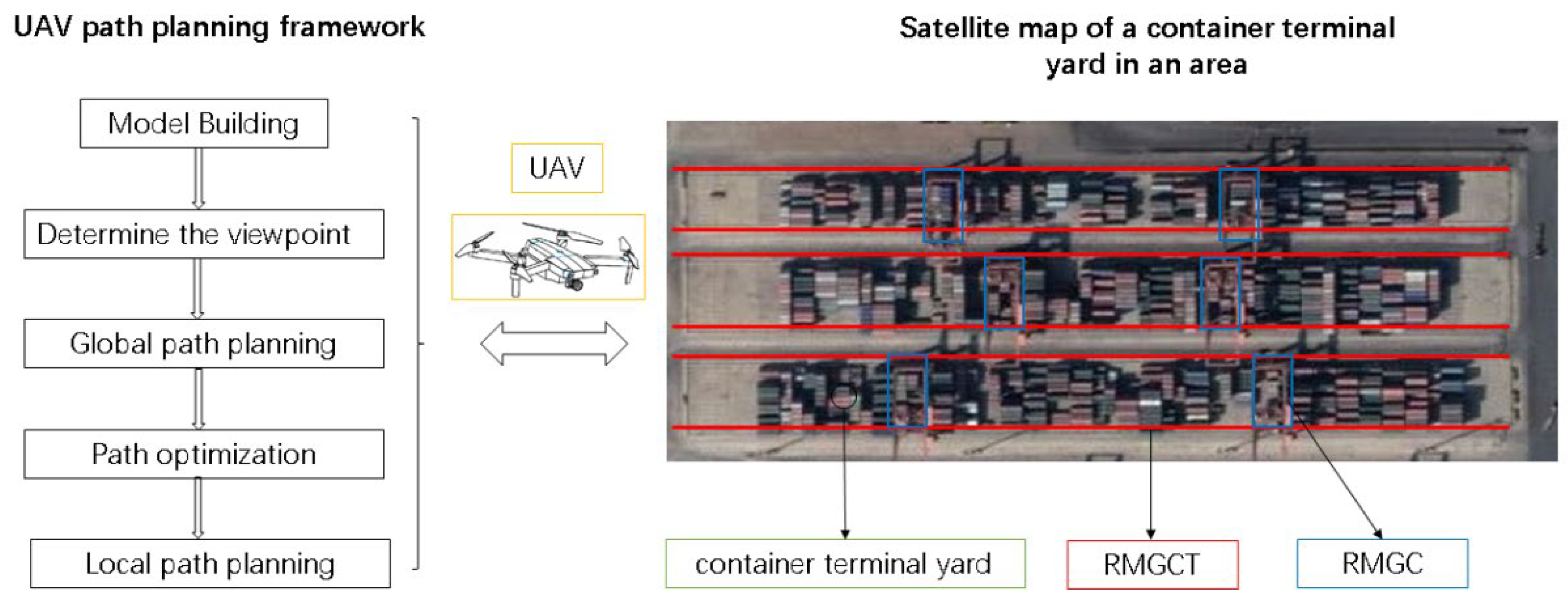Moreover, the most commonly used trajectory-planning algorithms include B-spline curves [18], Bezier curves [19], the K-trajectory algorithm [20], and the minimum snap algorithm [21,22]. The B-spline curve is suitable for the optimization of the initial path planned by the artificial potential field algorithm. The Bezier curve is suitable for the path optimization of a robotic arm. The K-trajectory algorithm is suitable for trajectory optimization in the presence of obstacles and narrow passages. In this study, the path of the UAV was optimized in the environment of a port container yard, and, thus, the above algorithms did not apply to the scenario of this study. The minimum snap method is suitable for the trajectory optimization of UAVs with high degrees of freedom, which can satisfy the constraints on the speed and acceleration of UAVs during flight; therefore, it is often used for UAV trajectory planning. However, a UAV trajectory planned by the original minimum snap method has a long length and large trajectory deviation, and, thus, needs to be improved, such as via geometric pre-processing. To improve the efficiency and accuracy of RMGCT inspections, this paper proposes a framework for path planning for the inspection of RMGCTs using a UAV. The framework consists of five main parts, as shown in Figure 1.

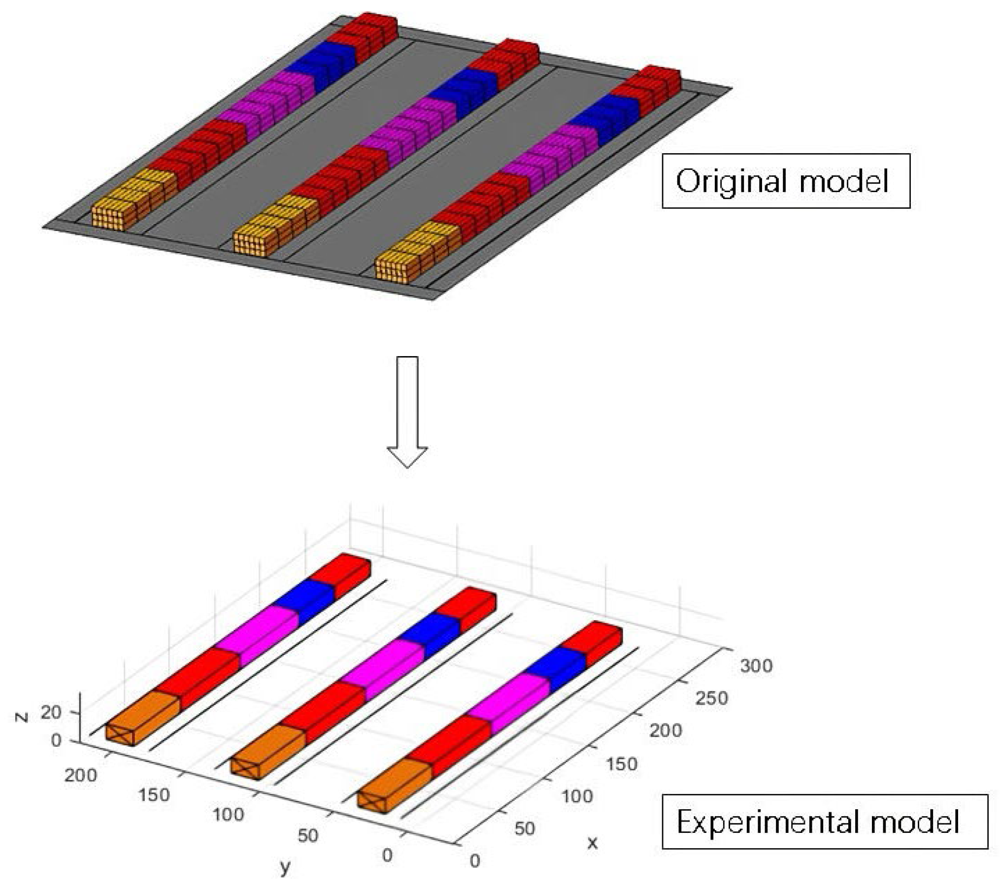
(1) Model building: In the initial phase of model building, a comprehensive representation of the container terminal yard (as shown in Figure 1) was synthesized, incorporating both the rail-mounted gantry crane terminals (RMGCTs) and the containers by integrating satellite imagery of the area.

(2) Determine the viewpoint: Upon the completion of the model, the determination of the viewpoint ensued. This stage was critical within the inspection protocol, as it significantly influenced the ultimate efficiency and efficacy of the inspection process. In this part, the detection viewpoint was determined according to the detection requirements and the parameters of the detection equipment carried by the UAV.

(3) Global path planning: After determining the appropriate viewpoint, the A* algorithm was used to plan the global path to all inspection viewpoints. This global path did not consider the constraints of man–machine kinematics and dynamics, and, thus, it cannot be used in real scenarios.

(4) Path optimization: In the third part of the framework, although the A* algorithm facilitated the establishment of a preliminary global path, it neglected the kinematic and dynamic constraints inherent to the UAV. Consequently, in this part, the minimum snap criterion was invoked to refine this global trajectory. However, the initial optimization via the minimum snap method yielded suboptimal results, prompting the implementation of geometric optimization. This additional refinement step is crucial for the synthesis of an enhanced global path that adheres more closely to the UAV’s operational capabilities.

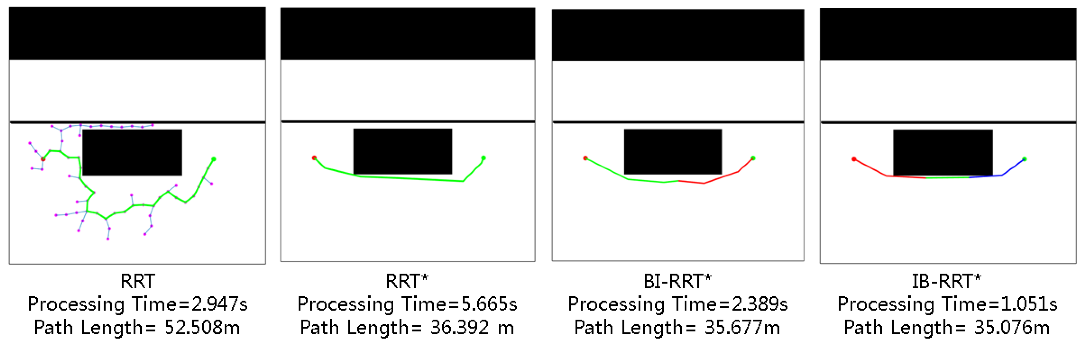
(5) Local path planning: Upon completion of the global path optimization, attention shifted to the execution of local path planning, a crucial step for circumventing static and dynamic obstacles in real-time. Within this context, a comparative analysis of the IB-RRT*, RRT*, and BI-RRT* algorithms was undertaken to ascertain their efficacy in this scenario. The IB-RRT* algorithm emerged as the preferred method for local path planning, owing to its superior performance in navigating the intricacies of the immediate operational environment.

The above method describes the framework for UAV inspection trajectories. This strategy improves the effectiveness of the inspection process, improving the economic benefits, and increases the safety and reliability of UAV inspection.

2. Problem Formulation

The objective of this paper is to find a path to all RMGCT inspection viewpoints. This inspection path should satisfy four main objectives: (1) avoiding all obstacles; (2) covering all viewpoints; (3) satisfying the flight constraints of the UAV; and (4) having the shortest possible flight time. First, this paper uses the A* algorithm and the improved minimum snap algorithm to plan a global path for UAV inspection through all viewpoints in a region. Second, the IB-RRT* algorithm is used for local path planning to avoid static real-time obstacles to UAV flight, such as trucks, during RMGC flight.

2.1. Description of Inspection

In recent years, inspection technology has been applied to various fields, such as the inspection of large buildings or mechanical equipment such as bridges and wind turbines. In the process of inspection, the UAV’s body, obstacle avoidance system, and control system and the inspection equipment carried have a great influence on the completion of the task. Among them, the body of the UAV serves as the carrier for various equipment and systems, and it is also the main body of mission execution. The purpose of the obstacle avoidance system is to avoid real-time obstacles to local path planning. Within this, the common equipment needed to avoid obstacles mainly includes lidar sensors and vision sensors. The control system mainly controls the UAV to fly along the designated path according to the planned global path and local path. The inspection equipment on board plays a very important role in the collection of inspection objects. Common inspection equipment includes lidar [23], infrared thermal imagers [24], high-resolution visible-light cameras [25], and so on. This article mainly collected images, so a high-resolution visible-light camera was selected as the inspection equipment. In addition, since the power supply of the UAV was not the main research focus of this paper, this paper was assumed to be finding a UAV path in an ideal scenario without considering the battery capacity.

2.2. Image Visual Inspection Description

In recent years, visual inspection technology has rapidly developed. In this paper, a UAV equipped with a high-resolution camera was used for image acquisition, and the collected images were used for visual inspection to finally obtain the inspection information for the inspection surface, which improved both the efficiency of image acquisition and the quality of defect inspection.

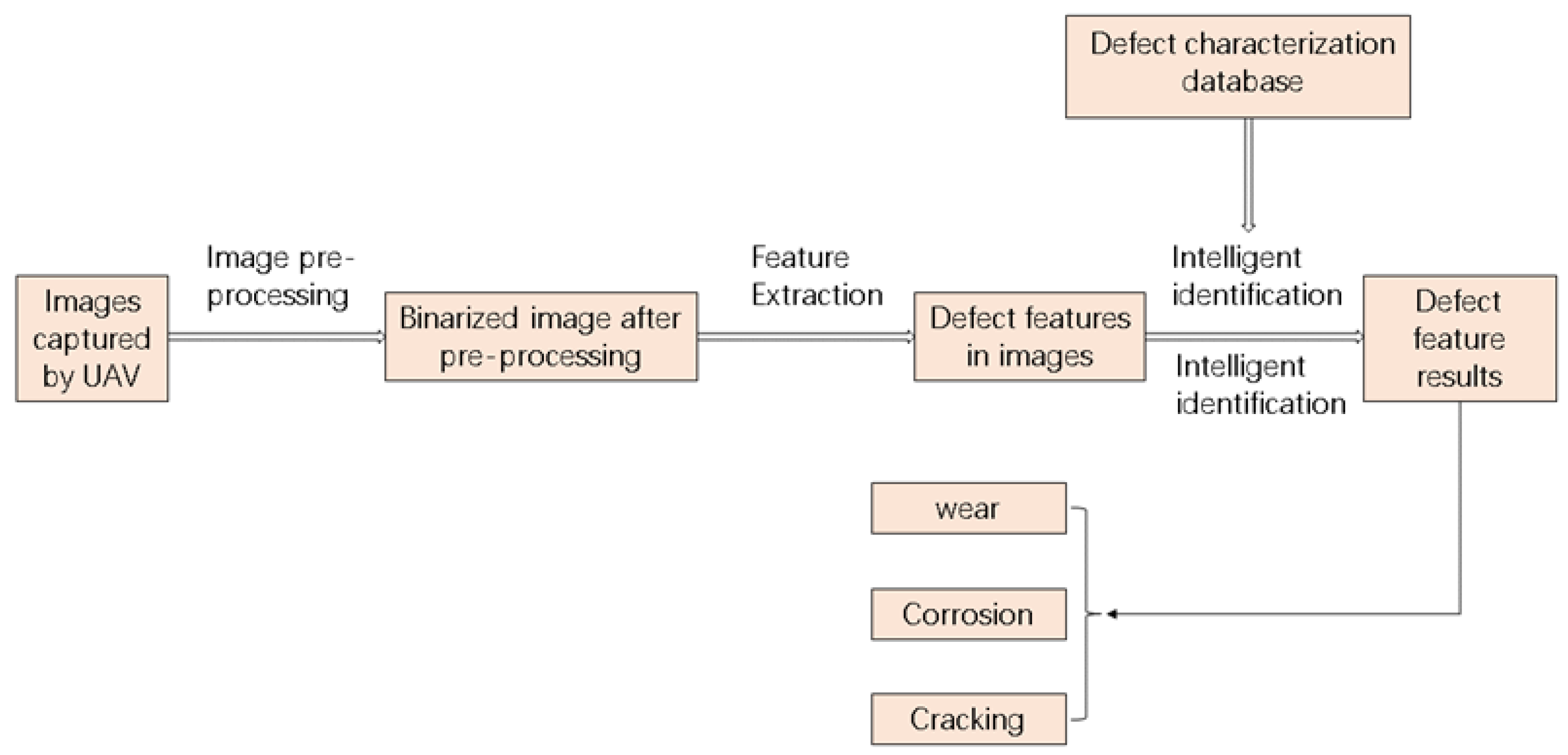
The steps of visual inspection are shown in Figure 2, which include acquisition image pre-processing, feature extraction, automatic defect inspection, and intelligent identification. Image pre-processing is mainly to solve the problems of noise interference, blurring, jitter, distortion, etc. in the images captured by the UAV and to binarize the images. Next, feature extraction is performed on the image after image pre-processing. The purpose of feature extraction is to extract the defect features in the image for subsequent defect inspection and intelligent recognition. Then, the extracted defect features are compared with the defect features in an image library to determine the defect types in the gantry crane tracks. The defect features in the image library represent the feature library that has been extracted and confirm the defect types. Through the above steps, this paper determines the defect locations and defect types in gantry cranes. The literature [26,27,28] provides a detailed description of visual inspection. This paper focuses on the trajectory planning method for the UAV. Therefore, the process of image acquisition will not be presented.

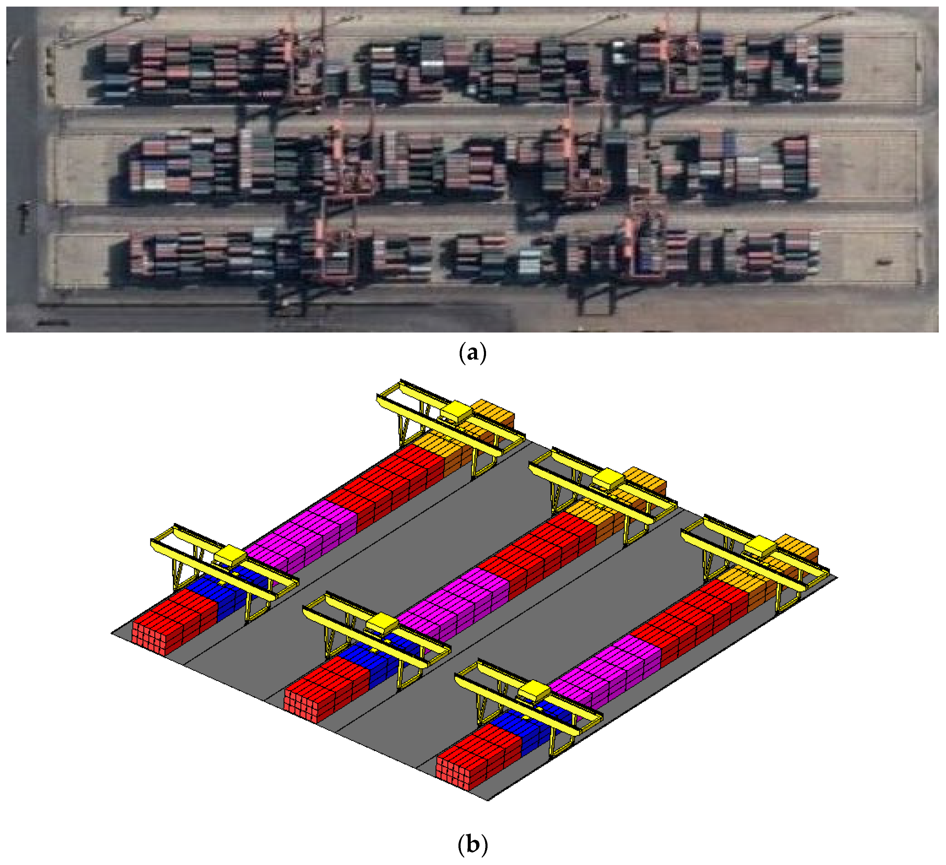
2.3. Environment Modelling

To be able to facilitate the study of the UAV path planning method, this paper establishes a 3D model based on the container yard environment in Figure 3. This model visually represents the container terminal yard environment, comprising key elements that could influence path planning outcomes, such as RMGCs, RMGCTs, and containers. The establishment of this 3D model lays the foundation for subsequent UAV path planning research.

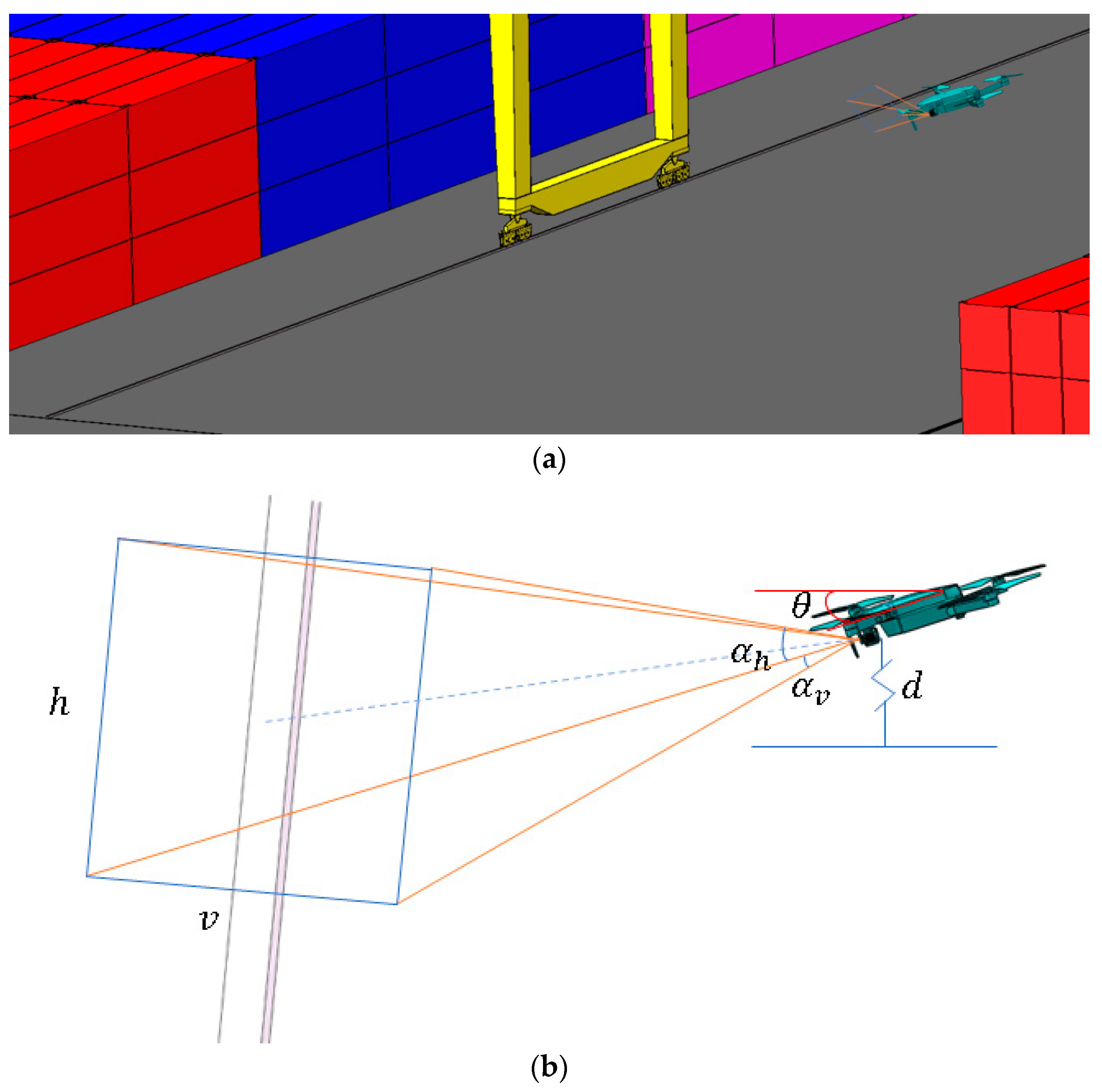
2.4. Viewpoint Selection

The collection of viewpoints necessitates a series of high-resolution visible-light camera settings. The high-resolution visible-light camera carried by the UAV only needs to capture the surface of the RMGCTs under examination (see Figure 4a). The choice of viewpoint is a very important step in the inspection process, and it is related to the final inspection’s efficiency and quality.

In this paper, a high-definition visible-light camera is utilized as the inspection device, and the field-of-view (FOV) constraints of the high-definition visible-light camera are modelled first. The FOV of a high-resolution visible-light camera is regarded as a rectangular grid. The angle $\theta$ represents the FOV of the camera lens. The size of the grid is related to the vertical viewing angle ${\alpha }_v$ and horizontal viewing angle ${\alpha }_h$ of the high-definition visible-light camera and the distance $d$, which is the vertical distance from the UAV to the orbital surface. In Figure 4b, the relationship between the various variables is shown. The equations that must be satisfied are

$$\mathrm{v}\approx 2\times \left(\frac{d}{\mathit{tan}\left|\theta \right|}-\frac{d}{\mathit{tan}\left(\left|\theta \right|+\frac{{\alpha }_v}{2}\right)}\right),$$

(1)

$$\mathrm{h}\approx 2\times \left(\frac{d}{\mathit{tan}\left|\theta \right|}-\frac{d}{\mathit{tan}\left(\left|\theta \right|+\frac{{\alpha }_h}{2}\right)}\right),$$

(2)

where v and h are the horizontal and vertical dimensions of the field-of-view grid, respectively.

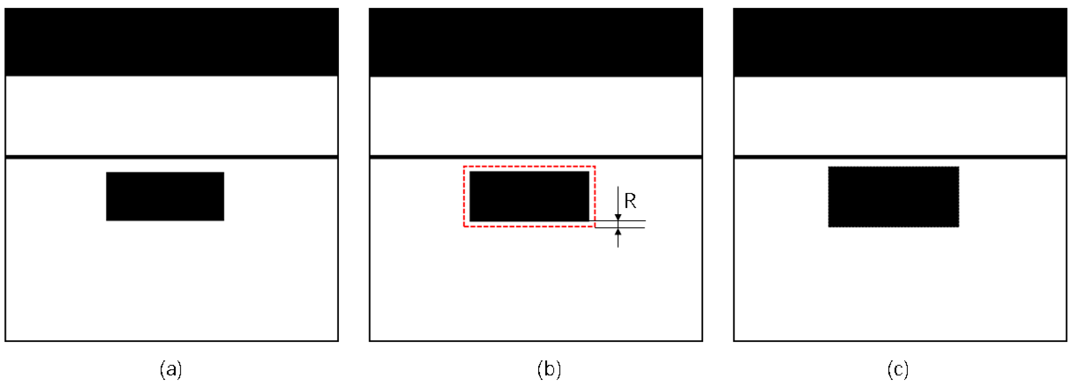
UAVs are subject to various interferences during flight, such as wind disturbance, positioning errors, and other anomalies. Therefore, it is very necessary to compensate for errors generated during the flight of the UAV. The direction of the error is mainly horizontal and vertical. As shown in Figure 5, the black area is the ideal FOV for a high-resolution visible-light camera. The yellow area in the FOV is under the error of the high-resolution visible-light camera. The blue area is the FOV of the high-resolution visible-light camera after error correction. H and V represent the maximum errors in the vertical and horizontal directions, respectively. Therefore, the position change range of the UAV in the vertical direction $h^{*}$ is

$$\mathrm{h}-\mathrm{H}\le h^{*}\le \mathrm{h}+\mathrm{H},$$

(3)

and the range of positional change in the horizontal direction $v^{*}$ is

$$\mathrm{v}-\mathrm{V}\le v^{*}\le \mathrm{v}+\mathrm{V}.$$

(4)

Then take the minimum $h^{\mathrm{*}}$ and $v^{\mathrm{*}}$ that satisfy the above inequalities (3) and (4), substituted into the following formulas:

$$d_{\mathit{min}H}=\frac{h^{\mathrm{*}}\times \mathit{tan}\left|\theta \right|\times \mathit{tan}(\left|\theta \right|+\frac{{\alpha }_h}{2})}{2\left(\mathit{tan}\left(\left|\theta \right|+\frac{{\alpha }_h}{2}\right)-\mathit{tan}\left|\theta \right|\right)},$$

(5)

$$d_{\mathit{min}V}=\frac{v^{\mathrm{*}}\times \mathit{tan}\left|\theta \right|\times \mathit{tan}(\left|\theta \right|+\frac{{\alpha }_v}{2})}{2\left(\mathit{tan}\left(\left|\theta \right|+\frac{{\alpha }_v}{2}\right)-\mathit{tan}\left|\theta \right|\right)}.$$

(6)

The shortest distance based on height $d_{\mathit{min}H}$ and the shortest distance based on breadth $d_{\mathit{min}V}$ from the high-resolution visible-light camera to the RMGCTs can be obtained.

Therefore, the shortest distance $d_{min}$ from the high-resolution visible-light camera to the RMGCTs is

$$d_{min}=\max (d_{\mathit{min}V},d_{\mathit{min}H}).$$

(7)

2.5. Precise Positioning of the UAV

The positioning problem of the UAV is very important in the process of UAV inspection, and it is related to whether the UAV can effectively execute the planned flight plan. When the UAV performs its task in an open outdoor scene, the GPS positioning system can meet the positioning requirements of the UAV due to the relatively high signal strength of the GPS. However, when the UAV flies to a location where the GPS signal is blocked, the GPS positioning system becomes ineffective.

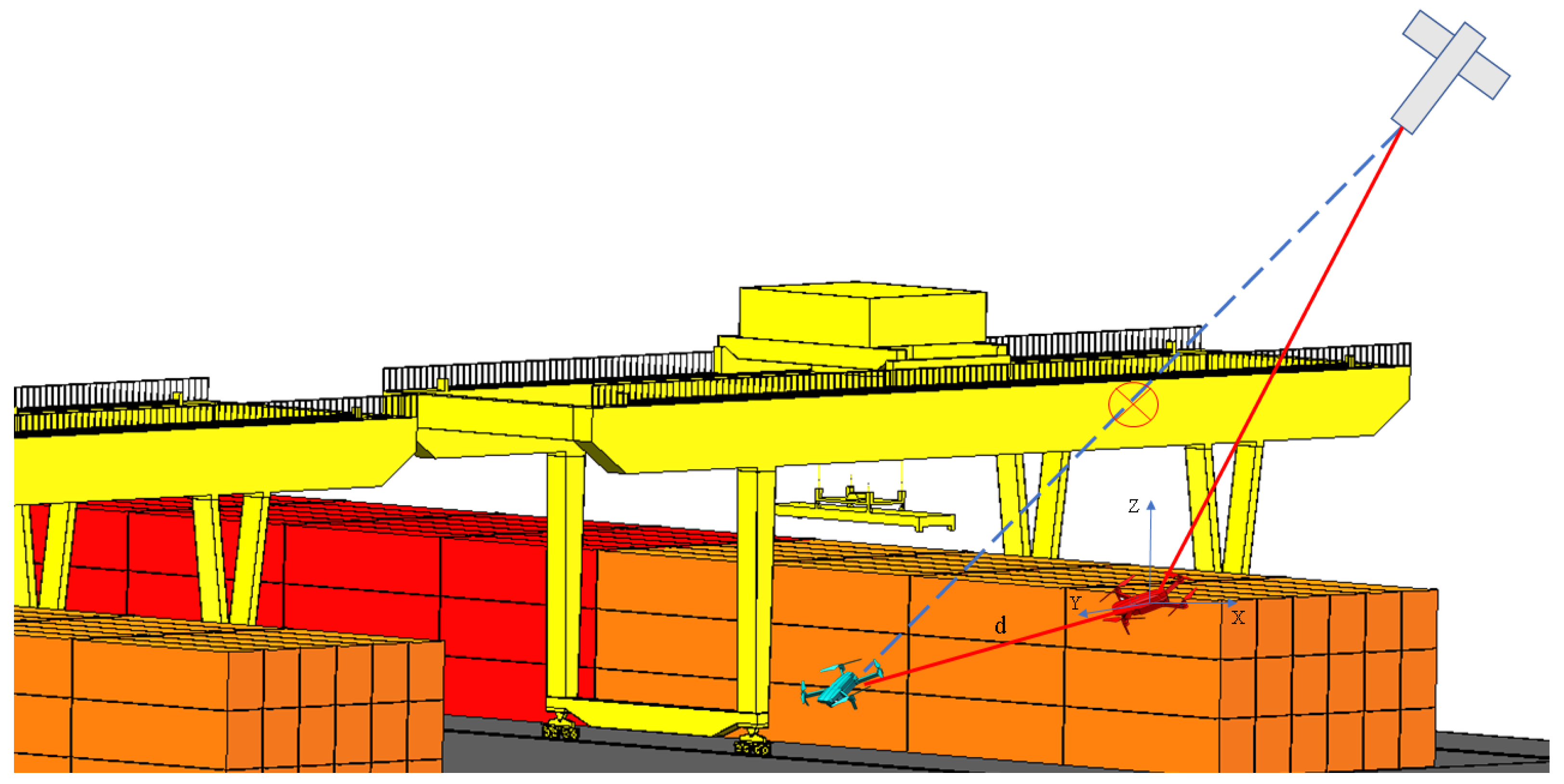
In this paper, it is necessary to consider the positioning of the UAV when it flies under the main beam of the gantry crane or when there is an obstructed part of the container. To ensure the UAV reaches its precise location, this paper employs the UAV cooperative positioning method to locate the GPS signal when it is blocked. As shown in Figure 6, the red UAV is a co-positioning UAV, which can receive signals from satellites at the same time as the inspection UAV. It needs to carry a vision sensor to achieve precise positioning of the inspection UAV in the case of a weak GPS signal. Here, d represents the distance between the two UAVs, while μ and τ denote the pitch and azimuth angles of the inspection UAV relative to the co-location UAV. They must satisfy the following conditions:

$$\mathsf{\Delta }\mathrm{z}=d\times \sin \mu ,$$

(8)

$$∆x=d\times \cos \mu \cos \tau ,$$

(9)

$$∆y=d\times \cos \mu \sin \tau .$$

(10)

Utilizing the aforementioned method, even if the main positioning UAV cannot directly obtain accurate positioning due to the weak GPS signal, the co-positioning UAV can indirectly obtain the precise positioning of the main positioning UAV.

2.6. Obstacle Avoidance

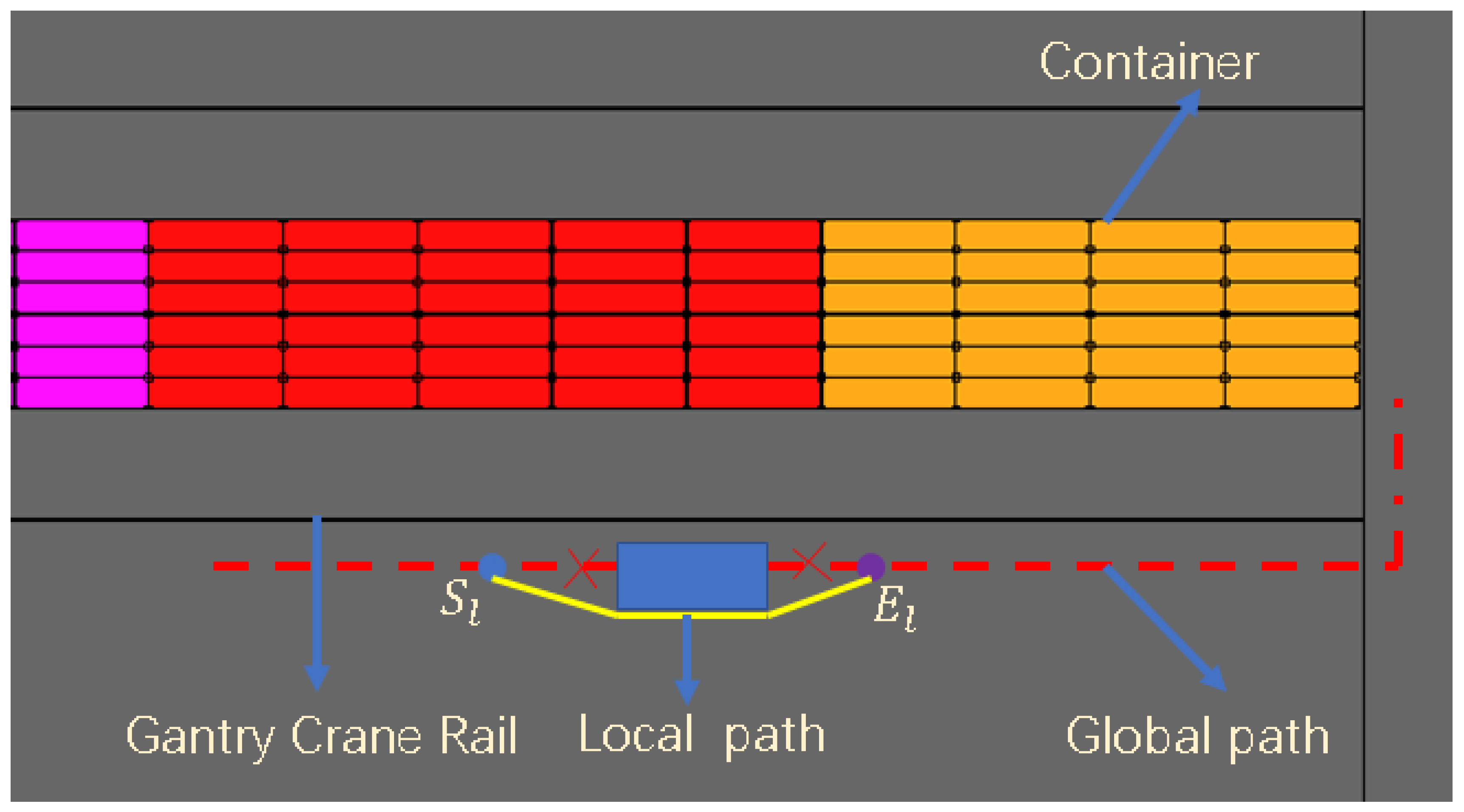
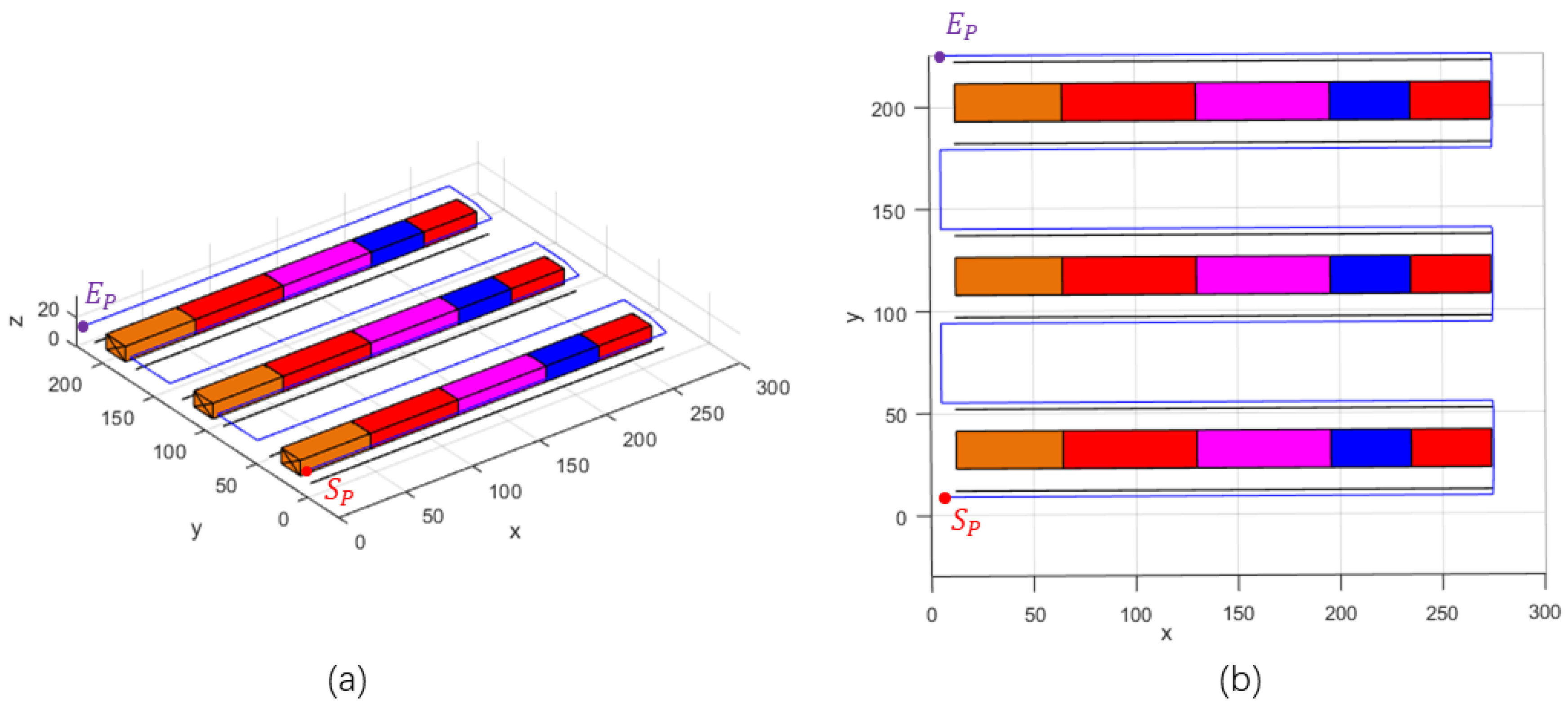
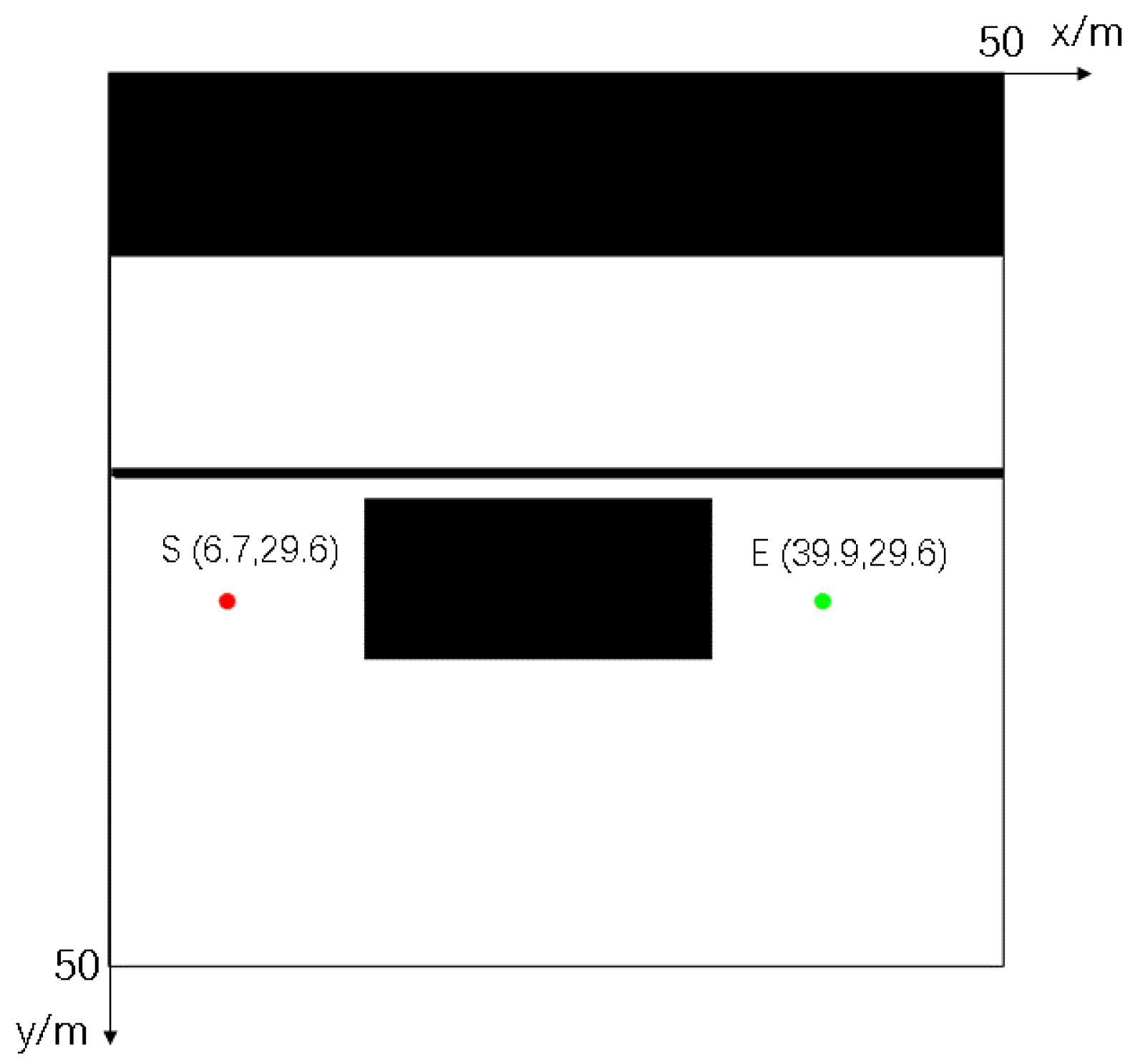
When the UAV is performing an inspection task, it will encounter many local conditions, such as a small car, other UAVs in flight, pedestrians, etc. The appearance of these unpredictable obstacles will affect the flight of the UAV so that the UAV can no longer fly along the planned global path, thus necessitating local path planning. An unexpected scenario is assumed in this paper, as shown in Figure 7. This scenario assumes that the UAV encounters a moving car during flight, which then needs to force the UAV to change its previous planned trajectory. This paper uses the IB-RRT* algorithm for localized path planning. In Figure 7, the blue box represents the stationary car, the red dashed line represents the global path, and $S_l$ and $E_l$ represent the start and end points of the local path, respectively, both of which intersect with the global path. The yellow paths represent the local paths planned using the IB-RRT* algorithm. Avoiding real-time static obstacles using the IB-RRT* algorithm allows the UAV to eventually continue the flight of the global path.

2.7. Geometric Optimization of the Path

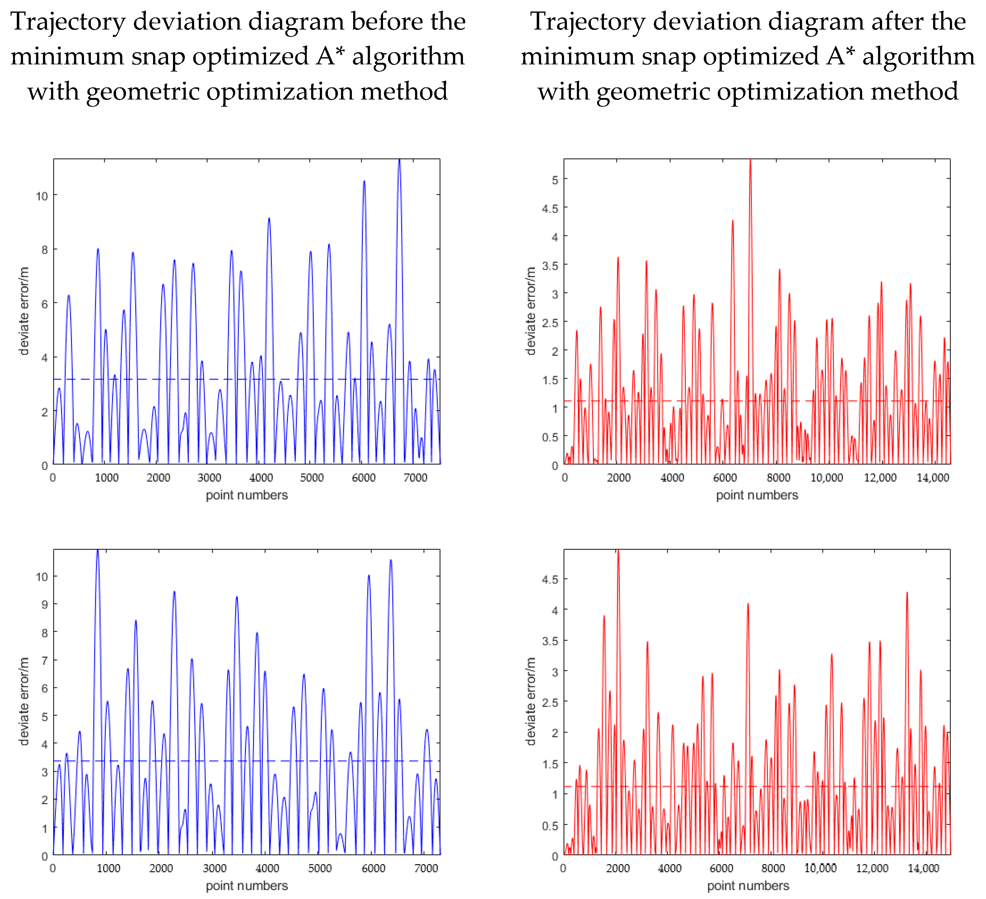
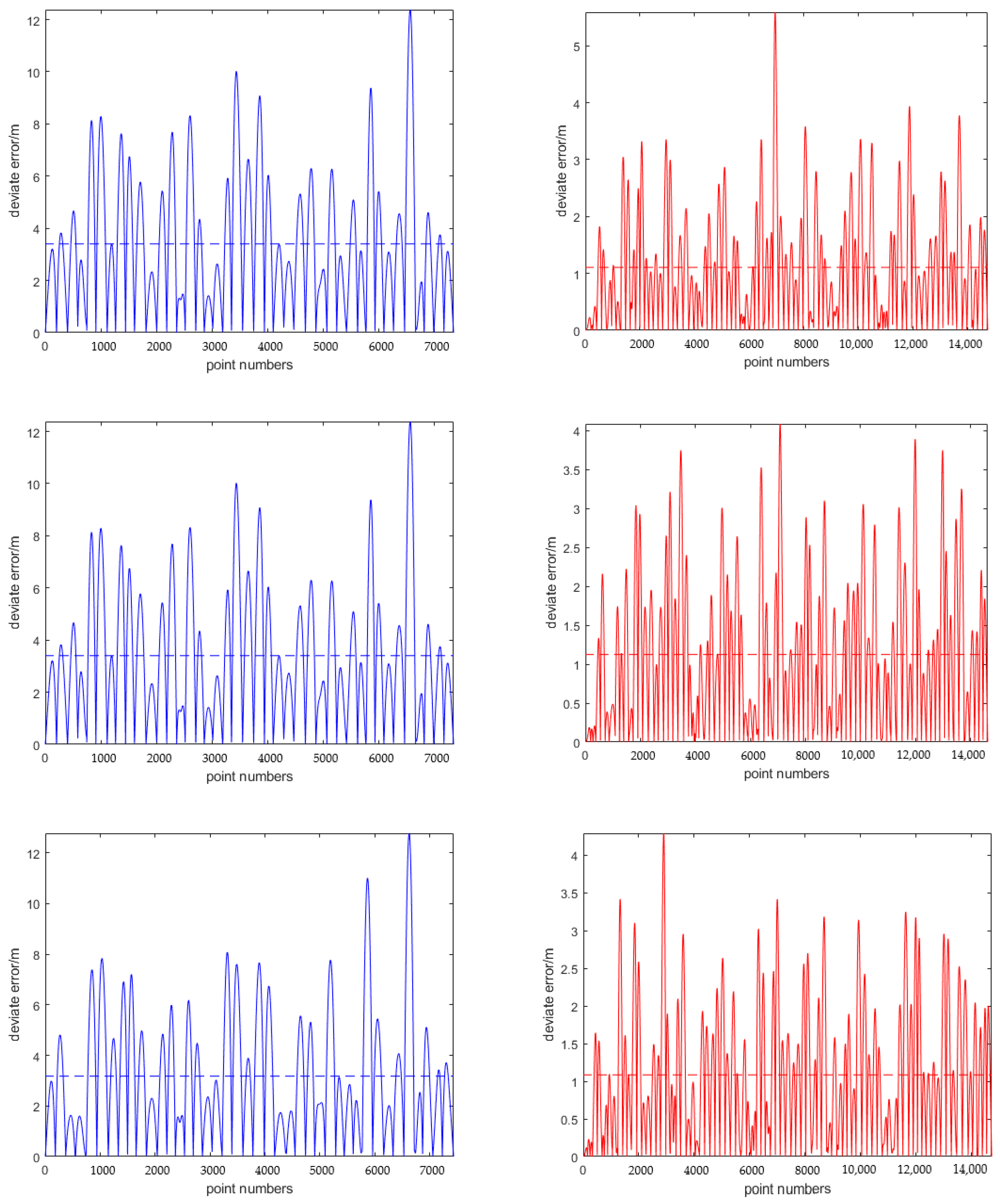
The A* algorithm does not consider the velocity and acceleration constraints of the UAV when planning the route, resulting in paths that are prone to abrupt changes. As the angle of the two-line direction vectors gets larger, the path cannot meet the flight requirements of the UAV. In trajectory planning, the deviation of the generated trajectory from the planned path will be bigger. Conversely, when the angle of the direction vector of the two lines is smaller, the path can meet the flight requirements of the UAV. In trajectory planning, the smoother the generated trajectory is, the smaller the deviation from the planned path. Two vectors with large angular variations can be equivalently replaced by a combination of multiple vectors with small directional variations. Utilizing this principle, this paper geometrically optimizes the UAV’s path by transforming the intersection of two vectors with large angles into a combination of multiple vectors with small angles, so that the trajectory of the UAV is smooth and the deviation distance is small.

In this paper, the method of constructing an isosceles triangle was employed, converting the large angle of two lines into two small angles, as shown in Figure 8. The original path A-D-G is transformed into A-B-H-I-F-G by constructing the isosceles triangles $\Delta BDF$, $\Delta BCH$, and $\Delta EFI$, which means the direction of the UAV does not change very much at one time. The specific steps involved are as follows:

(1) Construct an isosceles triangle $\mathsf{\Delta }BDF$. Ensure that the hypotenuse BF of the triangle does not intersect with the yard model. The lengths of BD and DF are denoted as $l_{BD}$ and $l_{DF}$, respectively. The steering angle of the UAV before optimization is $\alpha$.

(2) On line segment BD and line segment DF, take points C and E, respectively. Connect point C and point E, and select point H and point I, respectively, on segment CE. Points H and I equally trisect the line segment CE. The lengths of line segments BC, CH, IE, and EF are denoted as $l_{BC}$, $l_{CH}$, $l_{IE}$, and $l_{EF}$, respectively. The above lengths and angles must satisfy the following equations:

$$l_{\mathrm{B}\mathrm{D}}=l_{\mathrm{D}\mathrm{F}},$$

(11)

$$l_{\mathrm{B}\mathrm{C}}=l_{\mathrm{C}\mathrm{H}}=l_{\mathrm{I}\mathrm{E}}=l_{\mathrm{E}\mathrm{F}},$$

(12)

$$l_{\mathrm{B}\mathrm{C}}=\frac{2\left(l_{\mathrm{B}\mathrm{D}}{-l}_{\mathrm{B}\mathrm{C}}\right)\sin (\alpha /2)}{3}.$$

(13)

(3) Connect point B to point H and point I to point F. The optimized path A-B-H-I-F-G can be obtained. The steering angle after geometric optimization of the UAV is $\beta$. Obviously, $\alpha$ and $\beta$ satisfy the following equation:

$$\beta =\frac{180°-\alpha }{4}.$$

(14)

Utilizing the aforementioned method, the inspection path length of the UAV is shortened. At the same time, the UAV’s individual steering angles are also reduced. This process is referred to as geometric optimization.

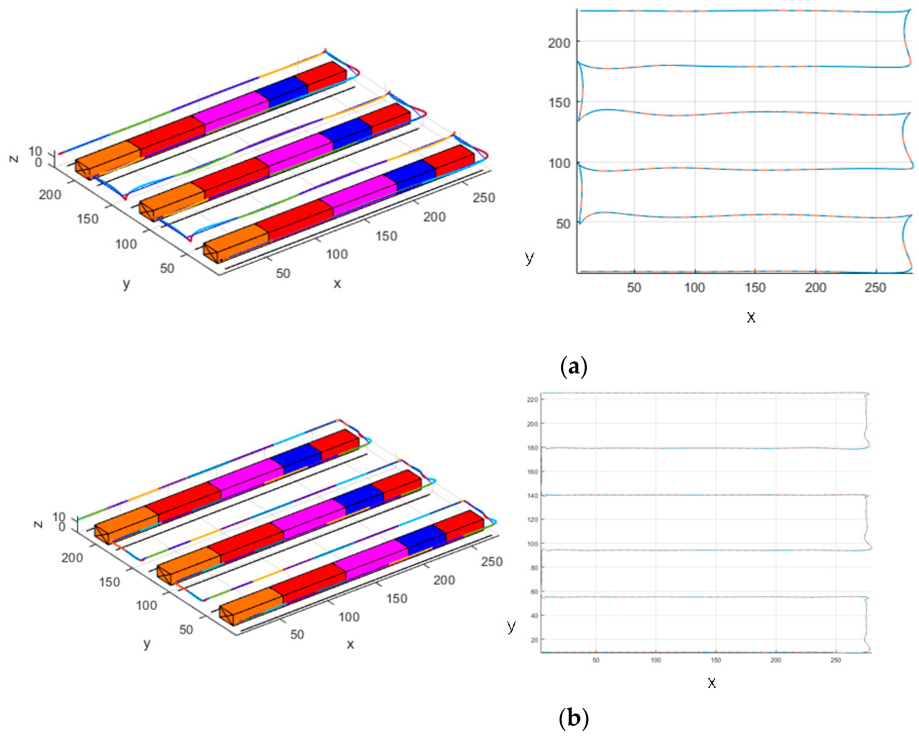
2.8. Trajectory Optimization

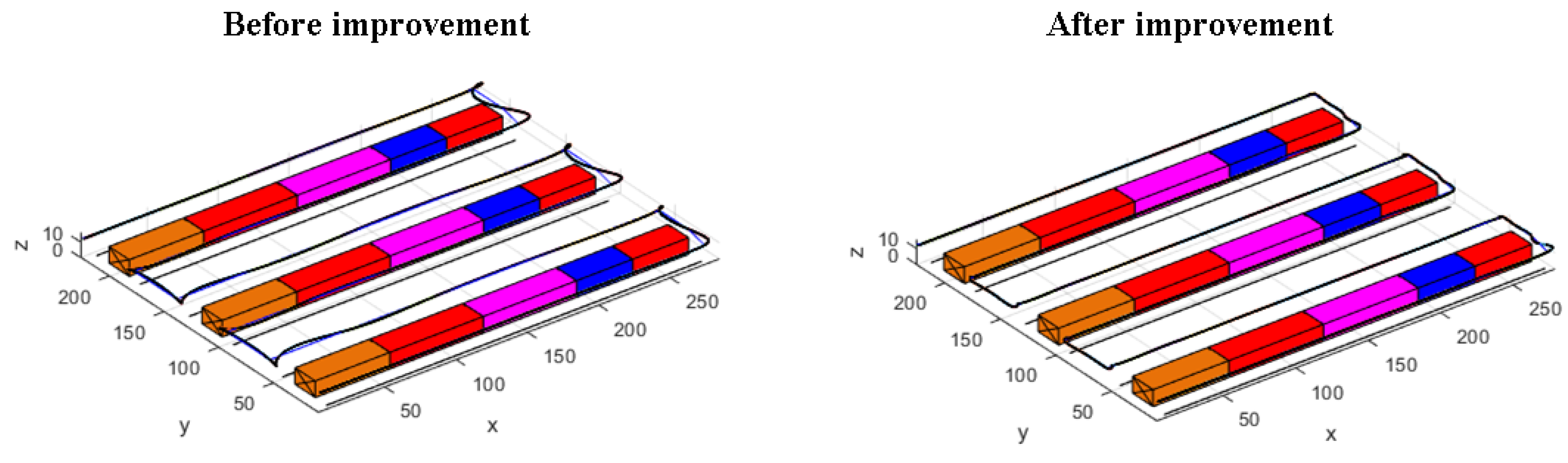
Following UAV path planning and geometric pre-processing of the path, a path for container terminal yard inspection is obtained in this paper. Next, UAV trajectory planning is conducted based on this path. The minimum snap method is adept at facilitating trajectory planning for UAVs with high degrees of freedom. This method can plan a series of sparse path points into a smooth curve or dense path points. However, the trajectory length of a UAV trajectory planned by the original minimum snap method is long and the deviation of the trajectory from the path is large. Therefore, UAV trajectory planning is carried out using the minimum snap method with the flight corridor constraint added, where the UAV trajectory can be restricted to a certain range to plan, which makes the UAV trajectory length shorter and the trajectory deviation smaller. Define $t_i$ as the unit vector extending from $r_i$ to $r_{(i+1)}$, where $r_i$ represents the coordinates of the i-th path point. The vertical distance vector $d_i\left(t\right)$ from line segment i is defined as follows:

$$d_i\left(t\right)=\left(r_T\left(t\right)-r_i\right)-\left(\right(r_T\left(t\right)-r_i)·t_i)t_i,$$

(15)

the width ${\delta }_i$ of the corridor under the infinite criterion is satisfied by [29],

$${\left|\right|d_i\left(t\right)\left|\right|}_{\mathrm{\infty }}\le {\delta }_i.$$

(16)

The UAV trajectory effect after adding the flight corridor constraint, which makes the UAV trajectory shorter and the trajectory deviation smaller, improves UAV inspection efficiency and saves energy.

3. Description of Methods

To improve the inspection efficiency of RGMCTs, a high-resolution visible-light-camera-equipped UAV path planning method is proposed in this paper.

3.1. Conditional Constraints of the UAV

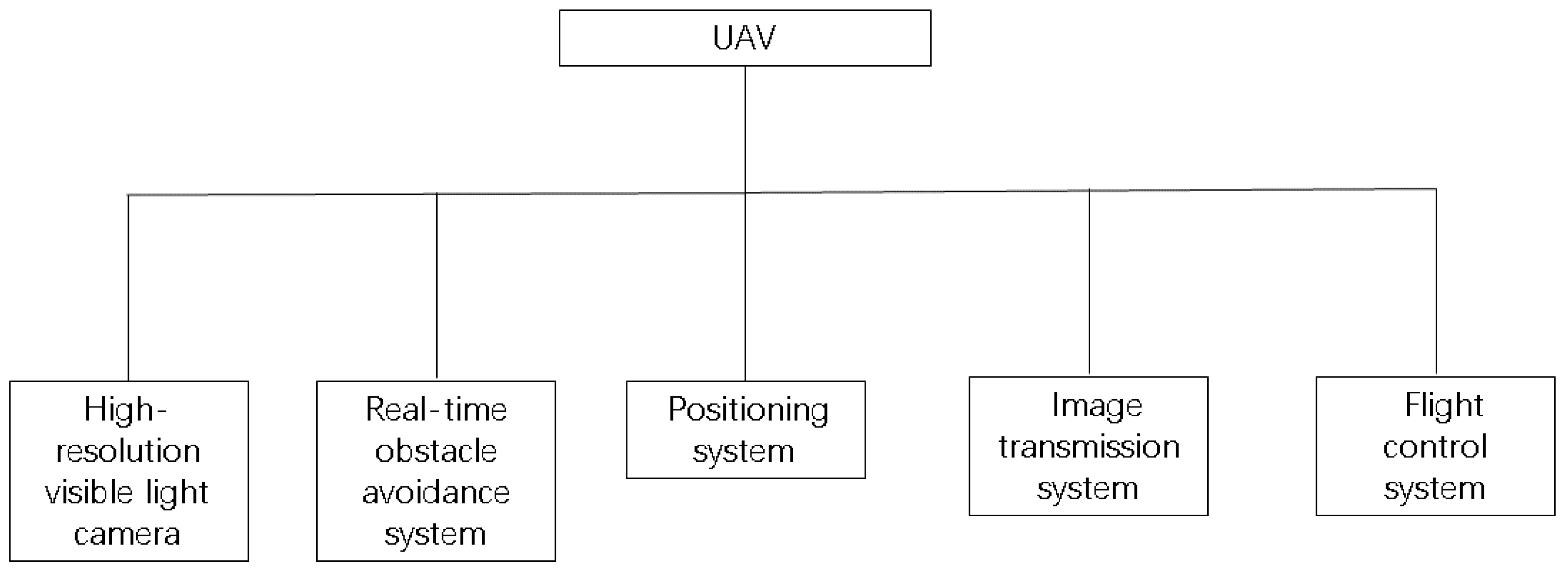
(1) Equipment that should be carried on the UAV: The equipment that the UAV should carry is shown in Figure 9. The UAV should be equipped with a high-resolution visible-light camera for image collection, a real-time obstacle avoidance system for avoiding real-time obstacles, a positioning system for UAV positioning, an image transmission system for image transmission, and a flight control system for aircraft flight.

(2) Requirements of the high-resolution visible-light camera: The high-resolution visible-light camera position used in this article is the solution of most commercial UAVs on the market, which install the high-resolution visible-light camera under the UAV. As shown in Figure 10, this is exemplified by the DJI series of UAV, equipped with a high-resolution visible-light camera. The position of the camera on the UAV should be able to capture the inspection surface, and the high-resolution visible-light camera can rotate at a certain angle to adapt to different situations.

(3) Requirements of the real-time obstacle avoidance system: This system mainly senses real-time obstacles, performs real-time path planning, and transmits the planned path to the flight control system. The system should include a 2D lidar sensor and a local path planning module. When the 2D lidar sensor inspects an unpredictable obstacle, the local path planning module can avoid the real-time obstacle with local path planning and finally return to the planned global path.

(4) Requirements of the positioning system: This system is mainly used for positioning during the flight of the UAV to obtain the real-time position. In this paper, the UAV is equipped with a GPS and a SLAM system for synchronous modeling and positioning of the UAV. The SLAM system uses the 2D lidar sensor described in (3) for real-time synchronous modeling and positioning.

(5) Requirements of the image transmission system: This system mainly sends the collected image information to the ground station system.

(6) Requirements of the ground station system: This system is mainly used for the global path planning of the UAV, and conveys the planned path information to the flight control system of the UAV. In addition, the ground station system is also used to receive the image information sent back by the UAV.

(7) Requirements of the flight control system: This system of the UAV mainly receives the planned path information to control the UAV so that the UAV can fly along the planned path. In the process of control, the speed and acceleration constraints of the UAV must be taken into consideration to minimize the deviation of the final flight trajectory from the planned path.

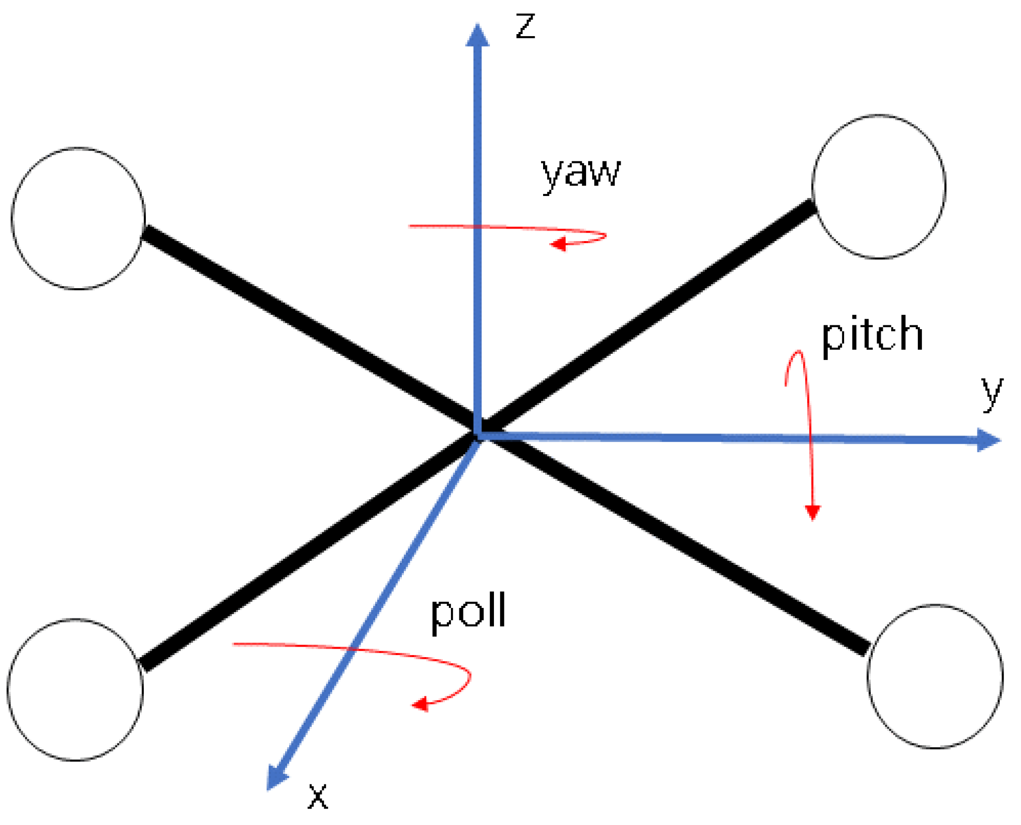
(8) The airframe requirements of the UAV: The UAV’s structure must accommodate six degrees of freedom, as shown in Figure 11. They are the displacement degrees of freedom in the three directions of x, y, and z and rotational degrees of freedom around the three axes, that is, yaw, roll, and pitch. To ensure the safety of flying in the yard, the airframe material of the UAV should be constructed from anti-static materials. The size of the airframe should be minimized to ensure the safety of the UAV during flight. But the size should not be too small; it must be balanced with load and power.

(9) The distance from the high-resolution visible-light camera to the RMGCTs: In the choice of distance, the primary consideration is ensuring the clarity of the captured image. Secondly, it is vital to compensate for any errors. The horizontal and vertical errors in the camera’s FOV are compensated by changing the distance between the high-resolution camera and the shooting surface by the method described in Section 2.4.

The aforementioned nine points serve as constraints for the UAV, which are very necessary in this paper.

3.2. Experimental Environment Setup

In this paper, the 3D model of a container terminal yard is converted into a simulation model for UAV path planning. During the conversion process, a conversion ratio of 100:1 was selected. The unit of measurement for the converted model is meters. For some detailed parts of the container terminal yard, appropriate simplifications are made without affecting the inspection. For example, RMGCs in the environment do not affect the results of UAV path planning; these gantry cranes can be omitted for environmental parsimony. The converted simulation model is shown in the red graph in Figure 12.

3.3. Global Path Planning

In this paper, a UAV path planning method based on container terminal yard inspection is proposed. In the container terminal yard environment, this paper combines local path planning and global path planning. The strategy of this paper is to plan a superior global UAV path and also to plan a shorter path in a shorter time when the UAV encounters static real-time obstacles.

The framework of this paper is shown in Figure 13. First, the model of the container terminal yard is established. Second, the UAV’s inspection viewpoint is determined. The location of the viewpoint mainly aligns with the normal direction of the inspection surface. Next, the shortest path through all viewpoints is planned with the A* algorithm. Fourth, a UAV trajectory is planned by an improved minimum snap method. Fifth, when the UAV encounters a real-time static obstacle, a path is planned in a shorter time by the IB-RRT* algorithm to avoid the real-time obstacle and return to the global trajectory.

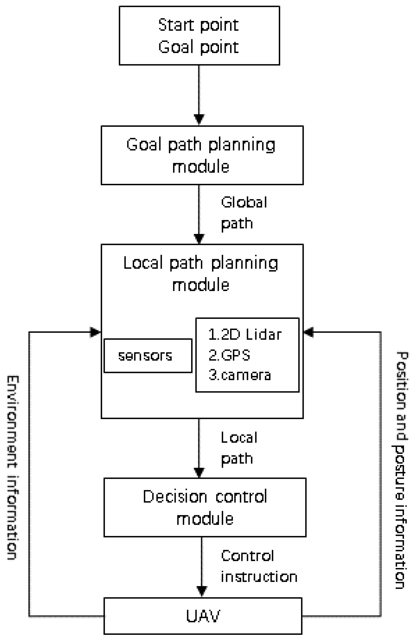
3.4. Local Path Planning

During the flight, the UAV may encounter unforeseen obstacles, such as a port trolley, that were not present in the original scene. In the face of an emergency, the UAV must make changes to the original path in response to the emergent quasi-conditions to perform local path planning. During the local path planning process, the UAV needs to avoid real-time obstacles and finally return to the predefined path. Sensors are critical at this stage. UAVs need to obtain obstacle information through sensors to acquire their relative position changes and explore unknown environments so that they can perform simultaneous localization and mapping (SLAM) at the same time and find a local path [30,31].

In Figure 14, the block diagram for UAV planning and control is shown. It can be seen from Figure 14 that local path planning plays an important role in the entire framework.

4. Simulation

4.1. Global Path Planning

4.1.1. Simulation Experiment Result

The simulation experiment was conducted on a computer with an Intel(R) Core (TM) i7-3540M CPU @3.00GHz. The simulation experiment environment was the simulation environment established in Figure 12. After UAV path planning, the global path for UAV inspection obtained in this paper is shown in Figure 15.

The blue line in Figure 15 was the planned global path using the A* algorithm. The length of the path was 1834.897 m. This was a path planned without considering the kinematic and dynamical constraints of the UAV, and the path was a fold at the turn, so it could not be directly used for the flight of the UAV.

Next, trajectory planning for the UAV was carried out; i.e., a smooth trajectory was generated along the global path using the minimum snap method, which is shown in Figure 16a. From Figure 16a, it can be seen that the UAV trajectory had a large deviation at and near the turn (the trajectory deviation was the error distance between the generated UAV trajectory and the path). Figure 16b shows the global path optimized using the minimum snap algorithm after geometric optimization. This trajectory was significantly improved at the corner compared to the original trajectory.

4.1.2. Simulation Results Analysis

The above experimental results show the schematic diagram of the trajectory effect before and after trajectory optimization. From Figure 16, it can be seen that the optimized UAV had a large improvement in trajectory deviation. To prove the validity of the conclusion, five simulation experiments were conducted for the trajectory planning method before the improvement and the trajectory planning method after the improvement, and the trajectory length and trajectory deviation before and after the improvement was compared.

Table 1. Comparison of UAV trajectory length before and after the minimum snap optimized A* algorithm with geometric optimization.

Experimental Serial Number	Length of Trajectory before Improvement (m)	Length of Trajectory after Improvement (m)	Optimized Trajectory Length (m)	Improvement Percentage
1	1917.223	1873.703	43.520	2.27%
2	1946.701	1870.354	76.347	3.92%
3	1917.223	1874.921	42.302	2.21%
4	1937.157	1874.120	67.037	3.25%
5	1919.038	1869.729	49.309	2.57%
Average	1927.468	1872.565	54.903	2.85%

shows the trajectory lengths for the UAV before and after the improved method and the percentage improvements. From Table 1, it can be seen that the average trajectory length planned by the improved method before the five experiments was 1927.468 m, the average trajectory length planned by the improved method was 1872.565 m, the average improved trajectory length was 54.903 m, and the average improvement ratio for the trajectory length was 2.85%. Within five experiments, the maximum improvement length for the UAV trajectory planned by the improved method was 76.347 m compared with the pre-improved method, and the maximum improvement ratio was 3.92%.

Therefore, the improved method using the minimum snap algorithm with the addition of geometric optimization had a shorter UAV trajectory compared with the planned UAV trajectory before the improved method, and the improved UAV trajectory could improve inspection efficiency and save the energy of the UAV.

Trajectory deviation is an important indicator to evaluate the trajectory of a UAV. The smaller the trajectory deviation, the more the trajectory can meet UAV inspection requirements. Figure 17 shows the trajectory deviation graphs of five simulation experiments before and after the improved method. From Figure 17, it can be seen that the trajectory deviation of the UAV after the improvement method was improved compared with the trajectory deviation before the improvement method.

Table 2. Comparison of UAV trajectory length before and after the minimum snap optimized A* algorithm with geometric optimization.

Experimental Serial Number	Average Deviation before Improvement (m)	Average Deviation after Improvement (m)	Optimized Average Deviation (m)	Improvement Percentage
1	3.162	1.114	2.048	64.7%
2	3.363	1.114	2.249	66.9%
3	3.162	1.106	2.056	65.0%
4	3.403	1.124	2.279	67.0%
5	3.175	1.086	2.089	65.8%
Average	3.253	1.109	2.144	65.9%

presents the average deviations before and after improvement, optimized average deviations, and the UAV trajectory deviation percentages for the five experiments employing the minimum snap optimized A* algorithm with geometric optimization. According to Table 2, the maximum average improvement deviation distance was 2.279 m and the improvement percentage was 67.0%. In the five UAV trajectory planning experiments, the average trajectory deviation distance before the improvement was 3.253 m, the average trajectory deviation distance after the improvement was 1.109 m, the average improvement deviation was 2.144 m, and the average improvement percentage was 65.9%.

Therefore, it can be seen that the UAV trajectory deviation generated using the minimum snap algorithm with the addition of geometric optimization was greatly improved in terms of trajectory deviation. Thus, the trajectory deviation of the UAV trajectory was small.

4.1.3. Trajectory Tracking

Through the above experimental results and analysis, it can be seen that the UAV trajectory adding geometric optimization and corridor constraints was improved in terms of trajectory length and trajectory deviation. The trajectory tracking effect was another important criterion to evaluate the planned UAV trajectory, and this paper judged whether the planned UAV trajectory was reasonable by the deviation of the tracking.

After tracking the trajectory, one of the groups of UAV trajectory tracking effects obtained in this paper is shown in Figure 18, where the coloured lines are the planned UAV trajectory and the black lines are the trajectory traced by the UAV. From Figure 18, it can be seen that the black lines almost cover the coloured lines, which meant that the trajectory was better after optimizing the UAV path using the minimum snap algorithm with the addition of geometric optimization.

Figure 19 shows the deviations of trajectory tracking before and after the improved method. The trajectory deviation was mainly the x, y, z position error and yaw angle error. The position error and yaw angle error of x, y, z before the improvement were up to 0.05 m, 0.06 m, ${7\times 10}^{-3}$ m, and ${{8\times 10}^{-6}}^{°}$, and the position error and yaw angle error of x, y, z after the improvement were up to 0.02 m, 0.02 m, ${2.5\times 10}^{-3}$ m, and ${{2.5\times 10}^{-7}}^{°}$. Therefore, the UAV trajectory error after the improvement was much smaller than before the improvement. The tracking error was much smaller than before the improvement, and it met the flight requirements of UAVs.

4.2. Local Path Planning

When the UAV flies along the planned global trajectory, it will encounter some local obstacles. At this time, the UAV needs to change the global flight trajectory and perform local path planning. The purpose of this part of the experiment is to plan a short local path in a short time to avoid local obstacles. The environment selected for this local experiment is the one in Figure 7, assuming that the UAV in flight encounters a parked car.

The scene was transformed into a binarized map, as shown in Figure 20a. Next, the local obstacles were enlarged; i.e., the outline of the cart was extended outward to the safe flight distance R of the UAV, as shown in Figure 20b. The final obtained binarized map after the extended map is shown in Figure 20c, so that the map of local path planning was established.

The coordinate system shown in Figure 21 was established for this map, the coordinates of the starting point were (6.7,29.6), the coordinates of the ending point were (39.9,29.6), and the paths between the two points were planned using the RRT, RRT*, BI-RRT*, and IB-RRT* algorithms, respectively, where the number of iterations of the RRT*, BI-RRT*, and IB-RRT* algorithms was set to 700. The planning effects of the paths and the data are shown in Figure 22.

From Figure 22, it can be seen that the IB-RRT* algorithm plans shorter paths and took less time to plan the paths compared with the RRT, RRT*, and BI-RRT* algorithms, which is very beneficial for local path planning for UAVs. To prove the accuracy of the experimental results, 10 experiments were conducted using each of the four algorithms in the experimental environment to obtain their path planning times and the lengths of the paths.

Table 3. Path length and time planned by the RRT, RRT*, BI-RRT*, and IB-RRT* algorithms in ten experiments.

Algorithm Name	Average Processing Time (s)	Average Time Improvement Percentage	Average Path Length (m)	Average Path-Length Improvement Percentage
RRT	${2.352}_{-0.572}^{+0.595}$	-	${45.155}_{-7.166}^{+7.353}$	-
RRT*	${5.218}_{-1.839}^{+0.979}$	−121.85%	${35.619}_{-0.744}^{+1.125}$	21.12%
BI-RRT*	${2.421}_{-0.127}^{+0.115}$	−2.93%	${35.355}_{-0.350}^{+0.451}$	21.70%
IB-RRT*	${1.080}_{-0.071}^{+0.158}$	54.08%	${35.286}_{-0.303}^{+0.434}$	21.86%

shows the average values of path planning time and path length for the four algorithms across ten experiments. These results were obtained under the same computational conditions. Additionally, the table includes the percentage improvements for the RRT*, BI-RRT*, and IB-RRT* algorithms compared with the RRT algorithm. The table shows that the paths planned by the RRT* and BI-RRT* algorithms were shorter and straighter in path length than the paths planned by the RRT algorithm, but that the path planning time was longer. the IB-RRT* algorithm had a relatively shorter path planning time and path length compared with the RRT, RRT*, and BI-RRT* algorithms. Its average time for path planning in ten experiments was 1.080 s, which is a 54.08% improvement over the time required for path planning by the RRT algorithm. The average path length planned in ten experiments was 35.286 m, which is a 21.86% improvement over the path length planned by the RRT algorithm. This shows that the IB-RRT* algorithm was superior to the RRT, RRT*, and BI-RRT* algorithms in terms of planned path time and path length.

5. Conclusions

In this paper, a UAV trajectory planning framework for RMGCT inspection on a container terminal yard in a port environment has been proposed. The framework consists of two main parts. (1) The first is establishing an automated container yard experimental environment, selecting viewpoints, and performing a global UAV trajectory planning framework. This paper uses the A* algorithm for global path planning and the improved minimum snap algorithm for global trajectory planning. The final simulated experimental results show that the UAV trajectory length and trajectory deviation planned by the improved minimum snap algorithm improved by 2.85% and 65.9%, respectively, compared with those before the improvement, and that the trajectory tracking effect was good. (2) Local path planning for the UAV is carried out to avoid real-time static obstacles during UAV flight and continue the global flight. In this process, the sampling-based IB-RRT* algorithm was selected for local path planning in this paper, and the path length and path time planned by this algorithm were compared with the RRT, RRT*, and BI-RRT* algorithms for their planned path times and path lengths. The final simulated experimental results indicate that the IB-RRT*, in ten simulation experiments, showed improvements of 54.08% in planning time and 21.86% in average path length compared with the RRT algorithm. This shows that the UAV trajectory planning framework has definite superiority. However, the framework in this paper also has some shortcomings, such as it not considering trajectory planning for UAVs in a dynamic environment; that the experiment was only carried out in a computer simulation environment; and that the actual algorithm running speed of the UAV was not taken into account. Furthermore, in this paper, optimizations of the global path algorithm and the local path algorithm were compared, and the ones with better performance were selected. The overall algorithm has not been compared with other algorithms that can be applied to the scenario. In the future, we will have to conduct more in-depth research in this area.